Adaptive Dynamic Thresholding Method for Fault Detection in Diesel Engine Lubrication Systems

Abstract

Fault detection in marine diesel engine lubrication systems is crucial for ensuring the long-term stable operation of diesel engines and the safety of maritime navigation. Traditional fixed-parameter alarm threshold methods lack flexibility and are prone to missing faults. Data-driven approaches like machine learning require high-quality data for fault samples. This study leverages the relative advantages of data mining methods and threshold techniques, proposing an adaptive threshold construction method based on dynamic parameter relationship inference. Employing an algorithm for inferring dynamic relationships among multiple parameters of the lubrication system builds an adaptive threshold detection model. Extensive diesel engine tests and actual fault data demonstrate that the proposed method can address the issues of missed faults encountered by static threshold methods and the low detection accuracy of machine learning approaches without the need for fault samples. This significantly enhances fault detection accuracy in marine diesel engine lubrication systems, offering considerable industrial practical value.

1. Introduction

The trend toward intelligent shipping has become a focal point in global maritime development, driving significant and rapid reforms toward digitization and intelligence in the maritime industry. As typical reciprocating power machinery, marine diesel engines exhibit complexity and diversity in faults due to the interactions among various systems. These complexities and the intricate causal relationships of faults increase the difficulty of predicting and diagnosing diesel engine malfunctions. The lubrication system of a diesel engine, which reduces wear and promotes cooling, is a critical component in ensuring its safe and stable performance. Therefore, diagnosing lubrication system failures and predicting related alarms play a crucial role in the reliable operation of diesel engines [1].

Currently, the prevalent monitoring method for marine diesel engine lubrication systems involves reading parameters from external pipelines and setting static alarm thresholds to detect and identify faults. This approach has issues with low accuracy, missed alerts, or false alarms, making it impossible to implement more comprehensive and accurate protection. In order to solve the limitation of fixed thresholds, some diesel engine experts have put forward an improved method based on threshold monitoring. Otero et al. [2] addressed the shortcomings and limitations of threshold alarms by proposing a solution for designing intelligent alarms. To overcome the limitations of traditional monitoring methods in nuclear power plants, Wu et al. [3] suggested the introduction of kernel principal component analysis (KPCA) in the online monitoring of nuclear power plant equipment. KPCA can provide more advanced fault warnings than existing threshold monitoring methods. In order to ensure the safe operation of major equipment, domestic and foreign diesel engine manufacturers and researchers have conducted a lot of research in the field of fault diagnosis. The fault diagnosis methods for marine diesel engine lubrication systems can be categorized into methods based on empirical knowledge, analytical models, and intelligent diagnostic methods driven by data [4].

Methods based on empirical knowledge are currently the most commonly used in engineering applications, typically relying on engineers’ professional knowledge and experience to judge and analyze faults. Streichfuss et al. [5] proposed a machine monitoring and maintenance management system based on expert systems. The diagnostic system is integrated with a maintenance planning and control system to provide data management free from contradictions and redundancies. Xu et al. [6] designed a belief rule-based (BRB) expert system for the fault diagnosis of marine diesel engines, which exhibits good accuracy and stability and can effectively identify concurrent faults. Unver et al. [7] conducted a systematic study of crankcase explosions in two-stroke marine diesel engines using the fault tree analysis method in a fuzzy environment for system reliability and shipping sustainability. However, methods based on empirical knowledge highly depend on human expertise, and their scientific validity and feasibility are subject to scrutiny.

Methods based on analytical models focus on the fault mechanism as the research subject. Krzysztofowicz R. et al. [8] proposed a Bayesian detection model designed for distributed sensor systems, where each sensor provides a detection probability to the central processor rather than an observation vector or detection decision. Moussa et al. [9] developed a physical model of the cooling and lubrication system of a marine diesel engine, which prepared an essential database for fault diagnosis and forecasting strategies for diesel engines. Although such methods can detect and diagnose faults, they are limited to scenarios where accurate physical or mathematical models can be established. The lubrication system of diesel engines provides lubrication for the moving parts of the whole machine and it has a complicated relationship with other systems. The accurate mathematical model of the operating fault is often difficult to obtain, which leads to the great limitations of the traditional model-based fault diagnosis method in application.

The large amount of diesel engine running process data acquisition provides good data conditions for the development of a data-driven intelligent diagnosis strategy. Intelligent diagnostic methods driven by data can, to some extent, overcome the shortcomings of the previous two approaches by reducing dependence on models and empirical knowledge. Using diesel engine running data and various data analysis methods, we can find the hidden information in the data. Further, the fault detection is carried out to realize the separation evaluation and decision of the lubrication system. Liu et al. [10] aimed at the coherent real-time monitoring of bearing status and proposed a gated recurrent unit-based fault monitoring structure to obtain a timely response to and preliminary classification of sudden faults. Ding et al. [11] considered the non-stationary stochastic characteristics of the current of PV strings and applied the local outlier factor (LOF) to detect faults in the PV system by evaluating the deviation between the observed data and the whole data. Zhao et al. [12] presented a novel intelligent fault diagnosis method based on an improved extreme learning machine (ELM). Alireza et al. [13] presented a condition monitoring and combustion fault detection technique for a 12-cylinder 588 KW trainset diesel engine based on vibration signature analysis using a fast Fourier transform, a discrete wavelet transform, and a multilayer perceptron (MLP). Liu et al. [14] proposed a fault diagnosis method based on fuzzy theory and a multidimensional model, indicating that a SVM (support vector machine) can handle the fuzzy information of fault samples and solve the indivisibility problem of SVM classification. Mariela et al. [15] used genetic algorithms and a classifier based on random forest (RF) to improve the gear fault detection’s reliability, effectiveness, and accuracy. Li et al. [16] described and evaluated the application by integrating empirical mode decomposition (EMD), kernel independent component analysis (KICA), Wigner bispectrum, and SVM for the fault diagnosis of marine diesel engines. Zhang et al. [17] analyzed aero-engine bearing vibration failure caused by low-pressure rotor imbalance and proposed a fault diagnosis model using the XGBoost algorithm. Wang et al. [18] established a hybrid fault monitoring scheme integrating manifold learning and the isolation forest (IF) to monitor the state of marine diesel engines. Cai et al. [19] proposed a novel fault detection and diagnostic method for diesel engines by combining rule-based algorithms and Bayesian networks (BNs) or back propagation neural networks (BPNNs). In addition, the influences of decomposed signal layers, sensor noise, and external excitation interference on fault diagnostic performance have been researched.

Although data-driven diagnostic methods can uncover information about the status of diesel lubrication systems, ample training data is a prerequisite for data-driven models to achieve high-precision diagnostic results. Moreover, in practical engineering applications, failures in diesel engine lubrication systems are low-probability events, and it is difficult to promptly detect and collect the data, resulting in a scarcity of fault samples [20]. As diesel engines operate under high-temperature, high-pressure, and high-velocity conditions over long periods, it is impossible to directly understand the diesel engine’s internal lubrication and cooling conditions through monitoring data, nor is it feasible to monitor fault trends [21]. How to use the existing oil pipeline monitoring data to monitor the internal dynamic change and fault trend of the lubrication system is the problem that needs to be solved in this paper.

In response to the problems identified with the above methods, this paper proposes a fault detection method for diesel engine lubrication systems based on adaptive dynamic thresholds. The main views and contributions are summarized as follows:

Dynamic parameter relationship inference algorithm: Utilizes the maximal information coefficient (MIC) [22] to evaluate the correlations among multiple parameters within the diesel engine lubrication system. This approach constructs relational surfaces and identifies critical parameters for more targeted analysis.

Adaptive dynamic threshold construction method: Develops adaptive thresholds for the diesel engine lubrication system under conditions devoid of fault samples. This enables a more precise detection of lubrication system faults, substantially reducing the likelihood of missed detections and false alarms.

Mechanistic study and analysis of lubrication system parameter relationships: Conducts a thorough investigation into the relationships between lubrication system parameters, culminating in proposing a mechanistic model. This model aims to deepen understanding of the system’s operation and enhance diagnostic accuracy.

The structure of this paper is as follows: Section 2 presents the theoretical framework for the dynamic parameter relationship inference algorithm and the adaptive dynamic threshold method for dynamic parameters; Section 3 introduces the experimental setup, data collection methods, and the experimental dataset; Section 4 discusses the experimental results; and the final section presents the conclusions.

2. Adaptive Threshold Fault Diagnosis Method

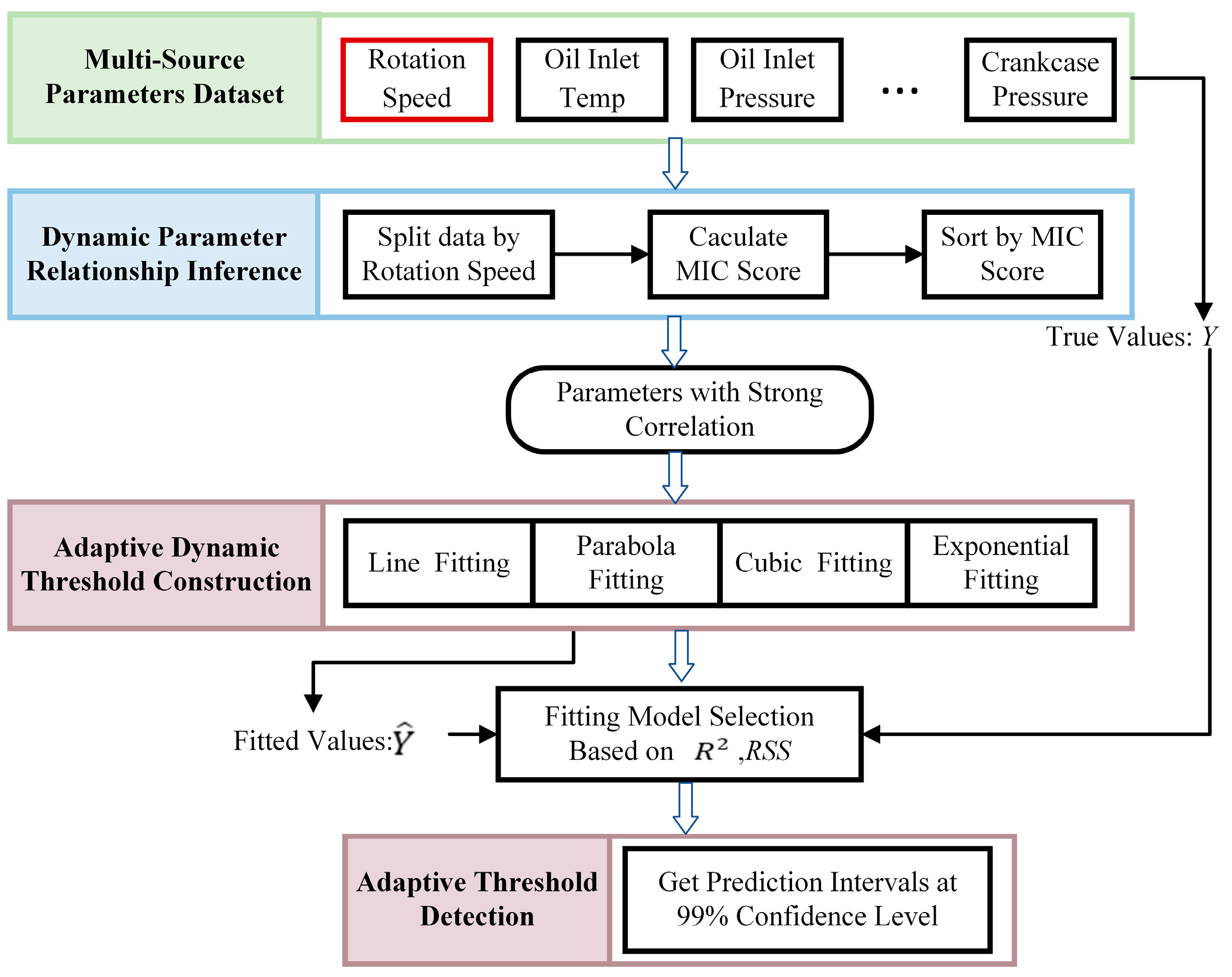
This paper introduces a fault detection algorithm for marine diesel engine lubrication systems, primarily comprising a dynamic parameter relationship inference algorithm and an adaptive dynamic threshold method for dynamic parameters. The dynamic parameter relationship inference algorithm delves into the intricate relationships between sensor data to identify potential patterns and correlations among different parameters under varying conditions. By employing advanced data analytics techniques, this algorithm can sift through large volumes of data to pinpoint critical parameters that significantly influence engine performance and reliability. Once these key parameters have been identified, the algorithm proceeds to construct adaptive thresholds that dynamically adjust in response to changes in engine speed and other relevant factors. This adaptability ensures that the thresholds remain pertinent and practical across a broad spectrum of operational conditions, thereby enhancing fault detection accuracy. The adaptive threshold detection algorithm is specifically designed to locate anomalies within predefined threshold ranges, focusing on trends that deviate from the norm. By analyzing data trends and variations, this algorithm can detect subtle shifts in engine behavior that may indicate the emergence of a fault or a deviation from expected performance levels. The entire algorithm model is shown in Figure 1.

Specifically, by utilizing a multi-source parameter dataset composed of data from different sensors in the diesel engine lubrication system, we determine the strongly correlated parameters under various operating conditions through mechanism analysis and MIC scoring. We then fit and model a large amount of data for these parameters to identify and establish a current “standard model” with a high degree of fit. The “standard model” under healthy conditions is used as a threshold condition for dynamic threshold fault diagnosis throughout the entire operational life cycle of the diesel engine. Naturally, as the operating time increases and machine performance deteriorates, the “standard model” will also undergo subtle changes.

2.1. Dynamic Parameter Relationship Inference Algorithm

The lubrication system encompasses a great deal of sensor information, typically including temperature signals from various locations, pressure signals, rotational speed signals, oil levels, etc., encompassing approximately 5–15 parameters to offer a comprehensive view of the lubrication system’s status. The challenge lies in extracting valuable information from the interrelations among these diverse parameters and how to synergistically utilize these sensor signals to enhance the utilization efficiency of this sensor information, which holds substantial latent value.

First, a matrix containing all sensor data from the lubrication system is constructed.

$$\mathrm{X}=\left[\begin{array}{c}{\mathrm{X}}^1\\ {\mathrm{X}}^2\\ ⋮\\ {\mathrm{X}}^{\mathrm{n}}\end{array}\right]=\left[\begin{array}{cccc}{\mathrm{x}}_1^1& {\mathrm{x}}_2^1& \dots & {\mathrm{x}}_{\mathrm{l}}^1\\ {\mathrm{x}}_1^2& {\mathrm{x}}_2^2& \dots & {\mathrm{x}}_{\mathrm{l}}^2\\ ⋮& ⋮& & ⋮\\ {\mathrm{x}}_1^{\mathrm{n}}& {\mathrm{x}}_2^{\mathrm{n}}& \dots & {\mathrm{x}}_{\mathrm{l}}^{\mathrm{n}}\end{array}\right]$$

(1)

In the above equation, $\mathrm{n}$ denotes the number of sensors measured within the system (such as the diesel engine speed, oil inlet temperature, oil inlet pressure, etc.) and $\mathrm{l}$ represents the continuous sampling time window length.

2.1.1. Basic Theory of the MIC

The determination of the MIC requires the mutual information metrics among variables to be calculated. Mutual information, a principle from information theory, measures the extent of mutual reliance between two random variables. It is an index of how much information is shared between the variables. A higher mutual information metric indicates a stronger connection between the variables. For two parameters, $\mathrm{X}$ and $\mathrm{Y}$, their mutual information, represented as $\mathrm{I}\left({\mathrm{X}}^{\mathrm{i}},{\mathrm{X}}^{\mathrm{j}}\right)$, is established in the following manner:

$$\mathrm{I}\left({\mathbf{X}}^{\mathbf{i}},{\mathbf{X}}^{\mathbf{j}}\right)={\sum }_{\mathrm{x}\in {\mathrm{X}}^{\mathrm{i}},\mathrm{y}\in {\mathrm{X}}^{\mathrm{j}}}\mathrm{p}\left(\mathrm{x},\mathrm{y}\right)\log \left({\displaystyle \frac{\mathrm{p}\left(\mathrm{x},\mathrm{y}\right)}{\mathrm{p}\left(\mathrm{x}\right)\mathrm{p}\left(\mathrm{y}\right)}}\right)$$

(2)

where $\mathrm{p}\left(\mathrm{x},\mathrm{y}\right)$ represents the joint probability distribution of ${\mathrm{X}}^{\mathrm{i}}$ and ${\mathrm{X}}^{\mathrm{j}}$ and $\mathrm{p}\left(\mathrm{x}\right)$ and $\mathrm{p}\left(\mathrm{y}\right)$ denote the marginal probability distributions of ${\mathrm{X}}^{\mathit{i}}$ and ${\mathrm{X}}^{\mathrm{j}}$.

Unlike mutual information, the MIC exhibits enhanced sensitivity toward various relational types among variables. It is proficient in recognizing both linear and nonlinear functional relationships, such as those that are exponential or periodic, and identifying non-functional relationships that may involve mixtures or combinations of functional types. The MIC aims to establish a comprehensive metric for gauging similarity across different relationship categories. Rooted in mutual information principles, the MIC operates through an exhaustive search of all possible data grid partitions, aiming to find the partition that maximizes the mutual information. The MIC value can range from 0, indicating an absence of any relationship, to 1, denoting perfect correlation, thereby offering a precise measure of the relationship’s intensity and character between the variables. In practice, the MIC method involves calculating the mutual information for a spectrum of grid partitions to pinpoint the partition that maximizes the mutual information. Specifically, the MIC algorithm assesses various grid dimensions and arrangements for any given dataset, methodically determining the mutual information for each setup. The setup that results in the maximum mutual information is chosen, and its mutual information score is defined as the MIC value.

In a dataset comprising data points with two parameters, ${\mathrm{X}}^{\mathrm{i}}$ and ${\mathrm{X}}^{\mathrm{j}}$, these points are distributed within a two-dimensional space. To analyze these data, an $m\times n$ grid is utilized to partition this space. The frequency of data points falling within a specific row $x$ of the grid is used to estimate the marginal probability $\mathrm{p}\left(\mathrm{x}\right)$. Similarly, the frequency of data points in a particular column $y$ is used as an estimate for the marginal probability $\mathrm{p}\left(\mathrm{y}\right)$. Furthermore, the frequency of data points located within a specific cell $\left(\mathrm{x},\mathrm{y}\right)$ of the grid provides an estimate for the joint probability $\mathrm{p}\left(\mathrm{x},\mathrm{y}\right)$:

$$\mathrm{p}\left(\mathrm{x},\mathrm{y}\right)={\displaystyle \frac{\mathrm{N}\left(\mathrm{x},\mathrm{y}\right)}{{\sum }_{\mathrm{i}=1}^{\mathrm{m}}{\sum }_{\mathrm{j}=1}^{\mathrm{n}}\mathrm{N}\left(\mathrm{i},\mathrm{j}\right)}}$$

(3)

Modifying the methodology and configuration of grid partitioning can produce a spectrum of mutual information values. This variability plays a pivotal role in the computation process of the MIC:

$$\mathrm{M}\mathrm{I}\mathrm{C}\left(\mathrm{X},\mathrm{Y}\right)=\underset{\mathrm{m}\ast \mathrm{n}\le {\mathrm{n}}^{\mathrm{a}}}{\max }{\displaystyle \frac{\mathrm{I}\left(\mathrm{X},\mathrm{Y}\right)}{{\log }_2\min \left(\mathrm{m},\mathrm{n}\right)}}$$

(4)

where $n$ represents the scale of the data. The value of the constant $a$ can be set based on experience or scale. The condition $m\ast n\le n^a$ is to limit the size of the grid to divide regions. Dividing by ${\log }_2\min \left(\mathrm{m},\mathrm{n}\right)$ completes data normalization in different dimensions, ensuring their values fall within the interval 0 to 1.

2.1.2. Dynamic Parameter Relationship Inference Utilizing MIC Ranking

In the maritime industry, ship operators make decisions about the operation of diesel engines based on the factory parameters provided by the manufacturer, the optimum operating conditions, and the ship operating conditions. This decision-making process usually involves running the engine for extended periods at several specific speed ranges, typically including 400 revolutions per minute (rpm), 720 rpm, 840 rpm, and 1000 rpm. These speed ranges are selected to ensure the engines run at the most efficient and economical mode at the vessel’s usual speed.

The data collected can be utilized to meticulously classify various parameters across standard velocities to enhance precision in monitoring and adjust the engine’s operational state. The MIC algorithm determines the mutual information shared among different parameters during this analytical process. This algorithm is adept at quantifying the intensity and the intricacy of the connections between two variables, distinguishing straightforward linear relations and complex nonlinear interactions.

Utilizing the MIC algorithm for analysis enables the quantification and prioritization of parameter correlations, the calculation process is shown in

Table 1. Dynamic parameter inference flow table.

$Input:\mathrm{X}$

$output:X^{’}aresortedbyMIC$ 1: Select one key parameter Xi from X

2: for Xj in X 3:     if $X^j$ $\ne X^i$

4: $for\left(m,n\right)suchthatm\ast n\le n^{a}do$

5: $Divide{\mathrm{X}}^{\mathrm{i}},{\mathrm{X}}^{\mathrm{j}}accordingtom,ntoformagridG$

6: $Calculatethemutualinformationof{\mathit{X}}^{\mathit{i}}and{\mathit{X}}^{\mathit{j}}ongridG$

7: $Normalizedmutualinformation$

8: $UpdateMIC\left(X\right)$ 9:     judgment

$10:Sort{X}^{’}byMIC\left(X\right)$

. This prioritization facilitates the identification of parameters that exhibit strong interconnections. For parameters demonstrating significant correlations, a more detailed examination will be undertaken. This deeper investigation aims to evaluate the feasibility of implementing adaptive threshold methods on these parameters to optimize engine performance and operational efficiency.

The MIC’s two primary attributes confer substantial benefits on parameter selection.

Generality: Exhibiting broad applicability, the MIC can recognize an extensive range of relationship types, including linear, nonlinear, monotonic, and non-monotonic connections. This wide-ranging applicability permits the inclusive selection of parameters that embody diverse functional relationships, facilitating a comprehensive examination of the correlations among parameters.

Equitability: The MIC maintains a uniform sensitivity to different relationships. This uniformity ensures that irrespective of whether the relationship between variables is linear, curvilinear, or embodies more complex configurations, the MIC can detect it with comparable effectiveness, assuming the relationship possesses adequate strength. Hence, the MIC is adept at identifying the most pertinent and informative parameters.

2.2. Adaptive Dynamic Threshold Construction Method

In this study, we introduce an advanced method known as the dynamic parameter adaptive threshold method, aimed at optimizing the management of parameters closely related to engine performance and safety. This method explicitly targets those parameters found to have high correlations through the analysis with the MIC algorithm. To precisely fit the complex relationships among these parameters, we integrate four different fitting models: the line model, the parabola model, the cubic model, and the exponential model.

Each model fits the relationship between data based on its unique mathematical structure and adaptability. The selection of these models is based on their potential to provide the relatively best-fitting effect under specific conditions, thereby ensuring an accurate mathematical description of the dependencies among parameters. The line model is suitable for describing superficial linear relationships, whereas the parabola and cubic models can capture more complex curvilinear relationships. The exponential model is appropriate for describing relationships that change exponentially with the variation of a particular parameter. The formulas and parameters of each model are shown in

Table 2. The fitted model is used for threshold construction.

Fitting Model	Formulas	Parameters
Line	$y=ax+b$	$a,b$
Parabola	$y=a{x}^2+bx+c$	$a,b,c$
Cubic	$y=a{x}^3+b{x}^2+cx+d$	$a,b,c,d$
Exponential	$y=a{e}^{bx}$	$a,b$

.

During the parameter estimation process, we employ the least squares method as the primary mathematical tool to determine the optimal values of the model parameters. The least squares method is an optimization technique widely used in linear and nonlinear regression analysis. Its core principle involves minimizing the residual sum of squares (RSS), the sum of the squares of the differences between the model’s predicted and observed values. This function is the sum of the squared differences between the observed values of all data points and the values predicted by the model. The following formula can formally represent it:

$$\mathrm{R}\mathrm{S}\mathrm{S}=\sum _{\mathrm{i}=1}^{\mathrm{n}}({\mathrm{y}}_{\mathrm{i}}-{\widehat{\mathrm{y}}}_{\mathrm{i}}{)}^2$$

(5)

where $y_i$ is the actual observed value of the ith data point and $\widehat{y_i}$ is the value predicted by the model corresponding to the same independent variable value.

To evaluate the fitting effectiveness and applicability of these models, we adopted the coefficient of determination R²(R-squared) as the primary evaluation metric [23]. R² (R-squared = SSR/TSS) is the percentage of information in the explainable part of the model, where TSS is the variance inherent in the response variable before regression analysis and SSR is the variance that the regression model can account for. The $R^2$ value measures the degree of correlation between the model’s predicted values and the actual data, with its value ranging from 0 to 1. An $R^2$ value closer to 1 indicates a better fit of the model, whereas a value closer to 0 signifies a poorer fit. The RSS metric is an absolute quantity, closely related to the capacity of the dataset, and combined with the relative amount of R², it can accurately measure the goodness of fit of the model. By comparing the $R^2$ values of different models, we can effectively select the model that best suits the current dataset, thereby providing a solid foundation for further analysis and application [24]:

$${\mathrm{R}}^2={\displaystyle \frac{{\sum }_{\mathrm{i}=1}^{\mathrm{n}}{\left({\widehat{\mathrm{y}}}_{\mathrm{i}}-\overline{\mathrm{y}}\right)}^2}{{\sum }_{\mathrm{i}=1}^{\mathrm{n}}{\left({\mathrm{y}}_{\mathrm{i}}-{\widehat{\mathrm{y}}}_{\mathrm{i}}\right)}^2}}$$

(6)

By constructing adaptive threshold prediction intervals with a 99% confidence level, our primary aim is to establish a credible range for observations, thereby validating whether new data points reside within the normal operational range and whether they suggest the presence of potential faults. This dynamic parameter adaptive threshold setting technique offers a more flexible and precise monitoring strategy for complex systems, significantly enhancing the system’s stability and safety. By adopting this method, we ensure that the selected models can accurately map the dynamic relationships between parameters and build reliable fault diagnosis models without the need for fault data, suitable for real-time system monitoring and fault prediction.

3. Experimental Procedure

3.1. Normal Operation Data Collection Experiment

To accurately evaluate the effectiveness of the proposed fault detection model construction, we implemented a detailed field test plan, focusing on monitoring the performance data of identical-model diesel engines on two bulk carriers navigating the Yangtze River channel throughout their complete operational cycles. Both engines are CRRC (China Railway Rolling Stock Corporation, Beijing, China) 6L240ZJA six-cylinder diesel engines, designated as #1 and #2, as illustrated in Figure 2. The purpose of collecting the data of two diesel engines of the same model, product delivery time, data collection cycle, application conditions, and service conditions is to bring the two sets of data into the fault detection model to achieve mutual verification, and there will be no deviation of results due to interference items. In this experiment, we employed a high-density data collection method, automatically recording operational data every 3 s, successfully capturing the full-time series dataset of the marine diesel engine lubrication system throughout the entire operational cycle.

This continuous data sampling approach provided us with a comprehensive dataset encompassing the various operational states of the marine diesel engines, including startup, idle, load increase, load decrease, and shutdown. It is an ideal resource for studying the relationships between system parameters and exploring adaptive threshold settings. The monitoring period for both engines was extended over a year, with Engine #1’s data covering from 1 May 2022 to 25 July 2023 and Engine #2’s data collection spanning from 13 July 2022 to 27 July 2023. The monitoring data for these two engines were collected independently, ensuring the accuracy and reliability of the research findings. Notably, the engines face challenges such as low overall monitoring levels, harsh operating environments, and immature technology. First of all, users are often reluctant to invest in expensive online monitoring devices, rendering high-cost research less meaningful. Secondly, the results obtained from a well-controlled laboratory environment with interference-free data may not be applicable or promotable in engineering projects. Therefore, in this paper, a large number of commonly used medium-speed diesel engine datasets were collected for research; the comprehensive dataset, including various application conditions, can ensure the robustness of the diagnostic model and avoid differences in the model calculation results caused by different conditions.

The collected data underwent an extensive cleaning process, which included

• The removal of data from the startup, idle, and shutdown states;
• The exclusion of data where consecutive readings differed by three times or more or where the data represented short-lived anomalies, deemed as outliers;
• The handling of missing values and standardization of data formats.

Through these steps, the first Dataset A of the standard operation data was created for this study.

Table 3. Lubrication system parameters for Dataset A.

No.	Sensor Name	Unit	Sensor Range	Alarm Value	Unload Value	Shutdown Value
1	Oil inlet temp	°C	0~150 °C	≥85 °C	≥88 °C	≥90 °C
2	Oil inlet pressure	$\mathrm{k}\mathrm{P}\mathrm{a}$	0~2000 kPa	≤480 kPa	≤460 kPa	≤450 kPa
3	Oil outlet pressure	$\mathrm{k}\mathrm{P}\mathrm{a}$	0~2000 kPa	≤600 kPa	≤580 kPa	≤560 kPa
4	Crankcase pressure	$\mathrm{k}\mathrm{P}\mathrm{a}$	0~1.6 kPa	≥0.6 kPa	≥0.65 kPa	≥0.7 kPa
5	Oil pressure after filtering	$\mathrm{k}\mathrm{P}\mathrm{a}$	0~2000 kPa	≤550 kPa	≤530 kPa	≤500 kPa
6	Supercharger oil pressure before filtering	$\mathrm{k}\mathrm{P}\mathrm{a}$	0~2000 kPa	≤430 kPa	≤400 kPa	≤380 kPa

records the names of the relevant parameters in the lubrication system, the status after cleaning, and the range of static threshold alarms.

Table 4. Key information for Dataset A.

Engine ID	Dataset ID	State of Health	Parameter Type	Speed/RPM	Collection Interval	Sample Size
#1	$X_1$	Normal	6	400	3 s	108,402
				720	3 s	51,473
				840	3 s	554,452
				1000	3 s	12,929
#2	$X_2$	Normal	6	400	3 s	66,932
				720	3 s	23,269
				840	3 s	595,766
				1000	3 s	5941

shows the main information of dataset A.

3.2. Fault Data Acquisition Experiment

Lubrication system failure experiments were conducted on a test bench equipped with a CRRC 6L240ZJA engine to validate the performance of the fault detection algorithm. The setup of the test bench and the locations for lubrication system data collection are illustrated in Figure 3.

At an operational speed of 1000 RPM, we collected data from the engine in its normal operational state and under a simulated fault condition involving bearing tile obstruction in the lubrication oil path. The data amassed under these conditions were compiled to create the specialized Fault Dataset B. To ensure the accuracy and usability of the data, a meticulous cleaning process was undertaken to eliminate outliers and noise. Following this procedure, the names of critical parameters within the lubrication system and their data conditions were organized and are presented in

Table 5. Lubrication system parameters for Dataset B.

No.	Sensor Name	Unit
1	Oil inlet temp	°C
2	Oil inlet pressure	$\mathrm{k}\mathrm{P}\mathrm{a}$
3	Oil outlet pressure	$\mathrm{k}\mathrm{P}\mathrm{a}$
4	Pre-supercharger oil pressure before filter	$\mathrm{k}\mathrm{P}\mathrm{a}$
5	Post-supercharger oil pressure before filter	$\mathrm{k}\mathrm{P}\mathrm{a}$

and

Table 6. Key information for Dataset B.

Dataset ID	State of Health	Parameter Type	Speed/RPM	Collection Interval	Sample Size
$X_3$	Normal	5	1000	3s	97,103
	Fault	5	1000	3 s	4382

below.

4. Results and Discussion

4.1. Dynamic Parameter Relationship Inference

Based on Table 3 for Dataset A, it is evident that the critical parameters of the engine’s lubrication system primarily encompass two dimensions: pressure and temperature. The interrelationship between these two dimensions holds significant analytical value. Following the dynamic parameter relationship inference algorithm introduced in Section 2.1, this study has computed the MIC score between various parameters and the oil inlet temperature for two engines under different rotational speed conditions. The results are displayed as a radar chart, as shown in Figure 4 below.

The observations indicate that across all engine rotational speed ranges, the oil inlet pressure, the oil pressure after filtering, and the supercharger oil pressure before filtering significantly correlate with the oil inlet temperature. Notably, the geographical proximity of the measurement points for the oil inlet temperature and the oil inlet pressure could contribute to their strong correlation. After conducting an in-depth analysis, it was found that calculating the mean of the MIC values of all parameters with the lubricant inlet temperature across different rotational speeds resulted in the highest overall MIC scores for this parameter combination, as shown in

Table 7. Mean of the MIC of all parameters with the oil inlet temperature across different rotational speeds.

Engine ID	Oil Inlet Pressure	Oil Outlet Pressure	Crankcase Pressure	Oil Pressure After Filtering	Supercharger Oil Pressure Before Filtering
#1	0.771	0.589	0.146	0.770	0.738
#2	0.831	0.678	0.438	0.825	0.796

. This finding underscores the importance of the lubricant inlet pressure in evaluating engine lubrication system performance and reveals the complexity of interactions among these key parameters under varying operational conditions. Consequently, by comprehensively considering the dynamic correlations between these parameters and the lubricant inlet temperature, we can more accurately understand and predict the performance of the engine’s lubrication system across various working states, thereby providing crucial data support for engine optimization adjustments and fault prevention.

We employed a three-dimensional data visualization method to investigate the operational characteristics of diesel engines and the interactions among their internal parameters in depth. In this approach, the engine’s rotational speed is set as the X-axis and the oil inlet temperature is used as the Y-axis. Three-dimensional fitting surfaces are drawn with the oil inlet pressure and the crankcase pressure as the Z-axis to illustrate the complex interdependencies among these critical parameters and their dynamic behaviors as the rotational speed varies, the parameters of the 3D fitting model are shown in

Table 8. 3D fitting model parameters.

No.	Parameter Name	Parameter Content
1	the engine’s rotational speed	the X-axis
2	the oil inlet temperature	the Y-axis
3	the oil inlet pressure	the Z-axis
4	the crankcase pressure
5	fit group	interpolation

.

The analysis results from Figure 5 show that the three-dimensional surface constructed using speed, oil inlet temperature, and oil inlet pressure exhibits a smoother characteristic than other parameter combinations. This smoothness indicates a tighter and more stable relationship among these parameters, suggesting that the oil inlet pressure is significantly influenced by both the rotational speed and the oil inlet temperature, with this influence demonstrating a certain level of regularity and predictability under different operating conditions. Conversely, when the rotational speed and the oil inlet temperature are combined with the crankcase pressure to construct the surface, the resulting surface exhibits more peaks and irregular fluctuations. These peaks may indicate that the relationship between the crankcase pressure and the other two parameters is more complex, possibly subject to more uncontrollable factors, or that the variations in crankcase pressure do not follow a simple linear or smooth pattern under different rotational speeds and temperature conditions.

4.2. Theoretical Analysis

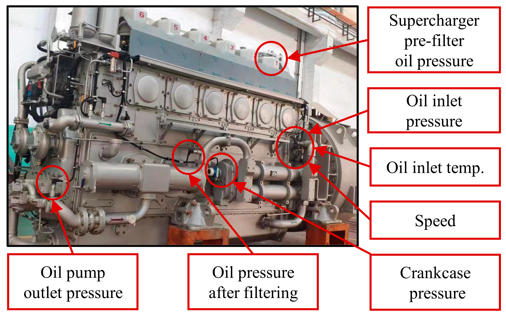
As is widely recognized, the primary function of the lubrication system in a diesel engine is to reduce the wear of components, decrease frictional work, and achieve the cooling and cleaning of the lubricated surfaces. The oil pump raises the lubricating oil to sufficient pressure and forces it to the friction pairs of internal components, ensuring that all the moving friction pairs within the diesel engine are adequately lubricated. Subsequently, the lubricating oil flows back to the oil pan under the force of gravity. The internal moving friction pairs within the lubrication system are not amenable to direct monitoring, and monitoring points are typically arranged on the off-board piping of the engine, as shown in Figure 6 and Figure 7 presents the lubrication system sensor measurement points.

Some scholars have managed to detect failures in external components through the monitoring points on the external lubrication piping of engines. This includes detecting leaks in oil pipelines, the wear of oil pumps, and faults in heat exchangers or filters. However, monitoring the internal lubrication conditions of diesel engines remains a significant challenge. Internal lubrication in a diesel engine is a complex system crucial for fault diagnosis. Abnormal wear or high temperatures in internal moving friction pairs can cause considerable damage to the engine. The lubrication state at the friction surfaces depends on the friction pairs’ operational state and the lubricating oil’s viscosity. Appropriate lubricating oil viscosity can produce an oil film thickness that protects the moving parts. Given that current monitoring capabilities are limited to measuring external pipeline temperatures and pressures, this discussion aims to analyze the internal operational state of the diesel engine based on parameters from the external piping of the engine’s oil system.

When the pressure relief valve in the piping is closed, the pressure inside the diesel engine is primarily generated by the flow resistance of the lubricating oil [25]. Under this condition, it can be assumed that the lubricating oil flows laminarly in the oil passages, adhering to the Hagen–Poiseuille law [26]:

$$∆\mathrm{p}=\mathrm{Q}\mathsf{\eta }{\displaystyle \frac{8\mathrm{L}}{\mathsf{\pi }{{\mathrm{R}}_1}^4}}$$

(7)

where $∆p$ represents the pressure difference between the two ends of the pipe, $Q$ is the volumetric flow rate, $\eta$ is the dynamic viscosity, $L$ is the length of the pipe, and $R_1$ is the radius of the pipe. When the pipeline structure and the clearance between the friction pairs remain unchanged, it is apparent that variations in the internal pressure of the pipeline are related to the oil flow rate and the oil viscosity. This is more specifically illustrated in Figure 8.

Firstly, as the diesel engine’s rotational speed, power, and torque increase, calculations from the test bench indicate that 6.49% of the total heat generated by the fuel is carried away by the engine oil, leading to a rise in oil temperature. Engine oil viscosity is highly sensitive to temperature changes. The viscosities of oil at 40 °C, 80 °C, and 88 °C were measured and regressed using the Vogel equation based on the observed temperature–viscosity data, as shown in Figure 9.

$$\ln \eta =A_1+{\displaystyle \frac{B_1}{\left(T+C_1\right)}}$$

(8)

$T$ is the temperature and $A_1$, $B_1$, and $C_1$ are constants related to the properties of the oil sample.

According to Figure 9, as the engine oil’s temperature increases, the oil’s viscosity decreases. Consequently, this leads to a reduction in the oil film thickness and oil pressure.

There exists the following relationship between the pump speed and the oil flow rate [27]:

$$\mathrm{Q}=\mathrm{j}\mathsf{\pi }{\mathrm{R}}_2\mathrm{h}{\mathrm{B}}_2\mathrm{n}{10}^{-\mathrm{a}}$$

(9)

In the equation, $Q$ represents the average flow rate, $R_2$ is the pitch circle radius, $h$ is the tooth height, $B_2$ is the tooth width, and $n$ is the rotational speed.

According to the principles of mechanical design, under standard conditions

$${\mathrm{R}}_2={\displaystyle \frac{\mathrm{m}\mathrm{Z}}{2}}$$

(10)

$$\mathrm{h}=\mathrm{m}$$

(11)

$${\mathrm{B}}_2=\mathsf{\beta }\mathrm{m}$$

(12)

where $m$ represents the gear module, $Z$ is the number of teeth, and $\beta$ is the ratio of the tooth width to the module.

Given the constant $A_2=2\mathsf{\pi }\mathsf{\beta }{10}^{-6}$, by rearranging the above formula for the average flow rate, the relationship between the rotational speed and the engine oil flow rate can be derived:

$$\mathrm{Z}={\displaystyle \frac{\mathrm{Q}}{\mathrm{n}{\mathrm{m}}^2{\mathrm{A}}_2}}$$

(13)

The formula shows that the rotational speed and the engine oil flow rate are in direct proportion for a given diesel engine, with all design parameters being constant. As the temperature of the engine oil increases, causing a decrease in density, both factors together can increase the flow rate of the engine oil, ultimately leading to a rise in pressure. It is worth noting that the clearance size of the moving friction pairs also influences the engine oil pressure. The radial clearance of the lubrication system’s friction pairs should be within the range of 0.09 to 0.133 mm. If design errors or assembly mistakes cause the clearance to be outside this reasonable range, there can be significant deviations in engine oil pressure. Overall, the engine’s rotational speed and oil temperature affect the oil pressure value during operation.

4.3. Establish an Adaptive Dynamic Threshold

In this section, we applied the dynamic parameter threshold method introduced in Section 2.2, focusing on the critical parameters identified earlier: the oil inlet temperature and the oil inlet pressure. For different engine rotational speed positions, we utilized four distinct mathematical models for data fitting: the cubic model, the parabola model, the exponential model, and the line model. By establishing fitting curves for each model, we further calculated the coefficient of determination ${\mathrm{R}}^2$ and the RSS metrics to assess the fitting effectiveness and select the optimal fitting model.

This process aims to determine which mathematical model most accurately describes the relationship between the oil inlet temperature, the oil inlet pressure, and the engine rotational speed, thereby providing a solid theoretical basis for setting dynamic parameter thresholds. The selection of the optimal model is based on two criteria: the coefficient of determination ${\mathrm{R}}^2$ reflects the model’s ability to explain the variability of the dependent variable, and the RSS measures the deviation between the model’s predicted values and the actual observed values. High ${\mathrm{R}}^2$ values and low RSS values indicate good fitting effectiveness, meaning the model can accurately predict the relationship between parameters. The fitting results are organized and displayed in

Table 9. Fitting results of different models at various rotational speeds for two engines.

Engine ID	Speed (RPM)	Fitting Model	Fitting Formula	${\mathit{R}}^2$	RSS
1#	400	Cubic	$y=0.005x^3-0.64x^2+20.5x+217.7$	0.95	1.03 × 107
		Parabola	$y=0.13x^2-19.7x+907.2$	0.95	1.05 × 107
		Exponential	$y=897.5·{\mathrm{e}}^{-0.03\mathrm{x}}$	0.95	1.09 × 107
		Line	$y=-5.9x+546.7$	0.93	1.68 × 107
	720	Cubic	$y=-0.007x^3+1.5x^2-117.4x+3418$	0.94	8,313,981
		Parabola	$y=0.34x^2-48.5x+2113$	0.94	8,916,979
		Exponential	$y=1527·{\mathrm{e}}^{-0.02\mathrm{x}}$	0.93	9,395,081
		Line	$y=-9.14x+972.2$	0.9	1.41 × 107
	840	Cubic	$y=0.009x^3-1.5x^2+66.9x-161.8$	0.94	6.91 × 107
		Parabola	$y=0.17x^2-29.6x+1673$	0.93	7.42 × 107
		Exponential	$y=1595·{\mathrm{e}}^{-0.02\mathrm{x}}$	0.93	7.60 × 107
		Line	$y=-5.9x+546.7$	0.91	9.22 × 107
	1000	Cubic	$y=0.01x^3-5.9x^2+359x-6483$	0.9	7,113,571
		Parabola	$y=0.29x^2-51.25x+2591$	0.87	8,884,480
		Exponential	$y=2663·{\mathrm{e}}^{-0.03\mathrm{x}}$	0.87	8,903,469
		Line	$y=-12.27x+1295$	0.87	8,995,574
2#	400	Cubic	$y=0.004x^3-0.57x^2+16.5x+316.2$	0.96	5.76 × 106
		Parabola	$y=0.1x^2-16.7x+846.1$	0.96	6.20 × 106
		Exponential	$y=961.8·{\mathrm{e}}^{-0.03\mathrm{x}}$	0.96	6.38 × 106
		Line	$y=-6.8x+603.2$	0.95	8.51 × 106
	720	Cubic	$y=-0.004x^3+1.07x^2-96.3x+3328$	0.96	7,005,293
		Parabola	$y=0.4x^2-59.3x+2659$	0.96	7,057,648
		Exponential	$y=2368·{\mathrm{e}}^{-0.02\mathrm{x}}$	0.96	7,080,272
		Line	$y=-14.74x+1432$	0.93	1.44 × 107
	840	Cubic	$y=0.008x^3-1.1x^2+40.6x-230.4$	0.94	9.27 × 107
		Parabola	$y=0.17x^2-31.9x+1817$	0.94	9.47 × 107
		Exponential	$y=1768·{\mathrm{e}}^{-0.02\mathrm{x}}$	0.93	9.60 × 107
		Line	$y=-10.8x+1200$	0.92	1.15 × 108
	1000	Cubic	$y=0.004x^3-0.9x^2+46.3x+116$	1	1.81
		Parabola	$y=0.26x^2-58.63x+2$251	1	4428.7
		Exponential	$y=2130·{\mathrm{e}}^{-0.02\mathrm{x}}$	1	4748.46
		Line	$y=-12.04x+1359$	1	15,545.82

.

As shown in Figure 10, by plotting the four fitting models for a single condition and performing a summary analysis of all the fitting models and fitting accuracy, it was found that after comparing the four models (cubic, parabola, exponential, and line), the cubic fitting model achieved higher coefficients of determination $R^2$ and lower SSE across all four rotational speed positions for both engines, demonstrating superior fitting performance in almost all cases. This indicates that the cubic model can more accurately capture the complex nonlinear relationship between the oil inlet temperature, the oil inlet pressure, and the engine rotational speed.

To further validate this fitting result’s reliability and predictive accuracy, the next step involves plotting the optimal fitting model graphs for the two engines at various rotational speeds, along with the 99% prediction intervals and residual statistics charts.

Table 10. Optimal fitting model parameters.

No.	Parameter Name	Parameter Content
1	oil inlet temperature	the X-axis
2	oil inlet pressure	the Y-axis
3	rotational speed	400 rpm/720 rpm/ 840 rpm/1000 rpm
4	prediction interval	99%
5	fit group	regression models
6	fit category	cubic

shows the parameter information of the fitting model.

As can be seen from the Figure 11 and Figure 12, although the two diesel engines exhibit similarities in various aspects, there are still subtle differences in the fitted models due to factors such as assembly processes, component quality, or fuel quality. Therefore, there is no absolute standard model for fault diagnosis in the diesel lubrication system. The adaptive threshold diagnosis method we propose is based on the operational characteristics of each diesel engine, enabling self-correction and the evaluation of the model throughout its entire life cycle.

Specifically, across various gear positions, we observed that the oil inlet pressure tends to decrease with an increase in temperature. This trend suggests that the decrease in oil pressure could be due to a reduction in the viscosity of the lubricating oil as its temperature rises. When the dataset is sufficient, the distribution of residuals for the oil inlet pressure conforms to a normal distribution, indicating the adaptability of the model fitting and the consistency of predictions. However, for Engine #2, the residual distribution exhibited an unusual bimodal characteristic under the condition of 1000 RPM due to limited data. Such a bimodal distribution might indicate the presence of two distinct operational modes at this specific rotational speed or reflect some form of systematic bias in the data collection process. These findings underscore the importance of considering the interplay among the rotational speed, the inlet oil temperature, and the inlet oil pressure when conducting engine fault detection.

4.4. Fault Data Validation

To validate the effectiveness of the proposed approach, fault detection was conducted on Dataset B, which contains fault data collected from the lubrication system failure tests described in Section 3.2. This study’s method was compared with current mainstream fault detection algorithms, covering supervised and unsupervised learning algorithms. The specific supervised learning algorithms compared include the MLP, RF, SVM, and XGBoost models, and the unsupervised learning algorithms include the LOF and IF models.

A notable advantage of this study’s model is that it does not require fault data for the training phase. Therefore, different training data configurations were adopted to fairly evaluate the performance of the supervised learning algorithms, involving training these algorithms with 0.1%, 1%, and 10% of the fault data. This configuration aims to explore the performance of supervised learning algorithms at varying levels of fault data availability and to test the superiority of the method proposed in this paper in fault detection tasks.

According to the method described in this paper, we can utilize data from a healthy state diesel engine to construct an adaptive threshold for the oil inlet pressure at 1000 RPM. The plotting data collected under fault conditions showed that many data points exceeded the established threshold range. This phenomenon validates the practicality of the proposed method in effectively capturing lubrication system faults.

Based on the analysis results presented in

Table 11. The MIC of all parameters with the oil inlet temperature.

Oil Inlet Pressure	Oil Outlet Pressure	Pre-Supercharger Oil Pressure Before Filter	Post-Supercharger Oil Pressure Before Filter
0.728	0.539	0.557	0.418

, for Dataset B, the most significant correlation is observed between the oil inlet pressure and the oil inlet temperature, where the MIC score reached 0.728. Furthermore, as indicated by the data in

Table 12. Fitting results with different models.

Fitting Model	${\mathit{R}}^2$	RSS
Cubic	0.88	4,725,577.52
Parabola	0.88	4,785,478.32
Exponential	0.88	4,855,222.63
Line	0.85	6,172,648.81

, the optimal model fitting choice is identified as the cubic polynomial model when employing the adaptive dynamic threshold construction method. The model’s $R^2$ and RSS are 0.88 and 4,725,577, respectively, demonstrating the model’s superior fitting performance and prediction accuracy.

Figure 13 intuitively displays the distribution of the normal and faulty samples and the threshold intervals determined by those above the optimal fitting model. This visual representation reveals the model’s effectiveness in distinguishing between samples in different states and provides a powerful tool and basis for further fault diagnosis and health monitoring. The success of this method lies in its ability to fully utilize data from normal operating conditions by constructing adaptive thresholds to delineate the normal operational range of the system. When a fault occurs, relevant parameters (such as the oil inlet pressure) will exhibit significant deviations from the normal range, triggering a fault alarm. This approach to building thresholds based on health state data is particularly suitable for practical application scenarios where fault data are challenging to obtain or completely absent.

Currently, most domestic medium-speed diesel engine manufacturers use fixed alarm values for threshold monitoring at monitoring points. Each monitoring sensor has its own unique alarm point, unload point, or shutdown point. Based on the fault data in Figure 13, under the operating condition of 1000 rpm, the oil inlet temperature is approximately 63–67 °C, and the oil inlet pressure is around 600–750 kPa. According to the alarm points, unload points, and shutdown points in Table 3, the existing fixed threshold monitoring method does not trigger any alerts. However, using the dynamic threshold alarm method proposed in this paper, it is evident that a fault has already occurred within the diesel engine lubrication system. Inspection after disassembly confirmed that the diesel engine has experienced mild bearing wear.

It can be seen from the test parameters in

Table 13. Key information for the experiment.

Dataset ID	State of Health	Parameter Type	Speed/RPM
${\mathit{X}}_3$	Normal	5	1000
	Fault	5	1000

and the data in

Table 14. Comparison of fault detection performance across different models.

Model Type	Proportion of Fault Samples Used for Training	Model	Acc	Recall	F1	FNR	FPR
unsupervised	0%	IF	0.797	0.785	0.800	0.215	0.192
		LOF	0.910	0.890	0.910	0.11	0.067
		Proposed Method	0.920	0.820	0.920	0.18	0.0005
supervised	0.1%	MLP	0.810	0.626	0.770	0.374	0
		RF	0.744	0.489	0.657	0.511	0
		SVM	0.764	0.528	0.691	0.472	0
		XGBoost	0.729	0.457	0.628	0.543	0
	1%	MLP	0.963	0.927	0.962	0.073	0
		RF	0.950	0.900	0.947	0.1	0
		SVM	0.952	0.903	0.949	0.097	0
		XGBoost	0.968	0.935	0.967	0.065	0
	10%	MLP	0.995	0.990	0.995	0.01	0
		RF	0.996	0.992	0.996	0.008	0
		SVM	0.997	0.994	0.997	0.006	0
		XGBoost	0.995	0.990	0.995	0.01	0

that the method proposed in this study significantly outperforms the IF and LOF algorithms regarding fault detection performance. Although supervised learning models can achieve high diagnostic accuracy with an abundance of fault samples, their performance in detecting faults dramatically decreases in environments where fault samples are scarce, rendering them inadequate for practical application requirements. Among them, it can be observed that the false positive rate of the supervised learning algorithms is 0. The main reason for this is the issue of data imbalance. During training, the data for healthy conditions significantly outweighs that for fault conditions, causing the model to be more inclined to classify the equipment as being in a healthy state during inference.

4.5. Method Application

During the model fitting process, the confidence interval of the predicted boundary is calculated, which consists of two confidence boundary curves. When the monitoring data points fall within the confidence interval, it indicates that the lubrication system is operating normally. If the total number of monitoring data points exceeds a certain percentage of the confidence interval over a monitoring cycle, the system will issue an alarm.

Just as abnormal blood indicators in humans change with age, we believe that diesel engines also exhibit a weakening of indicators as their life cycle extends. Therefore, the system fitting model needs to change along with the life cycle of the diesel engine. In practical engineering applications, it is essential to dynamically update the fitting model and confidence interval in cycles using the dynamic threshold monitoring method, allowing for the timely observation of faults and trends. Specifically, we first perform self-learning on the data from the diesel engine’s healthy state to fit the current “standard model”. Then, we use the collected short-term, medium-term, and long-term datasets for the diagnostic evaluation of the system. The short-term dataset primarily diagnoses in conjunction with the confidence interval of the “standard model”, the medium-term dataset conducts a trend analysis by comparing the fitted model with the parameters of the “standard model”, and the long-term model focuses on correcting the model after the performance of the “standard model” has weakened.

5. Conclusions

This paper combines the relative advantages of data mining methods and threshold techniques, proposing an adaptive threshold construction method based on dynamic parameter relationship inference. The main conclusions are as follows:

• Utilizing the method of dynamic parameter relationship inference, clear correlations among numerous parameters, such as the engine speed, the inlet temperature, and the inlet oil pressure, were identified.
• Theoretical analysis and formula derivation have proven that the engine speed and the oil flow rate are directly proportional to a diesel engine with specified design parameters. As the temperature increases, causing a decrease in oil density, the oil pressure will decrease.
• Data collected from fault experiments have demonstrated that the adaptive threshold method proposed in this paper can effectively identify ship faults. Especially in scenarios where fault samples are scarce, this method significantly outperforms static threshold methods and machine learning approaches in performance.