Article

Road Roughness Recognition: Feature Extraction and Speed-Adaptive Classification Based on Simulation and Real-Vehicle Tests

1
College of Automobile and Traffic Engineering, Nanjing Forestry University, Nanjing 210037, China
2
School of Engineering and Materials Science, Queen Mary University of London, Mile End Road, London E1 4NS, UK
*
Author to whom correspondence should be addressed.
Machines 2025, 13(5), 391; https://doi.org/10.3390/machines13050391
Submission received: 24 March 2025 / Revised: 28 April 2025 / Accepted: 6 May 2025 / Published: 8 May 2025
(This article belongs to the Special Issue Advances in Vehicle Suspension System Optimization and Control)

Abstract

Road roughness exerts a direct influence on the vertical dynamic performance of vehicles, and the accurate characterization of road roughness is essential for optimizing vehicle suspension systems. This paper addresses two key challenges in roughness recognition: feature extraction and adaptive classification under different speeds. In detail, based on simulation tests of the quarter-vehicle vertical vibration model and real-vehicle test, this paper reveals the strong correlation between the unsprung mass vertical vibration response of vehicles and road roughness. The feasibility of using unsprung mass vertical vibration response as a feature for recognizing and classifying road roughness is verified. And an adaptive road roughness classifier is proposed based on vehicle-speed-related features. Both simulation and real-vehicle results confirm that (i) the unsprung vertical vibration displacement is strongly correlated with road roughness (R2 = 0.997); (ii) road roughness can be classified with high accuracy with the unsprung mass vertical vibration response taken as the only feature (simulation tests: 98.88% to 100%; real-vehicle tests: 100%); and (iii) the accuracy of the proposed speed-adaptive classifier is 20% more accurate than the conventional classifier that does not consider vehicle speed features. This research can provide accurate road excitation for the adaptive real-time control of semi-active or active vehicle suspensions.

1. Introduction

Off-road vehicle (ORV) refers to vehicles that are designed and manufactured for good driving performance on unstructured road surfaces (soil, sand, snow, etc.), which have a wide range of applications in military transport [1], agricultural farming [2], engineering operations [3], desert energy development [4], and planetary exploration [5]. ORVs always have low driving speeds, e.g., the working speed of agricultural and forestry operation vehicles ranges between 4 km/h and 12 km/h [6]. Paper [7] points out that despite low driving speeds, the vertical excitation that agricultural and forestry operation vehicles receive is several times that of ordinary vehicles. If the vehicle can sense the information of the current road surface, it can make appropriate adjustments to the parameters of each control subsystem of the chassis in order to obtain better pass performance, smoothness, and maneuvering stability, etc. [8,9,10,11].
There are two main common ways to obtain road roughness information, namely road roughness measurement and road roughness recognition [12]. Road roughness measurement is defined as the application of various types of measuring equipment to obtain specific elevation information of roads; road roughness recognition is defined as the use of certain algorithms to classify road roughness using the vehicle vertical vibration response. Among them, the measurement approaches are mainly classified into contact measurement and non-contact measurement [13]. The contact measurement approaches have high measurement accuracy. However, their measurement efficiency is relatively low. The road roughness signal measured by non-contact measurement approaches has less error, but there is the problem of high measurement costs. In addition, non-contact measurement is easily interfered with by the external environment [14,15,16]. The vehicle-response-based road roughness recognition [17,18,19] is one non-contact measurement approach. It does not require the installation of various types of complex sensors and only needs on-board sensors to obtain the road surface excitation during vehicle traveling. Such an approach is convenient to integrate into the chassis domain system of the vehicle. It is worth noting that the road roughness information obtained through the vehicle-response-based approach does not represent the actual road surface profile. Instead, it reflects the real-time elevation displacement of the as experienced by the wheel during its interaction with the surface. This is defined as the effective roughness of the road [20], which focuses on the road’s influence on the vehicle during real-world driving.
The non-contact road roughness recognition approaches can be categorized as model-based and data-driven, depending on how the relationship between road roughness and vehicle vibration response is established [21]. Model-based recognition requires knowledge of the vehicle model parameters and uses vehicle body responses to identify road roughness. In contrast, data-driven recognition does not rely on an established vehicle model. Instead, it uses pre-collected data to fit a mapping relationship between road roughness and vehicle vertical vibration responses through algorithms such as neural networks. Road roughness data are then identified using the trained neural network model.
To obtain accurate road roughness information, extensive studies have been con-ducted. For instance, Z. Li et al. [22] proposed identifying road roughness using features such as the total variation, variance, and resonance peak amplitude of wheel forces. J. Li et al. [23] evaluated various neural network models in a simulation environment for road roughness recognition, demonstrating that the Nonlinear auto-regressive external input neural network model yielded the best results. L. Liu et al. [24] designed a novel Kalman filter that incorporates vehicle longitudinal acceleration to identify road roughness. This new Kalman filter achieves higher recognition accuracy under non-uniform speed conditions, urban driving scenarios, and braking conditions compared to traditional Kalman filters. S. Li et al. [25] developed a road roughness recognition algorithm based on genetic algorithm-optimized long- and short-term memory neural network adaptive Kalman filtering, which is capable of quickly and accurately identifying and grading road roughness. Compared to traditional Kalman filtering algorithms, this GA-LSTM-based adaptive approach showed superior adaptability to complex conditions. K. Chen et al. [26] utilized the Relief-RBF algorithm to extract key features of road roughness and constructed a radial basis function (RBF) neural network-based classifier for road roughness grading and identification, demonstrating strong robustness in experimental results. Rahman [27] developed an optimal Kalman estimator that uses vertical accelerations of the sprung and unsprung masses to back-calculate road roughness. Fergani et al. [28] built a nonlinear algebraic observer based on unknown inputs for road roughness recognition and validated their results using ISO-standard graded roads through simulations. Imine et al. [29] employed a four-degree-of-freedom half-car model to construct second-order and third-order sliding mode observers for road roughness recognition. Comparisons with LPA profilometer measurements showed high precision in short-wavelength recognition but limitations in long-wavelength recognition. M. Doumiati et al. [30] applied an adaptive Euler-Cauchy parameter observer for road profile estimation, with experimental results confirming its effectiveness through comparisons with actual profilometer measurements. Yazan Ibrahim Alatoom et al. [31] collected road data using smartphones and predicted international roughness index (IRI) with neural network models. Their findings demonstrated that artificial neural network models achieved high accuracy in IRI prediction.
The aforementioned studies still face several key unresolved issues. First, most research focuses on well-maintained, hard road surfaces, with limited recognition methods for specialized road environments such as soft soils. Second, although machine learning techniques demonstrate excellent recognition accuracy, the excessive number of features still presents significant challenges in practical applications and limits their scalability. Third, vehicle vertical responses are closely related to changes in vehicle speed, yet existing studies often consider a single speed and fail to adequately account for the impact of speed variations on road excitation energy, leading to limitations in road excitation recognition. To address these issues, this paper proposes a method for constructing a speed-adaptive road roughness classifier that incorporates vehicle speed features. The strong relationship between unsprung mass vibration responses and road roughness is revealed. Moreover, by combining a speed-adaptive mechanism, the proposed method significantly improves the accuracy and robustness of the recognition system. Through theoretical analysis, simulations, and real data validation, it is demonstrated that by considering vehicle speed, high-precision road roughness classification can be achieved under various speed conditions using only unsprung mass vertical vibration responses as features.

2. Materials and Methods

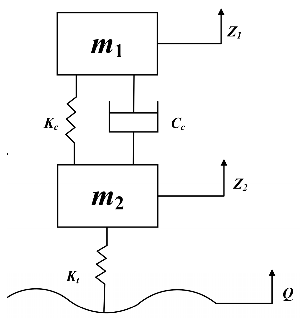
2.1. Simulation of Vehicle Model

In order to analyze the relationship between unsprung mass vertical vibration response of ORVs and the roughness information of roads where the vehicles are traveling, this paper uses a widely used single-wheel model of a two-degree-of-freedom quarter vehicle (Figure 1), which provides an understanding of the most basic features of the vertical behavior of the vehicle.
Rajamani [32] analyzed the full-car model and its response to road irregularities, demonstrating that the suspension system can be independently designed for each wheel. This indicates that a quarter-car suspension model is sufficient for studying and designing vehicle suspension systems to optimize vertical responses to road irregularities. Assuming that the wheel rolls without slipping or loss of contact, the dynamic equations are as follows:
m 1 z 1 = K c ( z 2 z 1 ) + C c ( z 2 z 1 ) m 2 z 2 = K c ( z 1 z 2 ) + C c ( z 1 z 2 ) + K t ( z 2 Q )
where m1 represents sprung mass; m2 represents unsprung mass; Kc represents suspension stiffness; Cc represents suspension damping coefficient; Kt represents tire stiffness; and Q represents road excitation.
The quarter-vehicle model was implemented in the MATLAB/Simulink 2019b environment, with primary parameters derived from the actual vehicle measurements. The detailed parameters are presented in Table 1.

2.2. Simulation of Road Roughness Signal

The filtered white noise method [33], harmonic superposition method [34], inverse Fourier transform method [35], and time series modeling method are all methodological approaches for simulating road roughness signals in the time domain and establishing road surface models. Among them, the filtered white noise method converts appropriate white noise signals into time-domain road roughness representations, which has been predominantly employed by researchers for constructing time-domain models of road surfaces. Therefore, the filtered white noise method is also used in this paper to simulate road roughness signal. The classical formula for constructing a time domain model of road roughness is shown in Equation (2):
q ˙ ( t ) = 2 π n 1 v q ( t ) + 2 π n 0 G q ( n 0 ) v w ( t )
where q ˙ ( t ) represents time derivative of road roughness signal; q ( t ) represents time-domain signal of the road roughness; v represents vehicle speed; G q ( n 0 ) represents road power spectral density values; n 0 represents reference spatial frequency (usually taken as 0.1 m−1); n 1 represents the road cutoff spatial frequency (usually taken as 0.01 m−1); and w ( t ) represents white noise per unit intensity. Among them, G q ( n 0 ) determines the road grade level, the specific numerical values can refer to the international standard ISO 8608:2016 [36] (namely, “mechanical vibration—road surface profiles—reporting of measured data”), and the details are shown in Table 2.

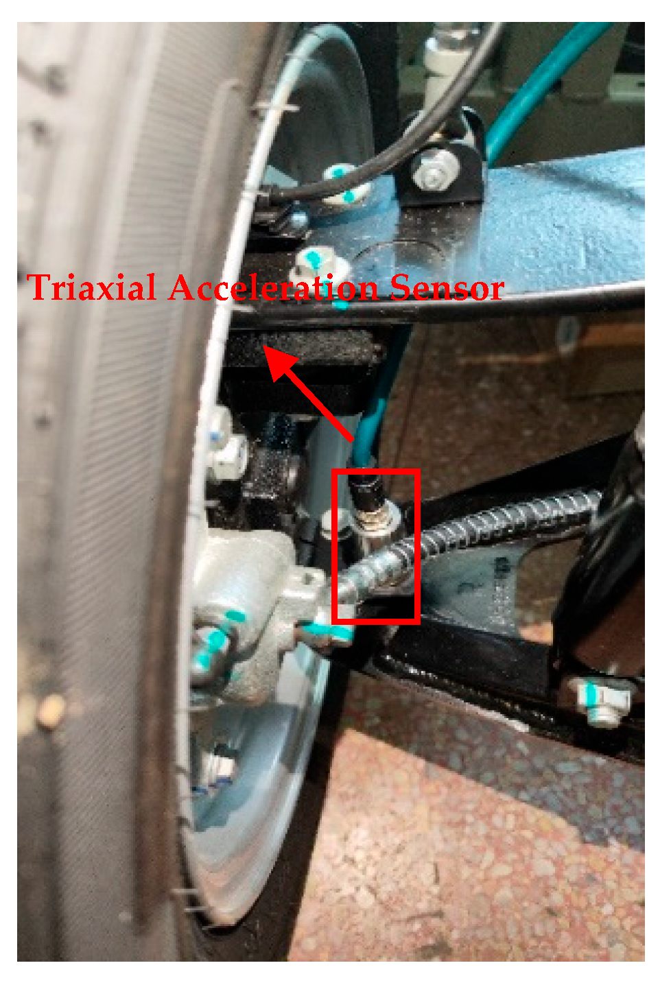
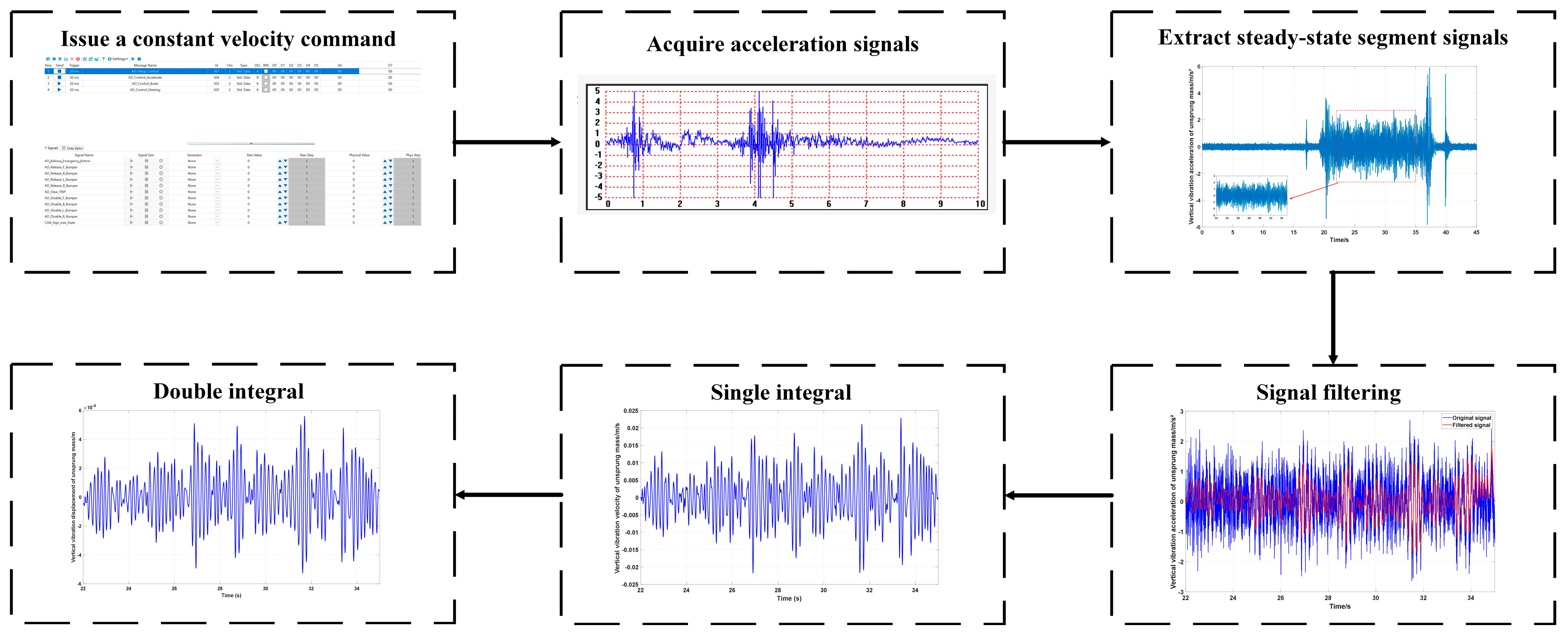
2.3. Construction of Actual Experimental Platform

To validate the accuracy of the simulation results, a triaxial vibration acceleration sensor (VTall-T163E-A, Hunan, China) was installed at the center of the vehicle’s front wheels (both left and right) to measure the vertical vibration response of the wheels. Considering the operational environment of the sensor in vehicle-mounted experiments—such as temperature, waterproofing, and anti-interference capabilities—the selection of the sensor is particularly critical, as it directly affects the precision of data acquisition. The technical specifications of the accelerometer are listed in Table 3.
To ensure accurate measurement of the unsprung mass vertical vibration response, an external mounting bracket was designed at the wheel position. The bracket is equipped with a positioning module, which prevents lateral and longitudinal displacement of the vibration sensor during vehicle operation. The setup is shown in Figure 2.
During the experiment, it is necessary to ensure that the vehicle runs at a constant speed. Given that the vehicle cannot maintain a constant speed during the initial starting phase, only the steady-state portion of the collected signals was analyzed. It is worth noting that even when the steady-state segment of the vehicle speed is selected, the process of double integration of the acceleration signal is still vulnerable to the interference of low-frequency noise and sensor zero drift [37]. When performing double numerical integration on the acceleration signal, even a tiny amount of noise may be amplified and accumulated during the integration process, leading to significant errors, which in turn affects the accurate estimation of the vertical displacement of the wheel or road roughness. Therefore, before integrating the acceleration signal, it is necessary to conduct routine signal preprocessing such as filtering and detrending on the collected original signal. Only after completing these preprocessing steps can the vertical vibration displacement of the wheel center during the vehicle’s running be calculated more reliably. The specific acquisition and processing procedures are illustrated in Figure 3.

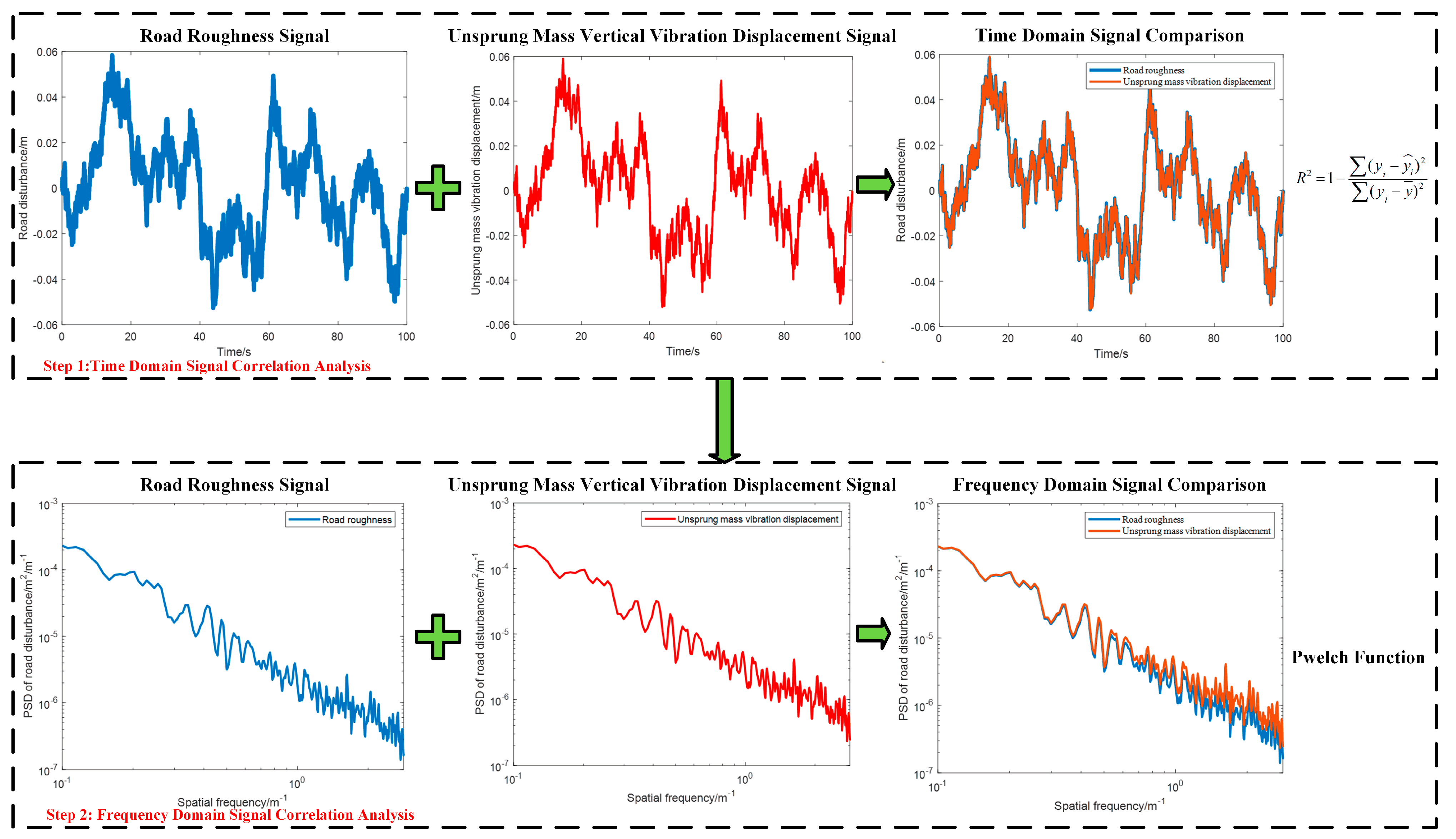
2.4. Signal Consistency Verification Method

Since road roughness signals are the external excitation causing vehicle vibration, the vertical vibration response of the vehicle is closely related to road roughness [38]. To verify the consistency between road roughness signals and vehicle unsprung vibration response signals, this study will adopt a combined time-domain and frequency-domain approach. The specific verification steps are as follows:
Step (1): time-domain correlation analysis
Simulate the road roughness signal and the corresponding unsprung vertical vibration displacement signal of the vehicle using a simulation model. Construct a time-domain comparison plot to visually assess the correlation between the two signals. To quantify the correlation index, this study uses the coefficient of determination (R2) to characterize the time-domain relationship. Generally, an R2 value closer to 1 indicates a stronger linear correlation between the two signals in the time domain. The specific formula for R2 is shown in Equation (3):
R 2 = 1 ( y i y i ^ ) 2 ( y i y ¯ ) 2
where y i represents the simulation of unsprung vertical vibration displacement signal; y i ^ represents simulation of road roughness signal; and y ¯ represents the mean value of y i .
Step (2): frequency-domain correlation analysis
The power spectral density (PSD) of the road roughness and the unsprung mass vertical displacement was estimated using the Pwelch function in MATLAB. The sampling frequency was set to 200 Hz. A Hamming window with a length of 256 samples was applied with a 50% segment overlap (128 samples), and the number of FFT points (NFFT) was set equal to the window length (256).
To obtain the spatial PSD, following the method recommended in ISO 8608:2016, the temporal frequency axis was divided by the vehicle speed (v = 10 km/h = 2.78 m/s), and the corresponding PSD values were multiplied by v. The specific calculation is presented in Equation (4):
G q ( n ) = v G q ( f ) n = f v
where G q ( n ) represents spatial power spectral density (in m2/m−1); v represents vehicle speed (v = 10 km/h = 2.78 m/s); G q ( f ) represents temporal power spectral density (in m2/Hz); f represents temporal frequency; n represents spatial frequency.
If both signals pass time-domain and frequency-domain verifications, they are deemed to exhibit consistency; otherwise, they are considered inconsistent. To clarify the verification workflow, Figure 4 systematically illustrates the signal consistency validation steps.

2.5. Speed-Adaptive Road Roughness Classifier Design Method

Currently, the classifiers used for road recognition mainly include the Support Vector Machine [39] (SVM), K-Nearest Neighbors [40] (KNN), Random Forest [41] (RF), and various neural network models [42]. Reference [43] indicates that four statistical features, namely variance, mean square amplitude, root mean square value, and maximum value, possess good capabilities in recognizing changes in road excitation levels. It is worth noting that the recognition method described in this reference has a high accuracy in recognizing and classifying road surfaces of different levels under the condition of the same vehicle speed. Moreover, there are too many recognition features provided to the classifier, which makes the classification process extremely complex.
On this basis, four statistical features were selected for road roughness recognition in this study: mean absolute value, absolute standard deviation, peak absolute value, and root mean square value. In addition, vehicle speed was input as an additional feature for classifier recognition. The complete steps for the construction of the speed adaptive road roughness classifier are as follows:
Step (1): construct road database for multi-speed conditions
To validate whether the incorporation of vehicle speed can improve the accuracy of the classifier, in this section, filtered white noise is used to construct a database of random roads of Classes A–E under different vehicle speeds (ranging from 5 km/h to 60 km/h, with an equal—difference increment of 5 km/h each time, resulting in a total of 12 speeds). The simulation frequency is set at 200 Hz, and the simulation duration for each speed within each class is 1000 s (for example, the simulation duration of a Class A road at a speed of 5 km/h is 1000 s). With 12 speeds, the total duration amounts to 12,000 s. Therefore, for the five classes, there is a total of 60,000 s of road roughness data. The detailed definition of the road dataset is provided in Table 4.
Step (2): extraction of sample data of unsprung mass vertical vibration response and calculation of statistical features
The above-mentioned road roughness database was input into MATLAB/Simulink 2019b model to obtain the corresponding unsprung mass vertical vibration response. Using a one-second sliding time window (corresponding to 200 data points) [44], the unsprung mass vertical vibration response was extracted as a single sample. For each sample, the mean absolute value (MAV), absolute standard deviation (ASD), peak absolute value (PAV), and root mean square (RMS) were calculated as features for subsequent classification. The calculation formulas for each feature are shown in Equations (5)–(8):
M A V = 1 N i = 1 N x i
A S D = 1 N i = 1 N ( x i x ¯ ) 2
P A V = max ( x 1 , x 2 , x 3 x N )
R M S = 1 N i = 1 N x i 2
where N represents the number of data points in a sample, and here N is taken as 200; xi represents data points of the unsprung mass vertical vibration response; x ¯ represents mean value of the sample data (here is the mean value of 200 data points).
A total of 60,000 samples were constructed from the 60,000 s database. Among them, 6000 samples were used to train the classifier (100 samples were selected for each road grade under 12 different speeds, resulting in 6000 samples for five grades in total), covering all combinations of road grades and speeds; the remaining 54,000 samples were used to evaluate the classifier’s performance.
Step (3): construct speed-adaptive road roughness classifier
The four statistical features (mean absolute value, absolute standard deviation, peak absolute value, and root mean square value) extracted in Step (2) are input into different classifiers for road class identification. Subsequently, vehicle speed as an additional feature (to form five features) was used as input to the classifier, and whether the classification effect of the speed adaptive road roughness classifier was improved with the addition of the speed feature was analyzed by comparison.

3. Results and Discussion

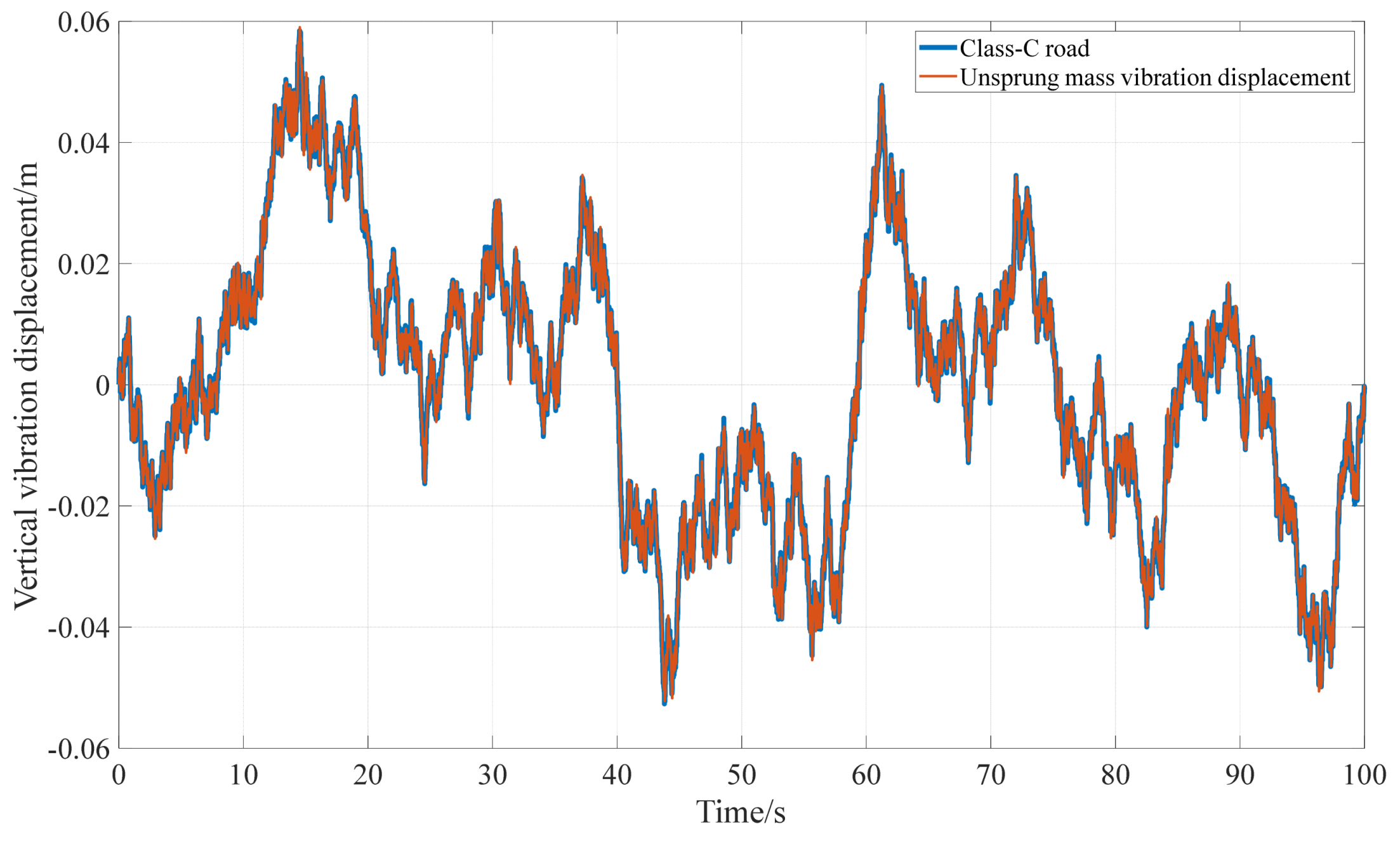
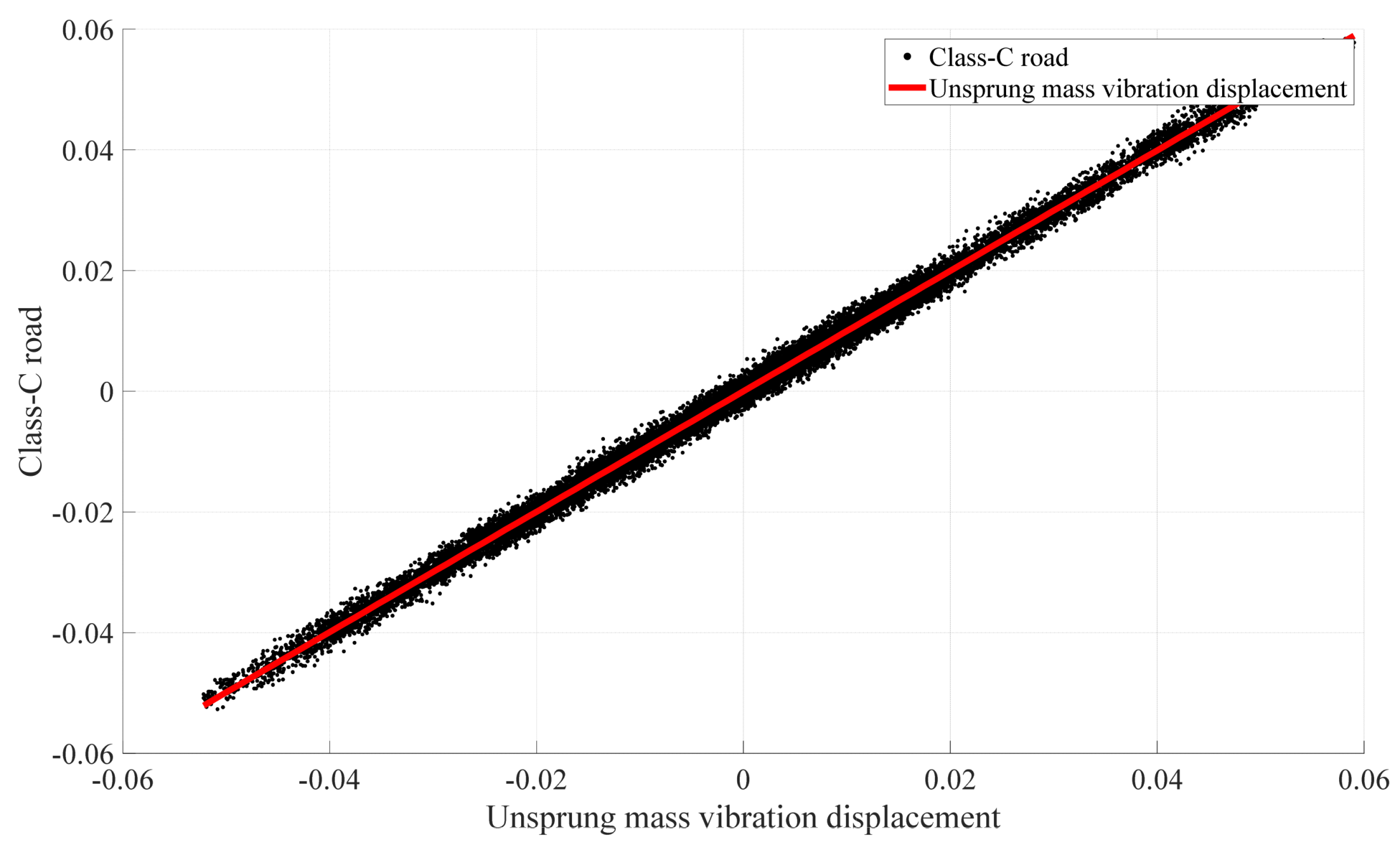
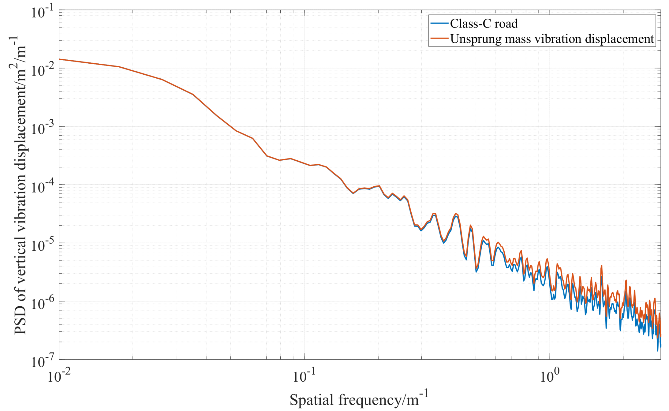
3.1. Time–Frequency Domain Consistency Analysis Based on Theoretical Simulation

To analyze the correlation between the unsprung mass vertical vibration response and road roughness, in the simulation environment, a Class C road surface corresponding to a vehicle speed of 10 km/h is input (the simulation frequency is 200 Hz, and the simulation duration is 100 s, resulting in a total of 20,000 simulation data points). The simulation model outputs the comparison between the Class C road surface and unsprung vertical vibration displacement of the vehicle, as specifically shown in Figure 5.
As shown in Figure 5, the displacement of the unsprung mass vibration demonstrates a high degree of consistency with the input road profile in the time domain. To quantitatively assess their relationship, a correlation analysis was conducted between the unsprung mass vibration displacement and the Class-C road profile. The results indicate a strong correlation, with an R2 value of 0.997, as illustrated in Figure 6.
From Figure 5 and Figure 6, it can be observed that the unsprung mass vibration displacement exhibits a high degree of alignment with the simulated input road profile in the time domain. To further analyze their relationship, the spatial frequency was restricted to the range of 0.01~2.83 m−1. The detailed results within this range are shown in Figure 7.
As shown in Figure 7, the frequency domain of the unsprung mass vibration displacement aligns closely with the frequency domain of the simulated Class-C road profile, remaining within the range defined by the standard power spectral density of a Class-C road. Furthermore, the fluctuation trends of both profiles in this range exhibit strong consistency. This indicates that the vibration displacement of the unsprung mass encapsulates the majority of the characteristics of the road surface traversed by the vehicle, making it a reliable representation of the actual road profile.

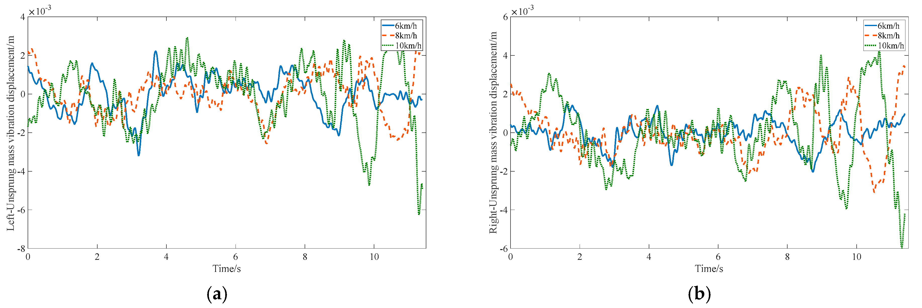
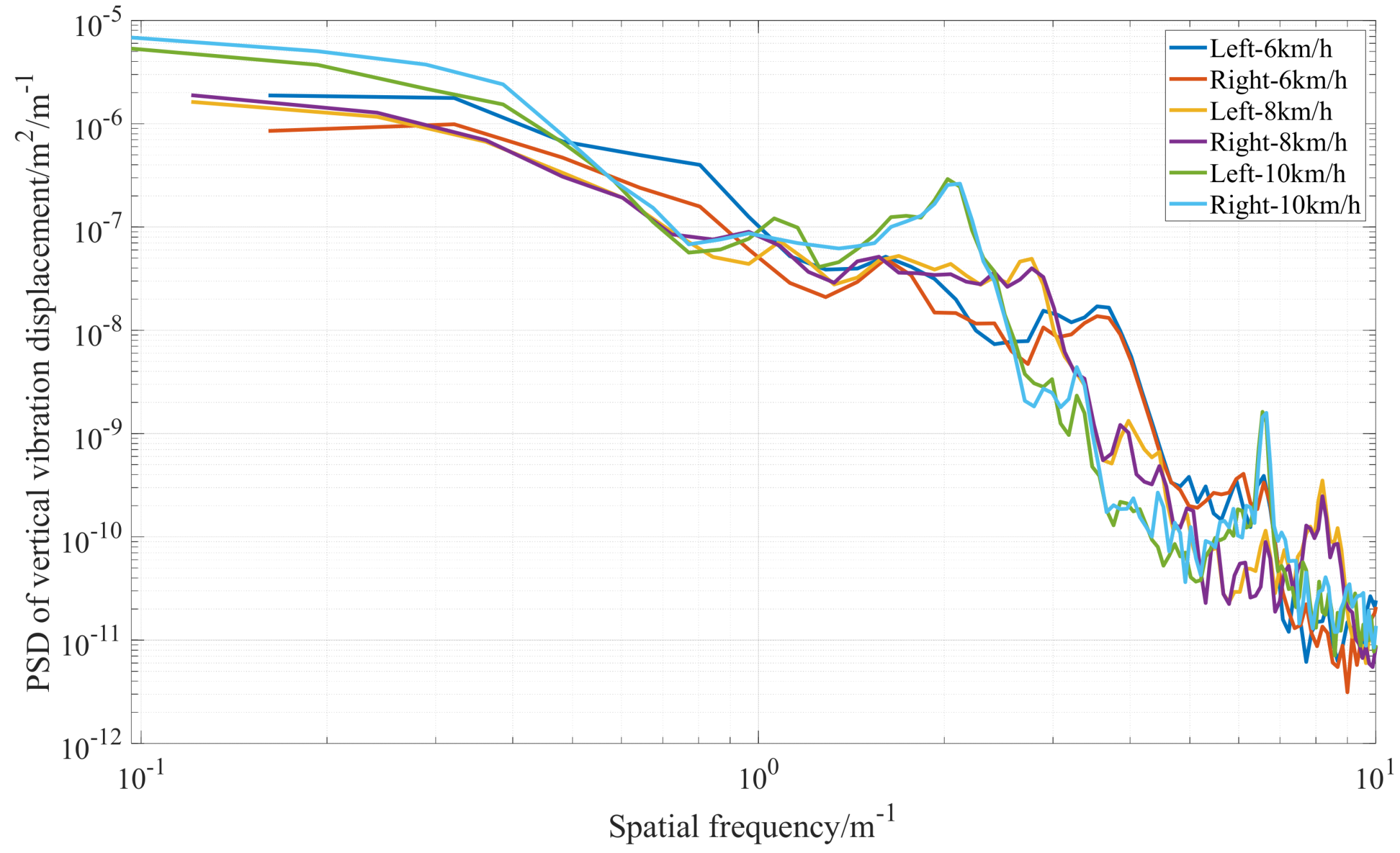
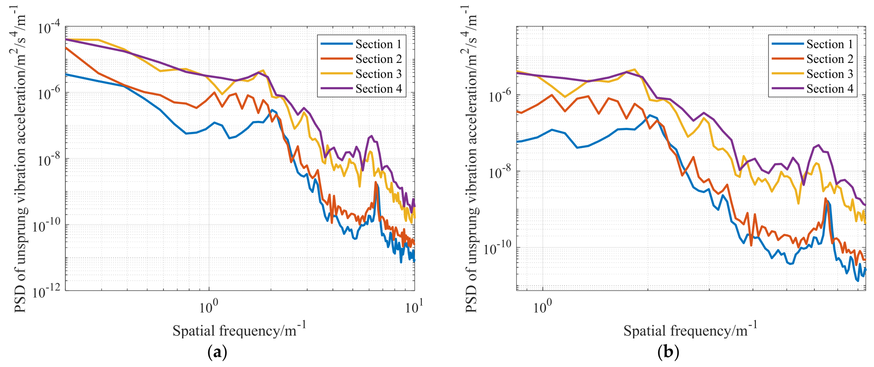
3.2. Consistency Analysis of Left and Right Wheels Based on Real Vehicle Tests

Considering that the commonly used speed range of off-road vehicles is relatively low, in order to conform to the actual application scenarios, constant-speed commands of 6 km/h, 8 km/h, and 10 km/h, respectively, are sent to the vehicle through the upper computer, enabling the vehicle to travel on the same type of road surface at different speeds. The vertical vibration response signals of the unsprung mass of the vehicle are collected. After filtering, the signals are integrated twice to obtain the vertical vibration displacement of the unsprung mass of the vehicle.
The unsprung vertical vibration displacement of the left and right wheels at speeds of 6, 8, and 10 km/h was visualized to represent the time-domain vibration signals at different speeds, as shown in Figure 8.
It can be seen from Figure 8 that under the same test road surface, the unsprung vertical vibration displacement response increases with increasing speeds, which is in line with the actual situation. At different speeds, the trends of the unsprung vertical vibration displacement changes in the time domain of the left-hand wheel and the right-hand wheel have a certain degree of similarity. The time-frequency conversion of the above unsprung sagging vibration displacements of the left and right wheels is shown in Figure 9.
As shown in Figure 9, the unsprung vertical vibration displacements of the left and right wheels exhibit a high degree of consistency in the frequency domain under different speeds. This indicates that the road surfaces traversed by the left and right wheels remain unchanged during vehicle operation. Although there may be of slight deviations in the time-domain unsprung vibration displacements at different speeds, the road surface itself does not vary with the change in vehicle speed. Since road excitation is closely related to the vehicle unsprung vibration displacement, it is feasible to classify and identify the actual road surface traversed by the vehicle based on the unsprung vertical vibration displacement.

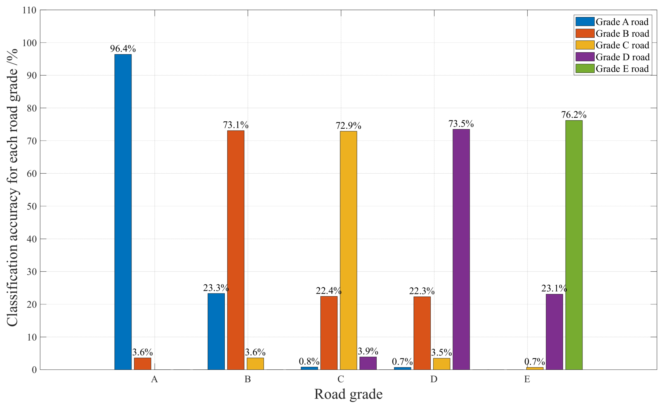
3.3. Construction of Road Roughness Classifier

In this section, the recognition performance of different classifiers is compared. SVM is used to train the aforementioned 6000 sample data, while 54,000 data samples from the original road roughness database are used for testing. Considering the large volume of data, a bar chart illustrating the classification accuracy of the SVM-based road roughness classifier without incorporating the vehicle speed feature is provided for a more detailed analysis, as shown in Figure 10.
As shown in Figure 10, the horizontal axis represents the true road grades in the simulation environment, while the vertical axis indicates the classification accuracy achieved by the classifier for each grade. Each bar, distinguished by color, corresponds to a different road grade (blue: Grade A, red: Grade B, orange: Grade C, purple: Grade D, and green: Grade E). The classification accuracy for each grade is explicitly annotated above the respective bars. Specifically, without the incorporation of vehicle speed feature, the SVM classifier achieves the highest classification accuracy for Grade A road (96.4%), with only a small proportion of samples (3.6%) misclassified as Grade B. For Grades B to E, the classification accuracy significantly decreases, and a common trend is observed: a relatively high misclassification rate between adjacent grades, with approximately 26.9%, 26.3%, 25.8%, and 23.8% of samples misclassified into neighboring grades, respectively. Overall, the SVM classifier achieves a comprehensive classification accuracy of 78.41%.
By repeating the above classification procedure, KNN, Random Forest, and RBF Neural Network were, respectively, employed to classify the entire road roughness dataset. The corresponding bar charts of the classification results for each method are illustrated in Figure 11, Figure 12 and Figure 13, respectively, facilitating a further comparison and evaluation of the performance of different classifiers in the road roughness recognition task.
It is noteworthy that all four classifiers exhibit a certain degree of misclassification between adjacent grades in the medium- and high-grade road surfaces (Grades B to E). To comprehensively characterize the overall classification performance of each classifier, detailed classification accuracy data are presented in Table 5.

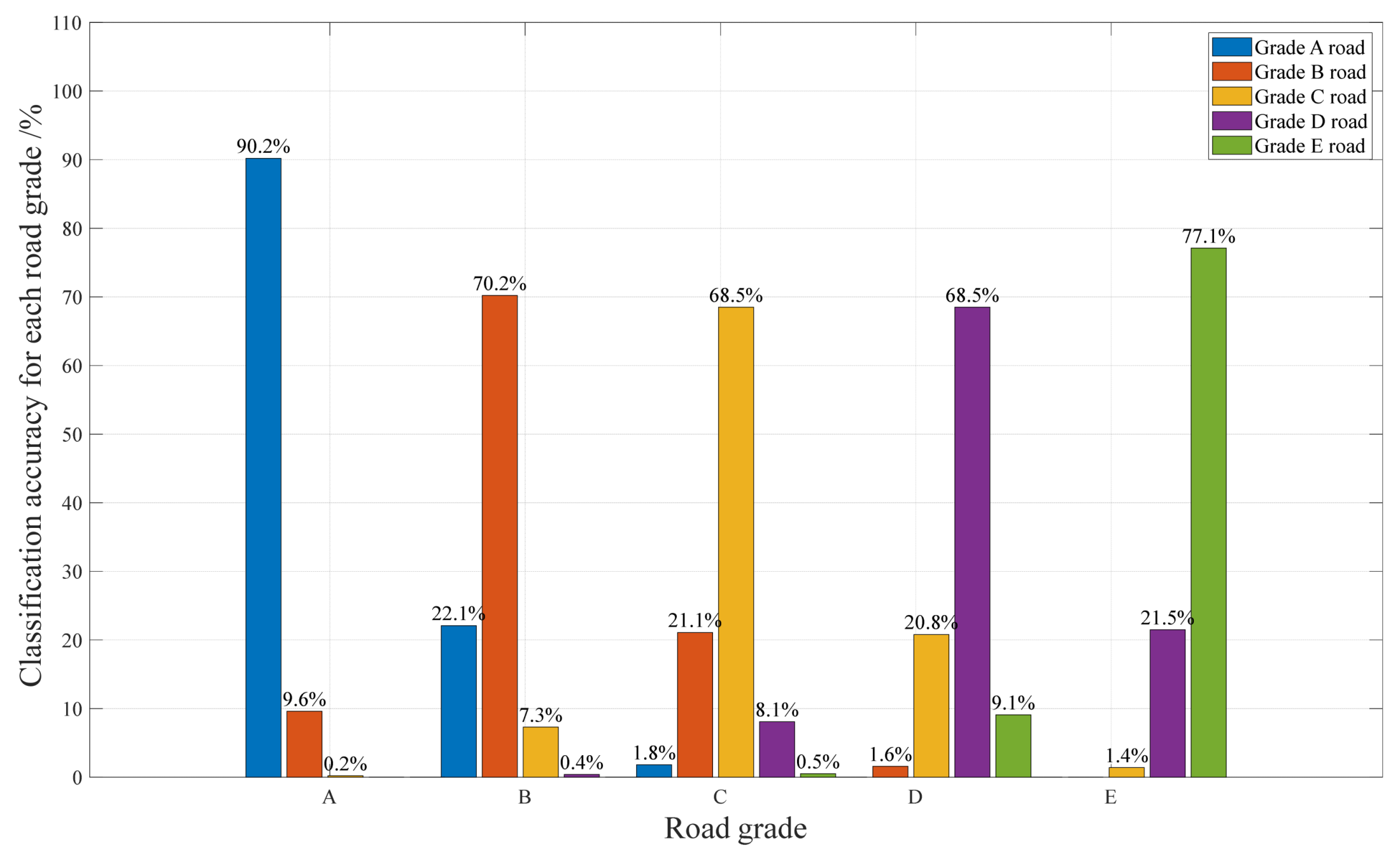
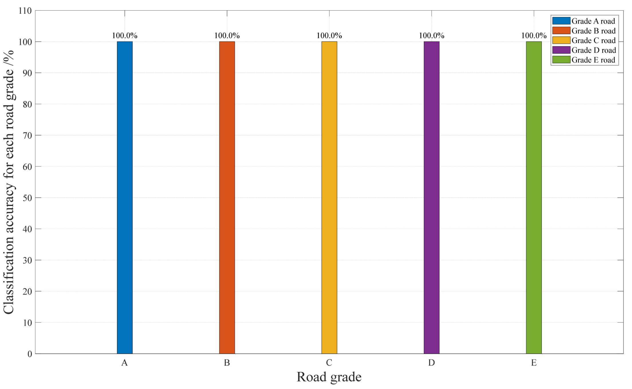
3.4. Construction of Speed-Adaptive Road Roughness Classifier

As discussed in Section 3.3, the classification performance is suboptimal when vehicle speed is not included as an additional feature. To ensure that the classification system performs well across various speeds, this section incorporates vehicle speed as an additional feature, combining it with the four features from Section 3.3. The same classifiers were employed to evaluate the performance, using identical data segments to assess the impact of including vehicle speed. The specific classification results are shown in Figure 14, Figure 15, Figure 16 and Figure 17.
After incorporating vehicle speed as an additional feature, the classification and recognition accuracies of all four classifiers improved significantly, with the average accuracy of each classifier exceeding 99%. The overall classification accuracies of each classifier are presented in Table 6.
As shown in Table 6, the proposed speed-adaptive road roughness classifier improves recognition accuracy by about 20% compared to conventional classifiers, with the KNN-based model achieving the highest accuracy of 100%. However, limited onboard computational power makes real-time calculation of the four statistical features difficult. To enhance recognition efficiency, vehicle speed is fixed as a feature and combined individually with each statistical feature to identify the most effective one. The KNN-based speed-adaptive classifier is still used, and the corresponding accuracies are shown in Figure 18, Figure 19, Figure 20 and Figure 21.
As shown in Figure 18, Figure 19, Figure 20 and Figure 21, as long as vehicle speed is included as a fixed feature, the classification accuracy of road roughness identification is not significantly affected, even with a reduction in the number of the other four statistical features. The specific classification accuracies for different feature selections are summarized in Table 7.

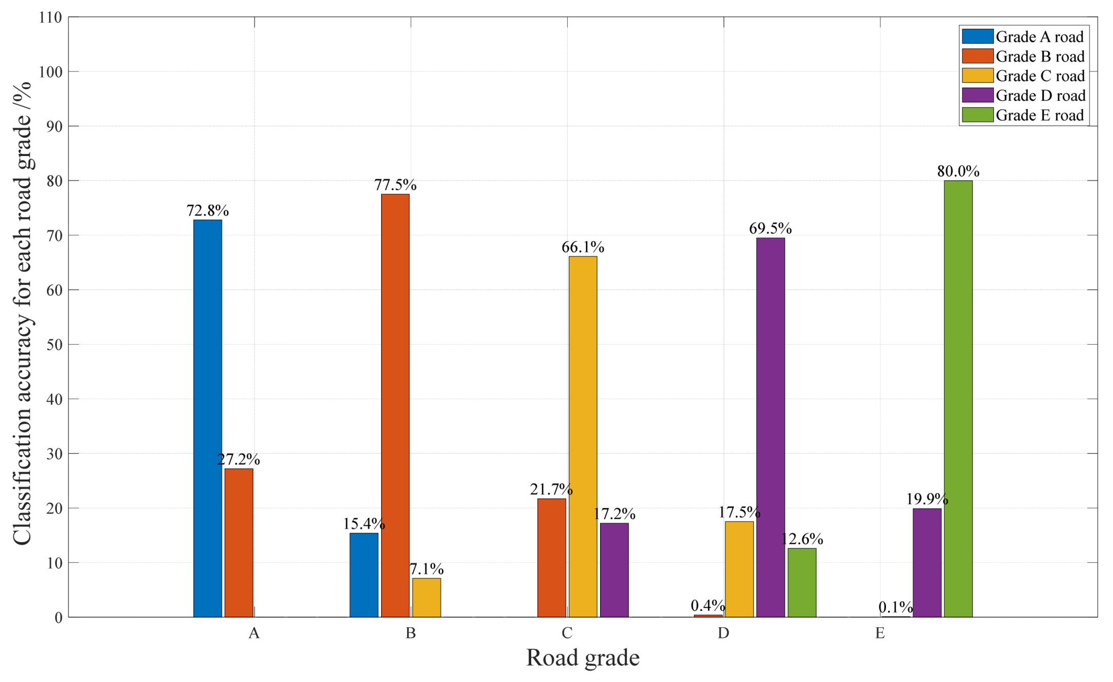
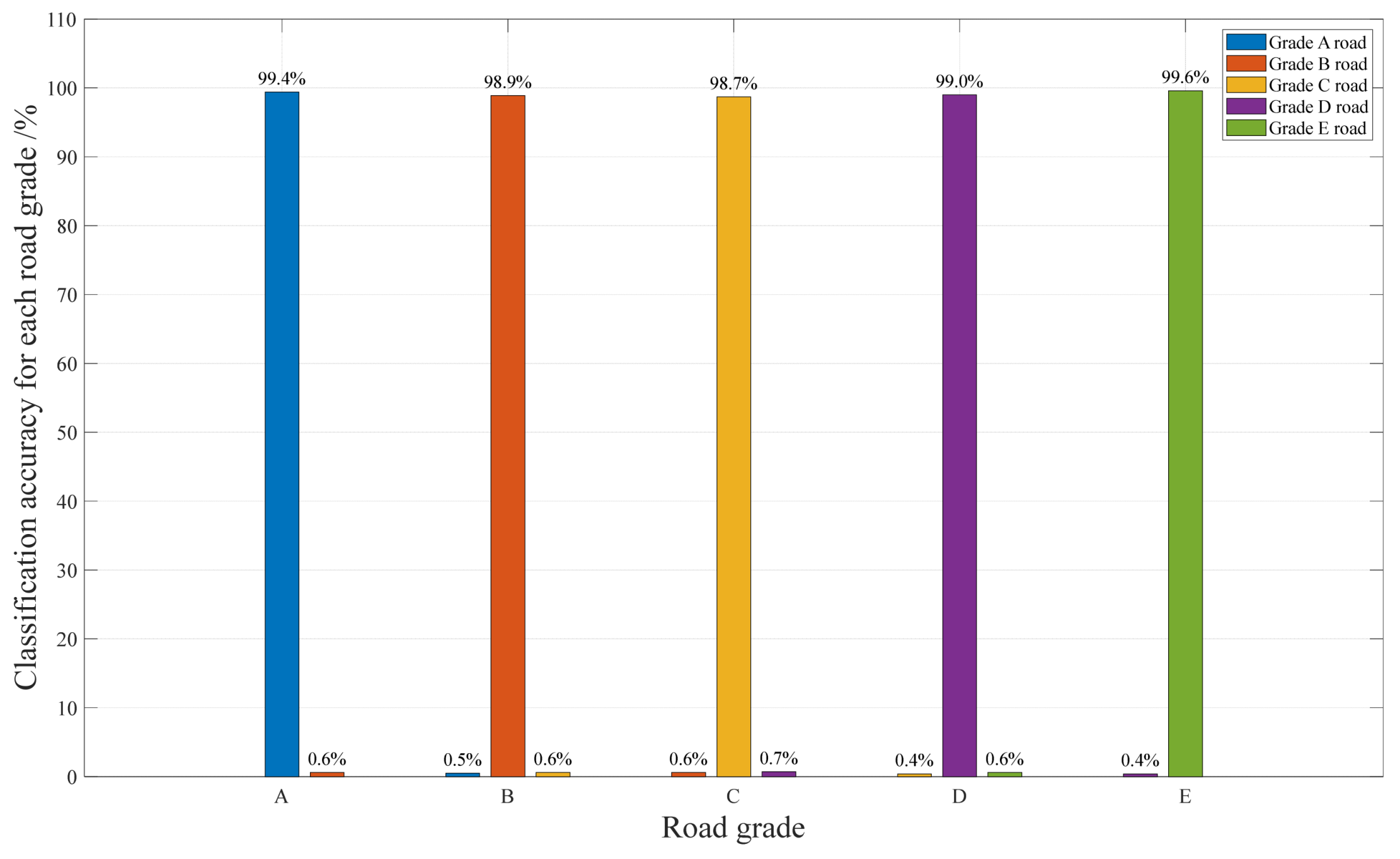
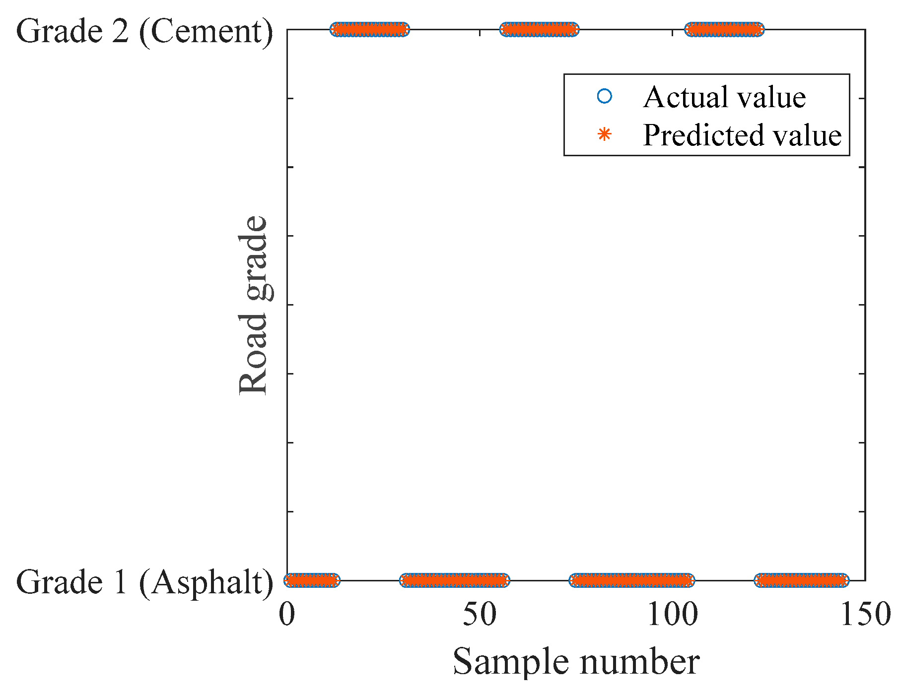
3.5. Real Road Roughness Classification

The simulation experiments in Section 3.4 have demonstrated that the KNN recognition road classification accuracy is extremely high (above 99.12%) when vehicle speed is consistently considered as a classification feature and any one of the proposed unsprung vertical vibration acceleration features (MAE, ASD, PAV, and RMS) is included together with the vehicle speed feature. To verify this conclusion, the actual collected road spectrum data will be classified in this section.
The vehicle was driven on four different test road sections (Figure 22) at constant speeds of 6, 8, and 10 km/h on the same road surface. The vertical acceleration response of the vehicle’s front wheel (single wheel) was collected. To enhance the efficiency of classification, the collected acceleration response data were used directly for road surface classification without any preprocessing, relying solely on the raw vertical acceleration response data.
Although section 1 and section 2 represent different road segments, they are both constructed with asphalt as the base material. Similarly, section 3 and section 4 are both constructed with concrete. To demonstrate that section 1 and section 2 belong to the same road surface category, and section 3 and section 4 belong to another, an equal number of unsprung vertical acceleration data points were extracted from the four road sections at a vehicle speed of 10 km/h. Time-domain and frequency-domain plots were constructed for the four test road sections, as shown in Figure 23 and Figure 24, respectively.
From Figure 23 and Figure 24, it can be seen that the road roughness grades of road sections 1 and 2 are almost the same, which is the same for road sections 3 and 4. Therefore, these four road sections are essentially two different roads. KNN is used to classify and recognize the measured road roughness, and the average absolute value of the original data of under-spring vibration acceleration and the corresponding speed are selected as the characteristics for road roughness recognition. A small number of data points with the same speed under the above four different test sections are randomly sorted to form a new recognition matrix array. The recognition effect is shown in Figure 25.
As shown in Figure 25, the speed-adaptive KNN classifier accurately distinguishes the road surfaces into two categories, achieving a classification accuracy of 100%, which is consistent with the results demonstrated in Figure 23 and Figure 24.
The above experiments of classifying four measured road surfaces verify the classification performance of the speed adaptive classifier, and the results show that the designed speed adaptive classifier accurately classifies the current road under different speed conditions.

4. Conclusions

This paper proposes a classification method for road roughness recognition, using a two-degree-of-freedom vehicle vertical vibration model based on simulation and real-vehicle tests. The strong correlation between the unsprung mass vertical vibration response of the vehicle and road roughness is revealed. Simulation tests indicate that the R2 of their correlation is 0.997 in both time and frequency domains. Real vehicle tests show that when the vehicle is traveling on the same road surface, the unsprung vertical vibration displacements of the left and right wheels closely correspond to the road beneath them. Both simulation and real-vehicle tests show that it is feasible to use the unsprung mass vertical vibration response to recognize road roughness. On this basis, this paper designs a vehicle speed adaptive road roughness classifier, and compares the classification effects of different classifiers based on the unsprung vibration response only, combined with the vehicle speed information, through simulation and actual sample data, and improves the accuracy by about 20% compared with the pavement classifier that does not take the speed information into account (minimum: 98.88%, average: 99.615%), which proves its high accuracy and robustness. This study can provide accurate road excitation for adaptive real-time control of semi-active or active vehicle suspensions, which is of great significance in guiding the optimal design of suspension systems.
Although the proposed method performs well in road roughness recognition and classification, there is still much room for expansion in future research, and future work will consider the effects of different driving conditions (steering, acceleration, braking, etc.) on road roughness recognition and classification.

Author Contributions

Methodology, Z.C., J.X. and S.Y.; software, J.X., Z.C. and S.Y.; validation, J.X. and Z.C.; investigation, J.X., Z.C., S.Y. and J.L.; resources, Z.C.; writing—original draft preparation, J.X. and Z.C.; writing—review and editing, J.X., Z.C., S.L., S.Y. and J.L.; supervision, Z.C. and S.L.; and project administration, Z.C. All authors have read and agreed to the published version of the manuscript.

Funding

This research was funded by the China Postdoctoral Science Foundation (grant number: 2023T160780), the Postgraduate Research & Practice Innovation Program of Jiangsu Province (grant number: SJCX24_0403) and the National Natural Science Foundation of China (grant number: 52105063).

Institutional Review Board Statement

Not applicable.

Data Availability Statement

The data presented in this study are available on request from the corresponding author or first author.

Acknowledgments

We thank the anonymous reviewers for providing critical comments and suggestions that improved the manuscript.

Conflicts of Interest

The authors declare no conflicts of interest.

References

  1. Xiao, W.; Zhou, Y.; FU, Y.; Zhang, M. Analysis of the Influence of Soil on the Maneuverability of Military Off-road Vehicles. Acta Armamentarii 2024, 45, 288–298. [Google Scholar]
  2. Franceschetti, B.; Rondelli, V.; Capacci, E. Lateral stability performance of articulated narrow-track tractors. Agronomy 2021, 11, 2512. [Google Scholar] [CrossRef]
  3. Sun, W.; Li, C.; Wang, J. Research on Ride Comfort of an Off-road Vehicle with Compound Suspension. Automot. Eng. 2022, 44, 105–114+122. [Google Scholar]
  4. Islam, F.; Nabi, M.; Ball, J. Off-road detection analysis for autonomous ground vehicles: A review. Sensors 2022, 22, 8463. [Google Scholar] [CrossRef]
  5. Yuan, Y.; Yang, H.; Ding, L. Experimental Study and Modeling Considering the Influence of Wheel Load for Planetary Exploration Rovers. J. Mech. Eng. 2024, 60, 263–271. [Google Scholar]
  6. Wu, C.; Wen, L.; Chen, Z. Minimum-jerk velocity planning and control for CVT tractor velocity regulation. Trans. Chin. Soc. Agric. Eng. 2023, 39, 28–35. [Google Scholar]
  7. Chen, Z. Research on System Dynamics Analysis and Continuously Variable Speed of Tractor; Nanjing Agricultural University: Nanjing, China, 2020. [Google Scholar]
  8. Zheng, E.; Fan, Y.; Zhu, R. Prediction of the vibration characteristics for wheeled tractor with suspended driver seat including air spring and MR damper. J. Mech. Sci. Technol. 2016, 30, 4143–4156. [Google Scholar] [CrossRef]
  9. Wan, H.; Ou, Y.; Guan, X. Review of the perception technologies for unmanned agricultural machinery operating environment. Trans. Chin. Soc. Agric. Eng. (Trans. CSAE) 2024, 40, 1–18. [Google Scholar] [CrossRef]
  10. Li, Y.; Zhu, Z.; Zheng, L. Multi-objective control and optimization of active energy-regenerative suspension based on road recognition. J. Traffic Transp. Eng. 2021, 21, 129–137. [Google Scholar]
  11. Yang, Z.; Shi, C.; Zheng, Y. A study on a vehicle semi-active suspension control system based on road elevation identification. PLoS ONE 2022, 17, e0269406. [Google Scholar] [CrossRef]
  12. Zhang, Z. Power Function Model Identification of Road Statistical Characteristics Based on International Roughness Index and Vehicle Vibration Response; Jilin University: Changchun, China, 2019. [Google Scholar]
  13. Duan, H.; Shi, F.; Zhao, Y. Research and practice of road surface profile measurement. J. Vib. Shock 2011, 30, 155–160. [Google Scholar]
  14. Zhao, X.; Li, J.; Yue, D. The road roughness acquisition test and analysis of three-dimensional lidar orchard pavement. J. Huazhong Agric. Univ. 2022, 41, 227–236. [Google Scholar]
  15. Chen, H.; Shao, Y. Measurement method of pavement surface spectrum with multi-sensor coupling based on inertial benchmark. J. Jilin Univ. (Eng. Technol. Ed.) 2023, 53, 2254–2262. [Google Scholar]
  16. Fares, A.; Zayed, T. Industry-and academic-based trends in pavement roughness inspection technologies over the past five decades: A critical review. Remote Sens. 2023, 15, 2941. [Google Scholar] [CrossRef]
  17. Berti, M.; Corsini, A.; Daehne, A. Comparative analysis of surface roughness algorithms for the identification of active landslides. Geomorphology 2013, 182, 1–18. [Google Scholar] [CrossRef]
  18. Gorges, C.; Öztürk, K.; Liebich, R. Impact detection using a machine learning approach and experimental road roughness classification. Mech. Syst. Signal Process. 2019, 117, 738–756. [Google Scholar] [CrossRef]
  19. Zhang, Q.; Hou, J.; Hu, X. Vehicle parameter identification and road roughness estimation using vehicle responses measured in field tests. Measurement 2022, 199, 111348. [Google Scholar] [CrossRef]
  20. Ngwangwa, H.; Heyns, P.; Labuschagne, F. Reconstruction of road defects and road roughness classification using vehicle responses with artificial neural networks simulation. J. Terramech. 2010, 47, 97–111. [Google Scholar] [CrossRef]
  21. Li, Z.; Zhang, W.; Liu, Q. Study on road roughness recognition based on analysis of wheel vertical dynamic load. Chin. J. Sci. Instrum. 2006, 2132–2133. [Google Scholar] [CrossRef]
  22. Li, J.; Guo, W.; Gu, S. Road Roughness Identification Based on NARX Neural Network. Automot. Eng. 2019, 41, 807–814. [Google Scholar]
  23. Liu, L.; Zhang, Z.; Lu, H. Road Roughness Identification Based on Augmented Kalman Filtering with Consideration of Vehicle Acceleration. Automot. Eng. 2022, 44, 247–255+297. [Google Scholar]
  24. Li, S.; Li, J.; Feng, G. Road roughness recognition based on GA-LSTM adaptive Kalman filtering. J. Vib. Shock 2024, 43, 121–130. [Google Scholar]
  25. Chen, K.; Shi, S.; Cheng, S. Research on Road Roughness Recognition Algorithm Based on ReliefF-RBF. Chin. J. Automot. Eng. 2024, 14, 49–59. [Google Scholar]
  26. Rahman, M.; Rideout, G. Using the lead vehicle as preview sensor in convoy vehicle active suspension control. Veh. Syst. Dyn. 2012, 50, 1923–1948. [Google Scholar] [CrossRef]
  27. Fergani, S.; Menhour, L.; Sename, O. A new LPV/H∞ semi-active suspension control strategy with performance adaptation to roll behavior based on non linear algebraic road profile estimation. In Proceedings of the 52nd IEEE Conference on Decision and Control, Florence, Italy, 10 December 2013. [Google Scholar]
  28. Imine, H.; Delanne, Y.; M’sirdi, N. Road profile input estimation in vehicle dynamics simulation. Veh. Syst. Dyn. 2006, 44, 285–303. [Google Scholar] [CrossRef]
  29. Doumiati, M.; Martinez, J.; Sename, O. Road profile estimation using an adaptive Youla–Kučera parametric observer: Comparison to real profilers. Control Eng. Pract. 2017, 61, 270–278. [Google Scholar] [CrossRef]
  30. Alatoom, Y.; Al-Suleiman, T. Development of pavement roughness models using Artificial Neural Network (ANN). Int. J. Pavement Eng. 2022, 23, 4622–4637. [Google Scholar] [CrossRef]
  31. Lugner, P.; Ploechl, M.; Imine, H. Road Profile Inputs for Evaluation of The Loads on The Wheels. Tyre Models for Vehicle Dynamics Analysis. In Proceedings of the 3rd International Colloquium on Tyre Models for Vehicle Dynamics Analysis (Tmvda), Vienna, Austria, 29–31 August 2004; Volume 2005, p. 43. [Google Scholar]
  32. Qin, Y. Study on Load Control System of Combined Harvester; Jiangsu University: Zhenjiang, China, 2012. [Google Scholar]
  33. Yin, J.; Chen, X.; Wu, L. Simulation Method of Road Excitation in Time Domain Using Filtered White Noise and Dynamic Analysis of Suspension. J. Tongji Univ. (Nat. Sci.) 2017, 45, 398–407. [Google Scholar]
  34. Shi, X.; Jiang, X.; Zhao, J.; Zhao, P.; Zeng, J. Seven Degrees of Freedom Vehicle Response Characteristic under Four Wheel Random Pavement Excitation. Sci. Technol. Eng. 2018, 18, 71–78. [Google Scholar]
  35. Chen, M.; Long, H.Y.; Ju, L.Y.; Li, Y.G. Stochastic road roughness modeling and simulation in time domain. Mech. Eng. Autom. 2017, 2, 40–41. [Google Scholar]
  36. ISO 8608:2016; Mechanical Vibration—Road Surface Profiles—Reporting of Measured Data. International Organization for Standardization: Geneva, Switzerland, 2016.
  37. Wang, J.; Li, P.; Han, Y. Road roughness measurement based on multi—Sensor data comprehension. Eng. J. Wuhan Univ. 2012, 45, 361–365. [Google Scholar]
  38. Wang, X.; Cheng, Z.; Ma, L. Road Recognition Based on Vehicle Vibration Signal and Comfortable Speed Strategy Formulation Using ISA Algorithm. Sensors 2022, 22, 6682. [Google Scholar] [CrossRef]
  39. Shen, Z.; Peng, Y.; Shu, N. A Road Damage Identification Method Based on Scale-span Image and SVM. Geomat. Inf. Sci. Wuhan Univ. 2013, 38, 993–997. [Google Scholar]
  40. Zhen, J.; Zhang, J.; Cao, D.; Wu, Y. Intelligent Roughness Detection of Asphalt Pavements by the kNN Method. J. South China Univ. Technol. (Nat. Sci. Ed.) 2022, 50, 50–56. [Google Scholar]
  41. Yu, T.; Pei, L.; Li, W.; Hu, Y. Pavement condition index prediction based on random forest algorithm. J. Road Transp. Res. Development. 2021, 38, 16–23. [Google Scholar] [CrossRef]
  42. Gu, S. Research on Neural Network Method for Pavement Roughness Recognition Based on Vehicle Response Neural Network Approach for Pavement Roughness Recognition Based on Vehicle Response; Jilin University: Changchun, China, 2018. [Google Scholar]
  43. Qin, Y.; Dong, M.; Zhao, F. Road Profile Classification for Vehicle Semi-Active Suspension System Based on Adaptive Neuro-Fuzzy Inference System. In Proceedings of the 2015 54th IEEE Conference on Decision and Control (CDC), Osaka, Japan, 15–18 December 2015; IEEE: Piscataway NJ, USA, 2015; pp. 1533–1538. [Google Scholar]
  44. Liang, G.; Zhao, T.; Wang, Y.; Wei, Y. Road Unevenness Identification Based on LSTM Network. Automot. Eng. 2021, 43, 509–517+628. [Google Scholar]
Figure 1. 2-DOF quarter-vehicle linear model.
Machines 13 00391 g001
Figure 2. Schematic of the sensor installation position.
Machines 13 00391 g002
Figure 3. Acceleration signal acquisition and process procedure.
Machines 13 00391 g003
Figure 4. Signal consistency verification procedure.
Machines 13 00391 g004
Figure 5. Time-domain comparison between Class-C road profile and unsprung mass vibration displacement.
Machines 13 00391 g005
Figure 6. Correlation analysis demonstrating the relationship between the Class-C road profile and the unsprung mass vibration displacement.
Machines 13 00391 g006
Figure 7. Frequency-domain correlation analysis demonstrating the relationship between the Class-C road profile and the unsprung mass vibration displacement.
Machines 13 00391 g007
Figure 8. Unsprung vertical vibration displacement of the left and right wheels at different speeds. (a) left wheel; (b) right wheel.
Machines 13 00391 g008
Figure 9. Frequency domain comparison of unsprung vibration displacement of the left and right wheels at different speeds.
Machines 13 00391 g009
Figure 10. SVM-based road roughness classification and recognition (without incorporating vehicle speed feature).
Machines 13 00391 g010
Figure 11. KNN-based road roughness classification and recognition (without incorporating the vehicle speed feature).
Machines 13 00391 g011
Figure 12. Random Forest-based road roughness classification and recognition (without incorporating vehicle speed feature).
Machines 13 00391 g012
Figure 13. RBF neural network-based road roughness classification and recognition (without incorporating vehicle speed feature).
Machines 13 00391 g013
Figure 14. SVM-based road roughness classification and recognition (incorporating vehicle speed feature).
Machines 13 00391 g014
Figure 15. KNN-based road roughness classification and recognition (incorporating vehicle speed feature).
Machines 13 00391 g015
Figure 16. Random Forest-based road roughness classification and recognition (incorporating vehicle speed feature).
Machines 13 00391 g016
Figure 17. RBF Neural Network-based road roughness classification and recognition (incorporating vehicle speed feature).
Machines 13 00391 g017
Figure 18. KNN-based road roughness classification and recognition (considering only vehicle speed and mean absolute value).
Machines 13 00391 g018
Figure 19. KNN-based road surface classification and recognition (considering only vehicle speed and absolute standard deviation).
Machines 13 00391 g019
Figure 20. KNN-based road roughness classification and recognition (considering only vehicle speed and peak absolute value).
Machines 13 00391 g020
Figure 21. KNN-based road roughness classification and recognition (considering only vehicle speed and root mean square value.
Machines 13 00391 g021
Figure 22. Test road sections. (a) section 1; (b) section 2; (c) section 3; (d) section 4.
Machines 13 00391 g022
Figure 23. Time-domain comparison of unsprung acceleration across four road segments at a speed of 10 km/h. (a) the whole sample; (b) the partial sample.
Machines 13 00391 g023
Figure 24. Frequency-domain comparison of unsprung vibration acceleration across four road segments at a speed of 10 km/h. (a) The whole sample; (b) the partial sample.
Machines 13 00391 g024
Figure 25. Classification accuracy of measured road surfaces using the KNN algorithm.
Machines 13 00391 g025
Table 1. Parameters for a quarter-vehicle model.
ParameterValue
Sprung mass m1133 kg
Unsprung mass m225 kg
Suspension stiffness Kc13,000 N/m
Suspension damping coefficient Cc2403.8 N·s/m
Tire stiffness Kt178,950 N/m
Table 2. Values of G q ( n 0 ) under different road grades.
Road Grade G q ( n 0 ) ·10−6 (m3)
Lower LimitGeometric MeanUpper Limit
A81632
B3264128
C128256512
D51210242048
E204840968192
F819216,38432,768
G32,76865,536131,072
H131,072262,144524,288
Table 3. Technical specifications of the triaxial acceleration sensor.
ParameterValue
Operating Voltage
Measurement Range
9–57 V
±16 g
Measurement Frequency266,667 Hz
Operating Temperature−40–85 °C
Communication InterfaceEthernet
Table 4. Definition of road database for different speed conditions.
Road GradesVehicle Speed (km/h)Simulation Duration
A5,10,15,20,25,30,35,40,45,50,55,601000 s for each speed
B5,10,15,20,25,30,35,40,45,50,55,601000 s for each speed
C5,10,15,20,25,30,35,40,45,50,55,601000 s for each speed
D5,10,15,20,25,30,35,40,45,50,55,601000 s for each speed
E5,10,15,20,25,30,35,40,45,50,55,601000 s for each speed
Table 5. Classification accuracy of different classifiers for road roughness recognition (without incorporating vehicle speed feature).
ClassifierClassification Accuracy
SVM
KNN
78.41%
74.92%
RF74.32%
RBF73.18%
Table 6. Classification accuracy of different classifiers for road roughness recognition (incorporating vehicle speed feature).
ClassifierClassification Accuracy
SVM
KNN
99.94%
100%
RF99.62%
RBF98.88%
Table 7. Classification accuracy of KNN with different feature selections.
Feature SelectionClassification Accuracy
Vehicle Speed, Mean Absolute Value
Vehicle Speed, Absolute Standard Deviation
100%
100%
Vehicle Speed, Peak Absolute Value99.12%
Vehicle Speed, Root Mean Square Value100%
Disclaimer/Publisher’s Note: The statements, opinions and data contained in all publications are solely those of the individual author(s) and contributor(s) and not of MDPI and/or the editor(s). MDPI and/or the editor(s) disclaim responsibility for any injury to people or property resulting from any ideas, methods, instructions or products referred to in the content.

