Article

Output Feedback Control of Dual-Valve Electro-Hydraulic Valve Based on Cascade Structure Extended State Observer Systems with Disturbance Compensation

1
State Key Laboratory of Crane Technology, Yanshan University, Qinhuangdao 066004, China
2
School of Mechanical Engineering, Yanshan University, Qinhuangdao 066004, China
3
Hebei Provincial Key Laboratory of Heavy Machinery Fluid Power Transmission and Control, Yanshan University, Qinhuangdao 066004, China
4
Beijing Sany Intelligent Manufacturing Technology Co., Ltd., Beijing 100005, China
5
Department of Applied Sciences, Northumbria University, Newcastle NE1 8ST, UK
*
Author to whom correspondence should be addressed.
Machines 2025, 13(5), 392; https://doi.org/10.3390/machines13050392
Submission received: 25 March 2025 / Revised: 6 May 2025 / Accepted: 7 May 2025 / Published: 8 May 2025
(This article belongs to the Section Automation and Control Systems)

Abstract

In the development trend of intelligent and high-performance construction machinery, the dual-spool electro-hydraulic valve, as a new-generation core control element, directly affects the operation accuracy and energy-efficiency level of construction machinery. The standard linear extended state observer (LESO) produces relatively serious peaks as the system order increases, which leads to the degradation of the observer’s performance and affects the controller’s accuracy. To solve this problem, this paper innovatively proposes an output feedback control strategy for a cascaded structure observer for the dual-spool electro-hydraulic valve. This paper designs an output feedback controller based on the cascaded structure observer. The uniform exponential stability (USE) criterion ensures that the tracking error of the observer for the system state is bounded. The expected load pressure is constructed based on the expected trajectory to replace the actual load pressure, avoiding the influence of the nonlinear coupling between the load pressure and the input signal on the control system. Finally, a stable output feedback controller is obtained based on the backstepping control method and Hurwitz polynomial stability analysis. This study first applies the cascaded structure observer to the field of dual-spool electro-hydraulic valve control, providing a new theoretical framework and technical path for the high-precision control of the hydraulic system of construction machinery. Theoretical analysis shows that compared with the standard LESO, the cascaded structure observer can significantly reduce the online computational burden and effectively suppress the peak phenomenon, providing stronger estimation ability. Finally, a large number of simulation examples verify the effectiveness and superiority of the output feedback controller based on the cascaded structure observer. In all four test scenarios, the average tracking error of C1 (the output feedback controller designed based on the cascaded structure linear extended state observer) is about 5.1%, the average tracking error of C2 (the output feedback controller designed based on the standard structure linear extended state observer) is about 7.8%, and the average tracking error of C3 (the high-gain PID controller) is about 19.2%. The average control accuracy of the designed C1 controller is improved by 2.7% and 14.1% compared with C2 and C3, respectively. In terms of the estimation of external disturbances, the average error of C1 is 14% and the average error of C2 is 29.6%. The estimation accuracy of the former is improved by 15.6% compared with the latter.

1. Introduction

There are complex and nonlinear characteristics in hydraulic valve control systems, such as the compressibility of oil, nonlinear friction, and component wear, which makes it difficult for traditional linear PID control technology to meet modern engineering needs [1]. Therefore, high-performance and reliable control strategies have always been a hot topic in the field of hydraulic transmission research.
Over years, many nonlinear control methods for electro-hydraulic control systems have appeared. For example, Guichao Yang et al. [2] used adaptive robust control technology on hydraulic servo actuators and achieved good position tracking and system parameter estimation. Weichao Sun et al. [3] used adaptive robust control technology and suppressed vibration in vehicle active suspensions. A Mohanty and B. Yao [4] used indirect adaptive robust control (IARC) technology and improved robotic arm trajectory tracking accuracy. References [5,6] used adaptive backstepping sliding film control and improved electro-hydraulic position servo system control accuracy. Yang Lin et al. [7] proposed a robust discrete-time sliding mode controller (DT-SMC) for the EHA system, which accurately simulated and compensated the system’s friction. Q. Guo et al. [8] presented a saturation adaptive control method which handled control saturation in a two-degree-of-freedom robotic arm motion system and achieved satisfactory control performance.
However, the above control methods heavily rely on full-state feedback. Due to cost and structural limitations, many hydraulic transmission systems do not have the conditions to achieve full state observers. Reference [9] proposed using low-pass filters to process the research object’s position information for obtaining velocity and acceleration information. However, the hysteresis effect from filtering and the introduction of other noise may lead to more serious system instability, reducing the controlled object’s control accuracy.
The extended state observer can estimate the immeasurable states in the system and estimate the parameter uncertainty and external disturbances in the system as concentrated disturbances, weakening the adverse effects of uncertainty factors on the system. In reference [10], researcher Han Jingqing proposed for the first time the active disturbance rejection control (ADRC) method based on an extended state observer. This control method does not require strict and precise system model parameters, can achieve corresponding control results by adjusting parameters such as feedback gain and observer bandwidth, and has achieved success in practical applications. References [9,11] all adopt automatic disturbance rejection control technology to achieve precise control of valve-controlled cylinders. In reference [12], L Zhou et al. designed a non-integral chain DCMSS control method for servo motors based on a generalized extended state observer (GESO) and verified it in simulation examples. In [13], Wonhee Kim et al. designed a feedback control method with a high-gain observer and a passive controller, effectively improving the position-tracking performance of the electro-hydraulic system.
However, the self-disturbance rejection control technology is limited by the performance of the extended state observer, and in some cases, the control effect is not satisfactory. Especially, the peak phenomenon that occurs during the transient period of the observer can easily induce instability in the feedback control system [14]. In addition, as the order of the system increases, in order to ensure the tracking effect of the high-dimensional state of the system, the observer gain needs to be increased to an exaggerated level [15] which will increase the sensitivity of the system controller to input noise and cause a substantial decline in its stability.
To reduce the impact of the peak phenomenon on controller performance, many scholars have conducted research. In reference [16], Y Huang et al. proposed an event-triggering strategy based on output feedback, which ensures real-time boundedness of observation errors by designing reasonable triggering conditions. In [17], M S. Chong et al. proposed a hybrid estimation scheme for parameters and states based on multi-state observers. By switching different observers while the excitation conditions persist, the estimation errors of parameters and states converge and are bounded. In [18], Ricardo G. Sanfelice and Laurent Praly proposed an adaptive adjustment algorithm for observer gain, suppressing the problem of an abnormal increase in the observation gain of the system under strong noise or transient conditions. The improved extended state observer proposed in the above research can achieve better estimation performance compared to the standard extended state observer, but it is more complex in structure and increases the difficulty of application in practical engineering.
In reference [19], D. Astolfi and L. Marconi proposed a new type of observer which cascades adjacent system channels (in a control system, the pathways of each transmission link are called system channels) in a structure. The system state is transmitted through the previous channel to the next level, thus avoiding the problem of the gain of the standard observer falling into an “exponential explosion”. Maopeng Ran et al. proposed a new type of extended state observer based on the cascaded first-order extended state observer [20]. In high-order systems, this observer can limit the peak value of internal variables by adjusting a small number of parameters. More importantly, in terms of structure, this linear extended state observer designed based on a cascaded structure is as concise as the standard extended state observer.
Inspired by reference [19,20], this paper designs a cascaded structure-based extended state observer and output feedback controller for a dual-spool electro-hydraulic valve control system. Through a large number of simulation examples, it is verified that the proposed controller based on the new observer design has a better performance compared to the standard structure, making it possible to apply it in hydraulic transmission systems.
The main contributions of this paper are summarized below: (1) the proposed output feedback controller obtains unknown system states and external disturbances by constructing a cascaded extended state observer, effectively avoiding the peak phenomenon when the standard extended state observer is applied to high-order systems; (2) in response to the nonlinear coupling phenomenon between the driving pressure and input voltage of the dual-valve core electro-hydraulic valve, the expected trajectory of the valve core is used to obtain the expected driving pressure of the valve core to release the coupling relationship and effectively reduce the online calculation burden of the controller.
The rest of this paper includes the following: problem formulation can be seen in Section 2; the controller design procedure and its theoretical results are presented in Section 3; and the simulation results of four examples and the conclusion are accordingly observed from Section 4 and Section 5.

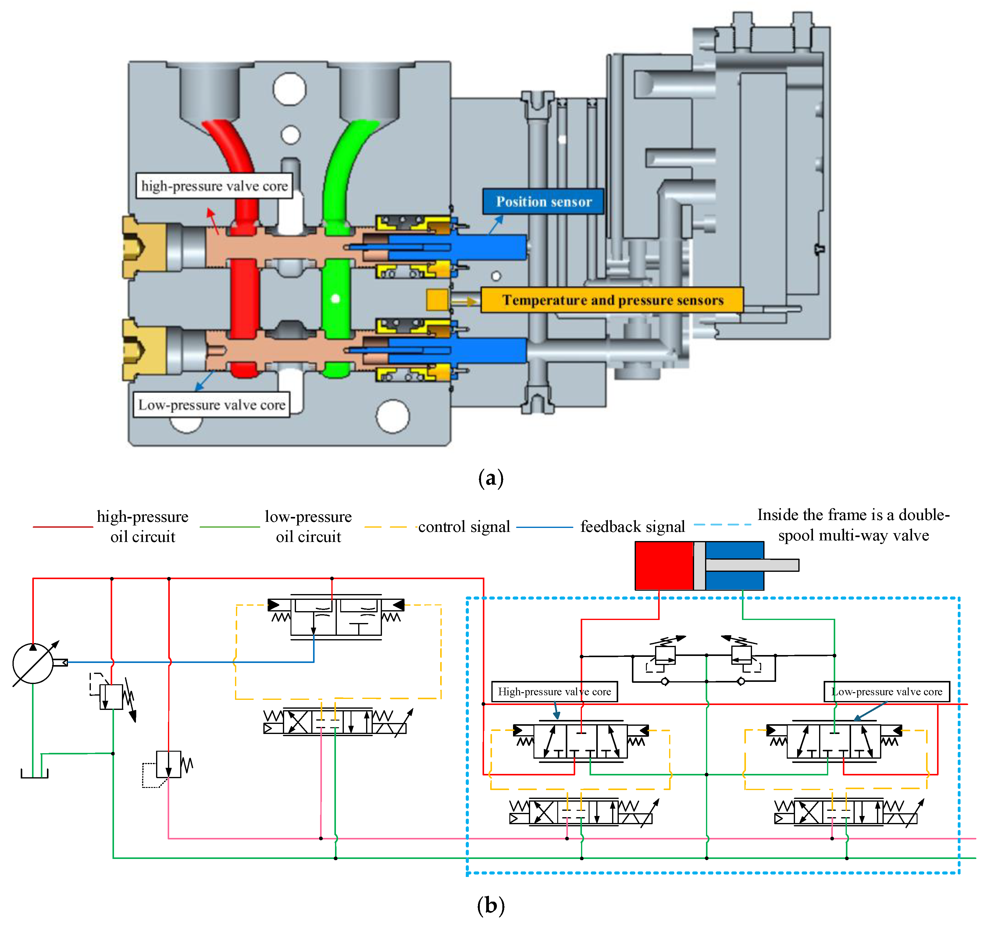
2. Problem Formulation

This paper focuses on the research of a cascaded structure expansion state observer based on a self-developed dual-spool electro-hydraulic valve, as shown in Figure 1.
As shown in Figure 1, the dual-valve core electro-hydraulic valve studied in this paper consists of two three-position four-way high-frequency response proportional pilot valves and two three-position three-way main valves. The pilot stage valve core integrates LVDT displacement sensors, which can achieve closed-loop control of the pilot valve displacement. The two main valve cores are the high-pressure valve core and the low-pressure valve core, respectively. The high-pressure valve core is used for oil inlet control and the low-pressure valve core is used for oil return control, thus achieving independent control of the load port. A displacement sensor is installed on the main valve core, and a temperature and pressure sensor is installed in the flow channel between the main valve core and the actuator to sense the oil temperature and load pressure.
Before establishing a nonlinear mathematical model of an electro-hydraulic servo system, this article defines the following parameters (Table 1).
The goal of the controller designed in this article is to achieve high-precision tracking of the expected trajectory of the main valve displacement when only obtaining the displacement and oil supply pressure of the dual-spool electro-hydraulic valve. The hydraulic system maintains a constant oil supply pressure of P s through the accumulator safety valve group, and the oil hydraulic force of P r in the oil tank is considered zero pressure.
The dynamic model of the main valve core can be described by the following equation:
m y ¨ = P 1 A 1 P 2 A 2 k y + d 1
where d 1 represents the modeling error including nonlinear friction and the concentrated disturbance caused by external disturbances, and y represents the spool displacement of the main valve.
The dynamic model of load force P L at both ends of the main valve core is given by the following equation:
V t 4 β e P ˙ L = Q L A y ˙ + d 2
Due to the dual-spool valve electro-hydraulic valve system depicted in Figure 1 using a high-frequency-response pilot valve as the control input for the main valve and based on the processing method in reference [9], this paper ignores the dynamic model of the pilot valve and considers it as a proportional relationship between the voltage and pilot valve opening, namely, x v = k v u , where the load flow rate Q L can be expressed as:
Q L = k v k q P s sign ( k v u ) P L u
where k q is the flow gain corresponding to the displacement of the pilot valve core, and s i g n ( · ) is the standard symbol function.
Define the state variable x = [ x 1 , x 2 , x 3 ] T = [ y , y ˙ , y ¨ ] T and write the state-space equation of the entire system as follows:
x ˙ 1 = x 2 x ˙ 2 = x 3 x ˙ 3 = h ( P L ) u + h 1 ( x 2 ) B m x 3 + d
where
h ( P L ) = 4 A k v k q β e m V t P s s i g n ( k v u ) P L h 1 ( x 2 ) = ( 4 A 2 β e m V t + k m ) x 2 d = 1 m d 1 4 A β e m V t d 2
Based on Equations (4) and (5), it can be observed that there is a coupling phenomenon between the controller voltage u and the load pressure P L . In subsequent stability analysis, if load pressure P L is not measurable then the proof of system stability will not be achieved. Therefore, it is necessary to further study the coupling relationship between voltage u and load pressure P L .
According to the method in [21], the expected trajectory is combined with the system power head model, then the expected load pressure signal can be synthesized:
x ¨ 1 d = A P L d m B m x ˙ 1 d k m x 1 d P L d = m A x ¨ 1 d + B A x ˙ 1 d + k A x 1 d
By replacing the actual load pressure with the expected load pressure P L d in Equation (6), the nonlinear coupling phenomenon between the controller output voltage and load pressure can be relieved. The system state equation can be rewritten as follows:
x ˙ 1 = x 2 x ˙ 2 = x 3 x ˙ 3 = h ( P L d ) u + h 1 ( x 2 ) B m x 3 + D ( t )
where
h ( P L ) = 4 A k v k q β e m V t P s s i g n ( k v u ) P L D ( t ) = 1 m d 1 4 A β e m V t d 2 + [ h ( P L ) h ( P L d ) ] u

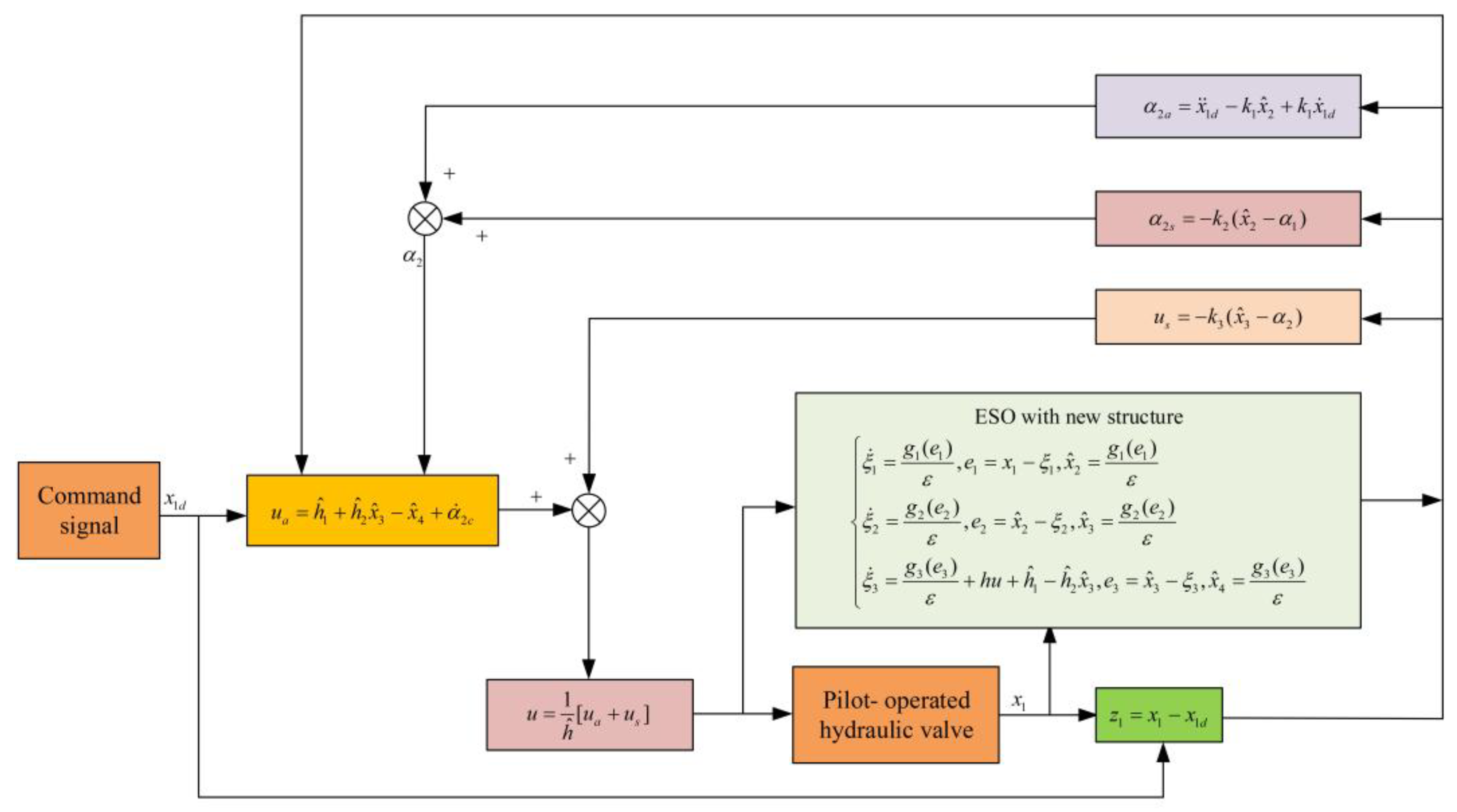
3. Cascade Observer and Output Feedback Controller Design

3.1. Preliminary Assumptions of Controller Design

It should be pointed out that the hydraulic system studied in the article is affected by factors such as oil temperature changes and component wear that are not considered during actual operation, which can lead to changes in system parameters such as B and β e . In order to simplify the control scheme, the nominal values of the above physical parameters will be used for subsequent design. The resulting parameter deviations can be considered and concentrated in the system modeling error D ( t ) .
In the following text, an output feedback control strategy will be discussed to overcome internal and external disturbances in the system so that the valve spool of the main valve follows any smooth expected trajectory as much as possible.
The following assumptions run through the entire paper:
Assumption 1.
P L  is much smaller than  P s , which ensures that function h ( P L ) is far away from 0.
Assumption 2.
When  u 0 , h ( P L )  is continuously differentiable. At u = 0 , the left and right derivatives of h ( P L ) exist and are bounded, thus ensuring that function h ( P L ) satisfies the Lipschitz condition with respect to P L in the domain of a function.
Assumption 3.
Function  h 1 ( x 2 )  satisfies the Lipschitz condition with respect to  x 2  in the domain of a function.
Assumption 4.
The disturbances  d 1 ( t )  and  d ˙ 2 ( t )  exist and are bounded by d 1 ( t ) δ 1 and d ˙ 2 ( t ) δ 2 .
For the convenience of writing, in the following text, this article will write D ( t ) as D ; dunction h ( P L )   h 1 ( x 2 ) as h   h 1 ; h ^ 1 for the function h 1 ( x ^ 2 ) containing observations; and h ˜ 1 = h 1 h ^ 1 .

3.2. Design of Extended State Observer with Cascade Structure

In this section, an ESO with a cascaded structure will be designed to estimate the unknown state of the system and the concentrated disturbances including modeling errors. The above observed and estimated values will be used to achieve real-time compensation for the controller.
Prior to this, the modeling error D in the state-space equation needs to be extended to an additional system state variable. The system variable x is extended to [ x 1 , x 2 , x 3 , x 4 ] T = [ y , y ˙ , y ¨ , D ] T , and g ( t ) is defined as the derivative of x 4 and satisfies the Lipschitz condition. Therefore, the original system state-space Equation (8) can be rewritten as follows:
x ˙ 1 = x 2 x ˙ 2 = x 3 x ˙ 3 = h u + h 1 B m x 3 + x 4 x ˙ 4 = g ( t )
Define x ^ as the estimated value of system state, where x ^ i is the estimated value of x i ( i = 1 , 2 , 3 , 4 ) and x ˜ = x x ^ = [ x ˜ 1 , x ˜ 2 , x ˜ 3 , x ˜ 4 ] is the state-estimated error. Based on the extended system model (10), LESO can be constructed as [20], which is as follows:
ξ ˙ 1 = g 1 ( e 1 ) ε , e 1 = x 1 ξ 1 , x ^ 2 = g 1 ( e 1 ) ε ξ ˙ 2 = g 2 ( e 2 ) ε , e 2 = x ^ 2 ξ 2 , x ^ 3 = g 2 ( e 2 ) ε ξ ˙ 3 = g 3 ( e 3 ) ε + h u + h ^ 1 B m x ^ 3 , e 3 = x ^ 3 ξ 3 , x ^ 4 = g 3 ( e 3 ) ε g i ( · ) = l i ·
where ξ = [ ξ 1 , ξ 2 , ξ 3 ] T R 3 is an internal variable of the system, ε < 1 is an adjustable positive parameter, and parameter L = [ l 1 , l 2 , l 3 ] is the gain of LESO, which is determined by making λ 3 + l 1 λ 2 + l 2 λ + l 3 the Hurwitz polynomial.
Compared with conventional LESO, the designed observer with a new structure has a channel output that is the input of the channel, meaning there is a connection relationship between adjacent channels. In addition, observer (11) can be seen as a cascade of three first-order extended state observers, effectively reducing the negative impact of high-gain coefficients of conventional observers on high-dimensional observation objects.

3.3. Convergence Analysis of the Observer

Before proving the convergence of observer (10), some conclusions about time-varying systems need to be cited.
Theorem 1.
The following time-variant system is defined [22]:
ζ ˙ ( t ) = ϖ ( t ) ζ ( t ) ,   t R +
where ϖ ( t ) c ( R + ) is a n-order matrix. System (11) is called consistent Exponential stability (USE).
Lemma 1.
For the following time-variant system:
ζ ˙ ( t ) = 1 ε ϖ ( t ) ζ ( t ) + δ ( t ) ,   t t 0 ,   t 0 R +
where ϖ ( t ) c ( R + ) is an n-order order matrix, δ ( t ) is the disturbance in the system, and its initial condition ζ ( t 0 ) belongs to a compact subset of R n .
Assume that the linear time-variant system ζ ˙ 0 ( t ) = ϖ ( t ) ζ 0 ( t ) satisfies the USE condition, and for some normal numbers δ and integer r that are independent of ε and satisfy δ ( t ) δ ε r , then for σ > 0 and T > 0 both ε 0 > 0 make the solution of system (20) satisfy ζ ( t ) σ ε r for ε ( 0 , ε 0 ) and t [ t 0 + T , ε 0 ) .
The following assumption is necessary to prove the convergence of the observer and is reasonable.
Assumption 5.
Function g i ( i = 1 , 2 , 3 )  is an n-order differentiable and there are constants independent of ε that satisfy inequalities 0 < r 1 r 1 and r j > 0 such that r 1 g i ( e i ) r 1 and g i ( j ) ( e i ) m j .
Define the following:
g i ( e i ) d g i ( e i ) d e i , g i ( j ) ( e i ) d j g i ( e i ) d e i j
Assumption 6.
The control input u and system state x are bounded.
Considering the uncertain nonlinear system (10) and the proposed observer (11), under the condition that the above assumptions 1–5 are satisfied and the observer is a compact subset of R n at the initial time, the following conclusions can be obtained: for σ > 0 and T > 0 both ε * > 0 make ε ( 0 , ε * ) satisfy the following equation:
x i ( t ) x ^ i ( t ) σ , 2 i 4 , t T
Proof. 
In this article, the convergence of observation errors will be achieved by sequentially converging each order of error. Because assuming 1–6 is satisfied, it is easy to obtain that each order state in the system is bounded and that each stage of observer (10) is a stable system. Therefore, the existence of x ^ 2 to x ^ 4 is guaranteed.
Define ethe following error vector:
η ˜ n = [ η 2 , , η n ] T , 2 n 4 η i = ε i 1 ( x i x ^ i ) , 2 i 4
For the convenience of subsequent proof, define the following:
H j = [ 0 , , 1 ] R 1 × j 1 , 3 j 4
Step 1: The derivative of η 2 can be represented by the following equation:
η ˙ 2 = ε x ˙ 2 x ^ ˙ 2 = ε x ˙ 2 ε x ^ ˙ 2 = 1 ε g 1 e 1 η 2 + ε x 3
note that the above equation belongs to the form of system (18), and it is known that x 2 and x 3 are bounded. Through Lemma 1, it is known that there exists ε 1 > 0 for σ > 0 , 0 < g 1 e 1 < r 1 , T > 0 , and T 1 0 , T to satisfy any η 2 t σ ε , which is equivalent to the case of i = 2 in (15).
Step 2: The derivative of η 3 can be represented by the following equation:
η ˙ 3 = ε 2 x ˙ 3 x ^ ˙ 3 = 1 ε g 1 e 1 g 2 ( e 2 ) η 2 1 ε g 2 ( e 2 ) η 3 + ε g 2 ( e 2 ) x 3 + ε 2 ( h u + h 1 h 2 x 3 + x 4 )
According to the definition of error vector η ˜ n , considering Equations (17) and (18), the derivative of η ˜ 3 can be written as follows:
η ˜ ˙ 3 = 1 ε ϕ 31 η ˜ 3 + ε ϕ 32 x 3 + ε 2 ϕ 33 h u + h 1 h 2 x 3 + x 4
where
ϕ 31 = g 1 e 1 0 g 1 e 1 g 2 e 2 g 2 e 2   ,   ϕ 32 = 1 g 2 e 2   ,   ϕ 33 = 0 1
It should be pointed out that ϕ 31 is reversible for t [ 0 , ) , and by defining ψ 3 = η ˜ 3 + ε 2 ϕ 31 1 ϕ 32 x 3 , the following equation can be easily obtained:
ψ ˙ 3 = 1 ε ϕ 31 ψ 3 + ε 2 d ( ϕ 31 1 ϕ 32 ) d t x 3 + ε 2 ( ϕ 31 1 ϕ 32 + ϕ 33 ) ( h u + h 1 h 2 x 3 + x 4 )
According to the results of Step 1, for t > Τ 1 the second and third items on the right side of Equation (22) are in the form of O ( ε 2 ). Combining Lemma 1, it can be confirmed that the derivative of ψ 3 is in the form of parameter m = 2 in system (15). Therefore, it can be concluded that for σ > 0 and T 2 ( T 1 , T ) there exists ε 2 ( 0 , ε 1 ] that satisfies ψ 3 t σ ε 2 for any ε 0 , ε 2 ,   t 1 T 2 , . On the other hand, η 3 can be written as follows:
η 3 = H 3 η ˜ 3 = H 3 ψ 3 ε 2 H 3 ϕ 31 1 ϕ 32 x 3 = H 3 ψ 3
where
H 3 ϕ 31 1 ϕ 32 = [ 0   1 ] 1 g 1 e 1 0 1 1 g 2 e 2 1 g 2 ( e 2 ) = 0
So it can be concluded that for σ > 0 , T 2 T 1 , T there exists a case where ε 2 ( 0 , ε 1 ] satisfies η 3 t σ ε 2 for any ε 0 , ε 1 ,   t T 2 , , which is equivalent to the case of i = 3 in (14).
Step 3: The derivative of η 4 can be represented by the following equation:
η ˙ 4 = ε 3 ( x ˙ 4 x ^ ˙ 4 ) = ε 3 g ( t ) + g 3 ( e 3 ) ( η ˙ 3 ) 1 ε g 3 ( e 3 ) η 4 + ε 2 g 3 ( e 3 ) [ h u + h ^ 1 B m x ^ 3 ] = ε 3 g ( t ) + g 3 ( e 3 ) ( η ˙ 3 ) 1 ε g 3 ( e 3 ) η 4 + ε 2 g 3 ( e 3 ) [ h u + ( h ^ 1 h 1 ) + B m ( x 3 x ^ 3 ) ] + ε 2 g 3 ( e 3 ) ( h 1 B m x 3 )
Since functions h 1 ( x 2 ) and h 2 ( x 2 ) satisfy the Lipschitz condition with respect to x 2 in the domain of a function, there exists a constant c1 that satisfies the following:
u u max   ,   h 1 h ^ 1 c 1 η 2  
η ˙ 4 ε 3 g ( t ) + g 3 ( e 3 ) ( η ˙ 3 ) 1 ε g 3 ( e 3 ) η 4 + ε 2 g 3 ( e 3 ) ( h u max + c 1 η 2 + B m ε 2 η 3 ) + ε 2 g 3 ( e 3 ) ( h 1 B m x 3 )
By assuming 4 and 6, it can be seen that the constraints imposed on g ( t ) , x 2 , and x 3 are independent of ε . Based on the boundedness of g ( t ) , x 2 , and x 3 , the above equations belong to the form of system (10). Therefore, through Lemma 2 it can be concluded that for σ > 0 , T 3 T 2 , T there exists a case where ε 3 ( 0 , ε 2 ] satisfies η 4 t σ ε 3 for any ε 0 , ε 3 ,   t T 3 , , which is equivalent to the case of i = 4 in (14). □
In summary, the estimation errors of each order system state of observer (10) are bounded and the observer parameters can be adjusted to minimize the observation error.

3.4. Design of Output Feedback Controller

Step 1: Define an error variable z 2 as follows:
z 2 = z ˙ 1 + k 1 z 1 = x 2 α 1
where z 1 = x 1 x 1 d ( t ) is the tracking error of the system output position, α 1 x ˙ 1 d k 1 z 1 is the virtual control rate of the system state x 2 , and z 2 represents the difference.
From Equation (23), it can be seen that due to the inclusion of unknown state x 2 , signal z 2 in the controller is not measurable. Therefore, z 2 needs to be divided into computable z 2 c and incomputable parts z 2 u . As a result, z 2 c is calculated by obtaining x ^ 2 through observer (13) and used for subsequent controller design, as shown below:
z 2 = z 2 c + z 2 u   ,   z 2 c = x ^ 2 α 1 , z 2 u = x ˜ 2
Based on Equations (10) and (27), the derivative of z 2 can be expressed as follows:
z ˙ 2 = x ˙ 2 α ˙ 1 = x 3 α ˙ 1
Based on the design concept of the backstepping method, x 3 is considered as the virtual control input of the system. Next, the control law α 2 will be designed to ensure the control performance of the system.
By defining z 3 = x 3 α 2 as the control error of the virtual control input and incorporating Equation (29), the following equation can be obtained:
z ˙ 2 = z 3 + α 2 x ¨ 1 d + k 1 x 2 k 1 x ˙ 1 d
Based on the state estimation obtained from observer (13), Equation (30) yields the virtual control rate α 2 as follows:
α 2 = α 2 a + α 2 s α 2 a = x ¨ 1 d k 1 x ^ 2 + k 1 x ˙ 1 d α 2 s = k 2 ( x ^ 2 α 1 )
where α 2 a is the model-based compensation term, α 2 s is the robust control term to achieve local stability of the system, and k 2 > 0 is the feedback gain.
By incorporating Equation (27) into Equation (31), z 2 can be reconstructed as follows:
z ˙ 2 = z 3 k 2 z 2 + k 1 + k 2 ε η 2
By differentiating z 3 from Equations (10) and (31), the following can be obtained:
z ˙ 3 = x ˙ 3 α ˙ 2 = h u + h 1 B m x 3 + x 4 α ˙ 2 c α ˙ 2 u
where α 2 c is the differentiable part in α 2 , and B is the non-differentiable part in α 2 , as shown below:
α ˙ 2 c = α 2 t + α 2 x 1 x ^ 2 + α 2 x ^ 2 x ^ ˙ 2 α ˙ 2 u = α 2 x 1 ( x 2 x ^ 2 ) = k 1 k 2 ( x 2 x ^ 2 )
The actual input u of the system can be synthesized through the following online state estimation values of the observer:
u = 1 h ^ [ u a + u s ] u a = h ^ 1 + B m x ^ 3 x ^ 4 + α ˙ 2 c u s = k 3 ( x ^ 3 α 2 )
where k 3 > 0 represents the feedback gain, u a represents the model compensation term obtained from the estimated state, and u s is the robust feedback term used to stabilize the system.
By incorporating Equation (31) into (29), z ˙ 3 can be reconstructed as follows:
z ˙ 3 = k 3 z 3 + k 3 x ˜ 3 + h ˜ 1 B m x ˜ 3 + k 1 k 2 x ˜ 2 + x ˜ 4 = k 3 z 3 + h ˜ 1 + k 1 k 2 ε η 2 + 1 ε 2 ( k 3 B m ) η 3 + η 4 ε 3
The overall framework of the controller is shown in Figure 2.

3.5. Proof of Convergence of Backstepping Controller

In this section, it will be proven that the backstepping controller mentioned above can make all error signals bounded when used in the system described in this article. Prior to this, additional explanations need to be provided for the observer’s error (10).
Define error vector η ˜ n = [ η 2 , , η n ] T , 2 n 4 .
According to Equations (17), (18), and (25), η ˙ 4 can be rewritten as follows:
η ˙ 4 = ε 3 ( x ˙ 4 x ^ ˙ 4 ) = 1 ε g 1 ( e 1 ) g 2 ( e 2 ) g 3 ( e 3 ) η 2 1 ε g 2 ( e 2 ) g 3 ( e 3 ) η 3 1 ε g 3 ( e 3 ) η 4 + ε g 2 ( e 2 ) g 3 ( e 3 ) x 3 + ε 3 g ( t ) + ε 2 g 3 ( e 3 ) ( x 4 + h u + h ^ 1 B m x ^ 3 )
According to the definition of error vector η ˜ n , combined with Equations (17), (19), and (37), the derivative of η ˜ 4 can be written as follows:
η ˜ ˙ 4 = 1 ε ϕ 41 η ˜ 4 + ε ϕ 42 x 3 + ε 3 ϕ 44 g ( t ) + ε 2 ϕ 43 ( x 4 + h u + h ^ 1 B m x ^ 3 ) + ε 2 ϕ 433 [ h ˜ 1 B m ( x 3 x ^ 3 ) ] = 1 ε ϕ 41 η ˜ 4 + ε ϕ 42 x 3 + ε 2 ϕ 433 [ h ˜ 1 B m ε 2 η 3 ] + ε 2 ϕ 43 ( x 4 + h u h ˜ 1 + h 1 + B m ε 2 η 3 B m x 3 ) + ε 3 ϕ 44 g ( t )
where
ϕ 41 = g 1 ( e 1 ) 0 0 g 1 ( e 1 ) g 2 ( e 2 ) g 2 ( e 2 ) 0 g 1 ( e 1 ) g 2 ( e 2 ) g 3 ( e 3 ) g 2 ( e 2 ) g 3 ( e 3 ) g 3 ( e 3 )   , ϕ 42 = 1 g 2 ( e 2 ) g 2 ( e 2 ) g 3 ( e 3 )   ,   ϕ 43 = 0 1 g 3 ( e 3 )   ,   ϕ 433 = 0 1 0   ,   ϕ 44 = 0 0 1
Since the parameter L = [ l 1 , l 2 , l 3 ] is determined by making λ 3 + l 1 λ 2 + l 2 λ + l 3 satisfy the Hurwitz polynomial, it is easy to obtain that ϕ 41 is the Hurwitz matrix, that is, there is a positive-definite symmetric matrix A satisfying the following:
ϕ 41 T A + A ϕ 41 = 2 E
where E is a third-order identity matrix.
The positive-definite matrix θ is defined as follows:
θ = 1 2 z 1 2 + 1 2 z 2 2 + 1 2 z 3 2 + 1 2 η ˜ 4 T A η ˜ 4
By differentiating Equation (41) and substituting it into Equations (32), (36), (38), and (40), the following can be obtained:
θ ˙ = z 1 z ˙ 1 + z 2 z ˙ 2 + z 3 z ˙ 3 + 1 2 η ˜ ˙ 4 T A η ˜ 4 + 1 2 η ˜ 4 T A η ˜ ˙ 4
θ ˙ = z 1 z ˙ 1 + z 2 z ˙ 2 + z 3 z ˙ 3 + 1 2 η ˜ ˙ 4 T A η ˜ 4 + 1 2 η ˜ 4 T A η ˜ ˙ 4 = z 3 [ k 3 z 3 + h ˜ 1 + k 1 k 2 ε η 2 + 1 ε 2 ( k 3 B m ) η 3 + η 4 ε 3 ] + z 2 ( z 3 k 2 z 2 + k 1 + k 2 ε η 2 ) + z 1 ( z 2 k 1 z 1 ) 1 ε η ˜ 4 2 + ε 2 η ˜ 4 T A ϕ 43 ( x 4 + h u h ˜ 1 + h 1 + B m ε 2 η 3 B m x 3 ) + ε 2 η ˜ 4 T A ϕ 433 [ h ˜ 1 B m ε 2 η 3 ] + ε 3 η ˜ 4 T A ε 3 ϕ 44 g ( t ) + ε η ˜ 4 T A ϕ 42 x 3
By assuming the definitions of 2, 3, and 6, there exists a normal number c 1 that satisfies the following:
h ˜ 1 c 1 η 2
Define a variable κ through the following:
κ = ε η ˜ 4 T A ϕ 42 x 3 + ε 3 η ˜ 4 T A ε 3 ϕ 44 g ( t ) + ε 2 η ˜ 4 T A ϕ 43 ( x 4 + h u + h 1 B m x 3 )
By assuming 2, 3, and 6, it can be obtained that the existence of a normal number κ max satisfies the inequality κ max κ .
Define a set of known constants through the following:
N 1 = k 1 + k 2 ε N 2 = k 1 k 2 ε + c 1 N 3 = 1 ε 2 ( k 3 B m ) N 4 = 1 ε 3 γ = ε 2 A ( ϕ 433 ϕ 43 ) c 1 + A ( ϕ 43 ϕ 433 ) B m
Considering (45) and (46), the following can be concluded:
θ ˙ k 1 z 1 2 k 2 z 2 2 k 3 z 3 2 + z 1 z 2 + z 2 z 3 ( 1 ε γ ) η ˜ 4 2 + N 1 z 2 η 2 + N 2 z 3 η 2 + N 3 z 3 η 3 + N 4 z 3 η 4 = ψ T Λ ψ + κ
where ψ = [ z 1 , z 2 , z 3 , η 2 , η 3 , η 4 ] T
Λ = k 1 1 2 0 0 0 0 1 2 k 2 1 2 N 1 2 0 0 0 1 2 k 3 N 2 2 N 3 2 N 4 2 0 N 1 2 N 2 2 1 ε γ 0 0 0 0 N 3 2 0 1 ε γ 0 0 0 N 4 2 0 0 1 ε γ
Select appropriate control parameters k 1 , k 2 , k 3 , and ε to make the matrix Λ a positive-definite matrix, and then obtain the following:
θ ˙ λ min ( Λ ) ( z 2 + η ˜ 4 2 ) + κ max λ min ( Λ ) ( z 2 + 1 λ max ( A ) η ˜ 4 T A η ˜ 4 ) + κ max τ θ + κ max
By integrating Equation (49), the following can be obtained:
θ ( t ) θ ( 0 ) e τ t + κ max τ 1 e τ t
Therefore, the tracking error of the system for the expected trajectory is bounded.

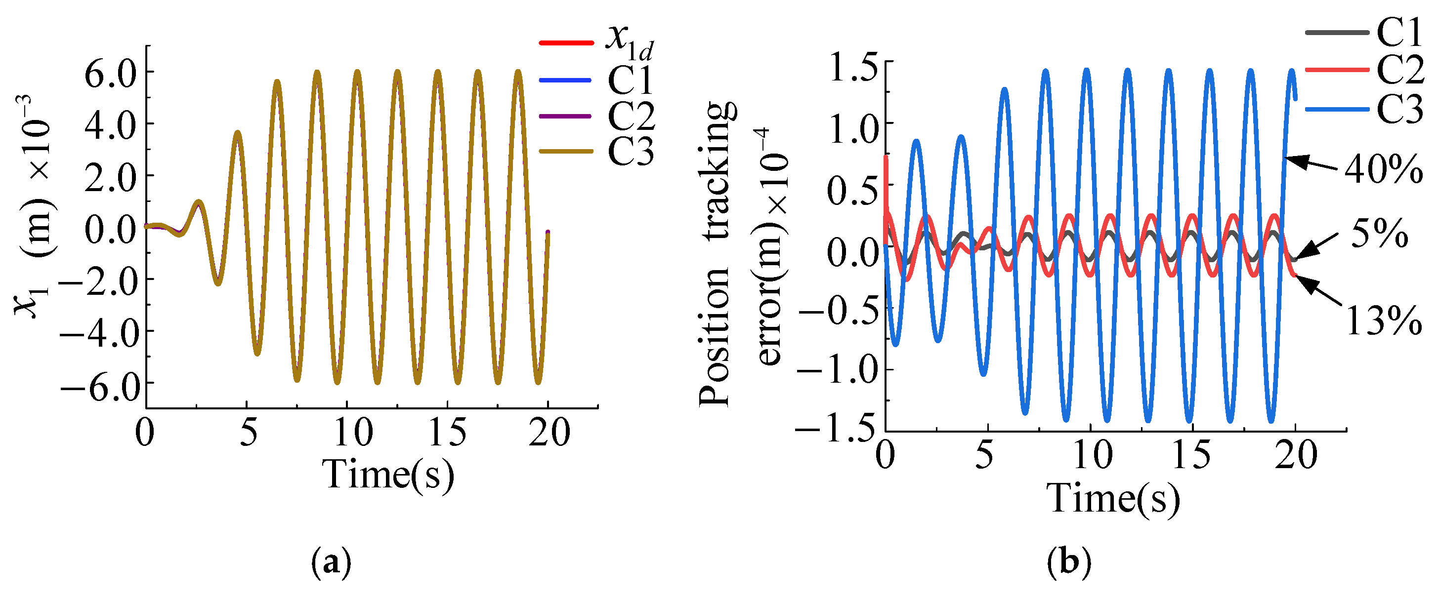
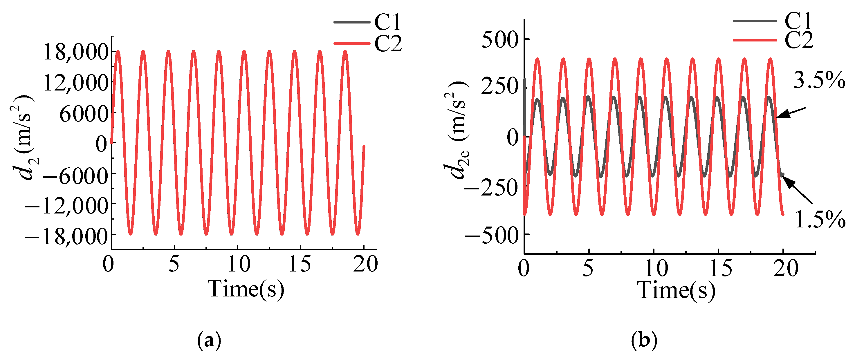
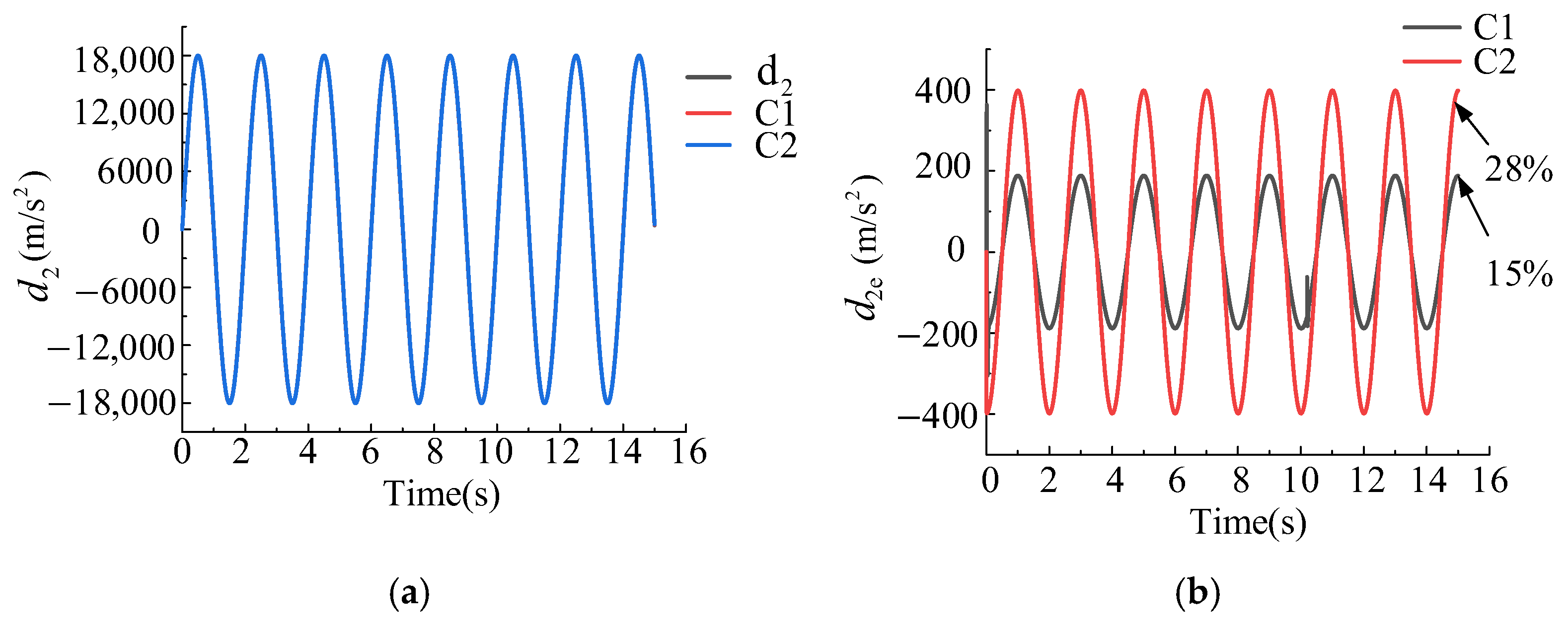
4. Application Verification

To verify the advantages of the output feedback controller mentioned above, a simulation model of a dual-spool electro-hydraulic valve is established. The physical parameters used in the model are shown in Table 2.
In this article, three control schemes are compared, among which control scheme 1 is an output feedback controller designed based on a cascaded linear extended state observer, control scheme 2 is an output feedback controller designed based on a standard structure linear extended state observer, and control scheme 3 is a high-gain PID controller. The specific parameter settings are shown in Table 3.
  • Case 1: Given the external disturbance signal d 2 = 18,000 sin ( 3 . 14 t ) and given the valve core position command signal is x 1 d = 0.03 ( 1 e 0.01 t 3 ) a t a n ( 0.2 s i n ( 3.14 t ) ) .
The tracking performance comparison of three controllers applied to the valve core position is shown in Figure 3. The simulation results depict that the tracking error of the backstepping control based on the system model is significantly smaller than that of the high-gain PID control and for the C3 controller the tracking error is within approximately 40%, for the C2 controller the control error is within about 13%, and for the C1 controller the control error is within roughly 5%. Compared with controller C2 designed based on the standard LESO, controller C1 designed in this paper based on the cascaded structure observer has a better tracking effect on the position of the valve core.
The comparison of the estimation effects of the two observers for the given external disturbance d 2 is collected in Figure 4. According to the position tracking effects of the three different controllers shown in Figure 4a, under the condition of approximate parameters, the estimation effects of the two observers for external disturbances are similar and both observers can achieve low-lag tracking for external disturbances. According to the estimation error reflected in Figure 4b, the estimation error of external disturbance for C1 is within approximately 1.5%, and for C2 the estimation error of external disturbance is within about 3.5%. Therefore, it can be found that due to the cascade structure the observer used in C1 has higher estimation accuracy for external disturbances. This also explains that under the same controller parameters the control error of C1 is smaller.
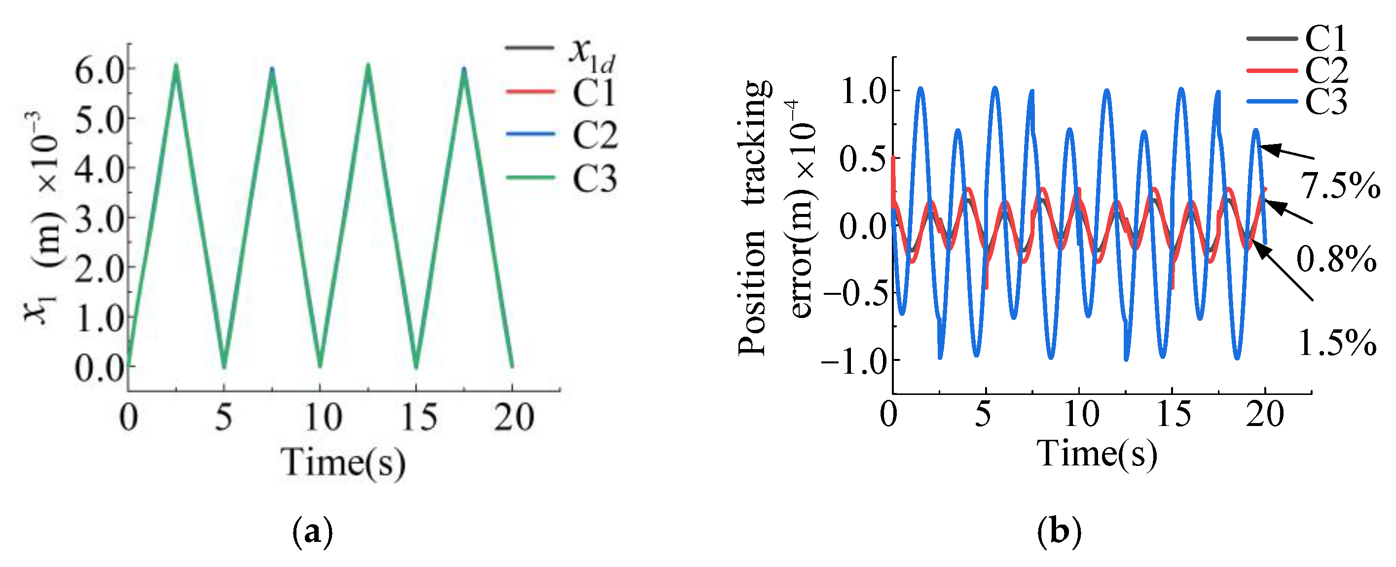
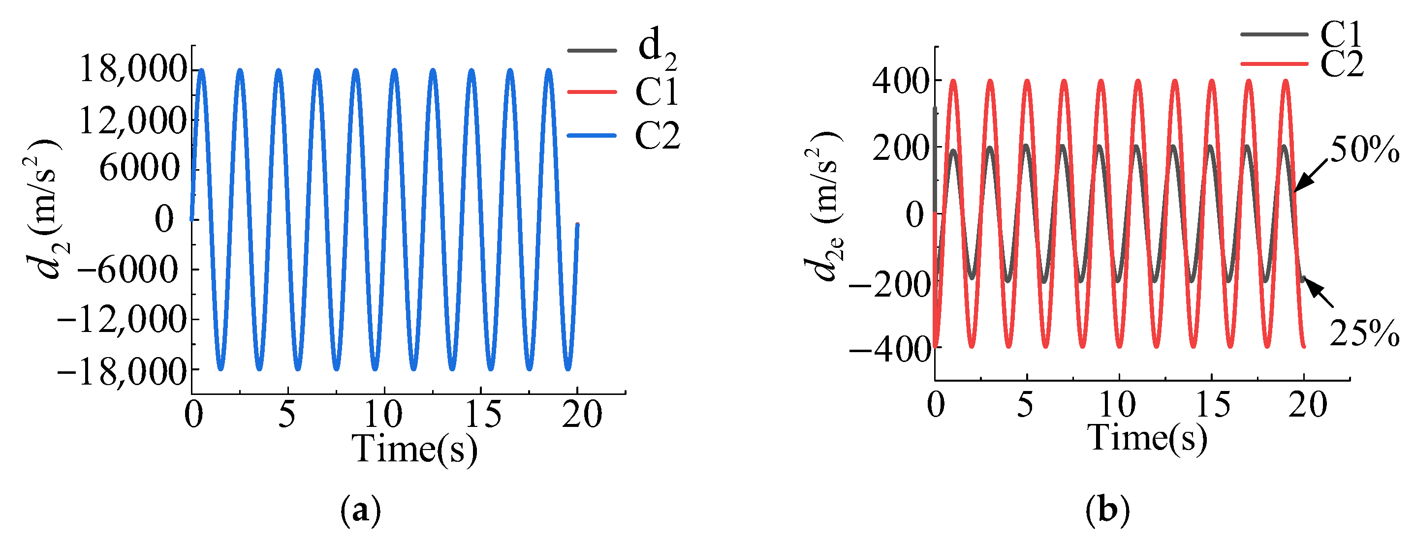
  • Case 2: The given valve core position command signal is a triangular wave with a cycle of 5 s and a stroke of 0–6 mm and the given external disturbance signal is d 2 = 18,000 sin ( 3 . 14 t ) .
Given a triangular wave command for the position x 1 d of the valve core, the comparison of tracking effects using three different controllers is found in Figure 5. The simulation results show that the tracking errors of the two controllers, C1 and C2, based on backstepping control design are significantly smaller than those of the high-gain PID controller C3. For the C3 controller the tracking error is within approximately 7.5%, for the C2 controller the control error is within about 1.5%, and for the C1 controller the control error is within roughly 0.8%. Compared with controller C2 designed based on the standard LESO, controller C1 designed in this paper based on a cascaded structure observer has better tracking performance when faced with speed changes in triangular wave instructions.
The comparison of the estimation performance of the two observers for a given external disturbance is collected in Figure 6. The simulation results show that both observers can achieve good tracking performance for external disturbances and approximate parameters, and the tracking lag of the two observers for external disturbances is almost invisible. According to the estimation error reflected in Figure 6b, the estimation error of external disturbance for C1 is within approximately 25% and for C2 the estimation error of external disturbance is within about 50%. Therefore, it can be observed that due to the cascade structure the observer used in C1 has a smaller estimation accuracy error for external disturbances, which also explains that under the same controller parameters and position instructions the control error of C1 is smaller.
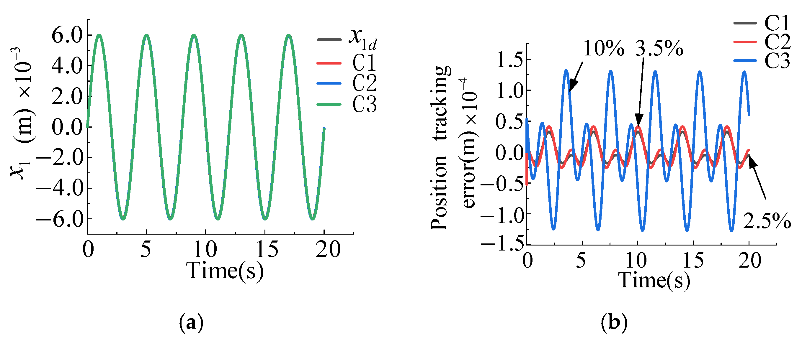
  • Case 3: The given valve core position command signal is x 1 d = 0.006 sin ( 1.57 t ) and the given external disturbance signal is d 2 = 18,000 sin ( 3 . 14 t ) .
The position of the valve core is given a sine signal with a cycle of 4 s and a stroke of 6 mm. The comparison of tracking effects using three different controllers is found in Figure 7. The simulation results depict that the tracking errors of the two controllers, C1 and C2, based on backstepping control design are significantly smaller than those of the high-gain PID controller C3. For the C3 controller the tracking error is within approximately 10%, for the C2 controller the control error is within about 3.5%, and for the C1 controller the control error is within roughly 2.5%. Compared with controller C2, designed based on standard LESO, controller C1 designed in this paper based on cascaded structure observer has better tracking performance when faced with sudden speed changes in triangular wave instructions.
The comparison of the estimation performance of the two observers for a given external disturbance is collected in Figure 8. The simulation results show that both observers can achieve a good tracking performance for external disturbances and approximate parameters, and the tracking lag of the two observers for external disturbances is almost invisible. According to the estimation error reflected in Figure 8b, the estimation error of external disturbance for C1 is within approximately 14.5% and for C2 the estimation error of external disturbance is within about 27%. Therefore, it can be observed that due to the cascade structure the observer used in C1 has a smaller estimation accuracy error for external disturbances, which also explains that under the same controller parameters and position instructions the control error of C1 is smaller.
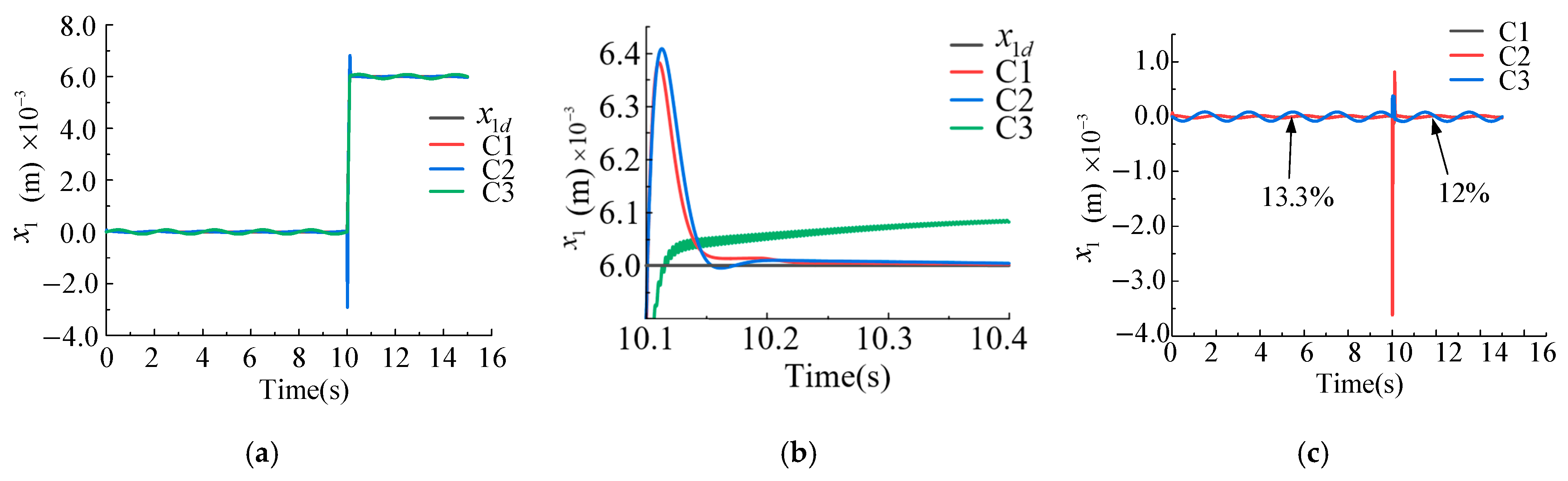
  • Case 4: The given external disturbance signal is d 2 = 18,000 sin ( 3 . 14 t ) , and the given valve core position command signal is x 1 d = 0 0.06 t 0.006 3.24 × 10 8 t t < 10 10 t < 10.1 10.1 t < 50 .
When the input signal is a step signal, Figure 9a shows the tracking effects of three different controllers, while the magnified view of the tracking effects of the three different controllers is presented in Figure 9b, and the tracking error comparison is shown in Figure 9c. The simulation results show that the two controllers, C1 and C2, based on backstepping control design will have significant tracking errors when facing severe mismatches in position states. As can be seen, for the C1 controller the control error is within about 12% and for the C2 controller the control error is within roughly 13.3%. Compared to the controller C2 based on standard LESO design, the controller C1 designed in this article, based on a cascaded structure observer, has a smaller tracking error, while the high-gain PID controller C3 does not show any position mutation through the high-gain coefficient. However, through Figure 9b, it can be observed that the entire system is in an unstable working state.
The comparison of the estimation performance of the two observers for a given external disturbance is depicted in Figure 10. The simulation results indicate that under the condition of approximate parameters both observers can achieve good tracking performance for external disturbances. According to the estimation error reflected in Figure 10b, the estimation error of external disturbance for C1 is within approximately 15% and for C2 the estimation error of external disturbance is within about 38%. Furthermore, it can be observed that due to the cascade structure the observer used in C1 has a smaller estimation accuracy error for external disturbances, which also explains that under the same controller parameters and position instructions the control error of C1 is smaller.

5. Conclusions

In this paper, based on the structure and working principle of a dual-spool electro-hydraulic valve, a linear extended state observer based on a cascade structure is designed. The expected load pressure is synthesized through the expected trajectory, achieving the decoupling of nonlinear coupling phenomena in the state-space equation. On this basis, an output feedback controller is designed based on the backstepping idea. From the stability criterion of uniform exponential stability (USE) it can be seen that the estimation error of the system state for this cascaded observer is convergent. Through the Hurwitz polynomial stability criterion it is proven that the tracking error of the controller designed with this observer for the instruction signal is bounded and convergent. Finally, through extensive simulation case comparisons, in all four working condition tests for spool position tracking performance C1 achieved tracking errors of 5%, 0.8%, 2.5%, and 12%, C2 recorded errors of 13%, 1.5%, 3.5%, and 13.3%, and C3 demonstrated tracking errors of 40%, 7.5%, and 10% with unstable operation. Controllers C1 and C2 designed with backstepping control exhibited significantly smaller tracking errors than controller C3 based on high-gain PID control. In external disturbance estimation tests, C1 achieved estimation errors of 1.5%, 25%, 14.5%, and 15%, while C2 recorded errors of 3.5%, 50%, 27%, and 38%. To sum up, the average tracking error of C1 is about 5.1%, the average tracking error of C2 is about 7.8%, and the average tracking error of C3 is about 19.2%. The average control accuracy of the designed C1 controller is improved by 2.7% and 14.1% compared with C2 and C3, respectively. In terms of the estimation of external disturbances, the average error of C1 is 14% and the average error of C2 is 29.6%. The estimation accuracy of the former is improved by 15.6% compared with the latter. Due to its cascaded structure, C1 achieved over twice the estimation accuracy of C2 for external disturbances, validating the performance of the designed observer and controllers in this paper. Our future research direction is to combine this new structural observer with methods such as state constraints and adaptive control.

Author Contributions

Methodology, C.J., C.A., Z.Y. and Y.J.; software, H.M.; investigation, S.L. and H.M.; writing—original draft, S.L. writing—review and editing, C.J., C.A., X.K. and Z.Y. All authors have read and agreed to the published version of the manuscript.

Funding

This work was supported by the National Natural Science Foundation of China (grant no. 52175065) and the National Natural Science Foundation of China—Regional Innovation and Development Joint Fund (grant no. U22A20178).

Data Availability Statement

The data are contained within the article.

Conflicts of Interest

Authors Cunde Jia and Zhuowei Yu are employed by Beijing Sany Intelligent Manufacturing Technology Co., Ltd. The remaining authors declare that the research was conducted in the absence of any commercial or financial relationships that could be construed as a potential conflict of interest.

Abbreviations

LESOLinear extended state observer
USEUniform exponential stability
IARCIndirect adaptive robust control
DT-SMCDiscrete-time sliding mode controller
ADRCActive disturbance rejection control
GESOGeneralized extended state observer
DCMSSDisturbance compensation motion control system for servo motors
LVDTLinear variable differential transformer
ESOExtended state observer
PIDProportional-integral-derivative
Parameter Explanations
P s Supply pressure
P 1 Left chamber pressure of the main valve
A 1 Pressure bearing area of the left chamber of the main valve
m Main valve core quality
V 1 Volume of the left chamber of the main valve
V 01 Initial volume of the left chamber of the main valve
β e Elastic bulk modulus
u Control input voltage
C d Pilot valve flow coefficient
Q L Load flow rate input to the main valve
P r Return pressure
P 2 Main valve right chamber pressure
A 2 Pressure bearing area of the right chamber of the main valve
B Viscous friction coefficient
V 2 Volume of the right chamber of the main valve
V 02 Initial volume of the right chamber of the main valve
P L = P 1 P 2 Main valve core driving force
k Main valve spring stiffness
ρ Hydraulic oil density
k v Pilot valve electrical gain coefficient
d 1 ( t ) Represents the modeling error including nonlinear friction and the concentrated disturbance caused by external disturbances
d 2 ( t ) System load force modeling error
x State variable
k q Flow gain corresponding to the displacement of the pilot valve core,
P L d Expected load pressure signal
η ˜ n Define error vector
D System modeling error
θ ( t , t 0 ) State-transition matrix of the system
δ ( t ) Disturbance in the system
ϕ 41 Hurwitz matrix
θ Positive-definite matrix

References

  1. Yao, B.; Bu, F.; Reedy, J.; Chiu, G.T.C. Adaptive robust motion control of single-rod hydraulic actuators: Theory and experiments. In Proceedings of the 1999 American Control Conference (Cat. No. 99CH36251), San Diego, CA, USA, 2–4 June 1999; Volume 2, pp. 759–763. [Google Scholar] [CrossRef]
  2. Guan, C.; Pan, S. Nonlinear Adaptive Robust Control of Single-Rod Electro-Hydraulic Actuator with Unknown Nonlinear Parameters. IEEE Trans. Control. Syst. Technol. 2008, 16, 434–445. [Google Scholar] [CrossRef]
  3. Sun, W.; Gao, H.; Yao, B. Adaptive Robust Vibration Control of Full-Car Active Suspensions with Electrohydraulic Actuators. IEEE Trans. Control. Syst. Technol. 2013, 21, 2417–2422. [Google Scholar] [CrossRef]
  4. Mohanty, A.; Yao, B. Indirect Adaptive Robust Control of Hydraulic Manipulators with Accurate Parameter Estimates. IEEE Trans. Control. Syst. Technol. 2011, 19, 567–575. [Google Scholar] [CrossRef]
  5. Wei, Y.; Qian, L.; Nie, S.; Yin, Q. Adaptive Backstepping Sliding Mode Control for Electro-hydraulic Position Servo System of The Artillery Projectile Transfer Arm. In Proceedings of the 2019 IEEE 4th Advanced Information Technology, Electronic and Automation Control Conference (IAEAC), Chengdu, China, 20–22 December 2019; pp. 893–898. [Google Scholar] [CrossRef]
  6. Lin, Y.; Shi, Y.; Burton, R. Modeling and Robust Discrete-Time Sliding-Mode Control Design for a Fluid Power Electrohydraulic Actuator (EHA) System. IEEE/ASME Trans. Mechatron. 2013, 18, 1–10. [Google Scholar] [CrossRef]
  7. Fang, Y.; Jiao, Z.; Wang, W.; Sao, P. Adaptive backstepping sliding mode control for hydraulic servo position systems of rolling mills. J. Electr. Mach. Control. 2011, 15, 95–100. [Google Scholar] [CrossRef]
  8. Guo, Q.; Yin, J.; Yu, T.; Jiang, D. Saturated Adaptive Control of an Electrohydraulic Actuator with Parametric Uncertainty and Load Disturbance. IEEE Trans. Ind. Electron. 2017, 64, 7930–7941. [Google Scholar] [CrossRef]
  9. Yang, G.; Yao, J. Output feedback control of electro-hydraulic servo actuators with matched and mismatched disturbances rejection. J. Frankl. Institute. 2019, 356, 9152–9179. [Google Scholar] [CrossRef]
  10. Han, J. From PID to Active Disturbance Rejection Control. IEEE Trans. Ind. Electron. 2009, 56, 900–906. [Google Scholar] [CrossRef]
  11. Yao, J.; Jiao, Z.; Ma, D. Extended-state-observer-based output feedback nonlinear robust control of hydraulic systems with backstepping. IEEE Trans. Ind. Electron. 2014, 61, 6285–6293. [Google Scholar] [CrossRef]
  12. Zhou, L.; Cheng, L.; Pan, C.; Jiang, Z. Generalized Extended State Observer Based Speed Control for DC Motor Servo System. In Proceedings of the 2018 37th Chinese Control Conference (CCC), Wuhan, China, 25–27 July 2018; pp. 221–226. [Google Scholar] [CrossRef]
  13. Kim, W.; Won, D.; Shin, D.; Chung, C.C. Output feedback nonlinear control for electro-hydraulic systems. Mechatronics 2012, 22, 766–777. [Google Scholar] [CrossRef]
  14. El Yaagoubi, E.H.; El Assoudi, A.; Hammouri, H. High gain observer: Attenuation of the peak phenomena. In Proceedings of the 2004 American Control Conference, Boston, MA, USA, 30 June–2 July 2004; Volume 5, pp. 4393–4397. [Google Scholar] [CrossRef]
  15. Khalil, H.K. High-Gain Observers in Feedback Control: Application to Permanent Magnet Synchronous Motors. IEEE Control. Syst. Mag. 2017, 37, 25–41. [Google Scholar] [CrossRef]
  16. Huang, Y.; Wang, J.; Shi, D.; Wu, J.; Shi, L. Event-Triggered Sampled-Data Control: An Active Disturbance Rejection Approach. IEEE/ASME Trans. Mechatron. 2019, 24, 2052–2063. [Google Scholar] [CrossRef]
  17. Chong, M.S.; Nešić, D.; Postoyan, R.; Kuhlmann, L. Parameter and State Estimation of Nonlinear Systems Using a Multi-Observer Under the Supervisory Framework. IEEE Trans. Autom. Control. 2015, 60, 2336–2349. [Google Scholar] [CrossRef]
  18. Sanfelice, R.G.; Praly, L. On the performance of high-gain observers with gain adaptation under measurement noise. Automatica 2011, 47, 2165–2176. [Google Scholar] [CrossRef]
  19. Astolfi, D.; Marconi, L. A High-Gain Nonlinear Observer with Limited Gain Power. IEEE Trans. Autom. Control 2015, 60, 3059–3064. [Google Scholar] [CrossRef]
  20. Ran, M.; Li, J.; Xie, L. A new extended state observer for uncertain nonlinear systems. Automatica 2021, 131, 109772. [Google Scholar] [CrossRef]
  21. Lin, Z.; Yao, J.; Deng, W. Input constraint control for hydraulic systems with asymptotic tracking. ISA Trans. 2022, 129, 616–627. [Google Scholar] [CrossRef] [PubMed]
  22. Rugh, W.J. Linear System Theory, 2nd ed.; Prentice Hall: Upper Saddle River, NJ, USA, 1996. [Google Scholar]
Figure 1. Structure/hydraulic principle of double-valve core electrohydraulic valve. (a) Structural diagram of the dual-spool electro-hydraulic valve. (b) Hydraulic schematic diagram of the dual-spool electro-hydraulic structure.
Machines 13 00392 g001
Figure 2. Schematic diagram of controller structure.
Machines 13 00392 g002
Figure 3. Comparative analysis of position tracking performance of three controllers. (a) Position tracking effects of three different controllers. (b) Position tracking error of three different controllers.
Machines 13 00392 g003
Figure 4. Estimation of external disturbances and error comparative analysis by two observers. (a) Estimation of external disturbance for two types of observers. (b) Estimation errors of two types of observers for external disturbances.
Machines 13 00392 g004
Figure 5. Comparison of position tracking performance of three controllers: error characteristics analysis. (a) Position tracking effects of three different controllers. (b) Position tracking error of three different controllers.
Machines 13 00392 g005
Figure 6. Comparison of external disturbance estimation and error analysis for two observers. (a) Estimation of external disturbance for two types of observers. (b) Estimation errors of two types of observers for external disturbances.
Machines 13 00392 g006
Figure 7. Comparison of position tracking performance and error characteristics analysis for three controllers. (a) Position tracking effects of three different controllers. (b) Position tracking errors of three different controllers.
Machines 13 00392 g007
Figure 8. Comparison of external disturbance estimation and error analysis for two observers. (a) Estimation of external disturbance by two types of observers. (b) Estimation errors of two types of observers for external disturbances.
Machines 13 00392 g008
Figure 9. Comparison of position tracking performance and error characteristics analysis for three controllers. (a) Position tracking effects of three different controllers. (b) Partial enlarged view of tracking effect. (c) Position tracking error of three different controllers.
Machines 13 00392 g009
Figure 10. Comparison of external disturbance estimation and error analysis for two observers. (a) Estimation of external disturbances using two types of observers. (b) Estimation errors of two types of observers for external disturbances.
Machines 13 00392 g010
Table 1. The parameters used in this paper.
CharacterMeaningCharacterMeaning
P s Supply pressure P r Return pressure
P 1 Left chamber pressure of the main valve P 2 Main valve right chamber pressure
A 1 Pressure bearing area of the left chamber of the main valve A 2 Pressure bearing area of the right chamber of the main valve
m Main valve core quality B Viscous friction coefficient
V 1 Volume of the left chamber of the main valve V 2 Volume of the right chamber of the main valve
V 01 Initial volume of the left chamber of the main valve V 02 Initial volume of the right chamber of the main valve
β e Elastic bulk modulus P L = P 1 P 2 Main valve core driving force
u Control input voltage k Main valve spring stiffness
C d Pilot valve flow coefficient ρ Hydraulic oil density
Q L Load flow rate input to the main valve k v Pilot valve electrical gain coefficient
d 1 Represents the modeling error including nonlinear friction and the concentrated disturbance caused by external disturbances η ˜ n Define error vector
d 2 System load force modeling error D System modeling error
x State variable θ ( t , t 0 ) State-transition matrix of the system
k q Flow gain corresponding to the displacement of the pilot valve core, δ ( t ) Disturbance in the system
P L d Expected load pressure signal ϕ 41 Hurwitz matrix
θ Positive-definite matrix
Table 2. Parameters used in simulation models.
Parameter NameValueParameter NameValue
m (kg)1.05 β e (Pa) 7 × 10 8
A (m2) 4 × 10 4 k (N/m)15,580
V t (m3) 8 × 10 6 B (N/(m/s))350
P s (Pa) 5 × 10 6 P r (Pa)0
k t 4 × 10 8
Table 3. Controller parameters in simulation.
ControllerModel Parameters
C1 ε = 3.3 × 10 4 ,   k 1 = 125 ,   k 2 = 270 ,   k 3 = 500
C2 ω = 3000 ,   k 1 = 125 ,   k 2 = 270 ,   k 3 = 500
C3 k p = 300 ,   k i = 50 ,   k d = 0
Disclaimer/Publisher’s Note: The statements, opinions and data contained in all publications are solely those of the individual author(s) and contributor(s) and not of MDPI and/or the editor(s). MDPI and/or the editor(s) disclaim responsibility for any injury to people or property resulting from any ideas, methods, instructions or products referred to in the content.

