Article

Trajectory Tracking and Driving Torque Distribution Strategy for Four-Steering-Wheel Heavy-Duty Automated Guided Vehicles

School of Mechanical and Power Engineering, Zhengzhou University, Zhengzhou 450001, China
*
Author to whom correspondence should be addressed.
Machines 2025, 13(5), 383; https://doi.org/10.3390/machines13050383
Submission received: 25 March 2025 / Revised: 26 April 2025 / Accepted: 30 April 2025 / Published: 1 May 2025
(This article belongs to the Special Issue Advances in Vehicle Suspension System Optimization and Control)

Abstract

A four-steering-wheel heavy-duty Automated Guided Vehicle (AGV) is prone to lateral instability and wheel slippage during acceleration, climbing, and small-radius turns. To address this issue, a trajectory tracking strategy considering lateral stability and an optimal driving torque distribution strategy considering load transfer and tire adhesion coefficient are proposed. Firstly, a three-degree-of-freedom AGV trajectory tracking model is established, tracking error and sideslip angle are incorporated into the cost function, and an improved model predictive trajectory tracking controller is proposed. Secondly, the longitudinal and yaw dynamic model of AGV is established, and vertical load transfer is analyzed. With the goal of minimizing tire adhesion utilization rate, quadratic programming is used for the optimal distribution of driving torque. Finally, through co-simulation using ADAMS and MATLAB on a narrow “climbing straight+ S-curve” road, the maximum tracking error is 0.0443 m. Compared to the unimproved model predictive control and average driving torque distribution strategy, the sideslip angle is reduced by 58.18%, the maximum tire adhesion utilization rate is reduced by 6.62%, and climbing gradeability on wet roads is enhanced.

1. Introduction

In the era of rapid technological advancement, the wave of intelligent manufacturing is reshaping the global industrial landscape, making efficient material transportation a core aspect of production and manufacturing [1]. Four-steering-wheel Automated Guided Vehicles (AGVs), known for their high load-bearing capacity and ability to perform six types of movements (forward, diagonal, lateral, single Ackermann steering, double Ackermann steering, and pivot steering), have become a research hotspot in the field of logistics AGVs [2,3]. However, due to external disturbances, AGVs may experience lateral instability and partial wheel slippage during climbing, acceleration, deceleration, and turning, causing the vehicle to deviate from the reference path and resulting in failures in efficient, accurate, and reliable handling tasks.
To reduce trajectory tracking errors and avoid lateral instability, scholars have proposed various control schemes, including pure pursuit, fuzzy control, static output feedback (SOF), and model predictive control (MPC) algorithms [4,5,6,7]. The pure pursuit algorithm selects a target point and calculates the steering angle using geometric methods, but the preview distance needs to be dynamically adjusted to prevent error accumulation [8]. Sun et al. [9] proposed a rule for the adaptive adjustment of the preview distance based on steering angle and deflection, reducing tracking errors and oscillations in pure pursuit. Wang et al. [10] integrated fuzzy feedback with the pure pursuit algorithm to compensate for control variables and enhance tracking accuracy, achieving a reduction in lateral deviation by over 50% in curved paths. In [11], a heuristically selected look-ahead point method for pure pursuit was proposed. The point was firstly selected by taking into account the position and the direction of the vehicle and the path; then, it was moved outside the path to address the cutting-corner problem especially in sharp turns. Fuzzy controllers establish rule libraries based on expert experience, fuzzify control variables, perform fuzzy reasoning, and defuzzify to obtain AGV control parameters [12]. Ryoo et al. [13] proposed a new trajectory-tracking control method with a speed regulator based on an interval Type-2 Fuzzy Logic System, achieving a 4.23% lower root mean square error compared to Type-1 Fuzzy Logic Systems. In [14], a fuzzy control pure pursuit algorithm that outputs the actual preview distance by considering factors influencing lateral deviation was introduced. Wang et al. [15] proposed a fault-tolerant tracking control strategy based on the Takagi–Sugeno fuzzy model for the dynamic position control of unmanned ships, considering common actuator failures and bias faults. SOF requires lower demands on vehicle sensor data acquisition, communication speed, and controller online optimization computation speed. It achieves trajectory tracking at low cost by constructing a state observer to estimate the vehicle’s lateral velocity and sideslip angle [16]. In [17], a polytopic linear parameter-varying (LPV) control approach with an SOF control scheme was proposed for path tracking control while considering roll dynamics, demonstrating advantages in driving safety and comfort, and data communication efficiency. In [18], a static robust H∞ output-feedback controller was proposed, and the uncertainty effects of the cornering stiffness and external disturbances were included to improve the robustness of the control scheme. In [19], a static output controller based on a non-compensation parallel distributed technique and a Takagi–Sugeno (T-S) model of vehicle lateral dynamics was proposed to consider the unavailability of some vehicle states. MPC establishes a trajectory tracking error model for AGVs, calculates system outputs and control variables within the prediction horizon, and solves for the optimal control variables at the next moment through rolling optimization [20]. Tang et al. [21] incorporated penalty terms into the objective function to handle inequality constraints and enhance MPC computational efficiency, reducing the average solving time by 5.1% compared to traditional algorithms. Xu et al. [22] presented a trajectory tracking scheme utilizing MPC and preview-follower theory, improving lateral stability by controlling reference lateral acceleration. In [23], an adaptive MPC controller with PSO algorithm optimizing weighting gains of steering control parameters was proposed to solve tire force saturation during an emergency obstacle avoidance. In [24], an MPC-based strategy considering slipping and smoothing was proposed, improving the lateral stability of underwater robots. MPC must ensure the accurate measurement of vehicle state information within each control time step. A feasible approach is to employ state-variable observers or sensor fusion techniques. In [25], an event-triggering-based and low-cost device solution was proposed to estimate the vehicle roll, pitch, and yaw angle under high dynamic conditions to avoid in-vehicle network saturation. In [26], a DNN-embedded robust H∞ observer-based tracking control plan was proposed to resist external disturbance and measurement noise. In [27], an IMM filter was designed first to combine estimates from multiple models, and a multimodal learning approach was used to address the shortcomings of the existing track-to-track fusion techniques. However, existing trajectory tracking strategies primarily focus on path tracking accuracy, yaw rate error, and real-time obstacle avoidance, with stability evaluation metrics such as lateral acceleration and lateral velocity being unsuitable for low-speed, heavy-duty four-steering-wheel AGVs in narrow curves, necessitating further research.
To address the issues of uncoordinated driving force distribution and wheel slippage, scholars have proposed various driving torque distribution algorithms, including the average torque distribution strategy, the tire-dynamic-load-based torque distribution strategy, and the minimum-objective-function-based optimal torque distribution strategy [28]. The average distribution strategy does not consider vertical load transfer, leading to slippage in some wheels due to high adhesion coefficients, while others cannot provide sufficient yaw torque due to low adhesion coefficients [29]. Tire-load-based distribution algorithms consider vertical load transfer during acceleration, deceleration, and steering, enhancing vehicle control stability [30]. Zhang et al. [31] proposed a driving cooperative control strategy based on the torque distribution coefficient method and designed a sliding mode coordination controller for driving torque, reducing yaw rate deviation by 25% and sideslip angle deviation by 23% compared to conventional sliding mode controllers. In [32], in order to minimize the friction between each tire and road surface, and the balance friction among different wheels, an iterative bisection torque distribution method was proposed. Optimal distribution strategies set objective functions based on diverse control requirements, such as vehicle lateral stability, tire slip rate, road adhesion coefficient, and driver intent, achieving optimal driving torque distribution under multiple objectives [33]. Cao et al. [34] proposed a multi-objective optimal torque distribution strategy, considering front and rear axle load transfer and variations in adhesion characteristics, significantly reducing vehicle energy consumption and tire slip rates. In [35], a torque vector control strategy was proposed to distribute longitudinal and lateral tire forces considering the tire information, the driver’s commands, and the signal produced by the yaw rate controller. Liu et al. [36] established a whole vehicle model under centroid variation and a torque distribution control strategy based on a PID neural network, reducing drive motor power and vehicle lateral position deviation. Kim et al. [37] presented a torque matching strategy to set the optimal efficiency point by linearizing the drive efficiency combination of the two motors. However, compared to conventional AGVs, four-steering-wheel heavy-duty AGVs exhibit more significant changes in vertical wheel loads during climbing, acceleration, and deceleration, with each wheel being independently controlled. Therefore, it is necessary to further establish a time-varying model that accounts for the load transfer of each wheel and the tire adhesion coefficients with changes in vehicle kinematic parameters, in order to enhance the control margin.
To address the lateral instability of four-steering-wheel heavy-duty AGVs during trajectory tracking and wheel slippage during acceleration, climbing, and turning, this paper proposes an improved model predictive control (IMPC) trajectory tracking strategy considering lateral stability and an optimal driving torque distribution strategy considering load transfer and the tire adhesion coefficient. The main contributions are as follows: (1) Different motion modes are selected based on steering angles, and a linearized, discretized model of tracking error and sideslip angle is established. An IMPC trajectory tracking strategy considering lateral stability is proposed, significantly reducing the AGV’s sideslip angle within acceptable tracking error ranges compared to unimproved MPC. (2) A vertical load transfer model is established for climbing, acceleration, and turning. Quadratic optimization is used to minimize the adhesion utilization rate, solving the driving torque for the four wheels. Compared to the average distribution algorithm, the proposed strategy significantly reduces the maximum tire adhesion utilization rate during heavy-duty AGV climbing, improving the vehicle’s stability margin.

2. Four-Steering-Wheel Heavy-Duty AGV Platform

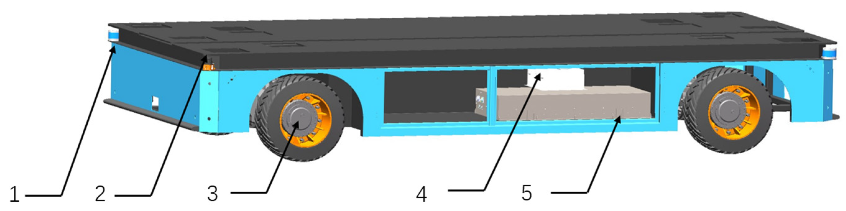
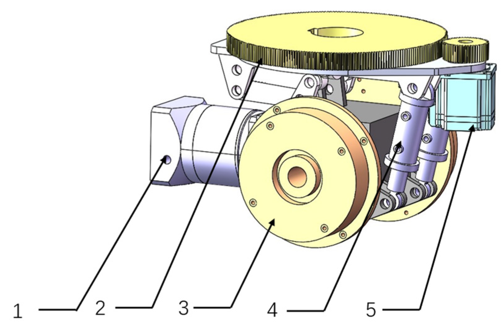
2.1. Overall Mechanical Structure

The structure of the four-steering-wheel heavy-duty AGV is shown in Figure 1. It consists of a load-bearing plate, a welded vehicle body, steering wheel modules, a battery, sensors, and a control system. Considering the factory road conditions and load requirements, the AGV is designed to have a rated load capacity of 5 tons, a certain climbing ability, and omnidirectional movement capabilities. The specific design parameters are listed in Table 1. In Table 1, curb quality is the empty weight of an AGV when fully equipped but without cargo, including the mass of the body, steering wheels, sensors, batteries, and other components; gross quality is the total mass when fully loaded with cargo on the basis of the curb weight, reflecting the vehicle’s load-bearing capacity and design limits.
The steering wheel module adopts a horizontal differential steering wheel assembly, as shown in Figure 2. Each steering wheel shares the vehicle load through two driving wheels, forming a load-bearing structure with eight supporting wheels. The steering wheel is connected to the vehicle body via a steering gear. During operation, the steering motor drives the rotation of the driving wheels to achieve steering. The drive motor is connected to a central gearbox, enabling speed reduction and differential functions to ensure that the driving torque is reasonably distributed between the two driving wheels.
Compared with other conventional drive configurations, e.g., differential-wheel and Mecanum-wheel, the steering-wheel configuration demonstrates distinct advantages. Differential-wheel AGVs feature a simple structural design and convenient steering control [38]. However, they have a large turning radius, making them unsuitable for narrow spaces. Additionally, during steering, the rear wheels passively follow due to elastic deformation, leading to a significant sideslip angle that may cause vehicle fishtailing [39]. Mecanum wheels enable the omnidirectional movement of AGVs [40]. However, the contact area between the rollers and ground is small, and their roller-hub bearings require high precision. Under heavy-load conditions or in environments with dust and debris, Mecanum wheels lack sufficient strength, often resulting in roller and bearing damage [41]. Four-steering-wheel AGVs offer greater load capacity and lower requirements for ground flatness, adjust four-wheel-steering angles and driving forces independently based on turning radius and ground slope, and enable omnidirectional movement, including zero-radius turning. In comparison, four-steering-wheel AGVs exhibit superior adaptability and greater development potential in workshop logistics transportation applications.

2.2. Six Motion Modes of the AGV

By independently controlling the steering angles and driving speeds of different wheels, six motion modes can be achieved:
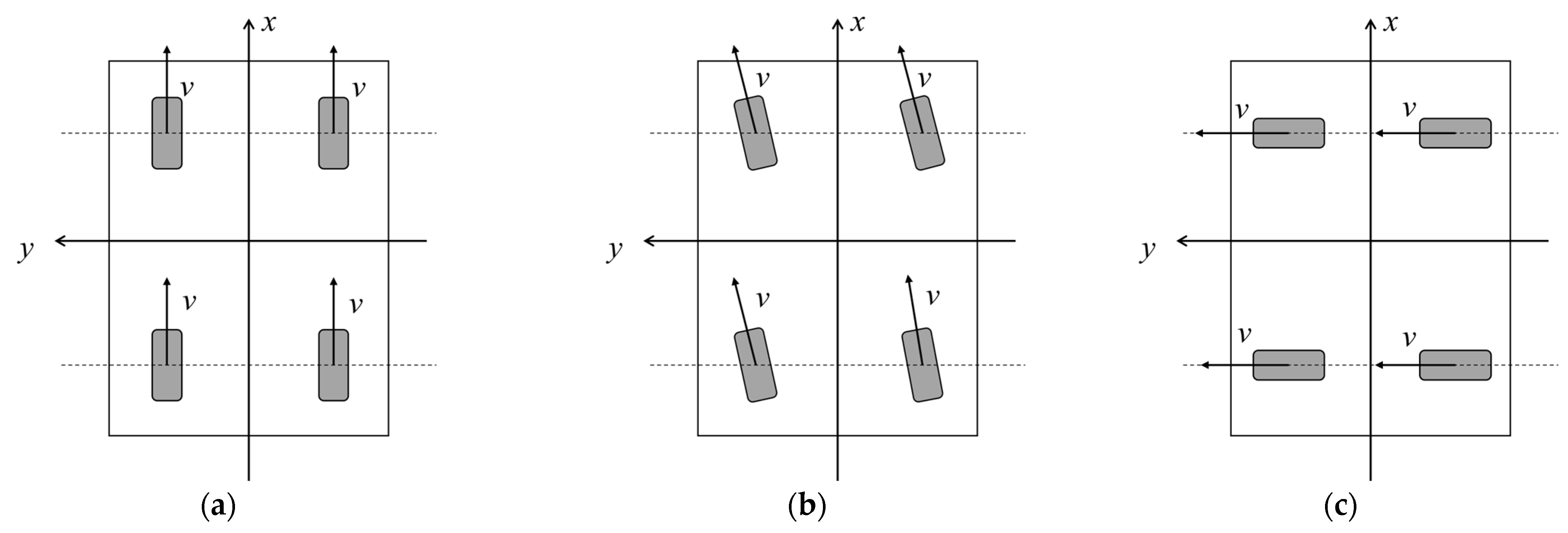
  • Straight-line motion. When all four wheels have the same steering angle and driving speed, the AGV can perform three types of straight-line motions, including forward, diagonal, and lateral movements, as shown in Figure 3.
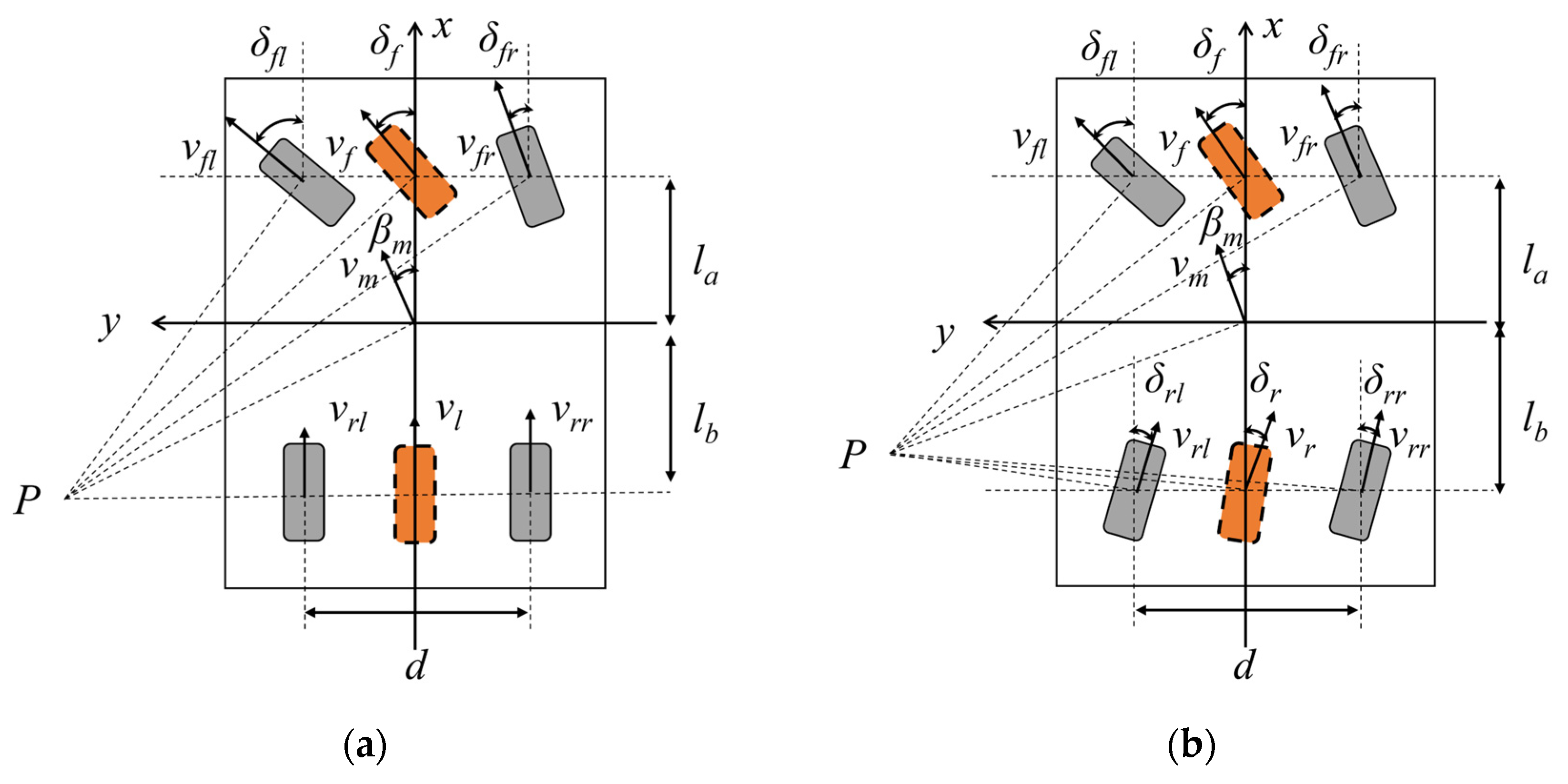
  • Curve motion. By controlling the steering angles and driving speeds of the front and rear steering wheels, two steering modes—single Ackermann steering and double Ackermann steering—can be achieved, as shown in Figure 4. In Figure 4, P is the steering center; l a and l b represent the front and rear wheelbases, respectively; d is the wheel track; δ f l , δ f r , δ r l , and δ r r are the steering angles of the four wheels, respectively; v f l , v f r , v r l , and v r r are the speeds of the four wheels, respectively; ω is the yaw rate; d is the wheel track; v m is the centroid velocity; β m is the sideslip angle of the centroid; the orange wheels represent the equivalent wheels; δ f and δ r are the equivalent front and rare wheel steering angles, respectively; and v f and v r are the equivalent front and rare wheel speeds, respectively.
Under conditions of smooth ground surfaces and low-speed operation, the sideslip angles of the tires can be neglected, and the kinematic model can be constructed with two virtual wheels located on the center line of the main body, namely, front wheel and rear wheel. When the vehicle is in curve motion, from geometric relationships, the correlation between the steering angles of the equivalent wheels and the sideslip angle of the mass center can be derived as:
l a sin ( δ f β m ) = R c cos δ f
l b sin ( β m δ r ) = R c cos δ r
where R c is the turning radius of the center of mass.
The sideslip angle of the centroid can be obtained from Equations (1) and (2):
tan β m = l b tan δ f + l a tan δ r l a + l b
The relationship between the equivalent wheel speeds and the velocity of the center of mass is given by:
v m cos β = v f cos δ f = v r cos δ r
The relationship between the left-front wheel and the equivalent front wheel can be derived from geometric relations as:
R f sin δ f l = d 2 sin ( δ f l δ f )
R f cos β = l a sin ( δ f β )
v f sin δ f = v f l sin δ f l
where R f is the turning radius of the equivalent front wheel.
The steering angle and speed of the left-front wheel can be obtained from Equations (4)–(7):
tan δ f l = tan δ f 1 d 2 l ( tan δ f tan δ r )
v f l = v m tan δ f cos β m sin δ f l
After cargo loading, both the vehicle’s center-of-mass position and wheelbase remain constant. Without requiring precision sensors or state observers, the AGV rapidly estimates its sideslip angle through equivalent steering angles, then distributes corresponding steering angles and speeds to each steering wheel using Equations (10) and (11).
tan δ f l = tan δ f 1 d 2 l ( tan δ f tan δ r ) tan δ f r = tan δ f 1 + d 2 l ( tan δ f tan δ r ) tan δ r l = tan δ r 1 d 2 l ( tan δ f tan δ r ) tan δ r r = tan δ r 1 + d 2 l ( tan δ f tan δ r )
v f l = v m tan δ f cos β m sin δ f l v f r = v m tan δ f cos β m sin δ f r v r l = v m tan δ r cos β m sin δ r l v r r = v m tan δ r cos β m sin δ r r
3
Pivot steering. When the steering angles of the wheels on opposite sides are the same, those on the same side are opposite, and the driving speeds are the same, the AGV pivot-steers around its geometric center, as shown in Figure 5.
The steering angles of the four wheels are determined by the chassis structure:
δ f l = arctan l d δ f r = arctan l d δ r l = arctan l d δ r r = arctan l d

3. IMPC Trajectory Tracking Strategy Considering Lateral Stability

In this section, a three-degree-of-freedom (3DOF) four-steering-wheel AGV trajectory tracking model is established, a cost function that considers tracking error and sideslip angle is proposed, and a trajectory tracking controller based on IMPC is developed.

3.1. Four-Steering-Wheel AGV Trajectory Tracking Model

Based on the following assumptions, a 3DOF four-steering-wheel AGV motion model considering longitudinal, lateral, and yaw motions is established:
  • Roll, pitch, and vertical motions are ignored due to the flat workshop floor.
  • The output steering angle of the steering motor equals the actual wheel steering angle due to the small tire sideslip deformation.
  • The contact between the wheels and the ground is pure rolling without slippage.
  • The front wheel track and rear wheel track of the vehicle are equal.
The 3DOF four-steering-wheel AGV motion model is shown in Figure 6. In Figure 6, xoy represents the global coordinate system, CM is the center of mass, P is the rotation center, (x, y) is the centroid coordinate, and φ is the yaw angle.
In narrow curves, the AGV achieves rapid trajectory tracking through diagonal motion. During diagonal motion, all wheels have the same steering angle, and the driving speed equals the centroid speed:
x ˙ = v m cos ( φ + β m ) y ˙ = v m sin ( φ + β m ) φ = φ 0 β m = δ v w = v m
where φ 0 is the initial yaw angle before diagonal motion, δ is the steering angle, and v w is the wheel driving speed.
On general roads, the steering angles of the front and rear wheels are small and opposite in direction. Double Ackermann steering is used to adjust tracking errors to enhance lateral stability. Assuming δ f + δ r < 30 , the vehicle motion model can be obtained:
x ˙ = v m cos ( φ + β m ) y ˙ = v m sin ( φ + β m ) φ ˙ = v m cos β m ( tan δ f tan δ r ) l β m = l b tan δ f + l a tan δ r l
From Equations (13) and (14), the four-wheel steering AGV can be regarded as a system with input u ( δ f , δ r , v m ) and state X ( x , y , φ ) :
X ˙ = f ( X , u )
The reference trajectory includes the reference pose state X r e f , the reference speed, and the steering angle u r e f required for trajectory tracking:
X ˙ r e f = f ( X r e f , u r e f )
By performing a Taylor expansion, the linearized motion model of the four-steering-wheel AGV relative to the reference trajectory is obtained:
X ˙ = f ( X r e f , u r e f ) + f ( X , u ) X ( X X r e f ) + f ( X , u ) u ( u u r e f )
Subtracting Equation (17) with (16) and discretizing them, the linearized deviation model of the AGV’s current position and heading angle relative to the reference trajectory is obtained:
X ˜ ( k + 1 ) = A k , t X ˜ ( k ) + B k , t u ˜ ( k )
where
A k , t = 1 0 v m r e f T sin ( φ r e f + β m r e f ) 0 1 v m r e f T cos ( φ r e f + β m r e f ) 0 0 1
B k , t = v m r e f t sin ( φ r e f + β m r e f ) 2 v m r e f t sin ( φ r e f + β m r e f ) 2 cos ( φ r e f + β m r e f ) t v m r e f t sin ( φ r e f + β m r e f ) 2 v m r e f t sin ( φ r e f + β m r e f ) 2 sin ( φ r e f + β m r e f ) t k 1 t k 2 t k 3 t
k 1 = v m r e f ( cos β m r e f sec 2 δ f r e f l sin β m r e f ( tan δ f r e f tan δ r r e f ) l b ) l 2
k 2 = v m r e f ( cos β m r e f sec 2 δ r r e f l + sin β m r e f ( tan δ f r e f tan δ r r e f ) l a ) l 2
k 3 = cos β m r e f l ( tan δ f r e f tan δ r r e f )
Here, X ˜ is the discretized state variable, u ˜ is the discretized control variable, t is the sampling interval, x r e f is the reference trajectory’s x-coordinate, y r e f is the reference trajectory’s y-coordinate, φ r e f is the reference trajectory’s heading angle, v m r e f is the reference centroid speed, β m r e f is the reference centroid sideslip angle, δ f r e f is the reference equivalent front steering angle, and δ r r e f is the reference equivalent front steering angle.
The state variables and control variables are combined into a new state variable to simplify the form of the cost function:
ξ ( k | t ) = X ˜ ( k | t ) u ˜ ( k 1 | t )
ξ ( k + 1 | t ) = A ˜ k , t ξ ( k | t ) + B ˜ k , t Δ u ( k | t )
where
ξ ( k + 1 | t ) = A ˜ k , t ξ ( k | t ) + B ˜ k , t Δ u ( k | t )
Within the prediction horizon, the control variables change minimally, and the parameters in the vehicle model remain constant:
A k , t = A t , t ,   k = 1 , 2 , t + N 1 B k , t = B t , t ,   k = 1 , 2 , t + N 1
The system’s output within the prediction horizon is:
Y ( t ) = Φ t ξ ( t | t ) + Θ t Δ u ( t | t )
where
Y ( t ) = ξ ( t + 1 | t ) ξ ( t + 2 | t ) ξ ( t + N c | t ) ξ ( t + N p | t ) Φ t = A ˜ t , t A ˜ t , t 2 A ˜ t , t N c A ˜ t , t N p Δ u ( t | t ) = Δ u ( t + 1 | t ) Δ u ( t + 2 | t ) Δ u ( t + N c | t )
Θ t = B ˜ t , t 0 0 A ˜ t , t B ˜ t , t B ˜ t , t 0 A ˜ t , t N c B ˜ t , t A ˜ t , t N c 1 B ˜ t , t A ˜ t , t N c 2 B ˜ t , t A ˜ t , t N p 1 B ˜ t , t A ˜ t , t N p 2 B ˜ t , t A ˜ t , t N p 3 B ˜ t , t 0 0 A ˜ t , t B ˜ t , t A ˜ t , t N p N c 1 B ˜ t , t

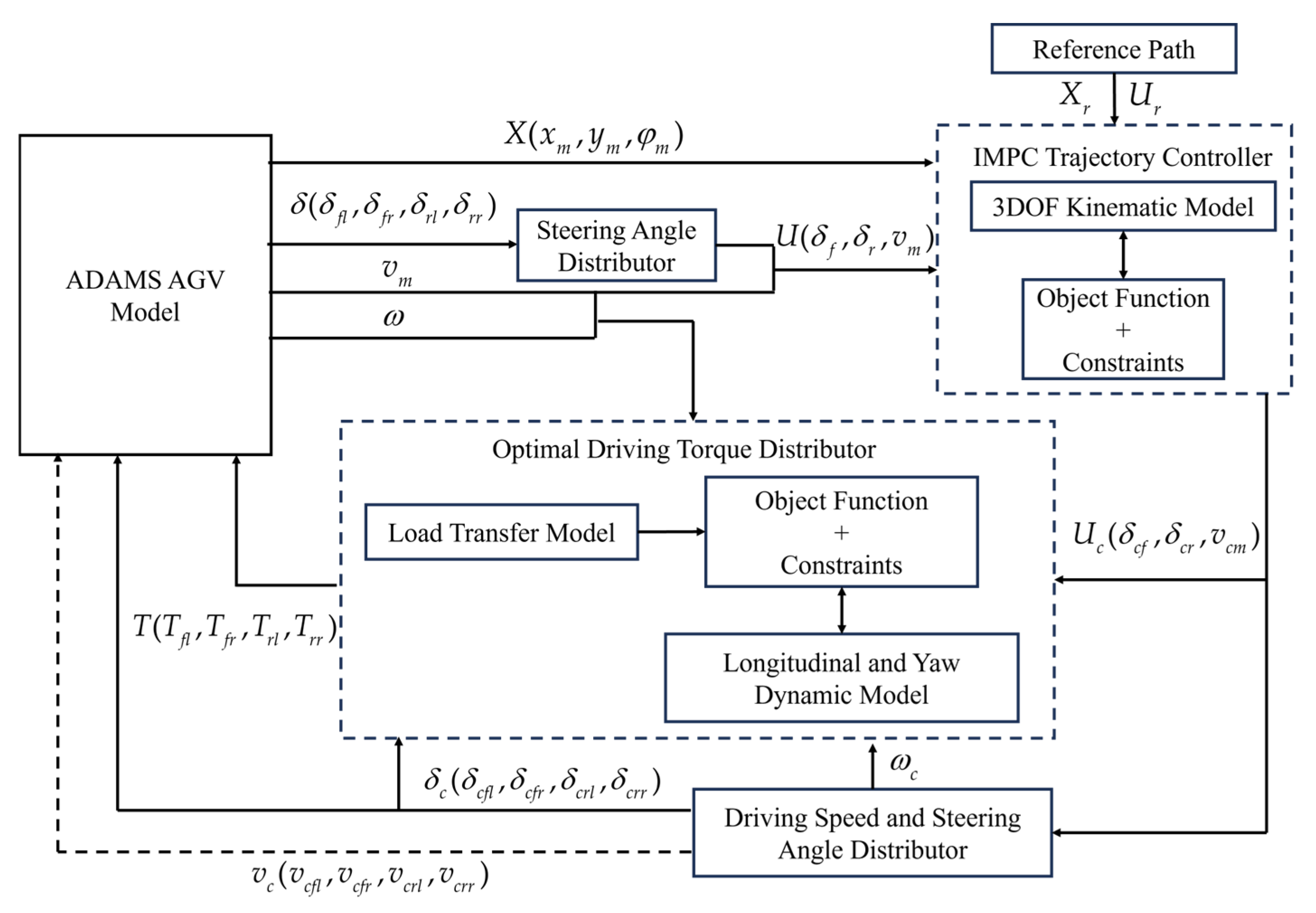
3.2. IMPC Trajectory Tracking Controller

Considering the AGV’s tracking error from the target trajectory, lateral stability, and the continuity of control input, a cost function is established:
J ( k ) = i = 1 N p ξ ( k + i | t ) ξ r e f ( k + i | t ) Q 2 + i = 1 N c ( Δ u ( k + i | t ) R 2 + P u ( k + i | t ) W 2 )
where Q is the tracking error weight matrix, R is the control input continuity weight matrix, W is the centroid sideslip angle weight matrix, and P u is the centroid sideslip angle.
Substituting Equations (19)–(22) into the cost function and ignoring constant terms, Equation (17) is converted to:
J = Δ u T ( Θ t T Q q Θ t + R r + P p W w P p ) Δ u + 2 ( e t T Q q Θ t Y r e f T Q q Θ t ) Δ u
where the symbol represents the Kronecker product,
Q q = 1 N p Q ,   R r = 1 N p R ,   W w = 1 N p W ,   e t = Φ t ξ ( t ) , P p = l b l a 0 0 0 0 0 0 l b l a l b l a 0 0 0 0 l b l a l b l a l b l a l b l a N c × 2 N c
The term ( P p Δ u ) T W w P p Δ u in the cost function restricts the vehicle’s centroid sideslip angle to ensure lateral stability during turning.
To prevent the occurrence of infeasible solutions, soft constraints are added to the cost function:
J = [ Δ u T , ε ] H t [ Δ u T , ε ] T + G t [ Δ u T , ε ] T
where
H t = Θ t T Q q Θ t + R r + P p W w P p 0 0 ρ   G t = [ e t T Q q Θ t Y r e f T Q q Θ t , 0 ]
Due to constraints related to the vehicle and steering wheel motor parameters, the input values and their increments for the front and rear wheel steering angles and centroid speed control have feasible ranges, expressed as:
Δ U min Δ U t Δ U max U min S Δ U t + U t U max
where U t is the sequence of control inputs, Δ U t is the sequence of control input increments, U min is the sequence of minimum control input values, U max is the sequence of maximum control input values, Δ U min is the sequence of minimum control input increments, and Δ U max is the sequence of maximum control input increments.
U t = 1 N c u ( k 1 )   S = 1 0 0 0 1 1 0 0 1 1 1 1 N c × N c
The interior-point method is used to obtain the optimal solution vector u ( δ f , δ r , v m ) of the cost function, which is used as the input for the driving torque distribution algorithm. By controlling the speed and driving torque of the four steering wheel motors, the stable tracking of the reference path is achieved under the condition of minimizing the centroid sideslip angle.

4. Optimal Driving Torque Distribution Strategy Considering Load Transfer and Tire Adhesion Coefficient

The driving torque distribution strategy, based on the vehicle’s load distribution and motion state, adopts an optimal distribution mode that minimizes the objective function. This ensures that the vehicle does not experience slippage while generating sufficient yaw torque, thereby reducing the maximum tire adhesion utilization rate and improving the stability margin of the control system.

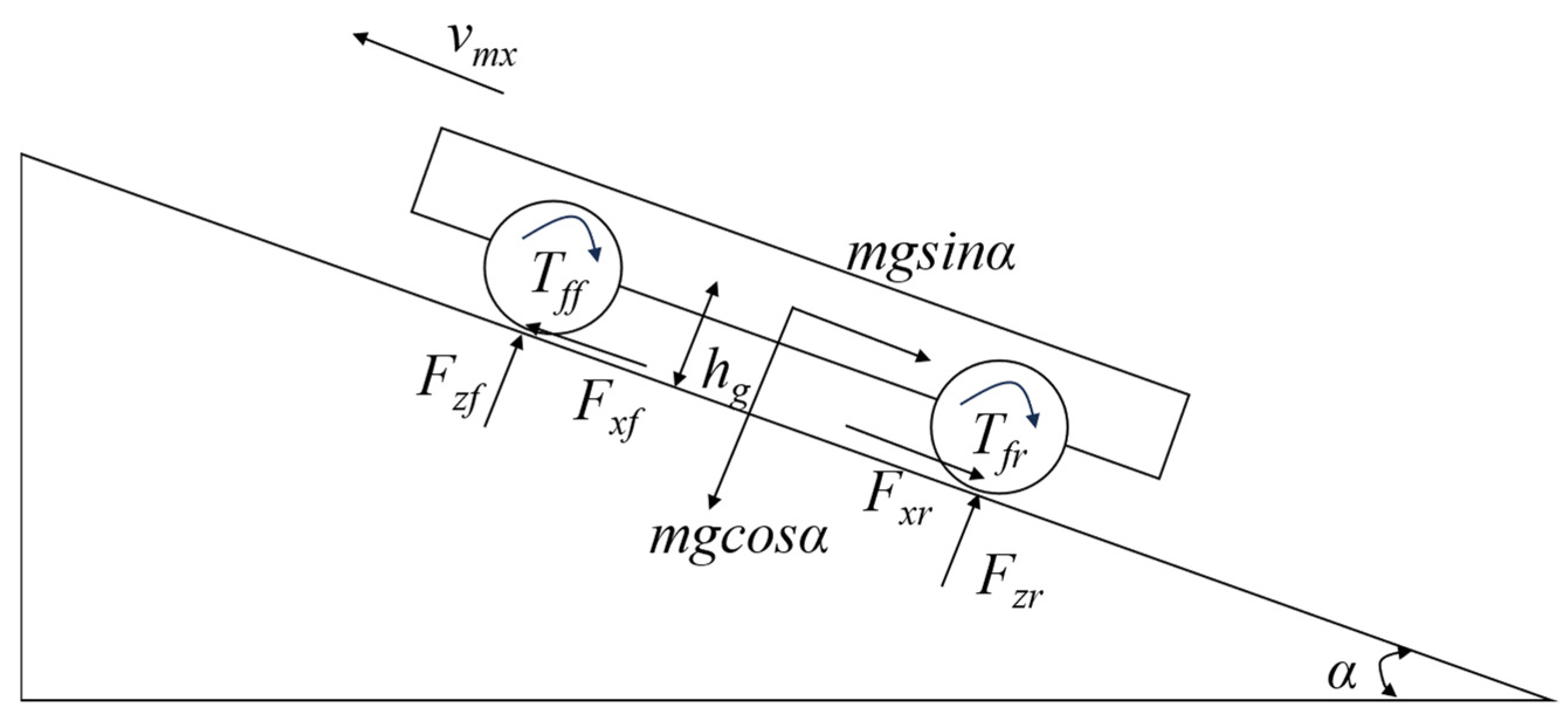
4.1. Four-Steering-Wheel AGV Dynamic Model

During material transportation, the vehicle’s acceleration, deceleration, and turning are performed separately. Therefore, the longitudinal and yaw dynamics should be modeled independently, as shown in Figure 7. In Figure 7, F x f l , F x f r , F x r l and F x r r are the longitudinal forces of the four wheels, respectively; F y f l , F y r l , F y f r and F y r r are the lateral forces of the four wheels, respectively; and I z is the moment of inertia.
  • Longitudinal dynamics:
m v ˙ m x = F x f l cos δ f l F y f l sin δ f l + F x f r cos δ f r F y f r sin δ f r + F x r l cos δ r l F y r l sin δ r l + F x r r cos δ r r F y r r sin δ r r
2.
Yaw dynamics:
I z ω ˙ = l a ( F x f l sin δ f l + F y f l cos δ f l + F x f r sin δ f r + F y f r cos δ f r ) l b ( F x r l sin δ r l + F y r l cos δ r l + F x r r sin δ r r + F y r r cos δ r r ) d 2 ( F x f l cos δ f l F y f l sin δ f l F x f r cos δ f r + F y f r sin δ f r + F x r l cos δ r l F y r l sin δ r l F x r r cos δ r r + F y r r sin δ r r )
From Equations (21) and (22), the total driving torque and yaw moment of the vehicle are influenced by both the longitudinal and lateral forces of the wheels. However, only the longitudinal forces can be controlled through the output torque of the steering wheel drive motors. When the yaw moment increases, the vehicle tends to oversteer. When the yaw moment decreases, the vehicle tends to understeer. By controlling the driving torque of the four steering wheels, the yaw moment of the AGV can be controlled, thereby improving the vehicle’s lateral stability. Let:
F = [ F x , M z ] T T = [ T f l , T f r , T r l , T r r ] T
θ = 1 r cos δ f l 1 r cos δ f r 1 r cos δ r l 1 r cos δ r r k 4 k 5 k 6 k 7
k 4 = 1 r ( l a sin δ f l d 2 cos δ f l )       k 5 = 1 r ( l a sin δ f r + d 2 cos δ f r )
k 6 = 1 r ( l b sin δ r l + d 2 cos δ r l )       k 7 = 1 r ( l b sin δ r r + d 2 cos δ r r )
where r is the wheel radius; F x is the total longitudinal driving force; M z is the total yaw moment; T f l , T f r , T r l , and T r r are the driving torques of the four steering wheels, respectively; and θ is the chassis parameter matrix.
The equality constraints are derived from the vehicle dynamic model:
F = θ T
To improve the stability margin of the vehicle control, the ratio of the driving force provided by each wheel to the maximum adhesion force is selected as the objective function:
J = F x i 2 ( μ F z i ) 2
where F x i is the longitudinal force of each wheel, F z i is the vertical force of each wheel, and μ is the adhesion coefficient.
The objective function represents the ratio of the current longitudinal force on the wheel to the maximum adhesion force. By optimizing the solution to reduce the cost function, the adhesion utilization rate of the wheels can be improved, thereby enhancing the vehicle’s stability.

4.2. Optimal Driving Torque Distributor

The distribution of driving torque is not only related to the driving torque provided by the motors but also to the ground adhesion coefficient and the vertical load on the wheels. During steering, the vertical loads on the inner and outer wheels are not equal. During acceleration and climbing, the vertical loads on the front and rear wheels are also unequal. Considering the changes in vertical load on each wheel during the driving torque distribution process can prevent tire slippage and improve the overall stability of the AGV.
The rolling resistance coefficient of the AGV tires on dry cement pavement is f = 0.018 ~ 0.02 [42]. The rolling resistance torque and its influence on vertical load transfer are negligible compared to the effects of longitudinal/lateral acceleration resistance and climbing resistance. By analyzing the moment balance of the forces acting on the vehicle, a vertical load transfer model is established, as shown in Figure 8. In Figure 8, F z f and F z r are the vertical loads on the front and rear wheels, respectively; F x f and F x r are the longitudinal forces on the front and rear wheels; T f f and T f r are the rolling resistance torques on the front and rear wheels; α is the road slope angle; and h g is the height of the vehicle’s center of mass from the ground when fully loaded.
Set F z f l , F z f r , F z r l and F z r r as the vertical loads on the four wheels, respectively; the relationship between vertical loads and motion parameters can be obtained:
F z f l = m 2 ( g l ( l b cos α h g sin α ) v ˙ m x h g 2 l d v ˙ m y h g )
F z f r = m 2 ( g l ( l b cos α h g sin α ) v ˙ m x h g + 2 l d v ˙ m y h g )
F z r l = m 2 ( g l ( l a cos α + h g sin α ) + v ˙ m x h g 2 l d v ˙ m y h g )
F z r r = m 2 ( g l ( l a cos α + h g sin α ) + v ˙ m x h g + 2 l d v ˙ m y h g )
From the wheel friction circle model, the inequality constraints for the driving torque are obtained:
T i r 2 + F y i 2 ( μ F z i ) 2
where T i is the driving torque of each wheel and F y i is the lateral force of each wheel.
Another inequality constraint for the driving torque is derived from the parameters of the steering wheel drive motors:
T max < T < T max
The cooperative driving torque distribution problem for the four-steering-wheel AGV can be transformed into a quadratic optimization (QP) problem.
Objective function:
J = min T T T K T
Constraints:
F = θ T T i r 2 + F y i 2 ( μ F z i ) 2 T max < T < T max
where
K = 1 ( μ F z f l ) 2 1 ( μ F z f r ) 2 1 ( μ F z r l ) 2 1 ( μ F z r r ) 2
The interior-point method is used to solve the quadratic programming problem, and the optimal distribution scheme for the driving torque is obtained, minimizing the adhesion utilization rate under load transfer conditions.

5. Results and Discussion

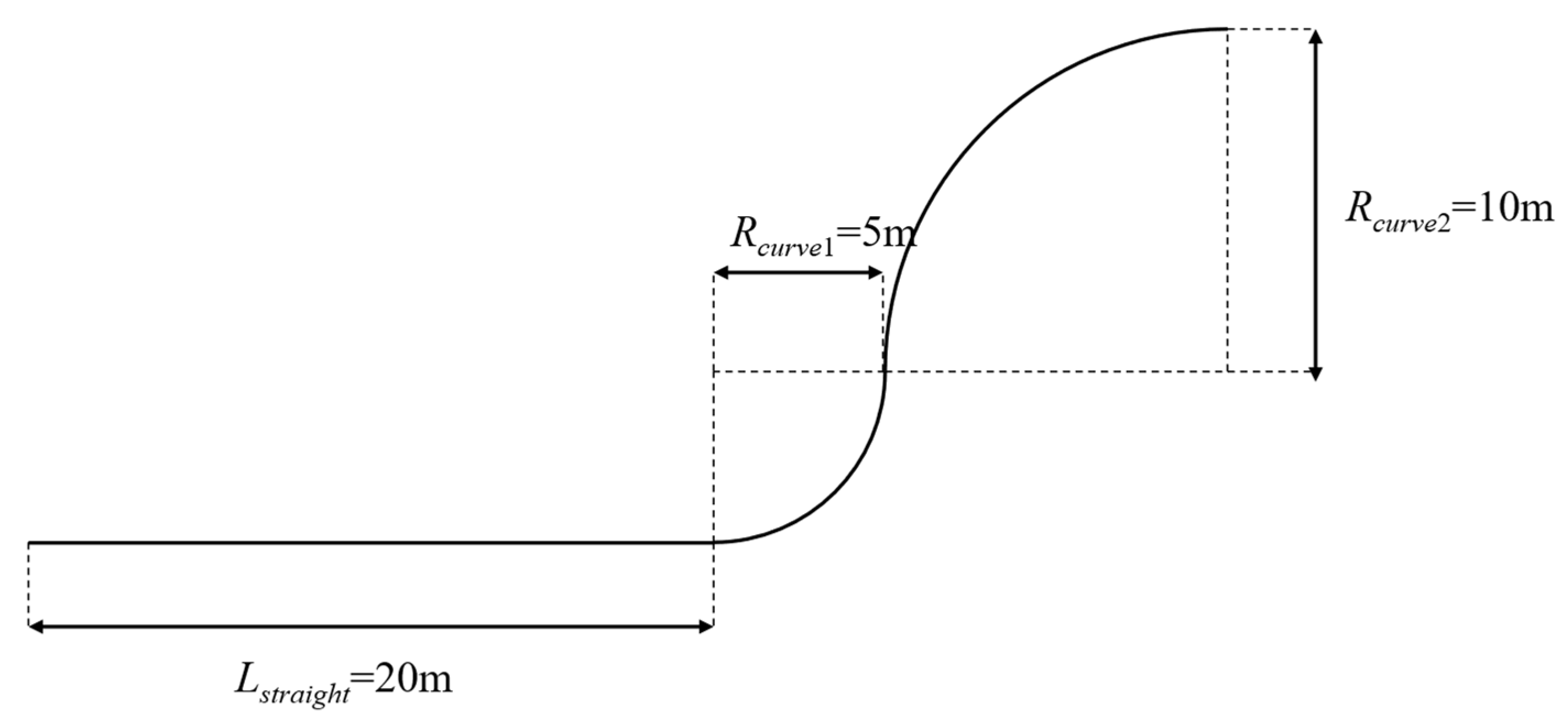
5.1. Introduction to Simulation Scheme

A co-simulation based on ADAMS (version 2020) and MATLAB (version R2022a) is used to validate the proposed trajectory tracking and driving torque distribution algorithms. The simulation model consists of four parts: the ADAMS AGV model, the driving speed and steering angle distributor, the IMPC trajectory tracking controller, and the optimal driving torque distribution controller, as shown in Figure 9.
  • The ADAMS AGV model was configured with parameters in Table 2. The model features eight inputs (set steering angles and driving torques/speeds for all four steering wheels) and nine outputs (center-of-mass longitudinal/lateral positions, yaw angle, velocity, yaw rate, and steering angles of four wheels). Each steering wheel is simplified into two components, a steerable wheel and a driving wheel, and is connected to the vehicle body via another revolute joint. The complete model consists of nine moving parts, three fixed paths, eight revolute joints, eight tire–ground contact pairs, and six DOF in total. Considering the heavy-load condition, low operating speed, only three DOF are practically active during motion: longitudinal, lateral, and yaw. The steerable wheels employ position-driven control while the driving wheels use torque control to simulate the AGV’s dynamic behavior.
  • The driving speed and steering angle distributor performs bidirectional conversion between the complete kinematic vehicle model and the equivalent wheel model.
  • The IMPC trajectory tracking controller was developed to holistically consider both the AGV’s trajectory tracking error and the center-of-mass sideslip angle. Through a receding horizon optimization approach, it generates real-time control commands for the equivalent steering wheels at each time step.
  • The optimal driving torque distribution controller holistically accounts for both load transfer effects and tire adhesion coefficient. Through QP optimization, it distributes torque to four steering-wheel motors.
Dry concrete pavement was selected as the simulation road. The simulation road consists of a climbing straight section, a sharp curve with a small turning radius (Curve 1), and a gentle curve with a large turning radius (Curve 2), forming a “climbing straight + S-curve” road. The road width is comparable to the AGV size, simulating narrow roads in factory areas. The road environment is shown in Figure 10, and the specific parameters are listed in Table 3.
After inputting the reference trajectory, the vehicle invokes the trajectory tracking algorithm to obtain the current required equivalent steering angles for the front and rear wheels and the centroid speed. These data are used as inputs for the wheel driving speed and steering angle distributor to obtain the steering angles and speeds of the four wheels. Finally, the optimal driving torque distribution controller is used to distribute torque among the four wheels.

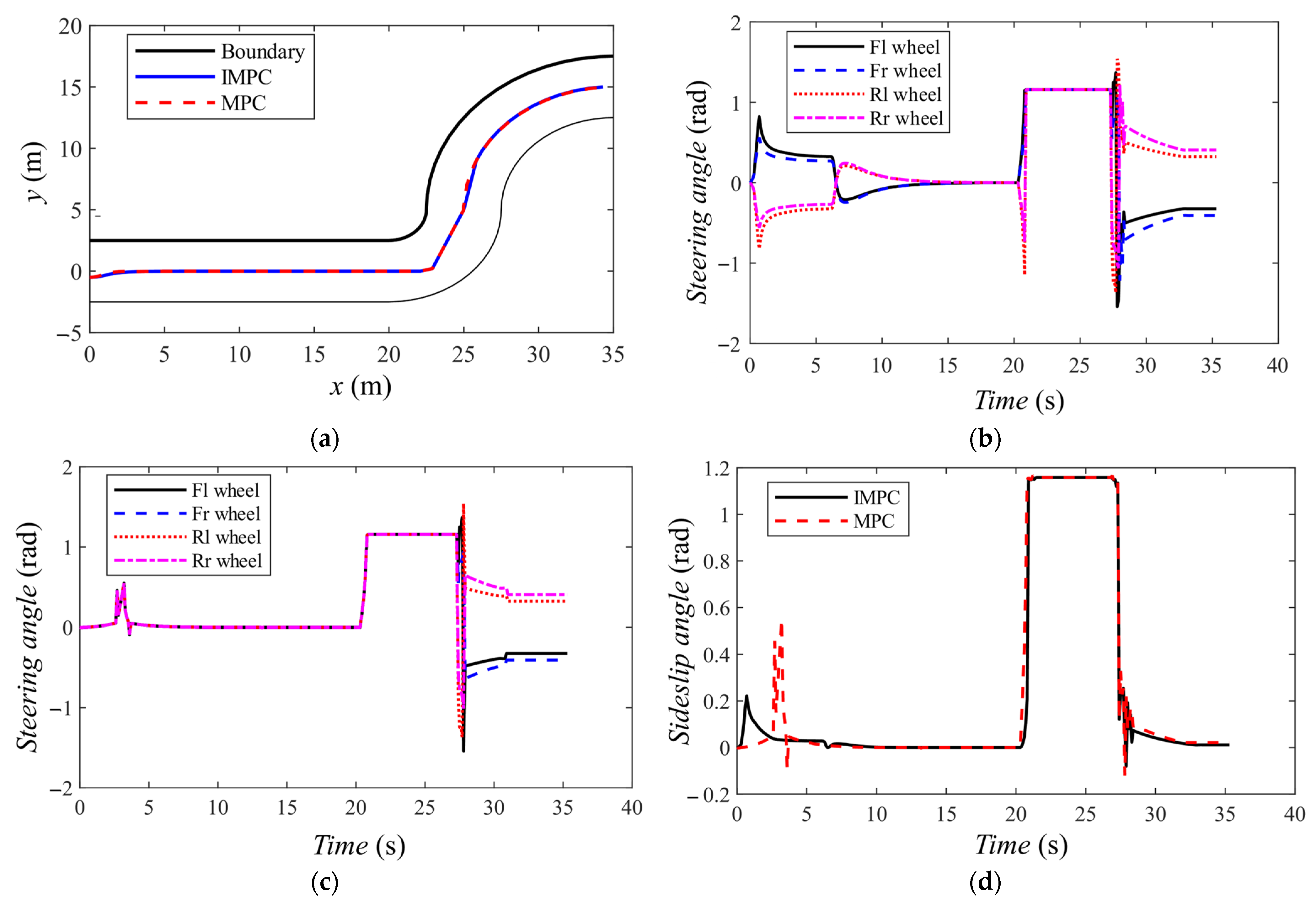
5.2. IMPC Trajectory Tracking Simulation

The trajectory tracking algorithm simulation uses IMPC proposed above and MPC considering lateral acceleration proposed in [22] to track the same trajectory and compares the differences in vehicle tracking error and centroid sideslip angle.
The movement processes of AGV are as followed: The AGV’s initial position is (0, −0.5, 0), with a speed of 0 and front and rear steering angles of 0. During trajectory tracking, the maximum acceleration is 0.2 m/s2. On the climbing straight section, the target speed is 2 m/s, and the AGV accelerates from stationary, maintaining the highest possible speed. On Curve 1, which has a small radius, the AGV passes diagonally, with a target speed of 1 m/s during stable diagonal motion and 0.5 m/s when changing the diagonal direction to reduce the impact of motor control errors on trajectory tracking deviation. On Curve 2, which has a large radius, the target speed is 2 m/s, and the vehicle maintains the highest possible speed. The simulation results for trajectory tracking are shown in Figure 11, and the tracking errors for the reference path are shown in Table 4.
Table 4 shows that during trajectory tracking, the max steady-state tracking error is 0.0443 m in the Curve 2 section. The tracking errors of the IMPC strategy are acceptable.
Figure 11 illustrates the variation in the sideslip angle at the center of mass under two trajectory-tracking control strategies, reflecting the vehicle’s lateral stability. During the straight climbing section, the AGV’s significant initial deviation results in a notable difference in sideslip angles between the two control strategies. In the sharp Curve 1, diagonal motion is used to prevent collisions with road boundaries. However, this steering mode inevitably induces a large sideslip angle, which can only be mitigated by adjusting the reference path—a task involving path planning and thus beyond the scope of this study. When entering the wide Curve 2, the AGV exhibits minimal deviation from the reference trajectory, with yaw angle deviation becoming the dominant factor. Both control strategies successfully track the reference path with a small sideslip angle in this segment.
Excluding the diagonal motion, the results demonstrate that the MPC controller based on lateral acceleration exhibits poor stability, with sudden changes in the centroid sideslip angle, reaching a maximum of 0.55 rad. In contrast, the IMPC controller, which considers the sideslip angle of the centroid, tends to use a fixed-ratio double Ackermann steering method, with a maximum centroid sideslip angle of 0.23 rad. Compared to the MPC controller, a reduction of 58.18% in the maximum centroid sideslip angle significantly improves the vehicle’s lateral stability. The results show that the IMPC controller considering the sideslip angle is more suitable for heavy-duty low-speed AGV trajectory tracking.

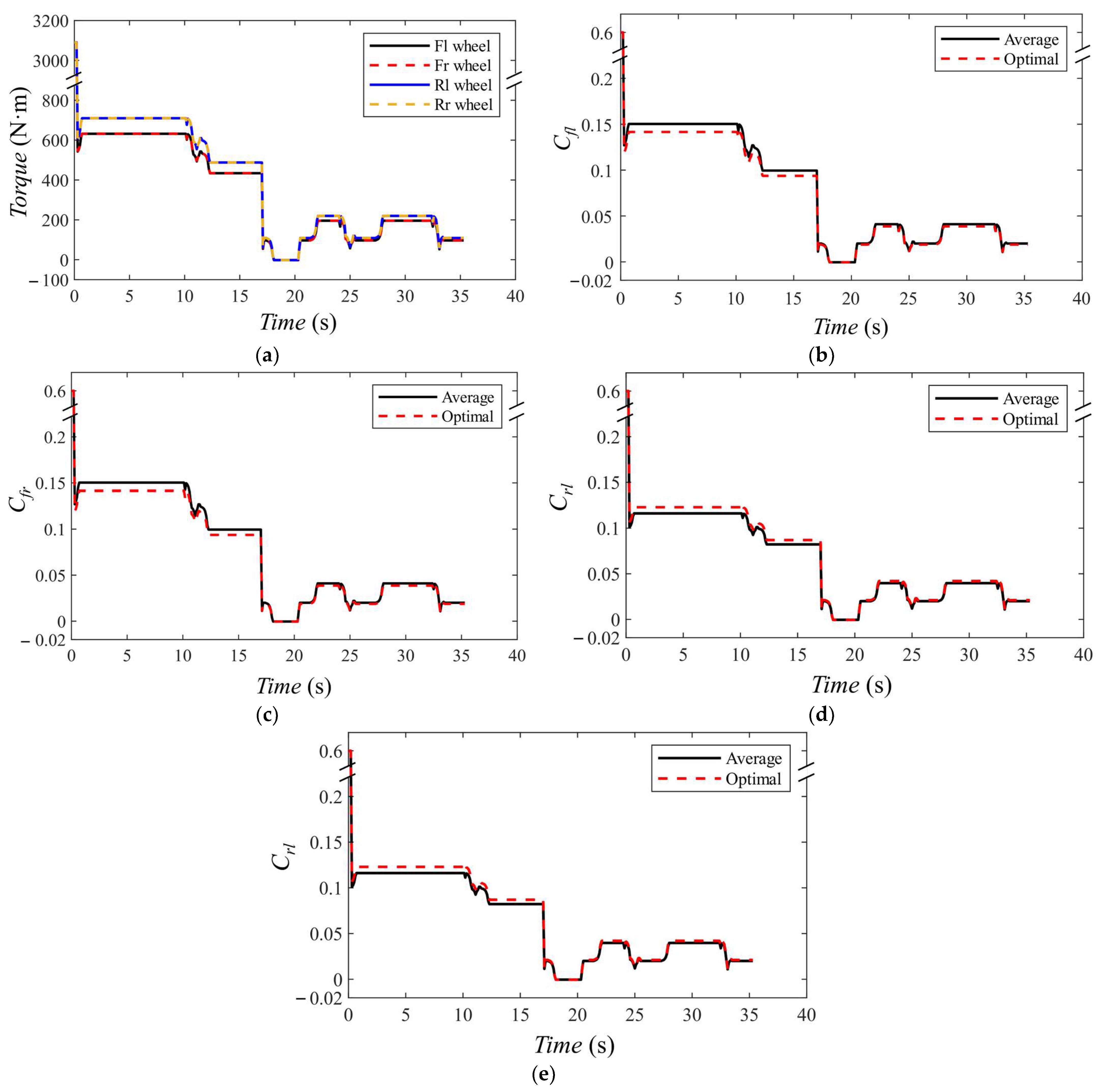
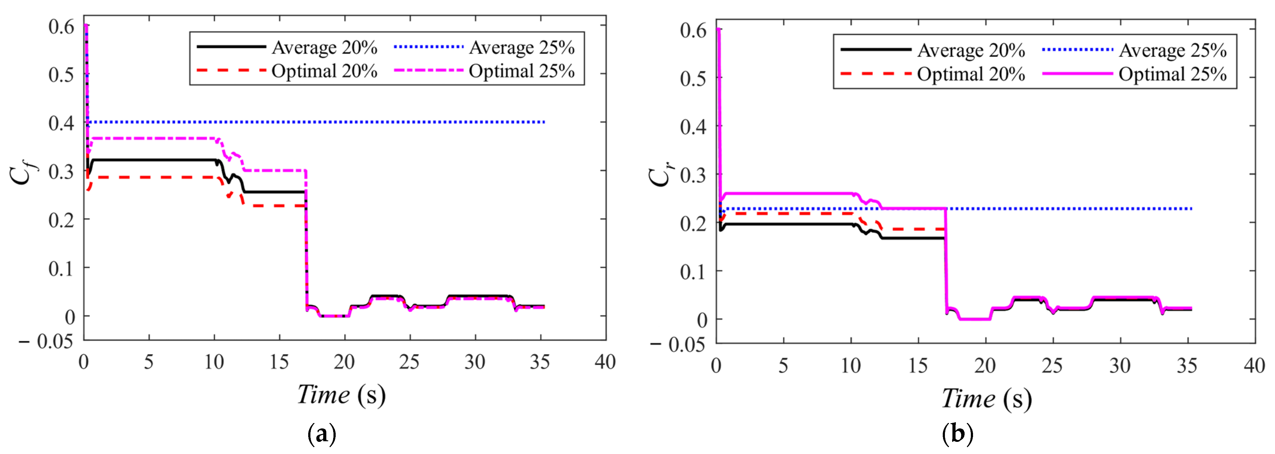
5.3. Optimal Driving Torque Distribution Simulation

The driving torque distribution algorithm simulation compares the driving torque and tire adhesion utilization rate of the four wheels between the optimal distribution and the average distribution, as the comparative strategy adopted in [35]. The driving torque and adhesion utilization rate of the AGV’s four wheels are shown in Figure 12, and the maximum adhesion utilization rates on different road sections are listed in Table 5.
At the beginning of the simulation, the AGV starts from static and needs more drive torque to overcoming static friction including tire–road friction, the wheel moment of inertia, and gear resistance, leading to the maximum adhesion utilization rate of 0.6. During the climbing straight section, significant vertical load transfer to the rear wheels occurs, resulting in 12.52% higher driving torque at the rear wheels compared to the front wheels. In this scenario, the driving torque optimal distribution algorithm significantly reduces the maximum adhesion utilization rate compared to the average distribution algorithm. In the curve sections, due to the low acceleration and speed of the AGV, the vertical load transfer of the tires is not significant, and the reduction in the maximum adhesion utilization rate is minimal compared to the average distribution algorithm.
Simulation results demonstrate that the optimal torque distribution strategy significantly reduces the peak tire–road friction utilization rate in the front wheels during climbing, which is caused by longitudinal load transfer in factory test scenarios. By optimizing vertical load utilization, the algorithm provides greater lateral force margin to prevent wheel slip. To further investigate its anti-slip performance, tests were conducted on a wet factory road (with an adhesion coefficient of 0.4) with 20% and 25% gradient while maintaining the above trajectories [42]. Figure 13 presents the tire adhesion utilization rate during these conditions.
The results reveal that the low speed of the AGV reduces adhesion utilization rate variations in the Curve 1 and Curve 2 sections despite the slippery conditions. However, significant load transfer during climbing causes notable adhesion utilization rate differences between the front and rear wheels, with the front wheels consistently exhibiting higher values and slip risks. At the 20% gradient, the optimal strategy reduces tire adhesion utilization rate by 11.12% compared to average distribution. At the 25% gradient, average distribution causes front wheel slip (demanded adhesion coefficient > 0.4), preventing climb completion. The optimal strategy exploits the adhesion of the front wheels while increasing the driving force of the rear wheels, successfully completing the climb under the adhesion coefficient limit and maintaining path-tracking capability, thereby enhancing the AGV’s gradeability.

6. Conclusions

To address the issues of lateral instability and wheel slippage during acceleration, climbing and turning for four-steering-wheel heavy-duty AGVs, an IMPC trajectory tracking strategy considering lateral stability and an optimal driving torque distribution strategy accounting for load transfer and the tire adhesion coefficient are proposed. Based on steering angles, different motion modes were selected, and the sideslip angle was incorporated into the cost function to develop the IMPC trajectory tracking strategy. Compared with conventional MPC algorithms, the proposed IMPC strategy reduces the sideslip angle by 58.18% while maintaining trajectory tracking accuracy. Furthermore, the effects of longitudinal/lateral acceleration and road gradient on vertical load transfer were analyzed. By fully utilizing differences in maximum adhesion forces across wheels, a quadratic programming-based driving torque distribution method was implemented. Compared to average distribution strategies, the optimal distribution approach reduces the maximum wheel adhesion utilization rate by 6.62% during climbing operations and improves climbing gradeability on wet road surfaces, thereby enhancing the overall control margin and reducing the risk of wheel slippage.

Author Contributions

Conceptualization, X.L.; Data Curation, B.L.; Investigation, X.C.; Methodology, X.L. and X.C.; Project Administration, X.L. and C.W.; Software, X.C.; Supervision, X.L.; Validation, X.L., X.C. and S.C.; Visualization, S.C. and C.W.; Writing—Original Draft, X.L., X.C. and C.W.; Writing—Review and Editing, X.C. and B.L. All authors have read and agreed to the published version of the manuscript.

Funding

This research received no external funding.

Data Availability Statement

The original contributions presented in this study are included in the article. Further inquiries can be directed to the corresponding author.

Conflicts of Interest

The authors declare no conflicts of interest.

References

  1. Gupta, M.K. Review on Optimization Techniques for AGV’s Optimization in Flexible Manufacturing System. Gazi U. J. Sci. 2023, 36, 399–412. [Google Scholar] [CrossRef]
  2. Zhang, W.; Drugge, L.; Nybacka, M.; Jerrelind, J.; Wang, Z. Exploring Four-Wheel Steering for Trajectory Tracking of Autonomous Vehicles in Critical Conditions. In Proceedings of the IAVSD International Symposium on Dynamics of Vehicles on Roads and Tracks, Ottawa, ON, Canada, 21–25 August 2023. [Google Scholar]
  3. Ran, Q.; Yao, S.; Chen, X.; Bi, G. Trajectory Tracking of Swing-Arm Type Omnidirectional Mobile Robot. Math. Probl. Eng. 2022, 2022, 3297789. [Google Scholar] [CrossRef]
  4. Hang, P.; Chen, X. Towards Autonomous Driving: Review and Perspectives on Configuration and Control of Four-Wheel Independent Drive/Steering Electric Vehicles. Actuators 2021, 10, 184. [Google Scholar] [CrossRef]
  5. Wang, B.; Fan, G.; Zhang, X.; Gao, L.; Wang, X.; Fu, W. Multistep Prediction Analysis of Pure Pursuit Method for Automated Guided Vehicles in Aircraft Industry. Actuators 2024, 13, 518. [Google Scholar] [CrossRef]
  6. Mahdi, M.T.; Nadour, M.; Cherroun, L.; Kouzou, A. Robust and Intelligent Fuzzy Logic Controllers for a Differential Mobile Robot Trajectory Tracking. In Proceedings of the International Conference on Artificial Intelligence and Its Applications in the Age of Digital Transformation, Nouakchott, Mauritania, 23–25 April 2024. [Google Scholar]
  7. Kati, M.S.; Jonas, F.; Bengt, J.; Laine, L. A Feedback-Feed-Forward Steering Control Strategy for Improving Lateral Dynamics Stability of an A-Double Vehicle at High Speeds. Veh. Syst. Dyn. 2022, 60, 3955–3976. [Google Scholar] [CrossRef]
  8. He, M.; Ji, P.; Ma, F. Research on Path Tracking Algorithm of Differential Drive Robots Based on Lookahead Distance Adaptive. In Proceedings of the Ninth International Symposium on Advances in Electrical, Electronics, and Computer Engineering (ISAEECE 2024) ISAEECE 2024, Changchun, China, 15–17 March 2024. [Google Scholar]
  9. Sun, Q.; Li, M.; Cheng, J.; Wang, Z.; Liu, B.; Tai, J. Path Tracking Control of Wheeled Mobile Robot Based on Improved Pure Pursuit Algorithm. In Proceedings of the Chinese Automation Congress (CAC), Hangzhou, China, 22 November 2019. [Google Scholar]
  10. Wang, M.; Lv, X.; Chen, J.; Su, X. Improved Pure Pursuit Algorithm Based Path Tracking Method for Autonomous Vehicle. J. Adv. Comput. Intell. Inform. 2024, 28, 1034–1042. [Google Scholar] [CrossRef]
  11. Ahn, J.; Shin, S.; Kim, M.; Park, J. Accurate Path Tracking by Adjusting Look-Ahead Point in Pure Pursuit Method. Int. J. Automot. Technol. 2021, 22, 119–129. [Google Scholar] [CrossRef]
  12. Wang, X.; Xu, B.; Guo, Y. Fuzzy Logic System-Based Robust Adaptive Control of AUV with Target Tracking. Int. J. Fuzzy Syst. 2023, 25, 338–346. [Google Scholar] [CrossRef]
  13. Ryoo, Y.-J. Trajectory-Tracking Control of a Transport Robot for Smart Logistics Using the Fuzzy Controller. Int. J. Fuzzy Log. Intell. Syst. 2022, 22, 69–77. [Google Scholar] [CrossRef]
  14. Zhang, C.; Gao, G.; Zhao, C.; Li, L.; Li, C.; Chen, X. Research on 4WS Agricultural Machine Path Tracking Algorithm Based on Fuzzy Control Pure Tracking Model. Machines 2022, 10, 597. [Google Scholar] [CrossRef]
  15. Wang, Y.; Jiang, B.; Wu, Z.-G.; Xie, S.; Peng, Y. Adaptive Sliding Mode Fault-Tolerant Fuzzy Tracking Control with Application to Unmanned Marine Vehicles. IEEE Trans. Syst. Man Cybern. Syst. 2021, 51, 6691–6700. [Google Scholar] [CrossRef]
  16. Nguyen, A.-T.; Rath, J.; Guerra, T.-M.; Palhares, R.; Zhang, H. Robust Set-Invariance Based Fuzzy Output Tracking Control for Vehicle Autonomous Driving under Uncertain Lateral Forces and Steering Constraints. IEEE Trans. Intell. Transp. Syst. 2021, 22, 5849–5860. [Google Scholar] [CrossRef]
  17. Viadero-Monasterio, F.; Nguyen, A.-T.; Lauber, J.; Boada, M.J.L.; Boada, B.L. Event-Triggered Robust Path Tracking Control Considering Roll Stability under Network-Induced Delays for Autonomous Vehicles. IEEE Trans. Intell. Transp. Syst. 2023, 24, 14743–14756. [Google Scholar] [CrossRef]
  18. Chen, C.; Shu, M.; Yang, Y.; Gao, T.; Bian, L. Robust H∞ Path Tracking Control of Autonomous Vehicles with Delay and Actuator Saturation. J. Control Decis. 2022, 9, 45–57. [Google Scholar] [CrossRef]
  19. Kennouche, A.; Saifia, D.; Chadli, M.; Labiod, S. Multi-Objective H2/HSaturated Non-PDC Static Output Feedback Control for Path Tracking of Autonomous Vehicle. Trans. Inst. Meas. Control 2022, 44, 2235–2247. [Google Scholar] [CrossRef]
  20. Chen, Y.; Gai, J.; He, S.; Li, H.; Cheng, C.; Zou, W. MPC-TD3 Trajectory Tracking Control for Electrically Driven Unmanned Tracked Vehicles. Electronics 2024, 13, 3747. [Google Scholar] [CrossRef]
  21. Tang, M.; Lin, S.; Luo, Y. Mecanum Wheel AGV Trajectory Tracking Control Based on Efficient MPC Algorithm. IEEE Access 2024, 12, 13763–13772. [Google Scholar] [CrossRef]
  22. Xu, Y.; Tang, W.; Chen, B.; Qiu, L.; Yang, R. A Model Predictive Control with Preview-Follower Theory Algorithm for Trajectory Tracking Control in Autonomous Vehicles. Symmetry 2021, 13, 381. [Google Scholar] [CrossRef]
  23. Leman, Z.A.; Ariff, M.H.M.; Zamzuri, H.; Rahman, M.A.A.; Mazlan, S.A.; Bahiuddin, I.; Yakub, F. Adaptive Model Predictive Controller for Trajectory Tracking and Obstacle Avoidance on Autonomous Vehicle. J. Teknol. (Sci. Eng.) 2022, 84, 139–148. [Google Scholar]
  24. Li, Y.; He, D.; Ma, F.; Liu, P.; Liu, Y. MPC-Based Trajectory Tracking Control of Unmanned Underwater Tracked Bulldozer Considering Track Slipping and Motion Smoothing. Ocean Eng. 2023, 279, 114449. [Google Scholar] [CrossRef]
  25. Viadero-Monasterio, F.; García, J.; Meléndez-Useros, M.; Jiménez-Salas, M.; Boada, B.L.; López Boada, M.J. Simultaneous Estimation of Vehicle Sideslip and Roll Angles Using an Event-Triggered-Based IoT Architecture. Machines 2024, 12, 53. [Google Scholar] [CrossRef]
  26. Chen, B.-S.; Wu, P.-H. Robust H∞ Observer-Based Reference Tracking Control Design of Nonlinear Stochastic Systems: HJIE-Embedded Deep Learning Approach. IEEE Access 2022, 10, 39889–39911. [Google Scholar] [CrossRef]
  27. Yoon, K.; Choi, J.; Huh, K. Adaptive Decentralized Sensor Fusion for Autonomous Vehicle: Estimating the Position of Surrounding Vehicles. IEEE Access 2023, 11, 90999–91008. [Google Scholar] [CrossRef]
  28. Zhai, L.; Sun, T.; Wang, J. Electronic Stability Control Based on Motor Driving and Braking Torque Distribution for a Four In-Wheel Motor Drive Electric Vehicle. IEEE Trans. Veh. Technol. 2016, 65, 4726–4739. [Google Scholar] [CrossRef]
  29. Wu, X.; Zheng, D.; Wang, T.; Du, J. Torque Optimal Allocation Strategy of All-Wheel Drive Electric Vehicle Based on Difference of Efficiency Characteristics between Axis Motors. Energies 2019, 12, 1122. [Google Scholar] [CrossRef]
  30. Zhou, H.; Lu, Z.; Deng, X.; Zhang, C.; Luo, G.; Zhou, R. Study on Torque Distribution of Traction Operation of Four Wheel Independent Driven Electric Tractor. J. Nanjing Agric. Univ. 2018, 41, 962–970. [Google Scholar]
  31. Zhang, X.; Wang, B.; Deng, Z.; Wu, H.; Zhu, Y. Research on Stability of Four-Wheel Independent Electric Drive Vehicle Based on Sliding Mode Coordinated Control. Mod. Manuf. Eng. 2024, 1, 51–57. [Google Scholar] [CrossRef]
  32. Rahmanei, H.; Aliabadi, A.; Ghaffari, A.; Azadi, S. Lyapunov-Based Control System Design for Trajectory Tracking in Electrical Autonomous Vehicles with in-Wheel Motors. J. Frankl. Inst.-Eng. Appl. Math. 2024, 361, 106736. [Google Scholar] [CrossRef]
  33. Li, W.; Zhang, Y.; Qin, Y.; Zhao, F.; Wan, M.; Gao, F. Research on Multi-Objective Optimization Torque Distribution Strategy for Distributed Drive Electric Vehicles Based on Dung Beetle Optimizer. Phys. Scr. 2025, 100, 015252. [Google Scholar] [CrossRef]
  34. Cao, K.; Hu, M.; Wang, D.; Qiao, S.; Guo, C.; Fu, C.; Zhou, A. All-Wheel-Drive Torque Distribution Strategy for Electric Vehicle Optimal Efficiency Considering Tire Slip. IEEE Access 2021, 9, 25245–25257. [Google Scholar] [CrossRef]
  35. Morera-Torres, E.; Ocampo-Martinez, C.; Bianchi, F.D. Experimental Modelling and Optimal Torque Vectoring Control for 4WD Vehicles. IEEE Trans. Veh. Technol. 2022, 71, 4922–4932. [Google Scholar] [CrossRef]
  36. Liu, W.; Liu, P.; Yu, Y.; Zhang, Q.; Wan, Y.; Wang, M. Optimal Torque Distribution of Distributed Driving AGV under the Condition of Centroid Change. Sci. Rep. 2021, 11, 21404. [Google Scholar] [CrossRef] [PubMed]
  37. Kim, H.-W.; Amarnathvarma, A.; Kim, E.; Hwang, M.-H.; Kim, K.; Kim, H.; Choi, I.; Cha, H.-R. A Novel Torque Matching Strategy for Dual Motor-Based All-Wheel-Driving Electric Vehicles. Energies 2022, 15, 2717. [Google Scholar] [CrossRef]
  38. Siwek, M.; Panasiuk, J.; Baranowski, L.; Kaczmarek, W.; Prusaczyk, P.; Borys, S. Identification of Differential Drive Robot Dynamic Model Parameters. Materials 2023, 16, 683. [Google Scholar] [CrossRef]
  39. Zhang, Y.; Wang, Z.; Wang, Y.; Zhang, C.; Zhao, B. Research on Automobile Four-Wheel Steering Control System Based on Yaw Angular Velocity and Centroid Cornering Angle. Meas. Control 2022, 55, 49–61. [Google Scholar] [CrossRef]
  40. Cao, G.; Zhao, X.; Ye, C.; Yu, S.; Li, B.; Jiang, C. Fuzzy Adaptive PID Control Method for Multi-Mecanum-Wheeled Mobile Robot. J. Mech. Sci. Technol. 2022, 36, 2019–2029. [Google Scholar] [CrossRef]
  41. Doroliat, A.P.; Ing, M.-H.; Li, C.-H.G. Optimization of Mecanum Wheels for Mitigation of AGV Vibration. Int. J. Adv. Manuf. Technol. 2022, 121, 633–645. [Google Scholar] [CrossRef]
  42. Yu, Z.; Xia, Q. Automobile Theory, 6th ed.; China Machine Press: Beijing, China, 2018; pp. 9–24. [Google Scholar]
Figure 1. Structure of four-steering-wheel heavy-duty AGV. 1—Laser radar; 2—Load-bearing plate; 3—Steering wheel; 4—Controller; 5—Battery.
Machines 13 00383 g001
Figure 2. Structure of steering wheel module. 1—Drive motor; 2—Steering gear; 3—Drive wheel; 4—Hydraulic absorber; 5—Steer motor.
Machines 13 00383 g002
Figure 3. AGV straight-line motion. (a) Forward. (b) Diagonal. (c) Lateral.
Machines 13 00383 g003
Figure 4. AGV curve motion. (a) Single Ackermann steering. (b) Double Ackermann steering.
Machines 13 00383 g004
Figure 5. AGV pivot steering.
Machines 13 00383 g005
Figure 6. The 3DOF four-steering-wheel AGV motion model.
Machines 13 00383 g006
Figure 7. Dynamic model of four-steering-wheel heavy-duty AGV.
Machines 13 00383 g007
Figure 8. Vertical load transfer model of four-steering-wheel heavy-duty AGV.
Machines 13 00383 g008
Figure 9. Co-simulation model of trajectory tracking and driving torque distribution.
Machines 13 00383 g009
Figure 10. Simulation road for trajectory tracking and driving torque distribution.
Machines 13 00383 g010
Figure 11. Trajectory tracking simulation of four-steering-wheel AGV. (a) AGV trajectory on simulation road. (b) Steering angles of four wheels under IMPC strategy. (c) Steering angles of four wheels under MPC strategy. (d) Sideslip angle of centroid under IMPC and MPC strategy.
Machines 13 00383 g011
Figure 12. Driving torque distribution simulation of four-steering-wheel AGV. (a) Driving torque of four wheels. (b) Adhesion utilization rate of front left wheel. (c) Adhesion utilization rate of front right wheel. (d) Adhesion utilization rate of rear left wheel. (e) Adhesion utilization rate of rear right wheel.
Machines 13 00383 g012
Figure 13. Adhesion utilization rate of wheels on wet factory road. (a) Adhesion utilization rate of front wheels. (b) Adhesion utilization rate of rear wheels.
Machines 13 00383 g013
Table 1. Parameters of four-steering-wheel heavy-duty AGV.
ParameterUnitValue
curb qualityt2
gross qualityt7
minimum turning radiusm0
maximum speedm/s2
maximum accelerationm/s20.2
vehicle size (length × width × height)mm5000 × 1800 × 900
cargo stacking heightmm1200
Table 2. ADAMS AGV model parameters.
ParameterUnitValue
total masst7
moment of inertiakg·m25099
wheelbasemm3780
wheel trackmm1240
height of the center of massmm1100
driving wheel radiusmm300
tire cornering stiffnessN/rad−40,000
tire–road adhesion coefficient 0.7
tire–road rolling resistance coefficient 0.02
Table 3. Simulation road parameters.
ParameterUnitValue
straight section lengthm20
straight section widthm5
straight section gradient 10%
curve 1 centerline radiusm5
curve 1 widthm5
curve 2 centerline radiusm10
curve 2 widthm10
Table 4. Tracking errors for reference path.
Road SectionMotion ModesMax Steady-State Error
starting pointstart from static0.5 m
climbing straightdouble Ackermann0.0189 m
curve 1diagonal0.0195 m
curve 2double Ackermann0.0443 m
Table 5. Simulation results of maximum adhesion utilization rate.
Road SectionAverage DistributionOptimal DistributionReduction Percentage
climbing straight0.1510.1416.62%
curve 10.04210.04112.4%
curve 20.03980.03872.26%
Disclaimer/Publisher’s Note: The statements, opinions and data contained in all publications are solely those of the individual author(s) and contributor(s) and not of MDPI and/or the editor(s). MDPI and/or the editor(s) disclaim responsibility for any injury to people or property resulting from any ideas, methods, instructions or products referred to in the content.

