Nonlinear Vibration Analysis of Turbocharger Rotor Supported on Rolling Bearing by Modified Incremental Harmonic Balance Method

Abstract

High-speed rolling bearings exhibit low friction, high mechanical efficiency, low lubrication requirements, and excellent acceleration performance. The replacement of floating ring bearings in turbochargers with rolling bearings is an important tendency for modern turbochargers. However, due to the nonlinearity in rolling bearings, the nonlinear vibration characteristics of the turbocharger rotor system need to be clearly revealed. The turbocharger rotor is modeled by a lumped mass model. The nonlinear rolling bearing model is derived using the Hertz contact theory. The vibration responses of the nonlinear system are obtained by the modified incremental harmonic balance (MIHB) method. The results demonstrate that the MIHB method significantly improves computational efficiency compared to the traditional fourth-order Runge–Kutta method for solving this class of problems while also being capable of obtaining complete solution branches of the system. The stability of the responses is determined by the Floquet theory. Based on the present rotor dynamic model, the conical mode and cylindrical mode are found. Resonance peaks at 4.5 × 10⁴ rpm (conical mode) and 1.1 × 10⁵ rpm (bending mode) are identified as critical vibration thresholds. Moreover, the vibration amplitude results show that the resonance peak of the bending mode is mainly due to the nonlinearity of the rolling bearings, which also causes the amplitude jumping phenomenon. Changing the parameters of the rolling bearing could avoid the resonance peak appearing in the working speed range. The amplitude of the system under different rotating speeds could be suppressed by choosing the appropriate parameters of the rolling bearing.

1. Introduction

A turbocharger is a type of air compressor that increases the intake volume by compressing air. It can enhance the engine’s output power [1,2]. Turbochargers are widely utilized in automotive engines, agricultural machinery, aircraft engines, and other fields. They represent a typical rotor-bearing system [3]. Turbocharger rotors are commonly supported on floating ring bearings. It has excellent damping capability, almost infinite service life, and is cheaper than rolling bearings [4]. However, it is subjected to considerable sub-synchronous vibrations when one or both oil films become unstable [5,6]. Meanwhile, high-speed rolling bearings exhibit low friction, high mechanical efficiency, low lubrication requirements, and excellent acceleration performance [7]. Rolling bearings have become popular as a replacement for floating ring bearings in turbochargers. However, research on the nonlinear dynamics of turbochargers supported by rolling bearings is still quite limited.

When applying rolling bearings to turbocharger rotors, as the balls periodically transition from the loaded area to the unloaded area, the stiffness of the bearing varies, and the vibration induced by this varying stiffness is an inevitable source of excitation to the rotor bearing system [8,9]. The system may possess complex dynamic properties caused by the coupled nonlinearities among bearing clearance and Hertz contact between the balls and cage. Rolling bearings can introduce a significant amount of nonlinear phenomena, such as bistability, into the system due to its intrinsic nonlinearity [10]. The bistable behavior can cause a jump of amplitude in the turbocharger system when the rotating speed changes, which is an impact source that the system needs to suppress [11,12,13]. Based on early research, the impact effect is an important factor in shortening the life of bearing components [14].

Many scholars have attempted to analyze the dynamics of rotor systems in depth in recent years. Andres et al. [15,16,17] constructed a comprehensive model for predicting the dynamic characteristics of turbocharger systems. It presented a perspective to find out the dynamic effects of bearings in turbochargers. Bonello [18] constructed a nonlinear model to study the dynamics of turbochargers on full-floating and semi-floating ring bearings. Tian et al. [19,20,21] studied the dynamic response and synchronous and sub-synchronous vibrations of turbocharger rotor systems supported on floating ring bearings. Ouyang et al. [22] investigated the effect of weight on the critical speed of an inclined turbocharger rotor coupled with floating ring bearings. Kong et al. [23] presented the reliability of the rotor-bearing system of an EAT supported by floating ring bearings under strong impact. These studies mostly focused on investigating turbochargers supported by floating-ring bearings. Mutra et al. [24] conducted dynamic analysis and active vibration control research on practical turbocharger rotor systems utilizing electromagnetic actuator (EMA) systems. The modeling in these research studies is, to some extent, applicable to turbochargers supported by rolling bearings [25]. Ghaisas et al. [26] constructed a six-degree-of-freedom, fully dynamic discrete element model that considered bearing components as sections of spheres and cylinders, and it significantly reduced the computational effort associated with bearing dynamic modeling. In recent years, the robust design of rotor systems has garnered significant attention, with parameter uncertainty quantification methods such as Monte Carlo simulation and interval analysis demonstrating substantial application potential. Zhao et al. [27] gave a comprehensive review of dimensional decomposition-aided metamodels for high-dimensional uncertainty quantification and optimization in engineering. Mofid et al. [28] proposed an adaptive regulation strategy to maintain stability and trajectory tracking performance for aerial rotating machinery subject to parameter variations. Fu et al. [29] developed finite element modeling and deterministic solutions for aero-engine dual-rotor systems. Subsequently, under non-random uncertainty conditions, they constructed polynomial surrogate functions for required natural characteristics and dynamic responses. The polar coordinate interpolation technique was employed to compute uncertain shaft orbits, overcoming the limitations of traditional frequency-response measurement methods. Ashtekar et al. [30] established a combined model of rolling bearings and squeeze film dampers and solved the dynamic response of the turbocharger by coupling this combined model with traditional quasi-static models and time-dependent rotor dynamic models. Chang et al. [31] combined lumped parameters with a thermal network to establish a heat transfer model for ball bearings that considers the frictional heat caused by dynamic loads on the bearings. They coupled the heat transfer model with the motion equation of the rotor system through the mechanical model of ball bearings and the dynamic, and thermal bidirectional coupling model of the rotor was solved using a step-by-step iterative solution procedure. However, these researchers typically use numerical methods, such as the R-K method, to obtain the solution of the rotor system. Traditional numerical methods only reflect the gradual characteristics of the system in the time domain. For low-damping systems, it takes a long time for the system to reach a steady-state response, and the calculation of the response is time-consuming. Moreover, the initial value problem method cannot obtain unstable solutions for the system, making it difficult to track the rotating speed range where bistable behavior appears [32].

Derived from the classical harmonic balance method, the incremental harmonic balance method (IHB) has overcome the limitations of traditional analytical methods like perturbation and averaging methods, which rely on small parameters and are less accurate for strongly nonlinear problems [33,34,35]. This IHB method has been widely applied in rotor systems equipped with either rolling bearings or squeeze film dampers [36,37]. Ju et al. [38] presented a modified incremental harmonic balance (MIHB) method by tensor contraction and fast Fourier transform (FFT) to efficiently calculate the residual vector and Jacobian matrix. This method shows good consistency with traditional numerical methods in the coupled thermo-mechanical model of a rotor-ball bearing system [39,40]. Chen [41,42] promoted a more efficient MIHB to solve the nonlinear vibrations of dual-rotor systems. When applying the MIHB method to solve system equations, it is often necessary to calculate the linear Jacobian matrix, i.e., the equivalent stiffness and damping. In large mechanical networks, determining these equivalent parameters proves particularly challenging and computationally inefficient. Yang et al. [43] proposed a frequency-dependent equivalent impedance (FDEI)-based approach for analyzing the dynamic characteristics of mechanical networks. This method replaces lumped masses with inerter units to construct mechanical networks, offering a novel perspective for computing system equivalent stiffness and damping. Zhou et al. [44] proposed a finite element modeling method for rotor-bearing systems with bolted flange joints to analyze their nonlinear vibration characteristics and developed an incremental harmonic balance method incorporating arc-length continuation to solve the dynamic responses of the rotor system.

Currently, there is still a lack of research on applying the MIHB method to the coupling of turbocharged rotor systems with rolling bearings.

The motivation of this paper is to extend the MIHB method to reveal the nonlinear vibration of the turbocharger rotor system coupled with the rolling bearing under different rotating speeds. The MIHB method embedding arc-length continuation is applied to obtain the periodic responses, and the stability of the responses is determined by the Floquet theory. Then, the vibration modes of the rotor system are obtained. Lastly, the influences of different parameters of the rotor and rolling bearing on the vibration amplitude are discussed in detail.

2. Rolling Bearing-Supported Turbocharger Rotor Model

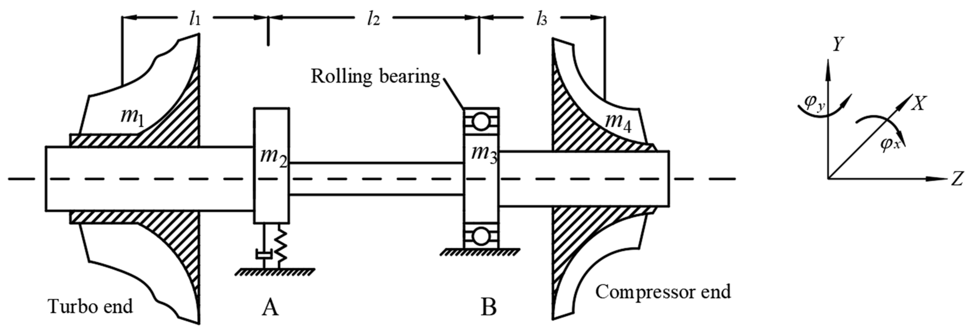
2.1. Dynamic Model of Rotor System

The schematic diagram of the rolling bearing-supported turbocharger rotor model is shown in Figure 1. To meet the system’s damping requirements, the rotor is supported by one rolling bearing and one graphite-lubricated bearing, where the graphite-lubricated bearing can be simplified as a linear stiffness k_c and a linear damping c_n. C_b in the figure represents the Hertz contact stiffness of the rolling bearing, and ω represents the rotating speed. The rotor system consists of two disks (turbine end and compressor end), rolling bearings, elastic support, and the shaft. According to the lumped mass method [22,23], the system can be simplified to four lumped masses, where m₁ and m₄, respectively, represent the mass at the turbine end and the mass at the compressor end, and m₂ and m₃, respectively, represent the lumped mass at the graphite-lubricated bearing constraint and rolling bearing constraint. Assuming that the mass of the shaft is distributed on the rigid disk, there are no individual degrees of freedom for the shaft. l₁, l₂, and l₃ are the lengths of the three axes connecting four lumped masses. Bearing A is a graphite lubricated bearing, and bearing B is a rolling bearing. On the turbocharger rotor, thrust bearings are installed to withstand the axial thrust generated by the rotor and limit its axial displacement. Therefore, axial vibration is not considered, and torsional vibration and shear effects of the rotor are ignored. Due to the cantilever characteristics of the rotor wheel, the degrees of freedom of the wheel disc’s rotation angle and gyroscopic effects cannot be ignored. φ_x and φ_y are the angles of lumped mass around the x-axis and y-axis, respectively [45,46].

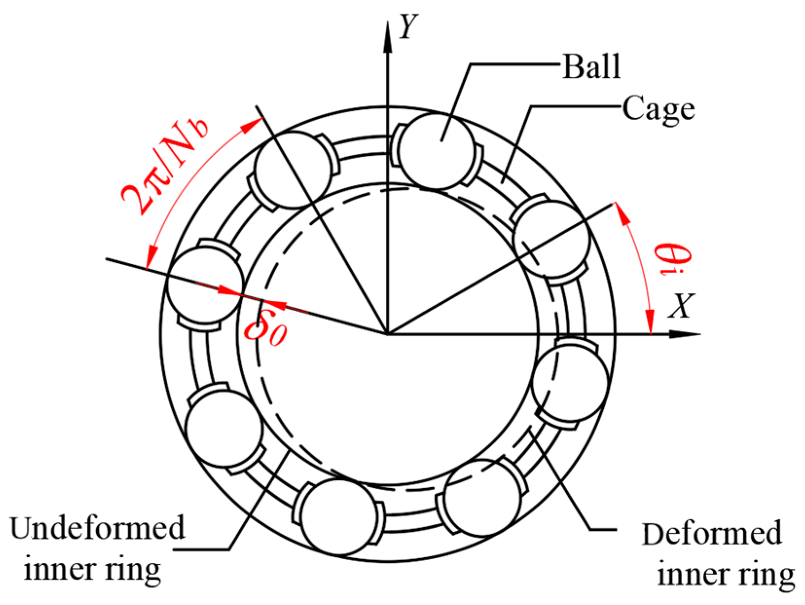
2.2. Dynamic Model of Rolling Bearings

The ball bearing is the source of the nonlinearities of the system, the outer ring is fixed on the rigid bearing housing, and the rolling elements do pure rolling between the inner ring and the outer ring. Then, the rotating speed of the cage can be expressed as

$$\Omega ={\displaystyle \frac{d_i{\omega }_i+d_o{\omega }_o}{d_i+d_o}}$$

(1)

where ω_i = ω is the rotating speed of the inner ring. d_i and d_o are the diameters of the inner and outer ring, respectively. Figure 2 displays the schematic diagram of the ball bearing.

The elastic deformation between the ith (i = 1, 2,…, N_b) ball and rings is expressed as

$${\delta }_i=X_3\cos {\theta }_i+Y_3\sin {\theta }_i-{\delta }_0$$

(2)

where δ₀ is the initial radial clearance, and X₃ and Y₃ represent the horizontal and vertical displacements of the lumped mass 3 corresponding to the rolling bearing, respectively. The angle at which the ith ball rotates is given as

$${\theta }_i=2\pi (i-1)/N_b+\Omega t$$

(3)

The vertical and horizontal elastic restoring forces of the rolling bearing are [47]

$$\left[\begin{array}{l}{F}_{\delta x3}\\ F_{\delta y3}\end{array}\right]=C_b{{\displaystyle \sum _{i=1}^{N_b}({\delta }_{i}G[{\delta }_i])}}^{{\displaystyle \frac{3}{2}}}\left[\begin{array}{l}\cos {\theta }_i\\ \sin {\theta }_i\end{array}\right]$$

(4)

where $G(x)=\left\{\begin{array}{l}1(x>0)\\ 0(x\le 0)\end{array}\right.$ represents the Heaviside function.

2.3. Dynamic Model of the Rotor-Rolling Bearing System

Following the method given in Refs. [22,23], the governing equations of motion for the turbocharger rotor system can be derived as follows:

$$\mathbf{M}\ddot{\mathit{q}}+(\omega \mathbf{G}+\mathbf{C})\dot{\mathit{q}}+\mathbf{K}\mathit{q}=-{\mathit{F}}_{\delta }+{\mathit{F}}_{ub}+{\mathit{F}}_g$$

(5)

where q = {X₁, φ_y1, X₂, φ_y2, X₃, φ_y3, X₄, φ_y4, Y₁, φ_x1, Y₂, φ_x2, Y₃, φ_x3, Y₄, φ_x4}^T is the system displacement vector, M is the mass matrix, G is the matrix caused by gyroscopic effect, K is the stiffness matrix, where K₁ is the structural stiffness matrix, and K₂ is the equivalent stiffness matrix of the graphite-lubricated bearing. F_ub is the unbalanced force caused by eccentricity at the compressor and turbine ends, and F_g is gravity. The detailed expressions of these matrices can be found in Refs. [22,23]. Moreover, C is the damping matrix, which includes the Rayleigh damping matrix (C₁) and the damping matrix of the graphite-lubricated bearing (C₂).

$$\mathbf{K}={\mathbf{K}}_1+{\mathbf{K}}_2$$

(6)

$${\mathbf{K}}_2=\mathrm{diag}\left[\begin{array}{cccccccccccccccc}0& 0& k_c& 0& 0& 0& 0& 0& 0& 0& k_c& 0& 0& 0& 0& 0\end{array}\right]$$

(7)

$$\mathbf{C}={\mathbf{C}}_1+{\mathbf{C}}_2,{\mathbf{C}}_1={\alpha }_1\mathbf{M}+{\beta }_1\mathbf{K}$$

(8)

$${\mathbf{C}}_2=\mathrm{diag}\left[\begin{array}{cccccccccccccccc}0& 0& c_n& 0& 0& 0& 0& 0& 0& 0& c_n& 0& 0& 0& 0& 0\end{array}\right]$$

(9)

in which ${\alpha }_1={\displaystyle \frac{4\pi f_1{f}_2(f_2{\xi }_1-f_1{\xi }_2)}{f_2^2-f_1^2}}$, ${\beta }_1={\displaystyle \frac{f_2{\xi }_2-f_1{\xi }_1}{\pi (f_2^2-f_1^2)}}$ [48], f₁, and f₂ are the first- and second-order natural frequencies of the system. ξ₁ and ξ₂ are the first= and second-order modal damping ratios of the system.

3. The MIHB Method for Nonlinear Dynamic Analysis

The most widely used method for solving this type of rotor model is the Runge–Kutta method. It fails to work well when dynamic systems have multiple solutions because it depends a lot on the initial guess, and it consumes a lot of time to reach a steady-state response. In order to obtain a complete solution branch of the system, the IHB method is widely used. However, when the IHB method is used for a system with non-polynomial nonlinearities, numerical integration is needed in the Galerkin averaging procedure to obtain residual vector and Jacobian matrix, which will result in extremely low solving efficiency. Thus, in this case, it is necessary to apply an MIHB method, which is able to calculate the residual vector and Jacobian matrix by introducing the tensor contraction and FFT. The displacement of each degree of freedom and nonlinear forces can be expanded into time-varying trigonometric basis vectors related to nonlinear terms and series coefficients. Complete periodic solution branches can be obtained by embedding arc-length continuation. Moreover, the Floquet theory is adopted to analyze the stability of periodic solutions. The detailed method is given in the following.

3.1. IHB Method Based on Tensor Contraction and FFT

Substituting dimensionless time τ = ωt into Equation (5), the dynamic equations of the rotor and rolling bearing system can be rewritten as

$${\omega }^2\mathbf{M}{\mathit{q}}^{″}+(\omega \mathbf{G}+\mathbf{C})\omega {\mathit{q}}^{\prime }+\mathbf{K}\mathit{q}=-{\mathit{F}}_{\delta }+{\mathit{F}}_{ub}+{\mathit{F}}_g$$

(10)

where “ ′ ” and “ ″ ” represent the first and second derivatives of q with respect to τ, respectively. In Equation (5), F_ub, q are vectors related to τ, and F_δ is a vector related to τ and q. The degree of freedom of the system is 16. q can be expanded based on degrees of freedom as

$$\mathit{q}={\left\{\begin{array}{ccccc}{q}_1& q_2& q_3& \cdots & q_{16}\end{array}\right\}}^{\mathrm{T}}$$

(11)

According to the harmonic balance method, the displacement of the kth degree of freedom q_k(τ) can be expressed in the form of Fourier series as

$$q_k(\tau )=a_{k,0}+{\displaystyle \sum _{u=1}^h(a_{k,u}\cos u\tau +b_{k,u}\sin }u\tau )(k=1,2,\dots ,16)$$

(12)

where h is the number of truncated harmonic terms of the periodic solution, and h is decided by the vibration characteristics of the system [49].

The solution vector q can also be expressed in the form of a Fourier series as

$$\mathit{q}={\mathbf{U}}_0\mathit{Y} {\mathit{q}}^{\prime }={\mathbf{U}}_0^{\prime }\mathit{Y} {\mathit{q}}^{″}={\mathbf{U}}_0^{″}\mathit{Y}$$

(13)

where U₀ is the basis of a series.

$$U_0={\left[\begin{array}{ccccc}\mathit{B}& & & & \\ & \ddots & & & \\ & & \mathit{B}& & \\ & & & \ddots & \\ & & & & \mathit{B}\end{array}\right]}_{16\times [16\times (2h+1)]}$$

(14)

$$\mathit{B}=\left\{\begin{array}{ccccccccc}1\hfill & \cos \tau \hfill & \cos 2\tau \hfill & \cdots \hfill & \cos h\tau \hfill & \sin \tau \hfill & \sin 2\tau \hfill & \cdots \hfill & \sin h\tau \hfill \end{array}\right\}$$

(15)

And Y is the coefficient vector. It can be written as

$$\mathit{Y}={\left\{\begin{array}{cccc}{\mathit{Y}}_1& {\mathit{Y}}_2& \cdots & {\mathit{Y}}_{16}\end{array}\right\}}^{\mathrm{T}}$$

(16)

where

$${\mathit{Y}}_i=\left\{\begin{array}{lllllllll}{a}_{i,0}\hfill & a_{i,1}\hfill & a_{i,2}\hfill & \cdots \hfill & a_{i,h}& b_{i,1}& b_{i,2}& \cdots & b_{i,h}\end{array}\right\}$$

(17)

The dimension of Y is 16(2h + 1) × 1.

One can give a solution with an increment for Equation (10).

$$\mathit{q}={\mathit{q}}_0+\delta \mathit{q}$$

(18)

where q₀ = U₀Y₀ is a trial solution, and δq = U₀δY₀ is an increment. Substituting Equation (18) into Equation (10), expanding the nonlinearity through Taylor expansion, and ignoring the higher-order of δq, the incremental equation can be obtained.

$${\omega }^2\mathbf{M}\delta {\mathit{q}}^{″}+(\omega \mathbf{G}+\mathbf{C})\omega \delta {\mathit{q}}^{\prime }+\mathbf{K}\delta \mathit{q}+V({\mathit{q}}_0,\tau )\delta \mathit{q}=\mathit{r}({\mathit{q}}_0)$$

(19)

where $\mathbf{V}({\mathit{q}}_0,\tau )={\displaystyle \frac{\partial {\mathit{F}}_{\delta }({\mathit{q}}_0,\tau )}{\partial \mathit{q}}}$ is the equivalent stiffness matrix of the rolling bearing, and r is decided by q₀.

$$\mathit{r}({\mathit{q}}_0)={\mathit{F}}_{ub}+{\mathit{F}}_g-{\omega }^2\mathbf{M}{\mathit{q}}_0^{″}-(\omega \mathbf{G}+\mathbf{C})\omega {\mathit{q}}_0^{\prime }-\mathbf{K}{\mathit{q}}_0-{\mathit{F}}_{\delta }$$

(20)

Equation (19) can also be rewritten as

$$\left[{\omega }^2\mathbf{M}{U}_0^{″}+(\omega \mathbf{G}+\mathbf{C})\omega U_0^{\prime }+\mathbf{K}{U}_0+V({\mathit{q}}_0,\tau )U_0\right]\delta \mathit{Y}=\mathit{r}$$

(21)

Pre-multiplying U₀^T on both sides and performing Galerkin averaging [41,42], it can be expressed as an algebraic equation.

$$\delta \mathit{Y}=J^{-1}\mathit{R}$$

(22)

where J is the Jacobian matrix.

$$J={\displaystyle \frac{1}{\pi }}{\displaystyle {\int }_0^{2\pi }\left[{\omega }^2{U_0}^{\mathrm{T}}\mathbf{M}{U}_0^{″}+{U_0}^{\mathrm{T}}(\omega \mathbf{G}+\mathbf{C})\omega U_0^{\prime }+{U_0}^{\mathrm{T}}\mathbf{K}{U}_0+{U_0}^{\mathrm{T}}V({\mathit{q}}_0,\tau )U_0\right]}\mathrm{d}\tau$$

(23)

And R is the residuals vector.

$$\mathit{R}={\displaystyle \frac{1}{\pi }}{\displaystyle {\int }_0^{2\pi }{U_0}^{\mathrm{T}}\mathit{r}}\mathrm{d}\tau$$

(24)

Equations (23) and (24) are the traditional steps for obtaining J and R. When applying the IHB method to this nonlinear system, numerical integration cannot be avoided during the Galerkin averaging process, resulting in low solving efficiency. The following is the process of efficiently calculating J and R based on tensor reduction and FFT in the MIHB method.

r can also be expanded into a Fourier series r = U₀φ. And Equation (24) can be rewritten as

$$\mathit{R}={\displaystyle \frac{1}{\pi }}{\displaystyle {\int }_0^{2\pi }{U_0}^{\mathrm{T}}{U}_0\mathit{\phi }}\mathrm{d}\tau ={\displaystyle \frac{1}{\pi }}{\displaystyle {\int }_0^{2\pi }{U_0}^{\mathrm{T}}{U}_0}\mathrm{d}\tau \cdot \mathit{\phi }$$

(25)

where φ is the Fourier coefficients of the residual vector R. It is decided by q₀. The dimension of R is 16(2h + 1) × 1, which is the same as Y. Furthermore, ${\displaystyle {\int }_0^{2\pi }{U_0}^{\mathrm{T}}{U}_0}\mathrm{d}\tau$ is a constant matrix due to

$${\displaystyle {\int }_0^{2\pi }{\mathit{B}}^{\mathrm{T}}\mathit{B}}\mathrm{d}\tau =\mathrm{diag}{\left[\begin{array}{cccc}2\pi & \pi & \cdots & \pi \end{array}\right]}_{(2h+1)\times (2h+1)}$$

(26)

and φ can be obtained by FFT, as shown in the following.

For the convenience of subsequent FFT calculations, it is necessary to discretize the time domain [0, 2π) into N points, where N is the number of sampling points.

$$\mathit{\tau }=\left\{\begin{array}{ccccc}{\tau }_0& {\tau }_1& {\tau }_2& \cdots & {\tau }_{N-1}\end{array}\right\}$$

(27)

where τ_j = 2πj/N, j = 0, 1, 2, …, N − 1.

A three-dimensional base matrix U, which is expanded from U₀, is defined.

$$U={\left[\begin{array}{ccccc}{B}_{\tau }& & & & \\ & \ddots & & & \\ & & B_{\tau }& & \\ & & & \ddots & \\ & & & & B_{\tau }\end{array}\right]}_{16\times [16\cdot (2h+1)]\times N}$$

(28)

where

$$B_{\tau }=\left[\begin{array}{c}\mathit{B}\left({\tau }_0\right)\\ \mathit{B}\left({\tau }_1\right)\\ ⋮\\ \mathit{B}\left({\tau }_{N-1}\right)\end{array}\right]=\left[\begin{array}{lllllll}1\hfill & \cos {\tau }_0\hfill & \cdots \hfill & \cos h{\tau }_0\hfill & \sin {\tau }_0\hfill & \cdots \hfill & \sin h{\tau }_0\hfill \\ 1\hfill & \cos {\tau }_1\hfill & \cdots \hfill & \cos h{\tau }_1\hfill & \sin {\tau }_1\hfill & \cdots \hfill & \sin h{\tau }_1\hfill \\ ⋮\hfill & ⋮\hfill & ⋮\hfill & ⋮\hfill & ⋮\hfill & ⋮\hfill & ⋮\hfill \\ 1\hfill & \cos {\tau }_{N-1}\hfill & \cdots \hfill & \cos h{\tau }_{N-1}\hfill & \sin {\tau }_{N-1}\hfill & \cdots \hfill & \sin h{\tau }_{N-1}\hfill \end{array}\right]$$

(29)

Similarly, the solution q can also be expanded into a matrix along the time dimension.

$$q=\left[\begin{array}{ccccc}\mathit{q}({\tau }_0)\hfill & \mathit{q}({\tau }_1)& \mathit{q}({\tau }_2)& \cdots & \mathit{q}({\tau }_{N-1})\end{array}\right]$$

(30)

And the following equation can be also obtained.

$$\mathbf{q}=\mathbf{U}\mathit{Y} {\mathbf{q}}^{\prime }={\mathbf{U}}^{\prime }\mathit{Y} {\mathbf{q}}^{″}={\mathbf{U}}^{″}\mathit{Y}$$

(31)

Therefore, vector r in Equation (20) is expanded into matrix r_τ.

$$r_{\tau }={\left[\begin{array}{ccccc}{\mathit{r}}_0\hfill & {\mathit{r}}_1& {\mathit{r}}_2& \cdots & {\mathit{r}}_{N-1}\end{array}\right]}_{16\times N}$$

(32)

where elements in matrix r_τ are

$${\mathit{r}}_i({\mathit{q}}_0^{″},{\mathit{q}}_0^{\prime },{\mathit{q}}_0)={\mathit{F}}_{ub}+{\mathit{F}}_g-{\omega }^2\mathbf{M}{\mathit{q}}_0^{″}({\tau }_i)-\omega (\omega \mathbf{G}+\mathbf{C}){\mathit{q}}_0^{\prime }({\tau }_i)-\mathbf{K}{\mathit{q}}_0({\tau }_i)-{\mathit{F}}_{\delta }({\mathit{q}}_0,{\tau }_i)$$

(33)

Then, FFT can be carried out.

$$\xi (c)={\displaystyle \frac{2}{N}}{\displaystyle \sum _{p=0}^{N-1}{\mathit{r}}_p({\mathit{q}}_0^{″},{\mathit{q}}_0^{\prime },{\mathit{q}}_0)e^{-ic{\tau }_p}},(c=0,1,2\cdots h)$$

(34)

The Fourier coefficient φ of the residual vector can be obtained.

$$\mathit{\phi }=\left(\begin{array}{c}\mathrm{Re}(\xi (1))\\ \mathrm{Re}(\xi (2))\\ ⋮\\ \mathrm{Re}(\xi (h+1))\\ -\mathrm{Im}(\xi (2))\\ -\mathrm{Im}(\xi (3))\\ ⋮\\ -\mathrm{Im}(\xi (h+1))\end{array}\right)$$

(35)

where Re and Im denote the real and imaginary parts of complex matrices respectively. Similar to Y, the dimension of φ is 16(2h + 1) × 1. R can be obtained in Equation (25) with φ.

Next, the Jacobian matrix J can be calculated. The first three terms of J, namely the linear part, is expressed in the form of tensor product as

$$J_1={\displaystyle \frac{1}{2\pi }}{\displaystyle {\int }_0^{2\pi }{\mathit{B}}^{\mathrm{T}}{\mathit{B}}^{″}}\mathrm{d}\tau \otimes ({\omega }^{2}M)+{\displaystyle \frac{1}{2\pi }}{\displaystyle {\int }_0^{2\pi }{\mathit{B}}^{\mathrm{T}}{\mathit{B}}^{\prime }}\mathrm{d}\tau \otimes (\omega \mathbf{G}+C)+{\displaystyle \frac{1}{2\pi }}{\displaystyle {\int }_0^{2\pi }{\mathit{B}}^{\mathrm{T}}\mathit{B}}\mathrm{d}\tau \otimes K$$

(36)

It is a constant matrix due to

$${\displaystyle {\int }_0^{2\pi }{\mathit{B}}^{\mathrm{T}}{\mathit{B}}^{\prime }}\mathrm{d}\tau =\left(\begin{array}{lll}0\hfill & {\mathbf{0}}_{1\times h}\hfill & {\mathbf{0}}_{1\times h}\hfill \\ {\mathbf{0}}_{h\times 1}\hfill & {\mathbf{0}}_{h\times h}\hfill & H_{h\times h}\hfill \\ {\mathbf{0}}_{h\times 1}\hfill & -H_{h\times h}\hfill & {\mathbf{0}}_{h\times h}\hfill \end{array}\right)$$

(37)

where H = diag[π, 2π, …, hπ].

$${\displaystyle {\int }_0^{2\pi }{\mathit{B}}^{\mathrm{T}}{\mathit{B}}^{″}}\mathrm{d}\tau =\mathrm{diag}{\left[\begin{array}{lllllllll}0\hfill & -\pi \hfill & -4\pi \hfill & \cdots \hfill & -h^2\pi \hfill & -\pi \hfill & -4\pi \hfill & \cdots \hfill & -h^2\pi \hfill \end{array}\right]}_{16\times 16}$$

(38)

They only need to be calculated once. It will improve the computational efficiency.

The nonlinear part of J is J₂. It can be obtained similar to obtaining R.

In Equation (23), V can also be expressed in the form of Fourier series as

$$V=\mathbf{T}\mathbf{\varphi }$$

(39)

where T is similar to U₀ as

$$\mathbf{T}={\left[\begin{array}{ccccc}\mathit{S}& & & & \\ & \ddots & & & \\ & & \mathit{S}& & \\ & & & \ddots & \\ & & & & \mathit{S}\end{array}\right]}_{16\times [16\times (2f+1)]}$$

(40)

$$\mathit{S}=\left\{\begin{array}{ccccccccc}1\hfill & \cos \tau & \cos 2\tau & \cdots & \cos f\tau & \sin \tau & \sin 2\tau & \cdots & \sin f\tau \end{array}\right\}$$

(41)

where f is the number of truncated harmonic terms. Note that f > 2h to prevent distortion [36]. The dimension of ϕ is 16(2f + 1) × 16.

Moreover, J₂ can be written in the form of a tensor product as

$$J_2={\displaystyle \frac{1}{2\pi }}{\displaystyle {\int }_0^{2\pi }{\mathit{B}}^{\mathrm{T}}\mathit{B}}\otimes \mathit{S}d\tau \cdot \mathbf{\varphi }$$

(42)

where ${\displaystyle {\int }_0^{2\pi }{\mathit{B}}^{\mathrm{T}}\mathit{B}}\otimes \mathit{S}d\tau$ is a constant matrix, and ϕ is the Fourier coefficient matrix of the derivative matrix. ϕ can be obtained by FFT [39].

$$\mathbf{\psi }(c)={\displaystyle \frac{2}{N}}{\displaystyle \sum _{p=0}^{N-1}\mathbf{V}({\mathit{q}}_0,{\tau }_p)e^{-ic{\tau }_p}}(c=0,1,2\cdots f)$$

(43)

$$\mathbf{\varphi }=\left(\begin{array}{c}\mathrm{Re}(\mathbf{\psi }(1))\\ \mathrm{Re}(\mathbf{\psi }(2))\\ ⋮\\ \mathrm{Re}(\mathbf{\psi }(f+1))\\ -\mathrm{Im}(\mathbf{\psi }(2))\\ -\mathrm{Im}(\mathbf{\psi }(3))\\ ⋮\\ -\mathrm{Im}(\mathbf{\psi }(f+1))\end{array}\right)$$

(44)

In this system, the nonlinear force is only related to X₃ and Y₃, the partial derivative matrix V is relatively sparse, and the non-zero elements can be obtained.

$$\left[\begin{array}{c}{\displaystyle \frac{\partial F_{\delta x3}({\mathit{q}}_0,{\tau }_p)}{\partial X_3}}\\ {\displaystyle \frac{\partial F_{\delta x3}({\mathit{q}}_0,{\tau }_p)}{\partial Y_3}}\\ {\displaystyle \frac{\partial F_{\delta y3}({\mathit{q}}_0,{\tau }_p)}{\partial X_3}}\\ {\displaystyle \frac{\partial F_{\delta y3}({\mathit{q}}_0,{\tau }_p)}{\partial Y_3}}\end{array}\right]=\left[\begin{array}{c}{\displaystyle \frac{3}{2}}{C}_b{\displaystyle \sum _{i=1}^{N_b}\left\{({\delta }_i({\mathit{q}}_0,{\tau }_p)G[{\delta }_i({\mathit{q}}_0,{\tau }_p)]{)}^{\frac{1}{2}}{\cos }^2[\frac{2\pi (i-1)}{N_b}+\frac{d_i}{d_i+d_o}{\tau }_p]\right\}}\\ {\displaystyle \frac{3}{4}}{C}_b{\displaystyle \sum _{i=1}^{N_b}\left\{({\delta }_i({\mathit{q}}_0,{\tau }_p)G[{\delta }_i({\mathit{q}}_0,{\tau }_p)]{)}^{\frac{1}{2}}\sin 2\cdot [\frac{2\pi (i-1)}{N_b}+\frac{d_i}{d_i+d_o}{\tau }_p]\right\}}\\ {\displaystyle \frac{3}{4}}{C}_b{\displaystyle \sum _{i=1}^{N_b}\left\{({\delta }_i({\mathit{q}}_0,{\tau }_p)G[{\delta }_i({\mathit{q}}_0,{\tau }_p)]{)}^{\frac{1}{2}}\sin 2\cdot [\frac{2\pi (i-1)}{N_b}+\frac{d_i}{d_i+d_o}{\tau }_p]\right\}}\\ {\displaystyle \frac{3}{2}}{C}_b{\displaystyle \sum _{i=1}^{N_b}\left\{({\delta }_i({\mathit{q}}_0,{\tau }_p)G[{\delta }_i({\mathit{q}}_0,{\tau }_p)]{)}^{\frac{1}{2}}{\sin }^2[\frac{2\pi (i-1)}{N_b}+\frac{d_i}{d_i+d_o}{\tau }_p]\right\}}\end{array}\right]$$

(45)

Note that the matrix multiplication in Equation (42) is not direct multiplication. ${\displaystyle {\int }_0^{2\pi }{\mathit{B}}^{\mathrm{T}}\mathit{B}}\otimes \mathit{S}d\tau$ should be reshaped into a matrix with dimension (2h + 1) × (2h + 1) × (2f + 1), and ϕ should be reshaped into a matrix with dimension (2f + 1) × (16 × 16). Restructure their product into a Matrix with dimension [16(2h + 1)] × [16(2h + 1)]. J₂ can be obtained [31].

Both R and J can be regarded as functions of Y₀. The iterative solution process of Newton–Raphson method is

$$\delta \mathit{Y}=J^{-1}({\mathit{Y}}_0)\mathit{R}({\mathit{Y}}_0) {\mathit{Y}}_0+\delta \mathit{Y}\to {\mathit{Y}}_0$$

(46)

3.2. MIHB Method for Embedding Arc-Length Continuation

ω can be treated as a state variable, alongside other variables such as displacement X₁ and Y₁. Therefore, the trial solution A₀ and its increment δA in Equation (46) require a continuation procedure.

$${\mathit{P}}_0=\left(\begin{array}{c}{\mathit{Y}}_0\\ {\omega }_0\end{array}\right),\Delta {\mathit{P}}_0=\left(\begin{array}{c}\Delta {\mathit{Y}}_0\\ \Delta {\omega }_0\end{array}\right)$$

(47)

The Jacobian matrix J also needs to include an additional column of correction vectors J_ω related to the rotational speed, appended to the original basis, to accurately track the solution system.

Suppose an increment ω is given to P₀ similar to Equation (18).

$$\omega ={\omega }_0+\Delta \omega$$

(48)

Equation (10) can be transformed into

$$\mathit{r}=\mathit{Q}\cdot \Delta \omega$$

(49)

$$\mathit{Q}=2{\omega }_0\mathbf{M}{\mathit{q}}_0^{″}+(\mathbf{C}+2{\omega }_0\mathbf{G}){\mathit{q}}_0^{\prime }-{\displaystyle \frac{\partial {\mathit{F}}_{ub}({\omega }_0,\tau )}{\partial \omega }}$$

(50)

Perform Galerkin averaging procedure as

$${\mathbf{J}}_{\omega }={\displaystyle \frac{1}{2\pi }}{\displaystyle {\int }_0^{2\pi }{U_0}^{\mathrm{T}}\mathit{Q}}\mathrm{d}\tau$$

(51)

J_ω can be quickly obtained through IDFT and FFT similar to obtaining R in Equations (34) and (35).

The iterative processes of the solution can be expressed as [31]

$$\Delta \mathit{P}={\left(\begin{array}{c}\begin{array}{cc}J({\mathit{P}}_0)& {\mathbf{J}}_{\omega }({\mathit{P}}_0)\end{array}\\ {\mathit{\gamma }}^{\mathrm{T}}({\mathit{P}}_0)\end{array}\right)}^{-1}\left(\begin{array}{c}\mathit{R}({\mathit{P}}_0)\\ 0\end{array}\right),{\mathit{P}}_0+\Delta \mathit{P}\to {\mathit{P}}_0$$

(52)

where the direction vector γ is a normalized tangent vector.

$$\left(\begin{array}{cc}J\hfill & {\mathbf{J}}_{\omega }\end{array}\right)\mathit{\gamma }=0,{‖\mathit{\gamma }‖}_2=1$$

(53)

Once the first solution P₀, which meets the required precision, is obtained, the direction vector undergoes a correction and normalization.

$${\mathit{\gamma }}_0={\left(\begin{array}{c}\begin{array}{cc}J& {\mathbf{J}}_{\omega }\end{array}\\ {\mathit{\gamma }}^{\mathrm{T}}\end{array}\right)}^{-1}\left(\begin{array}{c}{0}_{h\cdot N_p\times 1}\\ 1\end{array}\right),{\displaystyle \frac{{\mathit{\gamma }}_0}{{‖{\mathit{\gamma }}_0‖}_2}}\to \mathit{\gamma }$$

(54)

The next solution can be predicted based on the corrected γ.

$${\mathit{P}}_1={\mathit{P}}_0+z\mathit{\gamma },{\mathit{P}}_1\to {\mathit{P}}_0$$

(55)

where z is the stepsize. If the number of iterations in Equation (55) is high, z decreases, and vice versa. Set the maximum rotational speed ω_max and repeat the steps in Equations (52)–(55) to obtain the solution for the entire rotating speed range less than ω_max. The solving process is illustrated in Figure 3. Define an error tolerance R_t to ensure the precision of the solution. When ||R||₂ < R_t, the iterative process in Equation (46) stops, and P₀ is the output [50]. The smaller the R_t, the higher the precision requirement, and the more iterations are required. If P₀ obtained through Equation (52) meets the accuracy requirements, then z is doubled; otherwise, z is halved. Set the maximum rotational speed ω_max and repeat the steps in Equations (52)–(55) to obtain the solution for the entire rotating speed range less than ω_max.

3.3. Stability Analysis of Periodic Solution

This system can use the Floquet theory and Hsu method to determine the stability of periodic solutions. For Equation (10), if its steady-state periodic solution q_s has already been obtained, suppose a slight disturbance δq₁ is given at q_s.

$$\mathit{q}={\mathit{q}}_s+\delta {\mathit{q}}_1$$

(56)

Introducing the disturbance into the original Equation (10) and neglecting terms of order higher than first-order infinitesimals, a linear differential equation with respect to the disturbance δq₁ can be obtained as

$${\omega }^2\mathbf{M}\delta {\mathit{q}}_1^{″}+(\omega \mathbf{G}+\mathbf{C})\omega \delta {\mathit{q}}_1^{\prime }+K\delta {\mathit{q}}_1+V({\mathit{q}}_s,\tau )\delta {\mathit{q}}_1=0$$

(57)

Suppose $\mathit{N}=\left(\begin{array}{c}\delta {\mathit{q}}_1\\ \delta {\mathit{q}}_1^{\prime }\end{array}\right)$, transform Equation (55) into state space.

$${\mathit{N}}^{\prime }=W({\mathit{q}}_s,\tau )\mathit{N}$$

(58)

where

$$W({\mathit{q}}_s,\tau )=\left[\begin{array}{cc}0& I\\ -{\displaystyle \frac{K+V({\mathit{q}}_s,\tau )}{{\omega }^2\mathbf{M}}}& -{\displaystyle \frac{\omega G+C}{\omega \mathbf{M}}}\end{array}\right]$$

(59)

According to Floquet theory, for Equation (56), there exists a constant matrix Λ that holds the following equation [51].

$$N(\tau +2\pi )=\Lambda N(\tau )$$

(60)

where Λ can be obtained with the expression of V.

$$\Lambda ={\displaystyle \prod _{k=1}^N{e}^{\frac{2\pi }{N}W({\mathit{q}}_s,{\tau }_k)}}$$

(61)

in which Λ is the transition matrix. Its eigenvalues are Floquet multipliers. If all Floquet multipliers are located within the unit circle, the solution q_s is stable; otherwise, it is unstable [52].

4. Verification

This study requires validation of the lumped mass model of the turbocharger rotor system and the effectiveness of the MIHB method used for its solution.

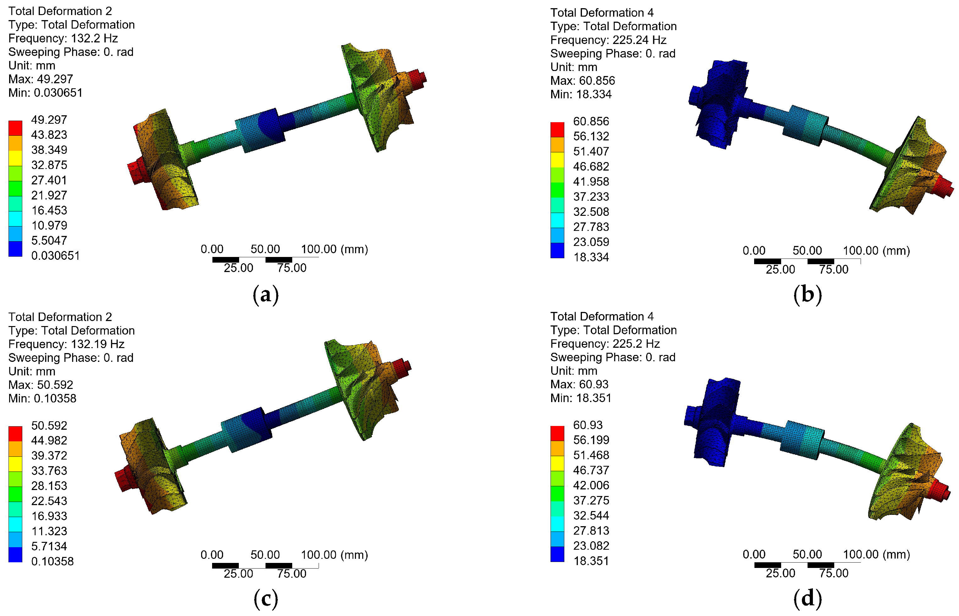
4.1. Model Validation

In order to verify the lumped parameter model in this paper, the modal analysis is now carried out using the finite element simulation which is performed in Workbench 2024 R1 to obtain the critical speed of the system and to compare the results with those obtained from the lumped mass method model.

The stiffness of rolling bearings is time-varying. Replace the stiffness of the bearings with K_eq to simplify the calculation.

In Equation (5), giving the solution to be $\mathit{q}=\mathit{u}{e}^{\lambda t}$, the characteristic equation can be expressed as

$$({\lambda }^2\mathbf{M}+\lambda (\omega \mathbf{G}+{\mathbf{C}}_1)+{\mathbf{K}}_1+{\mathbf{K}}_{\mathrm{eq}})\mathit{u}=\mathbf{0}$$

(62)

Transform it into a general generalized eigenvalue problem.

$$\left(\lambda \mathbf{P}+\mathbf{Q}\right)\left\{\begin{array}{c}\mathit{u}\\ \lambda \mathit{u}\end{array}\right\}=\mathbf{0}$$

(63)

where

$$\mathbf{P}=\left[\begin{array}{cc}\omega \mathbf{G}+{\mathbf{C}}_1& \mathbf{M}\\ \mathbf{M}& \mathbf{0}\end{array}\right] \mathbf{Q}=\left[\begin{array}{cc}{\mathbf{K}}_1+{\mathbf{K}}_{\mathrm{eq}}& \mathbf{0}\\ \mathbf{0}& -\mathbf{M}\end{array}\right]$$

(64)

The imaginary part of the eigenvalue λ is the natural frequency of the system. When the natural frequency and rotating speed are equal, the latter is the critical speed.

By setting k_eq = 10⁶ N/m, the vibration modes obtained by the lumped mass method and finite element model are shown in Figure 4 and Figure 5, respectively. In Figure 5, the mesh sizes at the turbine end and compressor end are 3.5 mm, 4 mm, and 4.5 mm for Type 1, Type 2, and Type 3, respectively, while the shaft segment mesh sizes are 1.5 mm, 2 mm, and 2.5 mm for Type 1, Type 2, and Type 3, correspondingly. Based on the comparative analysis of Figure 5 and

Table 1. The critical speeds calculated using the three types of meshes in the finite element model.

	First Resonance Mode	Second Resonance Mode
Mesh Type 1 (rpm)	9146	15,204
Mesh Type 2 (rpm)	9146	15,203
Mesh Type 3 (rpm)	9147	15,205

, the calculated deformations and critical speeds demonstrate excellent agreement across different mesh configurations, indicating that the numerical results have achieved satisfactory convergence. They both show that the first resonance mode is conical mode, and the second resonance mode is bending mode. The conical mode and bending mode, which have been reported by Ref. [21], commonly exist in turbocharger rotor systems. A comparison of critical speeds obtained from the lumped mass modeling and finite element modeling approaches is presented in

Table 2. Critical rotational speed of the first two orders of the two methods.

	Lumped Mass Model	Finite Element Model (Mesh Type 1)	Relative Error
First mode (rpm)	9956	9146	8.8%
Second mode (rpm)	14,020	15,204	7.8%

. It shows that the results of the two methods are relatively close.

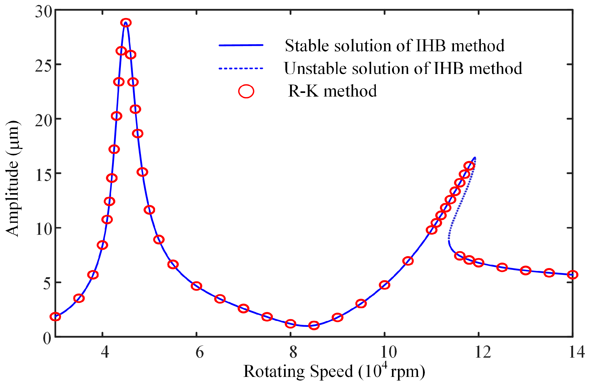
4.2. The Validation for the MIHB Method

From the vibration mode diagram, it can be seen that the amplitude of each lumped mass in the X direction is positively correlated with the amplitude in the Y direction under a steady state. Therefore, Y₁ can be used as an indicator to verify the results. In the subsequent discussion, the vertical axis is defined as

$$\mathrm{Amplitude}={\displaystyle \frac{1}{2}}[\max (B_{\tau }{\mathit{Y}}_1)-\min (B_{\tau }{\mathit{Y}}_1)]$$

(65)

In this paper, unless otherwise stated, the parameters of the turbocharger rotor are listed in

Table 3. System physical and material parameters.

Variable	Value	Variable	Value
m1 (kg)	0.46	Ja1 (kg·m2)	1.35 × 10−4
m2 (kg)	0.16	Ja2 (kg·m2)	5.83 × 10−6
m3 (kg)	0.17	Ja3 (kg·m2)	5.75 × 10−6
m4 (kg)	0.23	Ja4 (kg·m2)	6.71 × 10−5
l1 (mm)	16.0	Jp1 (kg·m2)	1.73 × 10−4
l2 (mm)	78.1	Jp2 (kg·m2)	1.17 × 10−5
l3 (mm)	22.6	Jp3 (kg·m2)	1.15 × 10−5
E1 (Pa)	2.1 × 1011	Jp4 (kg·m2)	9.35 × 10−5
E2 (Pa)	1.78 × 1011	e1 (m)	6.43 × 10−6
E3 (Pa)	2.08 × 1011	e4 (m)	1.28 × 10−6
I1 (m4)	3.87 × 10−9	I2 (m4)	1.29 × 10−8
I3 (m4)	1.99 × 10−9

, the parameters of the rolling bearing are listed in

Table 4. Initial parameters related to system constraints.

Physical Parameter	Variable	Value
Hertz contact stiffness (N/m1.5)	Cb	7.055 × 109
Number of rolling bearings	Nb	9
Initial radial clearances of rolling bearing (μm)	δ0	1.5
Equivalent linear stiffness (N/m) Equivalent linear damping coefficient (N·s/m)	kc cn	2.2 × 107 87
Diameter of inner ring (mm)	di	20.4
Diameter of outer ring (mm)	do	30.1
The first-order modal damping ratios	ξ1	0.021
The second-order modal damping ratios	ξ1	0.034

, and the MIHB preset parameters are listed in

Table 5. Preset parameter required for the MIHB method.

Preset Parameter	Variable	Value
Number of truncated harmonic terms	h	4
Error tolerance	Rt	1 × 10−9
Stepsize of iteration	z	10
Number of sampling points Maximum speed (rpm)	N ωmax	215 14 × 104

.

The validity and efficiency of the MIHB method can be demonstrated by comparisons of results between the R-K method and the MIHB method shown in Figure 6. Equation (5) was solved using MATLAB R2023a with an ode45 solver and relative tolerance set to 1 × 10⁻⁶. The amplitude represents the amplitude in the horizontal direction of the turbine end. The average computation time of a single rotating speed is about 60.4 s using the R-K method, while the average computation time is about 3.1 s using the MIHB method. Moreover, Figure 6 shows good consistency with traditional numerical methods, and it can track solution branches more comprehensively.

5. Discussion

The system exhibits bistable phenomena in Figure 6. Using the MIHB method, the frequency response characteristics of the turbine end can be obtained from the waterfall plot. As shown in Figure 7, the amplitude of the system comes from the synchronous vibration at the rotational frequency. There are resonance peaks at 4.5 × 10⁴ rpm and 11 × 10⁴ rpm, respectively. The bistable phenomena appear near the resonance frequency of the bending mode. Furthermore, as can be seen in Figure 7, the horizontal and vertical amplitudes at the turbine end are nearly identical. Therefore, in this model, the influence of the system’s gravity is negligible.

The influence of the distance between the equivalent linear constraint and the rolling bearing on the system vibration is shown in Figure 8. Note that the total length of the system has not changed. Only the position of the rolling bearing can be changed, and the change in l₂ is accompanied by the change in l₃. As l₂ increases, the resonance peak of the conical mode increases greatly, and the resonance peak of the bending mode decreases. More importantly, the resonance frequency of the conical mode increases slightly, and the resonance frequency of the bending mode increases greatly. Meanwhile, the speed range where bistable states occur is larger, which indicates the system is prone to amplitude jumps. Moreover, turbocharger usually operates under non-resonant rotating speed. Decreasing l₂ could decrease the vibration amplitude of the turbocharger rotor at low non-resonant rotating speed and strengthen the impact resistance of the system.

The influence of the number of balls in rolling bearings on the amplitude of the turbine end is shown in Figure 9. As N_b increases, the resonance peak of the conical mode increases, and the resonance peak of the bending mode decreases. The resonance frequency of the bending mode increases slightly, and the resonance frequency of the conical mode barely changes. Meanwhile, the speed range where bistable states occur narrows. Increasing N_b will increase the vibration amplitude of the turbocharger rotor at a non-resonant rotating speed and strengthen the impact resistance of the system.

The influence of bearing clearance on turbine end amplitude is shown in Figure 10. As the bearing clearance increases, the resonance peak of the conical mode increases significantly, and the resonance peak of the bending mode barely changes. The resonance frequency of the bending mode barely changes, and the resonance frequency of the conical mode decreases slightly. Meanwhile, the speed range where bistable states occur is much larger, which means the system is prone to amplitude jumps. Decreasing δ₀ will decrease the vibration amplitude of the turbocharger rotor at a non-resonant rotating speed and strengthen the impact resistance of the system.

Similar to the impact caused by changes in the number of balls, it can be seen in Figure 11 that as C_b increases, the resonance peak of the conical mode increases, and the resonance peak of the bending mode decreases. The resonance frequency of the bending mode increases slightly, and the resonance frequency of the conical mode barely changes. Meanwhile, the speed range where bistable states occur narrows. Increasing C_b will increase the vibration amplitude of the turbocharger rotor under non-resonant rotating speed and strengthen the impact resistance of the system.

The changes in the above parameters can barely cause the change of resonance peak of the conical mode, proving that the nonlinearity of the rolling bearing has a low correlation with the conical mode. As shown in Figure 12, increasing the equivalent linear stiffness of another bearing has almost no effect on the resonance peak of the bending mode, while it can effectively increase the resonance frequency of the conical mode and reduce its peak value.

As discussed earlier, the second-order resonance peak originates from the nonlinearity of rolling bearings. Its peak value may be significantly affected by the damping ratio of the second-order mode since ξ₂ can be adjusted by changing the physical parameters of the rolling bearing, such as temperature. The influence of second-order modal damping ratios on system vibration is shown in Figure 13. As ξ₂ increases, the change of ξ₂ almost only affects two resonance peaks. When ξ₂ increases, resonance peaks of the two modes will decrease simultaneously, especially of the conical mode.

Based on the data analysis results from Figure 8, Figure 9, Figure 10, Figure 11, Figure 12 and Figure 13,

Table 6. Sensitivity of resonant frequency and amplitude to parameter modifications.

Parameter	The Variation of the Parameter	The Variation Rate of the First-Order Resonant Frequency	The Variation Rate of the Second-Order Resonant Frequency	The Variation Rate of the First-Order Resonance Peak	The Variation Rate of the Second-Order Resonance Peak
l2 (mm)	74~86	−1.9~2.2%	−11.6~34.6%	−24.4~33.6%	27.1~−36.9%
Nb	8~12	−0.3~0.1%	−2.6~6.0%	−4.2~8.5%	2.8~−12.0%
δ0 (μm)	1~5	0.0~−1.3%	0.0~−1.8%	0.0~−50.87%	0.0~3.4%
Cb (N/m1.5)	6.055~10.055	−0.4~0.2%	−3.1~7.5%	−5.7~10.0%	6.5~−12.2%
kc (N/m)	1.5 × 107~2.5 × 107	−12.6~10.9%	−0.1~0.0%	15.9~−14.5%	−3.9~4.3%
ξ2	0.030~0.038	0.0~−0.1%	1.8~−1.2%	23.0~−16.0%	13.9~−9.6%

systematically presents the numerical sensitivity characteristics of various parameters. This sensitivity analysis, conducted by calculating the variation rates of vibration amplitude and resonance frequency relative to their initial values under parameter modifications, reveals the following key patterns: first, the bearing spacing parameter exerts significant influence on the system’s dynamic characteristics, particularly demonstrating remarkable control effects on both the second-order resonance frequency and the amplitudes of the first two resonance peaks. Second, variations in bearing clearance primarily affect the system’s first-order resonance peak, exhibiting exceptionally strong sensitivity.

6. Conclusions

This paper integrates a set of modeling and solving methods for the nonlinear dynamic characteristic of a turbocharger system supported by rolling bearings. Using the modified incremental harmonic balance (MIHB) method embedded in arc length continuation, systematic research is conducted on the nonlinear behavior of the turbocharger rotor system coupled with rolling bearings. Factors that may affect the amplitude of the system are analyzed systematically. Some meaningful conclusions are as follows:

(1)

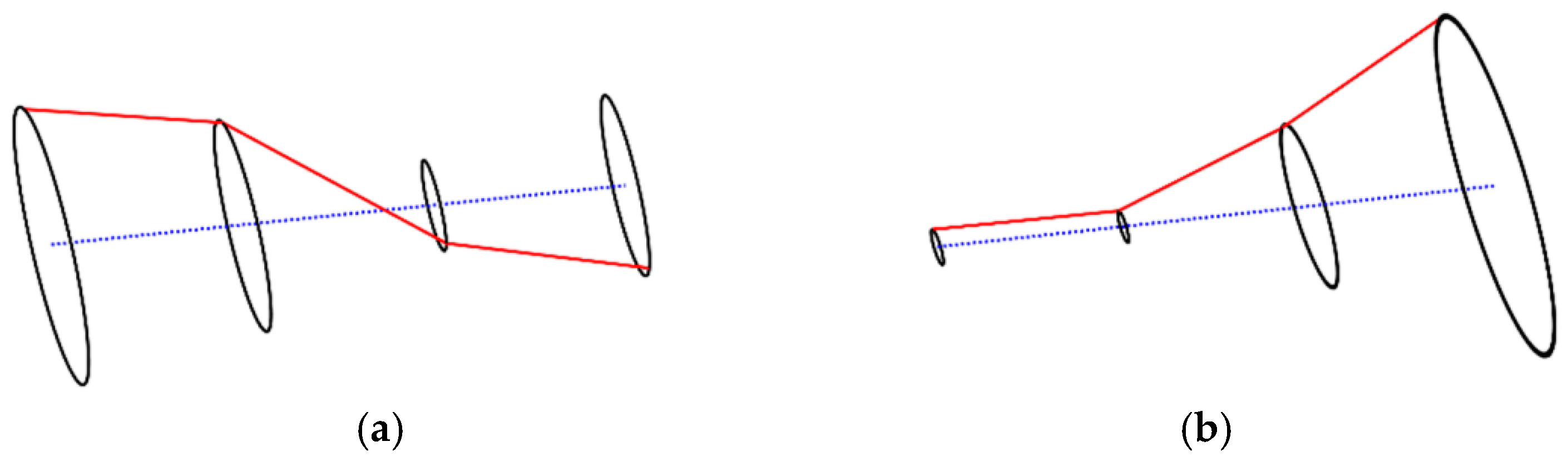
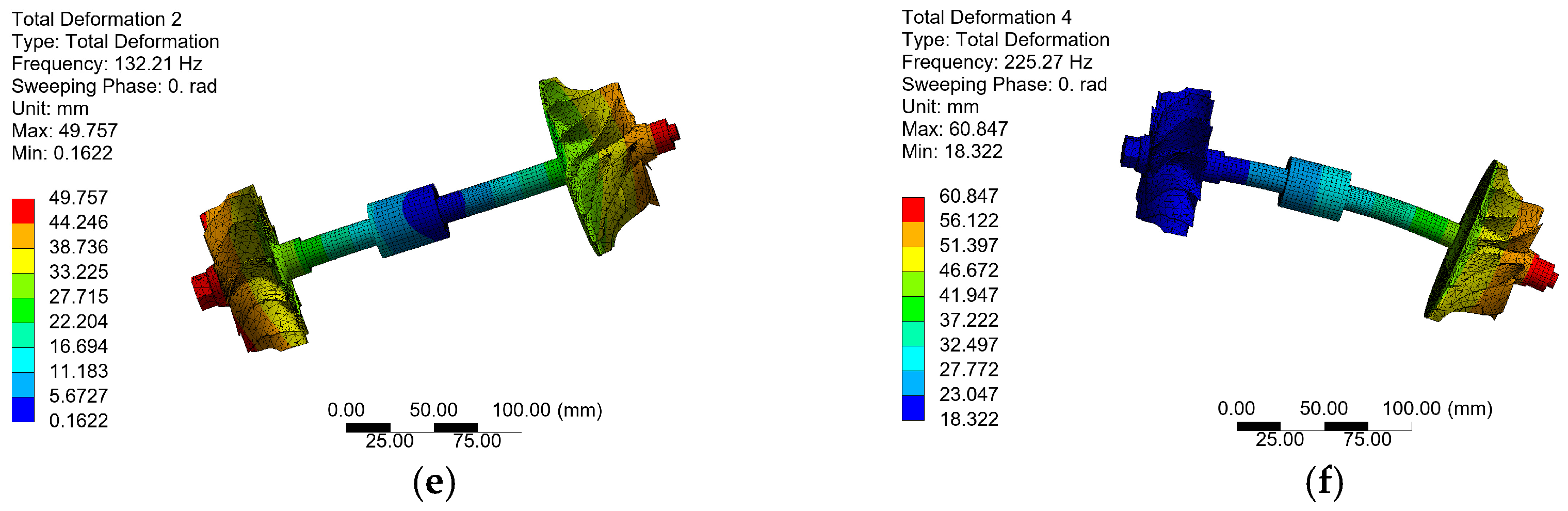
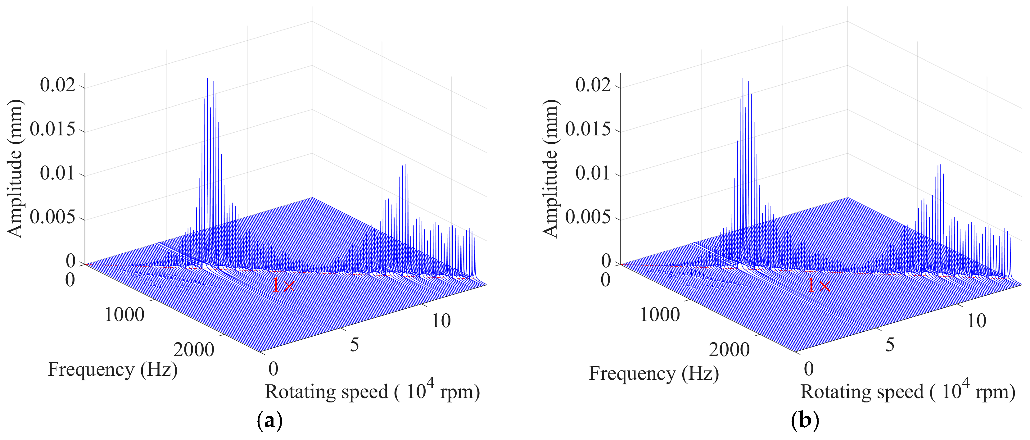
The resonance modes of the system at low speed (around 4.5 × 10⁴ rpm) and high speed (around 11 × 10⁴ rpm) are conical mode and bending mode, respectively, with a bistable phenomenon appearing at the resonance peak of the bending mode.

(2)

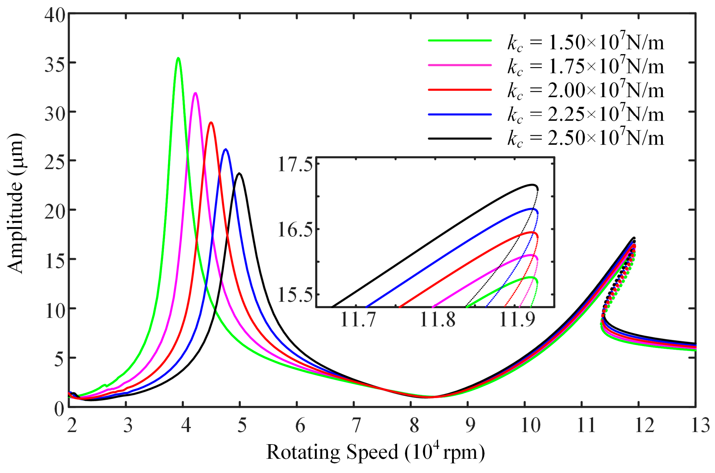
The conical mode resonance peak demonstrates notable sensitivity to both bearing clearance and the spacing between the two bearings. The amplitude of the system in the non-resonant speed range is positively correlated with the resonance peak of the conical mode. Therefore, when designing a turbocharger, the resonance peak of the conical mode should be suppressed. To achieve this, it is necessary to increase the equivalent stiffness of another bearing and reduce the distance between the two bearings.

(3)

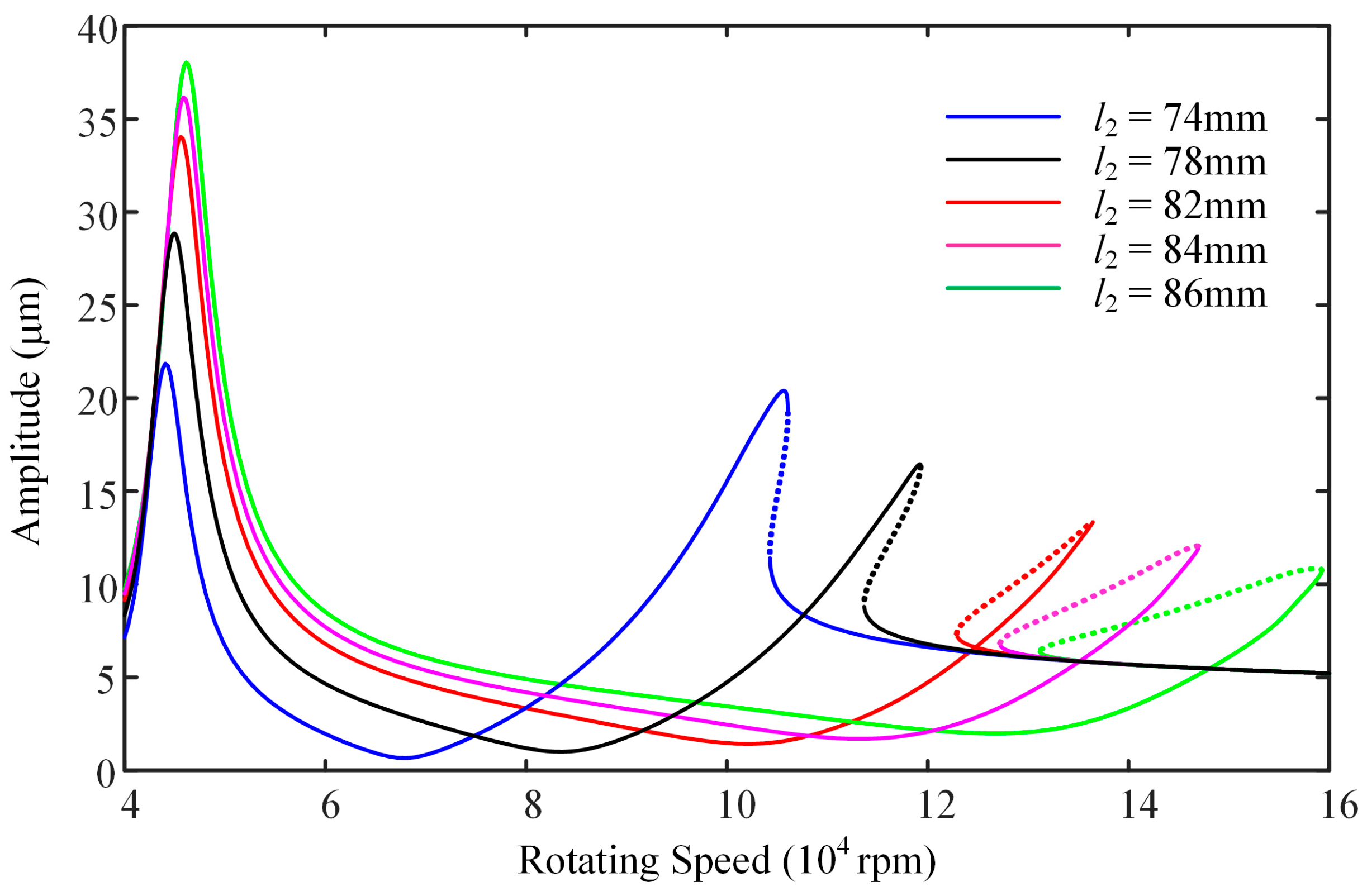
The bending mode’s resonance frequency and amplitude are highly sensitive to the spacing between the two bearings. Due to the fact that the resonance peak value of the bending mode is smaller than that of the conical mode, it is more important to reduce its bistable range compared to suppressing amplitude.

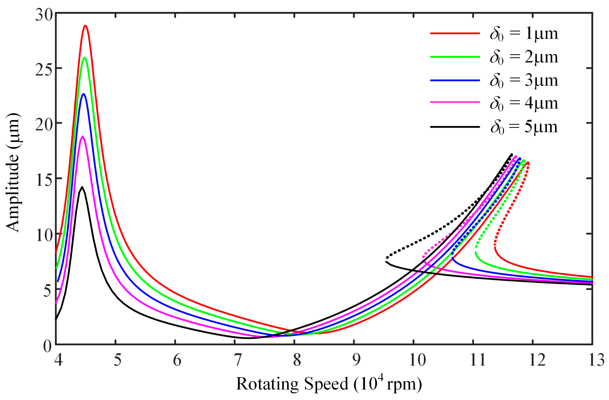
(4)

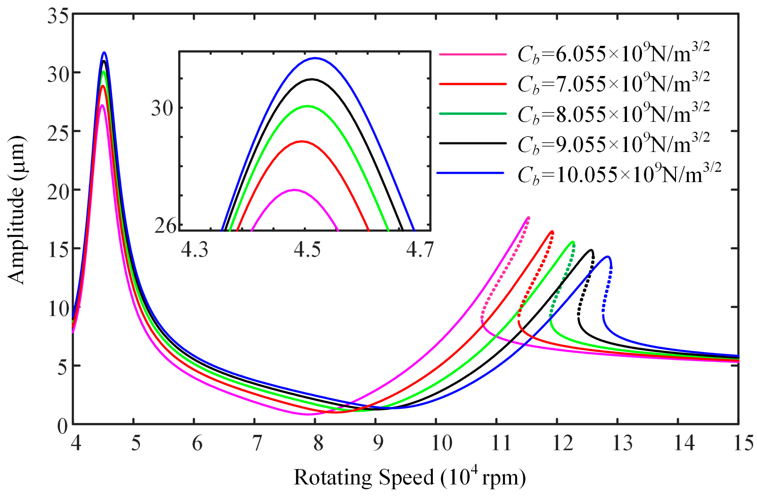
In general, the decrease of one vibration peak is often in the wake of the increase of another one unless increasing the modal damping ratio. Choosing bearings with a large number of ball bearings, high Hertz contact stiffness, and small bearing clearance can effectively prevent amplitude jumps and enhance the system’s impact resistance at high speeds. However, under non-resonant rotating speed, the amplitude will increase. Therefore, the equivalent stiffness of another bearing needs to be adjusted simultaneously. The distance between two bearings should be as small as possible while meeting other parameter requirements.

The parameter variations studied in this work can be further extended to uncertainty quantification, which is critical for the reliability-based design of turbochargers under real operating conditions. This study provides foundational support for automotive turbocharger design guidelines. The research enables precise adjustment of vehicular turbocharger constraints to prevent operational instability under impact loading conditions (e.g., when traversing rough terrain).

References

1. Nyongesa, A.; Park, M.; Lee, C.; Choi, J.H.; Hur, J.J.; Lee, W.J. Experimental evaluation of the significance of scheduled turbocharger reconditioning on marine diesel engine efficiency and exhaust gas emissions. Ain Shams Eng. J. 2024, 15, 102845. [Google Scholar] [CrossRef]
2. Wang, L.; Wang, A.; Yin, Y.; Heng, X.; Jin, M. Effects of unbalance orientation on the dynamic characteristics of a double overhung rotor system for high-speed turbochargers. Nonlinear Dyn. 2022, 107, 665–681. [Google Scholar] [CrossRef]
3. Cao, H.; Niu, L.; Xi, S.; Chen, X. Mechanical model development of rolling bearing-rotor systems: A review. Mech. Syst. Signal Proc. 2018, 102, 37–58. [Google Scholar] [CrossRef]
4. Singh, A.; Gupta, T.C. Effect of rotating unbalance and engine excitations on the nonlinear dynamic response of turbocharger flexible rotor system supported on floating ring bearings. Arch. Appl. Mech. 2020, 90, 1117–1134. [Google Scholar] [CrossRef]
5. Smolík, L.; Dyk, S. Towards efficient and vibration-reducing full-floating ring bearings in turbochargers. Int. J. Mech. Sci. 2020, 175, 105516. [Google Scholar] [CrossRef]
6. Peixoto, T.F.; Nordmann, R.; Cavalca, K.L. Dynamic analysis of turbochargers with thermo-hydrodynamic lubrication bearings. J. Sound Vib. 2021, 505, 116140. [Google Scholar] [CrossRef]
7. Ishida, Y.; Yamamoto, T. Linear and Nonlinear Rotordynamics: A Modern Treatment with Applications; John Wiley & Sons: New York, NY, USA, 2012. [Google Scholar]
8. Sawalhi, N.; Randall, R.B.; Endo, H. The enhancement of fault detection and diagnosis in rolling element bearings using minimum entropy deconvolution combined with spectral kurtosis. Mech. Syst. Signal Proc. 2007, 21, 2616–2633. [Google Scholar] [CrossRef]
9. Tian, J.; Wang, P.; Xu, H.; Ma, H.; Zhao, X. Nonlinear vibration characteristics of rolling bearing considering flexible cage fracture. Int. J. Non-Linear Mech. 2023, 156, 104478. [Google Scholar] [CrossRef]
10. Sunnersjö, C. Varying compliance vibrations of rolling bearings. J. Sound Vib. 1978, 58, 363–373. [Google Scholar] [CrossRef]
11. Fukata, S.; Gad, E.; Kondou, T.; Ayabe, T.; Tamura, H. On the radial vibration of ball bearings: Computer simulation. Bull. JSME 1985, 28, 899–904. [Google Scholar] [CrossRef]
12. Mevel, B.; Guyader, J. Routes to chaos in ball bearings. J. Sound Vib. 1993, 162, 471–487. [Google Scholar] [CrossRef]
13. Mevel, B.; Guyader, J. Experiments on routes to chaos in ball bearings. J. Sound Vib. 2008, 318, 549–564. [Google Scholar] [CrossRef]
14. Zhao, Y.; Hou, Y.; Wang, X.; Wei, J.; Shi, H.; Sha, C. A multiaxial fatigue method for rolling contact fatigue life prediction of axle box bearing under wheel-rail excitation conditions. Eng. Fail. Anal. 2024, 159, 108086. [Google Scholar] [CrossRef]
15. Andres, L.; Rivadeneria, J.; Chinta, M.; Gjika, K.; LaRue, G. Nonlinear rotordynamics of automotive turbochargers: Predictions and comparisons to test data. J. Eng. Gas Turbines Power 2007, 129, 488–493. [Google Scholar] [CrossRef]
16. Andres, L.; Rivadeneria, J.; Gjika, K.; Groves, C.; LaRue, G. A virtual tool for prediction of turbocharger nonlinear dynamic response: Validation against test data. J. Eng. Gas Turbines Power 2007, 129, 1035–1046. [Google Scholar] [CrossRef]
17. Andres, L.; Rivadeneria, J.; Gjika, K.; Groves, C.; LaRue, G. Rotordynamics of small turbochargers supported on floating ring bearings—Highlights in bearing analysis and experimental validation. J. Tribol. 2007, 129, 391–397. [Google Scholar] [CrossRef]
18. Bonello, P. Transient modal analysis of the non-linear dynamics of a turbocharger on floating ring bearings. J. Tribol. 2009, 223, 79–93. [Google Scholar] [CrossRef]
19. Tian, L.; Wang, W.J.; Peng, Z.J. Dynamic behaviours of a full floating ring bearing supported turbocharger rotor with engine excitation. J. Sound Vib. 2011, 330, 4851–4874. [Google Scholar] [CrossRef]
20. Tian, L.; Wang, W.J.; Peng, Z.J. Nonlinear effects of unbalance in the rotor-floating ring bearing system of turbochargers. Mech. Syst. Signal Process. 2013, 34, 298–320. [Google Scholar] [CrossRef]
21. Tian, L.; Wang, W.; Peng, Z. Effects of bearing outer clearance on the dynamic behaviours of the full floating ring bearing supported turbocharger rotor. Mech. Syst. Signal Process. 2012, 31, 155–175. [Google Scholar] [CrossRef]
22. Ouyang, X.; Guo, H.; Wu, X.; Men, R.; Li, M.; Cao, S. Investigation of weight effects on the critical speed of inclined turbocharger rotor system. J. Nonlinear Math. Phys. 2022, 29, 403–422. [Google Scholar] [CrossRef]
23. Kong, X.; Guo, H.; Cheng, Z.; Men, R. Dynamic characteristics of electrically assisted turbocharger rotor system under strong impacts. J. Vib. Eng. Technol. 2024, 12, 7955–7967. [Google Scholar] [CrossRef]
24. Mutra, R.R.; Srinivas, J.; Shaik, J.H.; Obaiah, M.C.; Balamurali, G.; Kumar, P. Turbocharger rotor vibration reduction methodology with an active control scheme. Noise Vib. Worldw. 2021, 52, 347–355. [Google Scholar] [CrossRef]
25. Liu, Y.; Liu, H. A coupled model of angular-contact ball bearing-elastic rotor system and its dynamic characteristics under asymmetric support. J. Vib. Eng. Technol. 2021, 9, 1175–1192. [Google Scholar] [CrossRef]
26. Ghaisas, N.; Wassgren, C.; Sadeghi, F. Cage instabilities in cylindrical roller bearings. J. Tribol. 2004, 126, 681–689. [Google Scholar] [CrossRef]
27. Zhao, H.; Fu, C.; Zhang, Y.Q.; Zhu, W.D.; Lu, K.; Francis, E.M. Dimensional decomposition-aided metamodels for uncertainty quantification and optimization in engineering: A review. Comput. Methods Appl. Mech. Eng. 2024, 428, 117098. [Google Scholar] [CrossRef]
28. Omid, M.; Saleh, M. Adaptive sliding mode control for finite-time stability of quad-rotor UAVs with parametric uncertainties. ISA Trans. 2018, 72, 1–14. [Google Scholar]
29. Fu, C.; Zhang, K.F.; Cheng, H.; Zhu, W.D.; Zheng, Z.L.; Lu, K.; Yang, Y.F. A comprehensive study on natural characteristics and dynamic responses of a dual-rotor system with inter-shaft bearing under non-random uncertainty. J. Sound Vib. 2024, 570, 118091. [Google Scholar] [CrossRef]
30. Ashtekar, A.; Tian, L.; Lancaster, C. An analytical investigation of turbocharger rotor-bearing dynamics with rolling element bearings and squeeze film dampers. In Proceedings of the 11th International Conference on Turbochargers and Turbocharging, London, UK, 13–14 May 2014; pp. 361–373. [Google Scholar]
31. Chang, Z.; Hou, L.; Chen, Y. Nonlinear dynamics and thermal bidirectional coupling characteristics of a rotor-ball bearing system. Appl. Math. Model. 2023, 119, 513–533. [Google Scholar] [CrossRef]
32. Kim, K.; Ri, K.; Yun, C.; Jong, Y.; Han, P. Nonlinear forced vibration and stability analysis of nonlinear systems combining the IHB method and the AFT method. Comput. Struct. 2022, 264, 106771. [Google Scholar] [CrossRef]
33. Lu, W.; Ge, F.; Wu, X.; Hong, Y. Nonlinear dynamics of a submerged floating moored structure by incremental harmonic balance method with FFT. Mar. Struct. 2013, 31, 63–81. [Google Scholar] [CrossRef]
34. Wang, X.; Zhu, W. A modified incremental harmonic balance method based on the fast Fourier transform and Broyden’s method. Nonlinear Dyn. 2015, 81, 981–989. [Google Scholar] [CrossRef]
35. Zhang, W.; Huseyin, K. Complex formulation of the IHB technique and its comparison with other methods. Appl. Math. Model. 2002, 26, 53–75. [Google Scholar] [CrossRef]
36. Ri, K.; Ri, Y.; Yun, C.; Kim, K.; Han, P. Analysis of nonlinear vibration and stability of Jeffcott rotor supported on squeeze-film damper by IHB method. AIP Adv. 2022, 12, 025127. [Google Scholar] [CrossRef]
37. Ri, K.; Jang, J.; Yun, C.; Pak, C.; Kim, K. Analysis of subharmonic and quasi-periodic vibrations of a Jeffcott rotor supported on a squeeze-film damper by the IHB method. AIP Adv. 2022, 12, 055328. [Google Scholar] [CrossRef]
38. Ju, R.; Fan, W.; Zhu, W. An efficient Galerkin averaging-incremental harmonic balance method based on the fast Fourier transform and tensor contraction. J. Vib. Acoust. 2020, 142, 1–38. [Google Scholar] [CrossRef]
39. Chang, Z.; Hou, L.; Lin, R.; Jin, Y.; Chen, Y. A modified IHB method for nonlinear dynamic and thermal coupling analysis of rotor-bearing systems. Mech. Syst. Signal Proccess. 2023, 200, 110586. [Google Scholar] [CrossRef]
40. Chang, Z.Y.; Hou, L.; Masarati, P.; Lin, R.Z.; Li, Z.G.; Chen, Y.S. Modeling and nonlinear analysis of a coupled thermo-mechanical dual-rotor system. Nonlinear Dyn. 2024, 112, 17811–17842. [Google Scholar] [CrossRef]
41. Chen, Y.; Hou, L.; Lin, R.Z.; Song, J.Z.; Ng, T.Y.; Chen, Y.S. A harmonic balance method combined with dimension reduction and FFT for nonlinear dynamic simulation. Mech. Syst. Signal Proccess. 2024, 221, 111758. [Google Scholar] [CrossRef]
42. Chen, Y.; Hou, L.; Lin, R.Z.; Toh, W.; Ng, T.Y.; Chen, Y.S. A general and efficient harmonic balance method for nonlinear dynamic simulation. Int. J. Mech. Sci. 2024, 276, 109388. [Google Scholar] [CrossRef]
43. Yang, Y.; Liu, C.; Lai, S.K.; Chen, Z.; Chen, L. Frequency-dependent equivalent impedance analysis for optimizing vehicle inertial suspensions. Nonlinear Dyn. 2025, 113, 9373–9398. [Google Scholar] [CrossRef]
44. Zhou, Y.; Luo, Z.; Bian, Z.; Wang, F. Nonlinear vibration characteristics of the rotor bearing system with bolted flange joints. Proc. Inst. Mech. Eng. Part K 2019, 233, 910–930. [Google Scholar] [CrossRef]
45. Roy, H.; Chandraker, S.; Dutt, J.K.; Roy, T. Dynamics of multilayer, multidisc viscoelastic rotor-An operator based higher order classical model. J. Sound Vib. 2016, 369, 87–108. [Google Scholar] [CrossRef]
46. Kluger, J.; Crevier, L.; Udengaard, M. Speed-dependent eigenmodes for efficient simulation of transverse rotor vibration. Vibration 2022, 5, 732–754. [Google Scholar] [CrossRef]
47. Harris, T.; Kotzalas, M. Rolling Bearing Analysis: Essential Concepts of Bearing Technology; CRC Press: Boca Raton, FL, USA, 2006. [Google Scholar]
48. Zhang, H.; Zhai, J.; Han, Q.; Sun, W. Dynamics of a geared parallel-rotor system subjected to changing oil-bearing stiffness due to external loads. Finite Elem. Anal. Des. 2015, 106, 32–40. [Google Scholar] [CrossRef]
49. Chen, Y.; Hou, L.; Lin, R.; Wang, Y.; Saeed, N.A.; Chen, Y. Combination resonances of a dual-rotor-bearing-casing system. Nonlinear Dyn. 2024, 112, 4063–4083. [Google Scholar] [CrossRef]
50. Han, Y.; Ri, K.; Yun, C.; Kim, K.; Kim, K. Nonlinear vibration analysis and stability analysis of rotor systems supported on SFD by combining DQFEM, CMS and IHB methods. Appl. Math. Model. 2023, 121, 828–842. [Google Scholar] [CrossRef]
51. Zhu, G.; Lu, K.; Cao, Q.; Huang, P.; Zhang, K. Dynamic behavior analysis of tethered satellite system based on Floquet theory. Nonlinear Dyn. 2022, 109, 1379–1396. [Google Scholar] [CrossRef]
52. Berenguer, M.; Garbayo, A.; Mas, J.; Ramallo, A.V. Holographic Floquet states in low dimensions (II). J. High Energy Phys. 2022, 2022, 20. [Google Scholar] [CrossRef]
Figure 1. Simplified turbocharger rotor system model.
Machines 13 00360 g001
Figure 2. Schematic diagram of the rolling bearing.
Machines 13 00360 g002
Figure 3. Solution process of the MIHB method.
Machines 13 00360 g003
Figure 4. The first two resonance modes of the lumped mass model. (a) The first resonance mode; (b) the second resonance mode.
Machines 13 00360 g004
Figure 5. The first two resonance modes of the finite element model. (a) The first resonance mode, Mesh Type 1; (b) the second resonance mode, Mesh Type 1; (c) the first resonance mode, Mesh Type 2; (d) the second resonance mode, Mesh Type 2; (e) the first resonance mode, Mesh Type 3; (f) the second resonance mode, Mesh Type 3.
Machines 13 00360 g005aMachines 13 00360 g005b
Figure 6. Comparisons between the MIHB method and the R-K method.
Machines 13 00360 g006
Figure 7. Waterfall plot of frequency response at the turbine end. (a) Horizontal direction; (b) vertical direction.
Machines 13 00360 g007
Figure 8. The variation of the amplitude in the turbine end with the distance between bearings and equivalent linear constraints.
Machines 13 00360 g008
Figure 9. The variation of the amplitude in the turbine end with the number of balls.
Machines 13 00360 g009
Figure 10. The variation of the amplitude in the turbine end with bearing clearance.
Machines 13 00360 g010
Figure 11. The variation of the amplitude in turbine end with Hertz contact stiffness of rolling bearings.
Machines 13 00360 g011
Figure 12. The variation of the amplitude in the turbine end with equivalent linear stiffness of another bearing.
Machines 13 00360 g012
Figure 13. The variation of the amplitude in the turbine end with second-order modal damping ratios.
Machines 13 00360 g013