Abstract
Applying bionic airfoils is essential in enlightening the design of rotating machinery and flow control. Dynamic mode decomposition was used to reveal the low dimensional flow structure of Riblets, Seagull, and Teal bionic airfoils at low Reynolds numbers 1 × 10⁵ and is compared with NACA4412 airfoils. The attack angle of the two-dimensional airfoil is 19°, and the SST k-ω turbulence model and ANSYS fluent were used to obtain the transient flow field data. The sparse identification of nonlinear dynamics reveals the nonlinear correlation between modal coefficients and establishes manifold dynamics. The results show that the bionic airfoil and NACA4412 airfoil have the same type of nonlinear correlation, and the dimension and form of the minimum reduced-order model are consistent. The modal coefficients always appear in the manifold equation in pairs with a phase difference of 90°. The dimension of the manifold equation is two-dimensional, and the absolute value of the coefficient corresponds to the fundamental frequency of airfoil vortex shedding. The reconstructed flow field based on the manifold equation is highly consistent with the numerical simulation flow field, which reveals the accuracy of the manifold equation. The relevant conclusions of this study emphasize the unity of the nonlinear correlation of bionic airfoils.
1. Introduction
Civil or military equipment such as small wind turbines, micro air vehicles, and un-crewed aerial vehicles are operating at a low Reynolds number of 105 [1,2,3]. Airfoil stall and boundary layer separation may occur when the equipment is started at low wind speed and operated at high wind speed. The airfoil will generate less lift and more drag far from the separation point [4], and the unstable characteristics of the airfoil wake will cause structural vibration [5]. These highly nonlinear transient flows will significantly reduce the aerodynamic performance and even shorten the fatigue life of the equipment [6,7]. The nonlinear dynamics of airfoil stalls [8] have been a broad concern, and many studies have been used to delay airfoil stalls [9,10,11], predict the unstable behavior of separation [12], and operate under off-design conditions [13]. The ongoing learning and imitation of human beings from the biological world have promoted the rapid development of bionics, especially the development of bird wing kinematics. Bionic airfoils are applications of bionics to airfoils and inspired new ideas in airfoil design and flow control [14]. Therefore, it is essential to fully understand the nonlinear characteristics of the bionic airfoil stall to improve the airfoil performance.
Nature provides an endless treasure trove of inspiration for scientists and engineers in different fields [15,16,17]. After competition and evolution for survival, many animals have developed unique and superior flying or swimming skills, such as the silent flight of owls and the maneuverability of humpback whales. The flow and noise reduction mechanisms of biomimetic structures (sawtooth [18,19,20], wavy [21,22,23], and protuberance [24,25,26]) have been extensively studied. Pereira [27] conducted detailed measurements of the flow field and pointed out that the serrated trailing edge structure would significantly reduce the transport velocity of turbulent eddies. The spanwise correlation of wall pressure pulsations would also be reduced. Wang et al. [28] pointed out that the leading edge sawtooth bionic airfoil can be reduced by 14.3 dB compared to NACA0012. Li [29] et al. studied the aerodynamic characteristics of multi-protrusion airfoils and found that when the protrusion spacing is 0.25 times the chord length, the lift-to-drag ratio can be increased by 5% to 15%. The spaced and non-spaced double-protrusion airfoils show two-stage and one-side stall characteristics, respectively. The multi-protrusion airfoil still shows good lift characteristics at large angles of attack. Huang [30] et al. constructed a bionic airfoil with the leading-edge shape of the NACA0018 airfoil by imitating the shape of the dolphin head. When the airfoil attack angle was 16° and the deflection angle of the dolphin head was 24°, the lift coefficient can be increased by 21.1%, and the drag coefficient can be decreased by 29.8%.
The biomimetic shape of the airfoil has also received extensive attention besides the derived structures. Liu [31] measured the surface geometry of bird wings of a seagull, merganser duck, teal, and long-eared owl through a 3D laser scanning system and extracted geometric characteristics such as arc and thickness distribution, which provided information for the development and application of bionic airfoils. The seagull airfoil [32] has a higher lift-to-drag ratio and improves flow separation, which is more suitable for the blade design of small wind turbines than the NACA4412 airfoil. Li [33] et al. pointed out that the bionic airfoil composed of 40% of the cross-section of the long-eared owl slows down the range of vortex shedding by increasing the distance between the center of the vortex and the wall [34]. Zargar et al. [35] analyzed flow patterns and aerodynamic performance with different riblet airfoils in combination with particle image velocimetry. Although the flow mechanism of bionic airfoils has been reported in detail and many engineering applications have been implemented, the difference and unity of nonlinear dynamics have yet to be revealed.
Recently, modal analysis methods such as proper orthogonal decomposition (POD) [36] and dynamic mode decomposition (DMD) [37] have been used to reveal the low-dimensional structures of complex flows such as airfoils and to build reduced-order models. For example, significant success has been achieved in analyzing the dynamic stall phenomenon of airfoils [38,39,40]. The mode reflects the low dimensional characteristics of complex flow in space, and the mode coefficient represents the evolution law of the mode. Callaham et al. [41] exploited nonlinear correlations in modal coefficients to identify potential attractors and model interpretable dynamical systems. They show that the quasi-periodic shear cavity flow evolves on the torus produced by two independent Stuart-Landau oscillators, which is vital for revealing the physics of complex flows. Although many mechanism studies have been performed on bionic airfoils such as owls and seagulls, there is a lack of perspective to analyze the complex flow of bionic airfoils from the perspective of modal coefficients.
This study aims to construct an interpretable reduced-order model using the DMD modal coefficients of the airfoil and compare the differences between the NACA4412, Riblets, Seagull, and Teal airfoil. The minimum order manifold dynamics are further established based on the nonlinear correlation between the modal coefficients.
In the second part, the numerical simulation results of the NACA4412 airfoil are compared with the experiments to verify the accuracy of the numerical method, and the airfoil flow field data at an attack angle of 19° are further obtained. In Section 3, the DMD is briefly introduced, and the randomized dependence coefficient (RDC) between the main modes of the airfoil and the modal coefficients are shown. In Section 4, the sparse identification of nonlinear dynamics (SINDy) proposed by Burunton et al. [42] is briefly introduced, and a two-dimensional manifold dynamics equation is constructed based on non-linear correlation. The main conclusions of this study are given in Section 5.
2. Test Case
2.1. Geometric Construction
This study mainly refers to the study of Liu et al. [31] to construct a biomimetic airfoil. The profile distribution of the upper and lower surfaces of the bionic airfoil can be obtained from the mid-arc line Zu and the thickness distribution relationship Zt. The control equation for the corresponding profile is:
The relationship between the mid-arc line and the thickness distribution is mainly determined by the maximum camber Zc,max and the maximum thickness Zt,max of the airfoil:
where η = x/c is the normalized chordwise coordinate. The x and c are the coordinates and chord length of the airfoil, respectively. The Sn and An are the coefficients describing the bionic airfoil, as shown in Table 1. The chord length c of the airfoil in this study is one meter.

Table 1.
Coefficient distribution of bionic airfoil.
The fitting relationship between the maximum camber Zc,max and the maximum thickness Zt,max of the bionic airfoil is:
where χ is the airfoil aspect ratio. As shown in Table 2, a, b and d are all coefficients describing the maximum camber and thickness. The subscripts c and t denote the maximum camber and maximum thickness, respectively.
Table 2.
Coefficient distribution for maximum camber and thickness.
The 40% spanwise direction of the bionic airfoil was selected, and the shape of the bionic airfoil obtained by coefficients such as mid-arc and thickness is shown in Figure 1. The shapes of the three airfoils are pretty different, with the NACA4412 airfoil looking fat, the seagull airfoil being curved, and the teal airfoil being thin.

Figure 1.
The geometry of the bionic airfoil (NACA4412, Riblets, Teal, and Seagull).
In addition to comparing the unity of airfoil ROMs with different geometric structures, this study also emphasizes the unity of the nonlinear correlation of riblet micromachined surfaces on airfoils. Figure 1 shows the riblets of the NACA4412 airfoil. Riblet micro serrations with a height of 0.1 mm and a width of 0.1 mm are uniformly distributed on the upper airfoil surface within the range of 0.7 c.
2.2. Numerical Method and Experimental Verification
In order to minimize the influence of the leading edge by the fluid disturbance at the inlet boundary and satisfy the flight state of real birds, the widely used C-shaped computational domain structure [43,44,45] was adopted. The airfoil chord length c in this study is 1 m. As shown in Figure 2, the first half of the computational domain is a semicircle (10 times the chord distance), and the downstream part is a rectangle (20 times the chord distance). The Reynolds number Re, Strouhal number St, and lift coefficient CL of an airfoil is defined as follows:
where ρ, U and c are the density of the fluid, the incoming velocity, and the airfoil chord length, respectively. The μ, f and FL are the dynamic viscosity of the fluid, the vortex shedding frequency, and the surface lift of the airfoil, respectively.
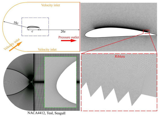
Figure 2.
Computational Domains and Grids.
The airfoil in this study operates at a low Reynolds number, the corresponding density is constant, and the governing equation is an incompressible Reynolds averaged Navier-Stokes (RANS) equation:
where ui and uj are the velocity components. μ, , and are the dynamic viscosity, average pressure, and Reynolds stresses, respectively.
The airfoil grid was generated by the commercial software ANSYS Icem, which adopts the division method of a structural or unstructured grid. The large number of tiny serrations on riblets are tricky to construct geometrically and challenging to grid. This study used a fine unstructured grid near the tiny serrations, and the boundary layer was drawn on the rest of the airfoil surface. The NACA4412, Teal, and Seagull airfoil were divided into structural grids. The low-dimensional structure of the airfoil vortex shedding was considered, and the mesh around the airfoil was sufficiently refined. The height of the first grid on the airfoil wall is 0.05 mm, and the grid growth rate is 1.03.
The commercial software ANSYS Fluent 2022 R1 and CFD-POST were used to solve unsteady flow and statistical flow field data. Python was used for further dynamic mode decomposition to obtain main modes and analyze nonlinear correlation. The fluid medium is air (density 1.225 kg/m3, dynamic viscosity 1.7894 × 10⁻⁵ Pa·s). Figure 2 shows the unified boundary conditions and different grid details. The inlet and outlet of the airfoil basin are the velocity inlet and zero pressure outlet. The direction of inlet velocity matches the airfoil angle of attack, and the turbulence intensity and viscosity are 5% and 10%, respectively. The airfoil and riblets are non-slip walls, and the turbulence model is the SST k-ω turbulence model [46]. The pressure-velocity coupling scheme is SIMPLE, and under-relaxation factors are Pressure = 0.3, Density = 1, Body Forces = 1, Momentum = 0.7, Turbulent Kinetic Energy = 0.8, Specific Dissipation Rate = 0.8, and Turbulent Viscosity = 1. The Gradient is least squares cell-based, and the Pressure interpolation scheme is second order. The second-order upwind and central difference schemes are used for the advective and diffusive fluxes in the governing equations discretized, respectively. The Transient Formulation is second-order implicit. The residual of continuity, x-velocity, y-velocity, k, and ω is 10−6.
The stall characteristics at a large attack angle of 19° under a low Reynolds number of 1 × 10⁵ were studied. The time step is 0.001 s. After the lift coefficient fluctuates periodically, the calculated data of each time step is saved and used as the snapshot data of the DMD. Four different grid numbers are used for grid-independent verification to ensure the validity of the grid. Figure 3a shows that for NACA4412, Teal, and Seagull when the grid number is more than 0.2 million, the fluctuation range of St is within 0.5%. Figure 3b shows that when the grid number of ridged airfoils is more than 0.7 million, the fluctuation of St can be ignored. Considering the details of the flow field and mode, the grids of NACA4412, Teal, Seagull, and Riblets airfoil are 0.39, 0.35, 0.39, and 1.54 million, respectively.
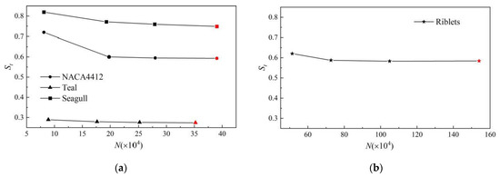
Figure 3.
Grid independence verification. (a) NACA4412, Teal and Seagull, (b) Riblets.
The effect of different time steps Δt on the St of the Teal airfoil is further studied because the vortex shedding period of the Teal airfoil is the smallest. Figure 4 shows that the influence of four different time steps on the St of the canard airfoil can be ignored. The main reason is that there are still 100 calculation steps in a vortex shedding cycle corresponding to the maximum time step. Due to the low consumption of two-dimensional computing resources, the time step in this study is 0.001 s.
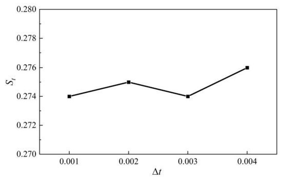
Figure 4.
Independence verification of time step Δt.
Figure 5 compares the lift coefficients of the NACA4412, Riblets, Seagull, and Teal. The lift coefficient of the Seagull bionic airfoil has enormous improvement. Table 3 shows the vortex shedding frequencies for the four airfoils, where the angular frequency ω = 2f. Many micro serrations on the Riblets airfoil surface did not significantly change the vortex shedding frequency of NACA4412, and the lift coefficient decreased slightly. The Seagull airfoils vortex shedding frequency and lift coefficient are significantly higher than the other three airfoils.

Figure 5.
The lift coefficients CL of NACA4412, Riblets, Seagull, and Teal airfoil.
Table 3.
Vortex shedding angular frequency and St number.
The static stall characteristics of the NACA4412 airfoil at a Reynolds number of 1.52 × 10⁶ are simulated to verify the effectiveness of the numerical method. Figure 6 compares the numerical simulation and experimental results of Coles [47] and Pinkerton [48]. The numerical simulation results are in good agreement with the experimental results (lift coefficient CL), which proves that the numerical simulation of the two-dimensional airfoil in this study is compelling and reliable.
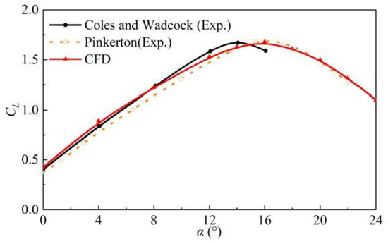
Figure 6.
Comparison of Numerical Simulation and Experiment.
According to Noack et al. [49] and Loiseau et al. [50] adopting a layered approach, decomposing the velocity u into the average velocity () and the fluctuation velocity () can better reflect the nonlinear correlation between the velocity [30]. In the follow-up research, the dynamic mode decomposition of the fluctuation velocity field of the airfoil is mainly carried out.
3. Nonlinear Dependence of Modal Coefficients
3.1. Dynamic Mode Decomposition
Dynamic modal decomposition can reduce the dimension of the flow field and show the evolution of these modes with time (modal coefficients). Measuring the mode evolution with time is imperative in building the reduced order model. Although the flow field of an airfoil is highly nonlinear, DMD, similar to the Koopman operator [51], is often used for flow field reduction and mechanism analysis. DMD is wholly based on data measurement and does not need any knowledge of control equations. The combination of DMD and modal analysis, such as POD, has also been extensively studied. DMD has good predictive capabilities and is also used in applications such as bearing fault diagnosis [52]. This study gives a brief introduction to DMD modes and modal coefficients.
The snapshot data of the airfoil can be divided into two matrices: X = [x(t1), x(t2), …, x(tm−1)] and X′ = [x(t2), x(t3), …, x(tm)]. The DMD seeks the best fitting linear operator A for these two matrices: X′ = AX. It is not easy to directly calculate operator A, whose dimension is the square of the airfoil flow field dimension. Therefore, the singular value decomposition (SVD) of matrix X is required in advance.
(1) Calculate the SVD of the data matrix X:
where the selection of low-rank r depends on the accuracy of low-dimensional modal reconstruction. The low-rank r in this study was chosen as twenty because the first twenty modes can accurately represent the entire physical field. The matrix and are left singular matrices and the right singular value matrix. The matrices and are unitary matrices, and each column is orthogonal. Each element on the main diagonal of matrix is a singular value of matrix X.
(2) The reduction linear operator is obtained by the matrices , , X′, and singular value matrix :
(3) The spectral decomposition of the matrix is calculated:
where W and the diagonal entries μj of the diagonal matrix are the eigenvector and eigenvalues of the approximate matrix . The eigenvalues λj of the DMD modes can be obtained from μj and sampling time Δt:
The real and imaginary parts of λj correspond to the mode growth or decay rate and frequency, respectively.
(4) The mode Φ according to the matrix W and X′ is obtained:
The reconstructed flow field x(t) is:
where βj(t) is the DMD modal coefficient, the accuracy of the reduced-order model constructed in this study mainly depends on the accuracy of the modal coefficient reconstruction. bj is the amplitude of the mode:
Five thousand snapshots (Total time t = 5 s) were collected for the airfoil DMD. The sampling interval is two times the time step (sampling frequency = 500 Hz). Since the vortex shedding structure of the airfoil is focused on, and to save memory and reduce mode decomposition time, the velocity around the airfoil (−c ≤ x ≤ 5c, −2c ≤ y ≤ 2c) was sampled. In particular, since the Riblets airfoil has many tiny serrations, it is necessary to extract more effective numerical velocity fields to ensure the details of the flow field near the serrations.
The spatial dimension of the DMD decomposition matrix corresponds to the number of grids in the sampling area. The modes are ordered according to the increasing frequency of the modes, mainly to obtain a unified nonlinear correlation. From the following research results, if the energy-decreasing order of modes is adopted, the frequency distribution of the Teal airfoil is chaotic (2ω, 4ω, ω, 6ω, 8ω, 3ω, 10ω, 5ω, 12ω, 7ω), which is not conducive to unifying nonlinear correlation.
The spatial distribution of airfoil modes shown in Figure 7 is consistent with the research of Naderi et al. [38], Moreover, the other modes are pure harmonics of the primary mode (corresponding to the mode of vortex shedding fundamental frequency). The modes of airfoils are antisymmetric vortex-shedding structures. The NACA4412, Riblets, and Seagull airfoil modes are similar to a certain extent. Under a large number of tiny serrations, the vortex-shedding structure in the middle of the upper surface of the Riblets airfoil disappears, and the high-frequency trailing edge vortex-shedding structure is different from the NACA4412 airfoil. For NACA4412, Riblets, and Teal airfoil modes, laminar separation bubbles (LSB) at the leading edge can be observed, and the Teal airfoil is the most obvious. The modes of the trailing edge of the four airfoils have obvious boundaries, indicating that the trailing edge vortex shedding is related to the shear layer near the trailing edge [53].
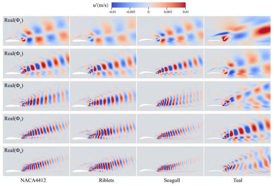
Figure 7.
Mode comparison of the NACA4412, Riblets, Seagull, and Teal airfoil.
The mode of Seagull airfoil mainly reflects the trailing edge vortex shedding, and no leading-edge LSB leads to a significant increase in lift coefficient CL. The modal of the Teal airfoil is different from the other three airfoils. The vortex shedding distribution range of the high-frequency trailing edge is higher than that of other airfoils. The frequency of the four airfoil modes is highly consistent with the frequency of the lift coefficient CL in Figure 5, indicating that the stall of the four airfoils is related to the shedding process of the Karman vortex [14].
The modal coefficients of these four airfoils are not explicitly shown in this study because the flow field of the airfoil is periodic, and the modal evolution over time is purely oscillatory. The difference between modal coefficients is mainly reflected in amplitude and phase. Therefore, the evolution of the airfoil flow field is periodic, with pure oscillation and dual frequency.
The flow field with fewer dimensions and simple nonlinear correlation can be realized by keeping the appropriate number of modes. When the number of reserved modes is 20, we can accurately express the velocity field of the airfoil using the modes. Figure 8 shows the accuracy of the flow field reconstruction of the first 20-order airfoils. The fluctuating velocity distribution is consistent with the CFD. The angular frequencies corresponding to the 20 modes of the airfoil are (ω, 2ω, …, 10ω), and the frequencies are multiples.
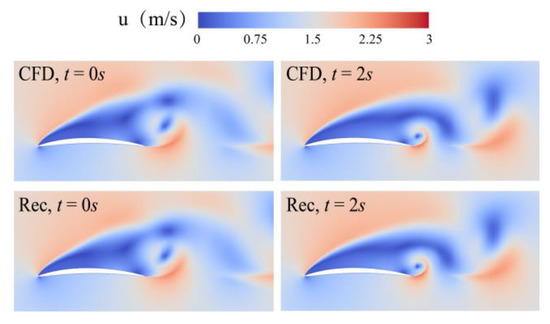
Figure 8.
Flow reconstruction of a Teal airfoil.
3.2. Nonlinear Correlation
The randomized dependence coefficient (RDC) proposed by Lopez-Paz et al. [54] was used to measure the nonlinear correlation between the modal coefficients βj(t). The RDC algorithm is simple and computationally inexpensive, and extending to nonlinear correlations between modal coefficients is easy. Figure 9 shows the Lissajous orbits and RDC for the first 20 modal coefficients of the NACA4412 airfoils. Since a modal coefficient is a complex number, and a pair of modal coefficients of the DMD are complex conjugates:
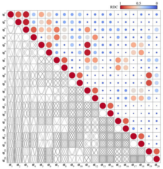
Figure 9.
The Lissajous orbits (lower left corner) and RDC distribution (the upper right corner) for the NACA4412 airfoil.
Four different airfoils have similar Lissajous orbits and RDC distributions. The main reason is the multiple relationships between frequency and the periodicity of flow. The modal coefficients are linearly uncorrelated, which does not mean there is no nonlinear correlation. Figure 9 shows that Lissajous orbits between each pair of modal coefficients are circular, indicating that the phase difference between a pair of modal coefficients is 90°. The nonlinear correlation between modal coefficients is very complex, but Lissajous orbits are ordered, and the distribution of RDC is sparse. This combination of order and sparsity is conducive to building specific functional relationships of nonlinear correlation.
4. Construction of the Minimum Reduced-Order Model
4.1. The Sparse Identification of Nonlinear Dynamics
Although RDC and Lissajous orbits show the nonlinear correlation between modal coefficients, the key to building a ROM is to use specific functional expressions to reflect the nonlinear correlation. The sparse identification of nonlinear dynamics (SINDy) proposed by Brunton et al. [42] plays a vital role in discovering control equations [55] in various fields, implementation of active control, construction of manifold equations, and other applications. Here is a brief introduction to SINDy.
A large number of nonlinear dynamic systems can be written as:
f(x) is approximated:
where matrix Θ(x) and ξ are the nonlinear function library and sparse matrix, the components of SINDy are similar to the DMD modes and modal coefficients. The sparse matrix ξ represents the sparsity of the function library rather than the evolution law of the nonlinear function library Θ(x). The more sparse the matrix means fewer dominant items in the function library (the more straightforward the nonlinear dynamic system). The key to SINDy is to build a function library Θ(x) and solve a sparse matrix ξ. The construction of a function library can give full play to the subjective initiative. The function library can be a polynomial, trigonometric, or exponential function:
The X consists of the series data X = [α(t1), α(t2), …, α(tm)]T.
Solving the sparse matrix Ξ is the core given the library Θ(x). The forward regression orthogonal least squares (FROLS) algorithm proposed by Loiseau et al. [56] was used to solve the sparse matrix Ξ in evaluating the nonlinear correlation and constructing manifold dynamics. Callaham et al. [41] used the nonlinear correlation between the modal coefficients to classify the modes into active and slaved modes. A set of active modalities can represent passive modalities. Active modes always appear in pairs, and the corresponding RDC values are generally high. Finding the active mode and constructing the nonlinear correlation is tough. Figure 10 shows how to use the hierarchical method to gradually build the nonlinear correlation and find the final active mode.
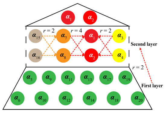
Figure 10.
The polynomial functional relationship between active modal coefficients where r represents the order of the library Θ(x). The α1 and α2 are active modal coefficients.
In the first layer, the functional relationship between most modes and a small part of modes is first constructed. This study found that all modal coefficients of these four airfoils can be represented by second-order polynomial functions of modal coefficients (α1, α2, α3, α4, α7, α8, α15, α16). The angular frequency corresponding to the active mode coefficient in the first layer is (ω, 2ω, 4ω, 8ω). When the second order is selected, the corresponding frequency of all modes can be covered. For the frequency relationship between the Seagull airfoil combined with the active mode coefficients and the Lissajous orbits, it is not difficult to see that the four pairs of active modes satisfy the following functional relationship:
when the second order is selected, the corresponding frequency of all modes can be covered.
The nonlinear correlation between the active modal coefficients is constructed in the second layer. In this study, there is only one pair of final active mode coefficients in airfoils, and the corresponding is the fundamental frequency of vortex shedding. Through the nonlinear correlation constructed by these two layers, the remaining modal coefficients can be accurately described by active modes (α1, α2). The nonlinear correlation between modal coefficients maps the frequency relationship between modes.
4.2. Manifold Dynamics and Flow Field Reconstruction
The nonlinear correlation of NACA4412, Ridged, Teal, and Seagull airfoils shows only one pair of active modes. The evolution of the modes of turbulent airfoils over time can be highly simplified as the modal coefficients of two degrees of freedom. The two-dimensional ordinary differential equations can approximate airfoil infinite-dimensional partial differential equations (ODEs, manifold equation). The manifold equation of Equation (13) was constructed based on SINDy, the one-order polynomial function library, and the FROLS. The four airfoils can construct the following two-dimensional manifold equation:
Whether a bionic airfoil or a NACA4412 airfoil, the constructed manifold equation has a unified form. The coefficients of the manifold equation correspond to the angular frequency of airfoil vortex shedding. The coefficients are opposite and the Lissajous orbit cycle indicates that the phase difference between the pair of modal coefficients is 90°.
The accuracy of flow field reconstruction is an essential criterion for verifying the accuracy of manifold equations. The active modal coefficients are first reconstructed using the manifold Equation (18). The remaining 18 modal coefficients are reconstructed from the nonlinear correlation (Figure 10). The modal and reconstructed modal coefficients are used for the final flow field reconstruction.
Figure 11 shows the effect of the reconstruction of the airfoil velocity field. The reconstructed velocity field based on the manifold equation at different times is highly consistent with the numerically simulated velocity field. The accuracy of the manifold equation and the fact that the minimum ROM is two-dimensional are revealed.

Figure 11.
Airfoil velocity field reconstruction based on manifold dynamics.
5. Conclusions
This study thoroughly explores the nonlinear correlation between the modal coefficients of Riblets, Seagull, and Teal airfoils and compares them with NACA4412. Based on the nonlinear correlation, a two-dimensional minimum ROM of the airfoil at an angle of attack of 19° was successfully constructed. The main conclusions are as follows:
- (1)
- The Seagull airfoil in the bionic airfoil has a more significant lift coefficient, while the Riblets has the smallest lift coefficient. The modes of airfoils are antisymmetric vortex-shedding structures. Under a large number of tiny serrations, the vortex-shedding structure in the middle of the upper surface of the Riblets airfoil disappears, and the high-frequency trailing edge vortex-shedding structure is different from the NACA4412 airfoil. The lift coefficient of the Teal airfoil is similar to the NACA4412 airfoil, but the vortex shedding frequency is significantly higher than the Seagull airfoil and the NACA4412 airfoil. The NACA4412, Riblets, and Seagull airfoil are mainly dominated by the trailing edge shedding vortex, while the Teal airfoil also includes the leading-edge LSB.
- (2)
- The first twenty DMD modes of the three airfoils are sufficient to ensure the accuracy of the velocity field reconstruction, and the spatial distribution of the modes is very similar. The mode frequency is multiple when the modal system is sorted by frequency. The relationship between the modal coefficients of the four airfoils is pure harmonic, and the shape is pure oscillation. The difference between modal coefficients is the difference between amplitude and phase. The phase difference between the paired modal coefficients is 90°, and the order of Lissajous orbits is conducive to building the specific function expression of nonlinear correlation.
- (3)
- The NACA4412, Riblets, Seagull, and Teal airfoil modal coefficients have the same type of nonlinear correlation, which is related to the frequency corresponding to the mode. The active mode has only a pair of active modes corresponding to the fundamental frequency. The rest of the modal coefficients can be represented by the active modes’ polynomial functions. The two-dimensional manifold equations constructed by the four airfoils are consistent, and the absolute value of the coefficient corresponds to the fundamental frequency of the airfoil vortex shedding. The flow field reconstructed based on manifold dynamics is in high agreement with the numerical simulation results, validating the accuracy of the simple, compact, and interpretable flow field equations.
Author Contributions
Conceptualization, Q.X. and J.W.; methodology, Q.X. and X.Y.; software, Q.X. and X.Y.; validation, X.Y., B.J. and J.W.; formal analysis, Q.X. and Y.D.; investigation, Q.X.; resources, Y.D. and B.J.; data curation, B.J. and X.Y.; writing—original draft preparation, Q.X.; writing—review and editing, Q.X. and X.Y.; visualization, Q.X. and X.Y; supervision, J.W. and Y.D.; project administration, B.J. and Y.D.; funding acquisition, Q.X. All authors have read and agreed to the published version of the manuscript.
Funding
This research was supported by the China Postdoctoral Science Foundation (Grant Number 2022M721238).
Data Availability Statement
The data presented in this study are available on request from the corresponding author. The data are not publicly available due to data occupying too much memory.
Acknowledgments
The authors thank the SCTS/CGCL HPCC of HUST for providing computing resources and technical support. The authors also appreciate all other scholars for their advice and assistance in improving this article.
Conflicts of Interest
The authors declare no conflict of interest.
References
- Aabid, A.; Parveez, B.; Parveen, N.; Khan, S.A.; Zayan, J.M.; Shabbir, O. Reviews on Design and Development of Unmanned Aerial Vehicle (Drone) for Different Applications. J. Mech. Eng. Res. Dev. 2022, 45, 53–69. [Google Scholar]
- Wright, A.K.; Wood, D.H. The starting and low wind speed behaviour of a small horizontal axis wind turbine. J. Wind Eng. Ind. Aerod. 2004, 92, 1265–1279. [Google Scholar] [CrossRef]
- Zhao, M.; Zhang, M.; Xu, J. Numerical simulation of flow characteristics behind the aerodynamic performances on an airfoil with leading edge protuberances. Eng. Appl. Comp. Fluid 2017, 11, 193–209. [Google Scholar] [CrossRef]
- Lewthwaite, M.T.; Amaechi, C.V. Numerical investigation of winglet aerodynamics and dimple effect of NACA 0017 airfoil for a freight aircraft. Inventions 2022, 7, 31. [Google Scholar] [CrossRef]
- Tian, H.; Shan, X.; Cao, H.; Xie, T. Enhanced performance of airfoil-based piezoaeroelastic energy harvester: Numerical simulation and experimental verification. Mech. Syst. Signal Process. 2022, 162, 108065. [Google Scholar] [CrossRef]
- Li, Z.; Shi, D.; Li, S.; Yang, X.; Miao, G. A systematical weight function modified critical distance method to estimate the creep-fatigue life of geometrically different structures. Int. J. Fatigue 2019, 126, 6–19. [Google Scholar] [CrossRef]
- Tripathi, D.; Vishal, S.; Bose, C.; Venkatramani, J. Stall-induced fatigue damage in nonlinear aeroelastic systems under stochastic inflow: Numerical and experimental analyses. Int. J. Nonlin. Mech. 2022, 142, 104003. [Google Scholar] [CrossRef]
- Plante, F.; Dandois, J.; Beneddine, S.; Laurendeau, É.; Sipp, D. Link between subsonic stall and transonic buffet on swept and unswept wings: From global stability analysis to nonlinear dynamics. J. Fluid Mech. 2021, 908, A16. [Google Scholar] [CrossRef]
- Akram, M.T.; Kim, M.H. Aerodynamic shape optimization of NREL S809 airfoil for wind turbine blades using reynolds-averaged navier stokes model—Part II. Appl. Sci. 2021, 11, 2211. [Google Scholar] [CrossRef]
- Jung, Y.S.; Vijayakumar, G.; Ananthan, S.; Baeder, J. Local correlation-based transition models for high-Reynolds-number wind-turbine airfoils. Wind Energy Sci. 2022, 7, 603–622. [Google Scholar] [CrossRef]
- Błoński, D.; Strzelecka, K.; Kudela, H. Vortex Trapping Cavity on Airfoil: High-Order Penalized Vortex Method Numerical Simulation and Water Tunnel Experimental Investigation. Energies 2021, 14, 8402. [Google Scholar] [CrossRef]
- Ma, A.; Gibeau, B.; Ghaemi, S. Time-resolved topology of turbulent boundary layer separation over the trailing edge of an airfoil. J. Fluid Mech. 2020, 891, 1–32. [Google Scholar] [CrossRef]
- Raheem, M.A.; Edi, P.; Pasha, A.A.; Rahman, M.M.; Juhany, K.A. Numerical study of variable camber continuous trailing edge flap at off-design conditions. Energies 2019, 12, 3185. [Google Scholar] [CrossRef]
- Zhao, M.; Zhao, Y.; Liu, Z. Dynamic mode decomposition analysis of flow characteristics of an airfoil with leading edge protuberances. Aerosp. Sci. Technol. 2020, 98, 105684. [Google Scholar] [CrossRef]
- Yuan, Y.; Yu, X.; Yang, X.; Xiao, Y.; Xiang, B.; Wang, Y. Bionic building energy efficiency and bionic green architecture: A review. Renew. Sust. Energ. Rev. 2017, 74, 771–787. [Google Scholar] [CrossRef]
- Lotfabadi, P.; Alibaba, H.Z.; Arfaei, A. Sustainability; as a combination of parametric patterns and bionic strategies. Renew. Sust. Energ. Rev. 2016, 57, 1337–1346. [Google Scholar] [CrossRef]
- Wang, T.; Wang, Z.; Zhang, B. Mechanism Design and Experiment of a Bionic Turtle Dredging Robot. Machines 2021, 9, 86. [Google Scholar] [CrossRef]
- Howe, M.S. Aerodynamic noise of a serrated trailing edge. J. Fluid Struct. 1991, 5, 33–45. [Google Scholar] [CrossRef]
- Avallone, F.; Van der Velden, W.C.P.; Ragni, D. Benefits of curved serrations on broadband trailing-edge noise reduction. J. Sound Vib. 2017, 400, 167–177. [Google Scholar] [CrossRef]
- Huang, X. Theoretical model of acoustic scattering from a flat plate with serrations. J. Fluid Mech. 2017, 819, 228–257. [Google Scholar] [CrossRef]
- Miklosovic, D.S.; Murray, M.M.; Howle, L.E.; Fish, F.E. Leading-edge tubercles delay stall on humpback whale (Megaptera novaeangliae) flippers. Phys. Fluid. 2004, 16, 39–42. [Google Scholar] [CrossRef]
- Hansen, K.L.; Kelso, R.M.; Dally, B.B. Performance variations of leading-edge tubercles for distinct airfoil profiles. AIAA J. 2011, 49, 185–194. [Google Scholar] [CrossRef]
- Rostamzadeh, N.; Hansen, K.L.; Kelso, R.M.; Dally, B.B. The formation mechanism and impact of streamwise vortices on NACA 0021 airfoil’s performance with undulating leading edge modification. Phys. Fluid. 2014, 26, 107101. [Google Scholar] [CrossRef]
- Srinivas, K.S.; Datta, A.; Bhattacharyya, A.; Kumar, S. Free-stream characteristics of bio-inspired marine rudders with different leading-edge configurations. Ocean Eng. 2018, 170, 148–159. [Google Scholar] [CrossRef]
- Kant, R.; Bhattacharyya, A. A bio-inspired twin-protuberance hydrofoil design. Ocean Eng. 2020, 218, 108209. [Google Scholar] [CrossRef]
- Chang, H.; Cai, C.; Li, D.; Zuo, Z.; Wang, H.; Liu, S. Effects of Reynolds Number and Protuberance Amplitude on Twin-Protuberance Airfoil Performance. AIAA J. 2022, 60, 3775–3788. [Google Scholar] [CrossRef]
- Pereira, L.T.L.; Ragni, D.; Avallone, F.; Scarano, F. Aeroacoustics of sawtooth trailing-edge serrations under aerodynamic loading. J. Sound Vib. 2022, 537, 117202. [Google Scholar] [CrossRef]
- Wang, L.; Liu, X.; Li, D. Noise reduction mechanism of airfoils with leading-edge serrations and surface ridges inspired by owl wings. Phys. Fluid. 2021, 33, 015123. [Google Scholar] [CrossRef]
- Li, D.; Chang, H.; Zuo, Z.; Wang, H.; Liu, S. Aerodynamic characteristics and mechanisms for bionic airfoils with different spacings. Phys. Fluid. 2021, 33, 064101. [Google Scholar] [CrossRef]
- Huang, S.; Hu, Y.; Wang, Y. Research on aerodynamic performance of a novel dolphin head-shaped bionic airfoil. Energy 2021, 214, 118179. [Google Scholar] [CrossRef]
- Liu, T.; Kuykendoll, K.; Rhew, R.; Jones, S. Avian wing geometry and kinematics. AIAA J. 2006, 44, 954–963. [Google Scholar] [CrossRef]
- Song, L.; Tian, K.; Jiao, X.; Feng, R.; Wang, L.; Tian, R. Design and optimization of seagull airfoil wind energy conversion device. Int. J. Green Energy 2021, 18, 1046–1063. [Google Scholar] [CrossRef]
- Li, D.; Liu, X. A comparative study on aerodynamic performance and noise characteristics of two kinds of long-eared owl wing models. J. Mech. Sci. Technol. 2017, 31, 3821–3830. [Google Scholar] [CrossRef]
- Huang, S.; Qiu, H.; Wang, Y. Aerodynamic performance of horizontal axis wind turbine with application of dolphin head-shape and lever movement of skeleton bionic airfoils. Energ. Convers. Manag. 2022, 267, 115803. [Google Scholar] [CrossRef]
- Zargar, O.A.; Lin, T.; Zebua, A.G.; Lai, T.J.; Shih, Y.C.; Hu, S.C.; Leggett, G. The effects of surface modification on aerodynamic characteristics of airfoil DU 06 W 200 at low Reynolds numbers. Int. J. Thermo. 2022, 16, 100208. [Google Scholar] [CrossRef]
- Mallik, W.; Raveh, D.E. Aerodynamic damping investigations of light dynamic stall on a pitching airfoil via modal analysis. J. Fluid. Struct. 2020, 98, 103111. [Google Scholar] [CrossRef]
- Schmid, P.J. Dynamic mode decomposition and its variants. Annu. Rev. Fluid Mech. 2022, 54, 225–254. [Google Scholar] [CrossRef]
- Naderi, M.H.; Eivazi, H.; Esfahanian, V. New method for dynamic mode decomposition of flows over moving structures based on machine learning (hybrid dynamic mode decomposition). Phys. Fluids 2019, 31, 127102. [Google Scholar] [CrossRef]
- Mohan, A.T.; Gaitonde, D.V. Analysis of airfoil stall control using dynamic mode decomposition. J. Aircr. 2017, 54, 1508–1520. [Google Scholar] [CrossRef]
- Tirandaz, M.R.; Rezaeiha, A. Effect of airfoil shape on power performance of vertical axis wind turbines in dynamic stall: Symmetric Airfoils. Renew. Energy 2021, 173, 422–441. [Google Scholar] [CrossRef]
- Callaham, J.L.; Brunton, S.L.; Loiseau, J.C. On the role of nonlinear correlations in reduced-order modelling. J. Fluid Mech. 2022, 938, A1. [Google Scholar] [CrossRef]
- Brunton, S.L.; Proctor, J.L.; Kutz, J.N. Discovering governing equations from data by sparse identification of nonlinear dynamical systems. Proc. Natl. Acad. Sci. USA 2016, 113, 3932–3937. [Google Scholar] [CrossRef] [PubMed]
- Sanei, M.; Razaghi, R. Numerical investigation of three turbulence simulation models for S809 wind turbine airfoil. Proc. Inst. Mech. Eng. Part A J. Power Energy 2018, 232, 1037–1048. [Google Scholar] [CrossRef]
- Winter, O.; Sváček, P. On numerical simulation of flexibly supported airfoil in interaction with incompressible fluid flow using laminar–turbulence transition model. Comput. Math. Appl. 2021, 83, 57–73. [Google Scholar] [CrossRef]
- Yang, X.; Wang, J.; Jiang, B.; Li, Z.A.; Xiao, Q. Numerical Study of Effect of Sawtooth Riblets on Low-Reynolds-Number Airfoil Flow Characteristic and Aerodynamic Performance. Processes 2021, 9, 2102. [Google Scholar] [CrossRef]
- Menter, F.R. Two-equation eddy-viscosity turbulence models for engineering applications. AIAA J. 1994, 32, 1598–1605. [Google Scholar] [CrossRef]
- Coles, D.; Wadcock, A.J. Flying-Hot-Wire Study of 2-Dimensional Mean Flow Past an NACA 4412 Airfoil at Maximum Lift. Bull. Am. Phys. Soc. 1978, 23, 991. [Google Scholar]
- Pinkerton, R.M. The Variation with Reynolds Number of Pressure Distribution over an Airfoil Section (No. NACA-TR-613); US Government Printing Office: Washington, WA, USA, 1938.
- Noack, B.R.; Afanasiev, K.; Morzyński, M.; Tadmor, G.; Thiele, F. A hierarchy of low-dimensional models for the transient and post-transient cylinder wake. J. Fluid Mech. 2003, 497, 335–363. [Google Scholar] [CrossRef]
- Loiseau, J.C.; Noack, B.R.; Brunton, S.L. Sparse reduced-order modelling: Sensor-based dynamics to full-state estimation. J. Fluid Mech. 2018, 844, 459–490. [Google Scholar] [CrossRef]
- Rowley, C.W.; Mezić, I.; Bagheri, S.; Schlatter, P.; Henningson, D.S. Spectral analysis of nonlinear flows. J. Fluid Mech. 2009, 641, 115–127. [Google Scholar] [CrossRef]
- Cai, Z.; Dang, Z.; Wen, M.; Lv, Y.; Duan, H. Application of Compressed Sensing Based on Adaptive Dynamic Mode Decomposition in Signal Transmission and Fault Extraction of Bearing Signal. Machines 2022, 10, 353. [Google Scholar] [CrossRef]
- Gibeau, B.; Koch, C.R.; Ghaemi, S. Active control of vortex shedding from a blunt trailing edge using oscillating piezoelectric flaps. Phys. Rev. Fluid. 2019, 4, 054704. [Google Scholar] [CrossRef]
- Lopez-Paz, D.; Hennig, P.; Schölkopf, B. The randomized dependence coefficient. Adv. Neural Inf. Process. Syst. 2013, 26, 1–9. [Google Scholar]
- Rudy, S.H.; Brunton, S.L.; Proctor, J.L.; Kutz, J.N. Data-driven discovery of partial differential equations. Sci. Adv. 2017, 3, 3932–3937. [Google Scholar] [CrossRef] [PubMed]
- Loiseau, J.C. Data-driven modeling of the chaotic thermal convection in an annular thermosyphon. Theor. Comp. Fluid Dyn. 2020, 34, 339–365. [Google Scholar] [CrossRef]
Disclaimer/Publisher’s Note: The statements, opinions and data contained in all publications are solely those of the individual author(s) and contributor(s) and not of MDPI and/or the editor(s). MDPI and/or the editor(s) disclaim responsibility for any injury to people or property resulting from any ideas, methods, instructions or products referred to in the content. |
© 2023 by the authors. Licensee MDPI, Basel, Switzerland. This article is an open access article distributed under the terms and conditions of the Creative Commons Attribution (CC BY) license (https://creativecommons.org/licenses/by/4.0/).