Abstract
Rapid changes in the performance-related parameters of a pump during its startup operation lead to large pressure fluctuations and structural vibrations in it. In view of these problems, this study investigates the evolution of cavitation and the characteristics of fluctuations under pressure in a centrifugal pump during startup. We use the finite volume method to simulate this dynamic process. To characterize the acceleration, we assume that the rotational speed and rate of flow of the pump are not constant but vary with time. A steady-state numerical simulation is performed to examine the external characteristics of the pump to verify the accuracy of the numerical procedure. The evolution of fluctuations in the cavity and pressure over time is then analyzed in detail. We use the short-term Fourier transform for post-processing in light of its advantage in treating non-stationary signals. The results indicate that both the frequency and the amplitude of the fluctuations in pressure increase with the speed of the impeller. The transient operation causes the average pressure at the inlet of the impeller to decrease to the evaporation pressure, and this leads to an increase in the volume fraction of vapor. Moreover, both the impeller–tongue interaction and the impeller–diffuser interaction influence the fluctuations in cavitation.
1. Introduction
Centrifugal pumps are widely used in energy-related applications and chemical engineering. Owing to the growing demand for a large amount of reliable sources of power as well as the increasing complexity of the systems used in chemical engineering, the transient operations (the processes of startup, termination, and variations in speed) of centrifugal pumps have received considerable attention in research in the past few decades. Its performance-related parameters (such as the rotational speed, rate of flow, and total head) undergo rapid variations over a short period during startup, where this induces large fluctuations in the pressure and vibrations of the pumps. Therefore, many researchers have investigated the characteristics of the centrifugal pump during its transient operations.
Experimental and theoretical methods were used in early work in the area. In the 1980s, Grover and Koranne [1] developed the first computer program to theoretically investigate the startup process of the pump. Tsukamoto et al. [2,3] theoretically and experimentally studied the transient characteristics of a centrifugal pump during its rapid acceleration and deceleration. They showed that a non-dimensional head was significantly different from one operating under the assumption of a quasi-steady state, where this provided a new avenue for research on the transient operation of pumps. Lefebvre and Barker [4] also pointed out that the assumption of a quasi-steady state was not valid in the case of highly transient (acceleration or deceleration) operations. Thanapandi and Prasad [5] proposed a theoretical model that was useful for analyzing transient operations, especially in the case of a large departure of the dynamic parameters from the steady state.
In addition to experimental and theoretical methods, many researchers now use computational fluid dynamics (CFD) to analyze the characteristics of the performance of the pump during transient operations. Zhang [6] established a closed-loop piping system containing the model of a centrifugal pump to study its startup process, and solved its transient flow through numerical self-coupling computations without specifying any boundary condition to eliminate errors introduced by externally prescribed unsteady boundary conditions. Li et al. [7] used CFD to investigate the relationship between the evolution of transient flow and the corresponding instantaneous rates of flow, head, efficiency, and power during a rapid startup period by using a self-coupling model. Liu et al. [8] subsequently used the same method to investigate the rapid stopping process of a centrifugal pump. Wu et al. [9] numerically studied the unsteady flow field in a centrifugal pump by considering the opening of the discharge valve. They claimed that the evolution of the vortex and the acceleration of the fluid primarily influence the performance of the pump. In the context of chemical engineering, Singh et al. [10] investigated the baffle–impeller interaction of the pump mixer by using single-phase CFD.
Due to limitations in the layout of their pipeline, the inlet of some feedwater pumps is short of pressure-supply pumps, because of which pressure at their inlet is lower than normal. As it begins pumping, potential energy in the pump is transformed into kinetic energy such that its local pressure is lower than the saturated pressure of steam, and this can easily cause cavitation. Cavitation is unavoidable during the transient operation of a pump under this condition. Some important reviews of cavitation in hydraulic machinery had been provided in the literature. Brennen described the compliance and gain in mass flow of the pump, which was critical to its stability as well as that of the overall system [11]. Luo reviewed the latest progress in research on cavitation in hydraulic machinery and the relevant problems by simulating cavitation-induced turbulence in centrifugal pumps, axial flow pumps, and turbines [12]. Some researchers have focused on the excitation of fluctuations in pressure due to cavitation. Ji studied the relationship between the fluctuations in pressure around a hydrofoil and the cavity-shedding process, and the results indicated that the accelerated growth of the volume of the cavity was the main source of fluctuations in pressure around the cavitation in a hydrofoil [13]. Ji confirmed the effect of an inclined propeller in terms of reducing vibrations and noise by simulating the cavitation flow of two marine propellers with different inclination angles (an ordinary propeller and a high-tilt propeller) in a non-uniform wake [14]. Peng et al. established a model of cavitation induced by the compressible mixed flow of bubbles that can be used to calculate turbulent cavitation-induced flow, and can adequately capture the unstable shedding of the cavitation cloud while providing the means to observe it [15]. Zima et al. proposed and verified a method to accurately determine the main frequencies of oscillations in cavitation structures to observe the subtle characteristics of flow [16].
Some researchers have focused on cavitation–vortex interactions. Ji et al. accurately identified the vortex-shedding structure of the wake of the cavitation of a hydrofoil when examining turbulent adhesion-based cavitation flow around the Clark-Y hydrofoil, and found that fluctuations in the turbulent velocity of large structures were affected by cavitation-shedding [17]. Ji et al. conducted numerical simulations of the structure of the cavitation-induced flow in a twisted hydrofoil, analyzed the flow on its suction side, and found that cavitation promoted the generation of vorticity that led to a local separation and unstable flow [18]. Tanaka and Tsukamoto [19,20,21] used a high-speed camera to visualize the behavior of the cavity during transient operations in a centrifugal pump. They found that fluctuations in the instantaneous pressure and flow were influenced by both oscillations in the cavitation and the separation of the water column. More recently, Wu et al. [22] performed experiments under various conditions and found that cavitation in the startup process can lead to a significant degradation in performance and fluctuations in the head. They concluded that cavitation can be delayed by accelerating the flow. Dulpaa et al. [23,24,25] experimentally studied different startup behaviors under conditions of cavitation. They observed a water hammer phenomenon at the inlet and the outlet of the pump. Following them, Meng [26] proposed a Fluent–Flowmaster method of coupling to simulate cavitation during startup, and successfully predicted fluctuations in pressure in the fluid domain under transient operation.
As shown above, past work on cavitation in centrifugal pumps during their startup operations had mostly focused on their external characteristics through experimental examinations. Because the dynamic evolution of the fluctuations in pressure and cavitation within the flow are more complex and have been scarcely investigated, detailed information on the phenomena inside the pump is not available. We thus use the finite volume method in this study to numerically investigate the fluctuations in pressure and cavitation during the startup process of the pump in order to obtain a better insight into such transient phenomena. We first numerically validate the external characteristics of the pump in a steady state. Following this, we analyze the processes of evolution of cavitation (generation, evolution, and distribution) and the fluctuations in pressure in different domains under two values of the suction pressure during the startup of the pump.
2. Materials and Methods
The startup process is simulated by using CFD code in ANSYS FLUENT. In order to characterize the dynamic characteristics of the pump, its speed of rotation and rate of flow is no longer assumed to be constant but vary with time. The subroutines are embedded by a user-defined function to characterize the non-constant speed of rotation of the impeller and the transient boundary conditions of the pump unit. Moreover, because signals of the static pressure (unless otherwise stated, the pressure examined is static pressure) during the startup period constitute a non-stationary time series, the spectrum of amplitude obtained by the fast Fourier transform (FFT), the most commonly used method for time–frequency representation, is complex and all the temporal information was lost. To further examine the temporal history of the components of frequency during the entire startup period, we use the short-term Fourier transform (STFT), which is an effective method for time–frequency analysis.
2.1. Computational Domain and Mesh System
A single-stage centrifugal pump is investigated here. The pump is an in-house designed centrifugal pump. Its structure and a diagram of the structural explosion are shown in Figure 1. It consists of four parts: (a) inlet guide vanes with three blades to improve the pattern of flow in the inlet of tkhe impeller, leading to a more uniform distribution of pressure; (b) an impeller composed of five backward blades and five additional splitter blades, a unique design that could increase the area of flow at the inlet of the impeller; (c) diffuser vanes with seven blades to collect the liquid thrown from the impeller and smoothly guide it into the volute; and (d) a volute to convert kinetic energy into static pressure-induced energy, and to guide the liquid toward the outlet. Extended pipes are added to the inlet and outlet of the domain to ensure the full development of the state of flow. A 3D perspective of the model pump is shown in Figure 2, and other performance-related and geometric parameters are listed in Table 1.
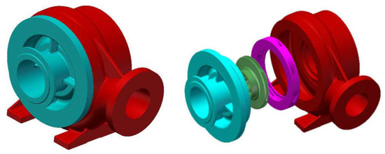
Figure 1.
Structural diagram of the model and its structural explosion diagram.
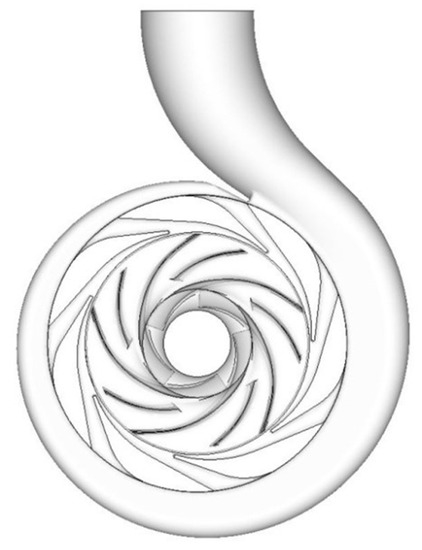
Figure 2.
3D perspective of the region of the fluid.

Table 1.
Specifications of the test section.
Given the complexity of the volute, a mesh is generated by the tetrahedral method to make it adequately adaptable, and hexahedral mesh systems are used for the other regions. The boundary layer is refined for flow separation and pressure gradients. The grid is stretched away from the solid wall boundary, where this constitutes a suitable compromise between points on the mesh and the computational cost. The use of the turbulence model requires a specific range of the wall variable (where y is the wall-normal distance of the closest grid to the wall, is kinematic viscosity, and is the frictional velocity, with and the shear stress of the wall and the density of the fluid, respectively).
For the grid independence test, we use the RNG turbulence model, and set its primary phase to water and secondary phase to water vapor. The Schnerr–Sauer cavitation model is used, the number density of the bubbles is 1 × 10¹³, and the cavitation pressure is 3540 Pa. A constant pressure of 0.1 MPa is applied at the inlet. The boundary condition is a transient rate of mass flow at the outlet, and is set to a cubic profile that corresponds to the opening of the regulating valve. The final rate of mass flow is 16.4 kg/s.
The inlet, the inlet guide vane, the volute, and the outlet are set as static areas in the software. The impeller is the rotating area, and its speed is set to 2980 r/min. The sliding grid model is used to solve the transient state. The value of of the wall is varied from 30 to 300 in the RNG turbulence model. The values of of the impeller and the volute in the pump are shown in Figure 3, and satisfy the requirements of the turbulence model. Seven grid schemes, ranging from 1 million to 4.6 million grids, are designed, and transient calculations are performed to obtain the value of the head. Figure 4 shows that when the total number of grids is 2.56 million, the increase in the number of grids makes little contribution to the convergence of the head. After comprehensive consideration, a model with 2.56 million grids is selected for use. The detailed mesh of the region of the fluid is shown in Figure 5.
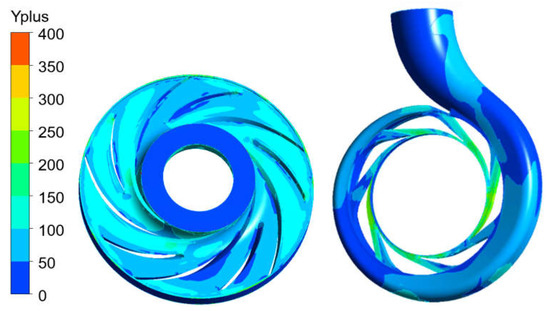
Figure 3.
values of the impeller and the area of the volute.
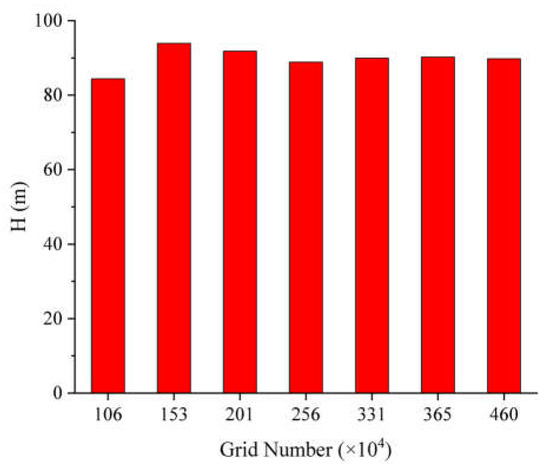
Figure 4.
Analysis of independence of grids of the mesh.
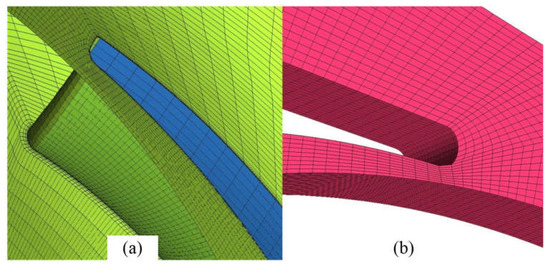
Figure 5.
Surface mesh of the impeller: (a) leading edge and (b) trailing edge.
The non-dimensional pressure coefficient Cp is defined in the following equations: Cp = 2p/(ρu2). Where p and u are pressure and the tangential speed of the impeller. Time-step independence analysis is an indispensable step in unsteady flow simulation. The transient pressure (excluding the mean pressure) at the pump outlet is shown in Figure 6. The duration of the impeller passing 1° is 5.593 × 10⁻⁵ s, which corresponds to 1 basic unit. Four-time steps ranging from 0.5 base unit to 4 base unit are chosen. Pressure changes are negligible when the time step is less than 1 base unit. Therefore, considering the computation time and accuracy, we set the time step as 5.593 × 10⁻⁵ s.

Figure 6.
Time-step independence analysis.
2.2. Governing Equations
We use a homogeneous multi-phase model that has been widely used for cavitating flows to simulate the characteristics of cavitation in the centrifugal pump. The equations of continuity and momentum are as follows:
where u represents the velocity vector, g is gravitational acceleration, and P denotes the pressure of the flow field. (), () and are the density of the mixture, its dynamic viscosity, and the volume fraction of vapor, respectively. represents the ratio of the volume of steam in the fluid domain to the volume of the grid.
Given the two-phase large-scale flow separation, the RNG model [27] (flow with a high streamline curvature and a high strain rate can be accurately modeled by the RNG turbulence model) together with the standard wall function [28] are used for the closure of turbulence. The wall functions use the predictable dimensionless profile of the boundary layer to allow conditions at the wall (e.g., shear stress) to be determined according to whether the centroid of the cell of the mesh adjacent to the wall is located in the log-layer, and to locate the first cell in the log-layer. The variable of the wall varies from 30 to 300 in the RNG turbulence model [29]. To estimate as a function of a desirable value of , we use a truncated series solution of the Blasius equation [30]:
where is the mean velocity at the inlet, and the reference length, , is the distance between the curves of the hub and the shroud upstream of the first row of the blade. This is an approximation, of course, because the thickness of the boundary layers varies widely within the computational domain. It is only necessary to place within a specified range instead of at a certain value. The range of indicates that the near-wall nodes are within the laminar sublayer.
2.3. Cavitation Model
We use the Schnerr–Sauer cavitation model [31], which has been validated for many cases involving cavitation [32,33]. We have also used it in past work [34,35]:
where and represent the rates of evaporation and condensation of vapor, respectively.
In the above, denotes the diameter of the bubble, , (recommended by Schnerr and Sauer [31]), and represents the saturation pressure.
2.4. Numerical Method and Conditions
The calculated region is divided into a dynamic and a static region. The dynamic mesh method combined with non-conformal grid boundaries are used to simulate the rotation of the impeller. During the startup process, the region of fluid of the impeller accelerated as a whole. A pair of interfaces is imposed for the relative motion of the rotation and the stationary regions, as shown in Figure 7. Data exchange between the rotor and the stator is carried out by using an interpolation routine.
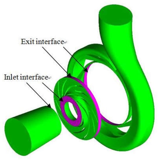
Figure 7.
Grid interfaces at the inlet and exit of the impeller.
The duration of acceleration of the impeller, pressure at the inlet, and opening of the outlet-regulating valve are the three main operating parameters during the startup process. The impeller accelerates exponentially from a stationary state to its final condition, and the temporal evolution of its speed of rotation is calculated by the following time-dependent equation:
where the final speed of rotation r/min, and t0 is the time constant of acceleration that is set to 0.15 s, and is related to the increase in the speed of the impeller to 63.2% of its final speed. Constant pressure is imposed at the inlet, and its values are set to 20 and 50 kPa for two cases. The boundary condition is the transient rate of mass flow at the outlet, and is set to a cubic profile corresponding to the opening of the regulating valve. The final rate of mass flow is 16.4 kg/s (as shown in Table 2). The laws of dynamic changes in the speed of rotation and the mass flow rate are both obtained through experiments [36].
Table 2.
Two startup conditions.
A coupled algorithm is used to solve the pressure–velocity coupling. It is robust and converges quickly, particularly for cavitation flows in rotating machinery [29]. The pressure and velocity fields are discretized by PRESTO! and the second-order upwind scheme, respectively. The time step is set to 5.593 × 10⁻⁵ s, which is approximately the time taken for the rotor to rotate by 1° at its final, constant speed of rotation. The maximum number of iterations is 200 for each time step.
3. Results
The external characteristics of the two cases in the final steady state are first numerically validated. Table 3 shows that the numerical results agreed well with the experimental data. All subsequent analyses are conducted for the dynamic startup process.
Table 3.
Comparison between the experimental results and those of CFD.
3.1. Evolution of Cavitation during the Startup Process
Figure 8 shows the time histories of the speed of rotation, mass flow rate, and total head during the startup process under two conditions. It is clear that the average total head rose overall, with a tendency similar to that of the speed of rotation. Moreover, the fluctuation in the amplitude of the dynamic head increases as the impeller accelerated. The average head in Case 1 is lower than that in Case 2 during the entire startup process, in accordance with the different boundary conditions used.
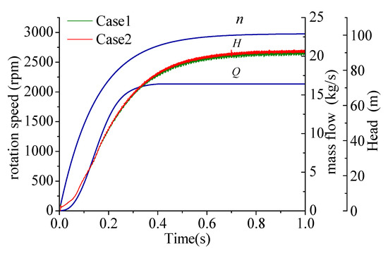
Figure 8.
Curves of the speed of rotation, mass flow rate, and total head vs. time.
Figure 9 plots the rates of change in the speed of rotation, mass flow rate, and total head. The time derivative of the speed of rotation declines rapidly to a stable value during the startup process. The rate of change in the flow of mass increases to its maximum at 0.15 s and then fell gradually but remains positive from 0.15 s to 0.4 s, indicating that it had slowed down. At 0.4 s, the rate of flow reaches a steady state and remains stable during the remaining time. At t < 0.1 s, the rate of change in the total head remains almost constant and variations in the head are not evident; during 0.1–0.4 s, the curve exhibited prominent fluctuations that become more intense with the acceleration of the impeller; when t is above 0.4 s, the amplitude of fluctuations remains stable. This analysis shows that the transient boundary conditions have a significant impact on the external characteristics of the pump during the startup period.

Figure 9.
Rate of change in the external characteristics during the startup process.
The distribution of pressure at the mid-span of the impeller is shown in Figure 10. Given that it has the same trend in both cases, only the results of Case 1 are shown. The pressure throughout the volute increases rapidly during the startup process. The low-pressure region gradually shrinks toward the inlet of the impeller, and this corresponded to the evolution of cavitation. Figure 11 shows the overall development of the distribution of cavitation in the two cases. In Case 1, cavitation first appears at the leading edge of the suction side of the blades at 0.05 s. With the acceleration of the impeller, the cavitation zone gradually extends downstream toward the trailing edge of the impeller. From 0.05 to 1 s, bubbles are rapidly formed and lead to severe cavitation. The development of cavitation in Case 2 is similar to that in Case 1. However, the bubbles in Case 2 first appear at 0.1 s, later than in Case 1. They fill the inlet channel of the impeller in Case 1 such that cavitation is more severe than in Case 2 and reduces the working capacity of the impeller. The lower pressure at the inlet results in more significant cavitation, subsequently leading to a progressive drop in the head of the pump as described above. in Figure 11 is the ratio of the volume of vapor to the overall volume of the grid.
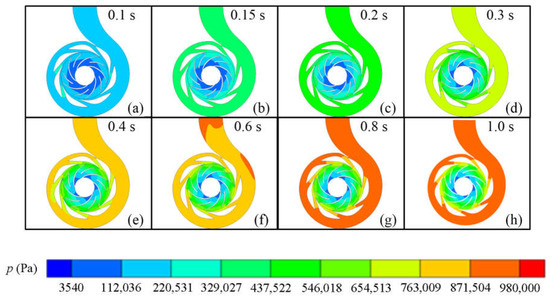
Figure 10.
Schematic diagram of the pressure distribution during the startup process: (a) t = 0.1 s (b) t = 0.15 s (c) t = 0.2 s (d) t = 0.3 s (e) t = 0.4 s (f) t = 0.6 s (g) t = 0.8 s (h) t = 1.0 s.
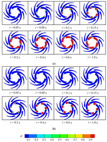
Figure 11.
Development of cavitation: (a) Case 1 and (b) Case 2.
Figure 12b shows the time histories of the volume fraction of vapor in the impeller domain in the two cases. The volume fraction of vapor is the percentage of the volume of cavitation in the impeller occupying the volume of the fluid domain in it. The developmental tendencies of the vapor are similar in the two cases. The overall trend of the curves of both increases gradually and stabilizes as the speed of the impeller increase. To obtain more details on cavitation, the last five revolutions (0.9–1 s) are selected for further analysis. Periodic fluctuations in the volume fraction of vapor are clear in the enlarged view (Figure 12a). The cycle of fluctuations lasts exactly 0.02 s, corresponding to the period of rotation. Moreover, higher-frequency fluctuations occur during one cycle of rotation. There are five peaks in one cycle, corresponding to the number of blades of the impeller.
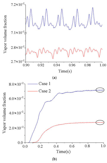
Figure 12.
Time histories of the volume fraction of vapor in the impeller domain: (a) the enlarged view; (b) the focused view.
Fluctuations in the volume of vapor are driven by those in the pressure of the flow field. We thus analyze the fluctuations in pressure during the startup process to investigate the internal causes of the development of cavitation.
3.2. Analysis of Fluctuations in Pressure
The model pump is composed of an impeller, inlet vanes, and diffuser vanes. The fluctuations in pressure within the pump are influenced by the combined interaction of the three components.
To obtain data on the pressure during the startup process, several monitoring points are positioned in the flow domain as shown in Figure 13. Points bp1 and bs1 are located in the cavitation zone on the pressure side and the suction side, respectively, points bs2 and bp2 are located in the middle of the blade, and points bs3 and bp3 are at the exit of the impeller. To ensure accuracy, the monitoring points in this domain are set to rotate with the impeller. Points G1–G3 are located at one of the seven passages of the diffuser vane along the streamline, and points V0–V5 are located in the middle of the cross-section of the volute along the streamline from the tongue to the exit.
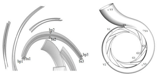
Figure 13.
Location of the monitoring points in the flow domain.
The fluctuations in pressure at bs1–bs3 and bp1–bp3 are shown in Figure 14. The curves exhibited two tendencies. The average pressure at bs1 and bp1 decrease to the evaporation pressure of 3540 Pa at 0.2 s and 0.05 s, respectively. The pressure remains constant during the remainder, and corresponded to the evolution of the cavity, while the average pressure in the middle of the blade and the exit gradually increases to stable values, exhibiting the same tendency as is observed with the acceleration of the impeller.

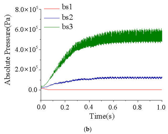
Figure 14.
Pressure along the direction of flow of the passage of the blade: (a) on the pressure side, and (b) on the suction side.
To better understand the process, the last five rotation cycles are selected to analyze the fluctuations in pressure (Figure 15). The amplitude of pressure exhibits a modulated pattern that is characterized by the presence of seven maxima and minima per rotation, and corresponds to the number of blades of the diffuser. In addition to high-frequency signals of fluctuation, lower-frequency signals are also observed, especially at bs2 on the suction side.
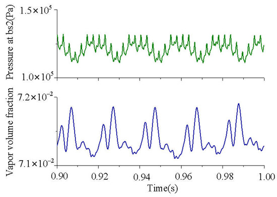
Figure 15.
Pressure at bs2 and volume fraction of vapor at the impeller at 0.9–1.0 s.
This modulation phenomenon can be attributed to the combined effect of the diffuser vanes and the volute as follows: (a) The stator–rotor interaction between the impeller and the diffuser vane results in high-frequency fluctuations with seven peaks per rotation, where this can explain similar high-frequency fluctuations in the volume fraction of vapor shown above. (b) The impeller–tongue interaction occurred in the pressure field. The monitoring point rotates with the impeller and, thus, is affected by the pressure distribution in the volute and changes in pressure with the distance from the tongue. The pressure decreases as the blade moves closer to the tongue, and this generates fluctuations in pressure with a rotation cycle of 0.02 s.
The development of cavitation is driven by the change in pressure, because of which the volume fraction of vapor fluctuates with the same period as the pressure. The volume fraction of vapor increases with the reduction in pressure. The above analysis indicates that the change in pressure in the impeller is the internal cause of the development of cavitation.
The spectrum of the amplitude of fluctuations in pressure obtained at the impeller is shown in Figure 16. Because the pressure signals during startup form a non-stationary time series, the spectrum of the amplitude obtained by FFT is complex and contains multiple groups of frequencies. Zigzag fluctuations are observed between crests. To further examine the time history of the components of frequency during the entire startup process, we conduct a time–frequency analysis.
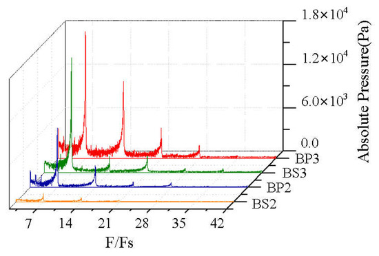
Figure 16.
Spectrum of the amplitude of fluctuations in pressure at the impeller.
The STFT is an effective method for time–frequency analysis. The basic idea is to use a fixed and a moving window to analyze non-stationary signals under the assumption that the signal in each window is stationary. The Hamming window is used, and the length of the window is set to 128 × 10−3 s.
Figure 17 shows the time–frequency characteristics of pressure at the impeller, plotted according to the duration and frequency of flow. The frequency is normalized by the final rotational frequency Fs, which was 50 Hz. The color bar indicates the level of pressure. The formula for this is , where A is the pressure (dB) and P is the pressure at the monitoring point (Pa). The dominant component of frequency in the spectrum corresponded to seven times the rotational frequency, and is the blade-passing frequency of the diffuser. The other components appear at the rotational frequency and higher harmonics of the blade-passing frequency of the diffuser, where this is consistent with the above analysis. As the impeller accelerates, all the components of frequency gradually increase, and have the same tendency as the speed of rotation. Moreover, the pressure at bp3 and bs3 are significantly higher than those at bp2 and bs2, indicating that the fluctuations in the impeller become more intense along the direction of flow.
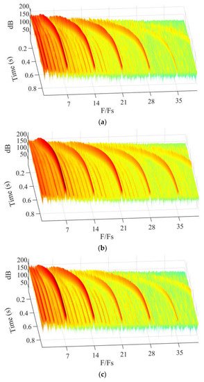
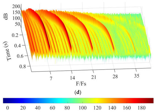
Figure 17.
Time–frequency characteristics of pressure at the impeller: (a) bp2, (b) bp3, (c) bs2, and (d) bs3.
The time history of pressure at the inlet guide vanes is shown in Figure 18. In the beginning, the average pressure gradually decreases and reaches its minimum value at 0.15 s due to the effect of inertia. Then, as the impeller rotates, the pressure gradually rebounds and stabilizes. The fluctuations in pressure at S1 are not prominent because it is far from the impeller.

Figure 18.
Development of pressure at the inlet guide vane.
The fluctuations in pressure at G1–G3 are shown in Figure 19, and correspond to the locations of the inlet, middle, and outlet of the diffuser guide vane, respectively. It is clear that the pressures at the three monitoring points are initially nearly the same. As the pump starts, the average pressure in the diffuser guide vanes gradually increases from upstream to downstream, indicating that the guide vanes have further converted kinetic energy into static pressure.
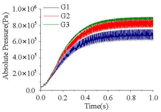
Figure 19.
Development of pressure at the diffuser.
Time–frequency analysis is carried out at G1–G3 as shown in Figure 20. The dominant components of frequency are also the BPFs and the higher harmonics of the BPF, where this can be attributed to the impeller–diffuser interaction. The components of frequency all increase with the startup of the pump. Meanwhile, both the number and the pressure level of the characterized frequency gradually decrease from G1 to G3, which indicates that the fluctuations in pressure characteristics gradually weaken along the flow direction.
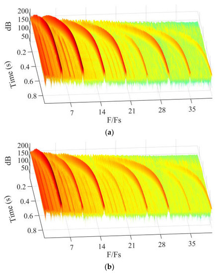
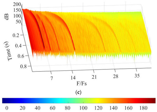
Figure 20.
Time–frequency characteristics of pressure at the diffuser vane: (a) G1, (b) G2, and (c) G3.
Figure 21 shows the time histories of the monitoring points on the volute. The fluctuations in pressure at the six locations are almost the same. Figure 21b shows an enlarged view of the last period of rotation, in which frequency modulation can be observed. Therefore, we use the point at the tongue, V0, as an example to extract the components of frequency in the pressure signals. The results are shown in Figure 22. The main components of frequency in the volute are five times (BPF), seven times (the passing frequency of the diffuser vane), and 15 times the rotational frequency. The flow moving into the volute is influenced by both the impeller and the diffuser vane, because of which fluctuations in the volute are caused by the combined effect of the impeller and the diffuser vane.
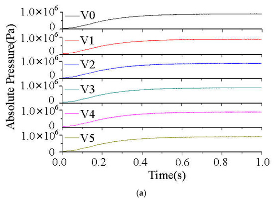
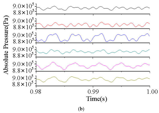
Figure 21.
Development of pressure at the volute: (a) the focused view and (b) the enlarged view.
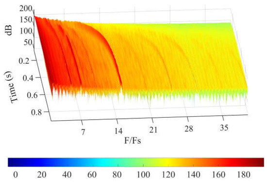
Figure 22.
Time–frequency characteristics of pressure at the volute.
4. Discussion
In this paper, the authors numerically investigate the dynamic operation of a centrifugal pump during the startup period. The evolution of cavitation and fluctuations in pressure are analyzed in detail. The following conclusions can be drawn:
(1) During the startup period, pressure in the pump exhibits prominent transient characteristics, and the overall trend of the average pressure is influenced by the transient operating conditions. Both the frequency and the amplitude of fluctuations in pressure increase with the acceleration of the impeller. The STFT effectively captures the non-stationary characteristics of pulsations in pressure during the startup of the pump.
(2) The time derivative of the speed of rotation declines rapidly to a stable value. The rate of change in the mass flow rate increased to a maximum and then fell gradually but still remained positive, indicating that it has slowed down. The rate of change in the total head remains almost constant, then fluctuates prominently, and becomes more intense as the impeller accelerates. When a sufficiently long time has passed, the amplitude of fluctuation remains stable. The transient boundary conditions have a significant impact on the external characteristics of the pump.
(3) Three factors influence the evolution of cavitation in the pump during the startup period. Transient operating conditions cause the average pressure at the inlet of the impeller to decrease to the evaporation pressure, and the volume fraction of vapor gradually increases. The impeller–tongue interaction, caused by the rotation of the impeller, results in fluctuations in the volume fraction of vapor with the rotational frequency. The impeller–diffuser interaction leads to high-frequency fluctuations in the volume fraction of vapor within a period of rotation.
Author Contributions
Conceptualization, S.L. and G.Z. Data curation, S.L. and H.C. Formal analysis, G.Z. Funding acquisition, C.J. Investigation, S.L. and H.C. Methodology, S.L. Project administration, G.Z. Resources, Y.C. Supervision, G.Z. Validation, S.L., H.C., Y.C. and S.N. Visualization, H.C. Writing–original draft, S.L. Writing—review and editing, S.L. All authors have read and agreed to the published version of the manuscript.
Funding
This research was funded by the National Natural Science Foundation of China (Grant No. 52241101).
Data Availability Statement
The data that support the findings of this study are available from the corresponding authors upon reasonable request.
Acknowledgments
We would like to thank the editors and the reviewers for their constructive comments and helpful suggestions.
Conflicts of Interest
The authors declare no conflict of interest.
References
- Grover, R.B.; Koranne, S.M. Analysis of pump start-up transients. Nucl. Eng. Des. 1981, 67, 137–141. [Google Scholar] [CrossRef]
- Tsukamoto, H.; Ohashi, H. Transient characteristics of a centrifugal pump during starting period. J. Fluids Eng. 1982, 104, 6–13. [Google Scholar] [CrossRef]
- Tsukamoto, H.; Matsunaga, S.; Yoneda, H.; Hata, S. Transient characteristics of a centrifugal pump during stopping period. J. Fluids Eng. 1986, 108, 392–399. [Google Scholar] [CrossRef]
- Lefebvre, P.J.; Barker, W.P. Centrifugal pump performance during transient operation. J. Fluids Eng. 1995, 117, 123–128. [Google Scholar] [CrossRef]
- Thanapandi, P.; Prasad, R. Centrifugal pump transient characteristics and analysis using the method of characteristics. Int. J. Mech. Sci. 1995, 37, 77–89. [Google Scholar] [CrossRef]
- Zhang, Y. Transient Internal Flow and Performance of Centrifugal Pumps during Startup Period. Ph.D. Thesis, Zhejiang University, Hangzhou, China, 2013. (In Chinese). [Google Scholar]
- Li, Z.; Wu, D.; Wang, L.; Huang, B. Numerical simulation of the transient flow in a centrifugal pump during starting period. J. Fluids Eng. 2010, 132, 081102. [Google Scholar] [CrossRef]
- Liu, J.; Li, Z.; Wang, L.; Jiao, L. Numerical simulation of the transient flow in a radial flow pump during stopping period. J. Fluids Eng. 2011, 133, 111101. [Google Scholar] [CrossRef]
- Wu, D.; Wu, P.; Li, Z.; Wang, L. The transient flow in a centrifugal pump during the discharge valve rapid opening process. Nucl. Eng. Des. 2010, 240, 4061–4068. [Google Scholar] [CrossRef]
- Singh, K.K.; Mahajani, S.M.; Shenoy, K.T.; Patwardhan, A.W.; Ghosh, S.K. CFD modeling of pilot-scale pump-mixer: Single-phase head and power characteristics. Chem. Eng. Sci. 2007, 62, 1308–1322. [Google Scholar] [CrossRef]
- Brennen, C.E. A review of the dynamics of cavitating pumps. J. Fluids Eng. 2013, 135, 061301. [Google Scholar] [CrossRef]
- Luo, X.; Bin, J.I.; Tsujimoto, Y. A review of cavitation in hydraulic machinery. J. Hydrodyn. Ser. B 2016, 28, 335–358. [Google Scholar] [CrossRef]
- Ji, B.; Luo, X.W.; Arndt, R.E.; Peng, X.; Wu, Y. Large eddy simulation and theoretical investigations of the transient cavitating vortical flow structure around a NACA66 hydrofoil. Int. J. Multiph. Flow 2015, 68, 121–134. [Google Scholar] [CrossRef]
- Ji, B.; Luo, X.; Wu, Y. Unsteady cavitation characteristics and alleviation of pressure fluctuations around marine propellers with different skew angles. J. Mech. Sci. Technol. 2014, 28, 1339–1348. [Google Scholar] [CrossRef]
- Peng, G.; Yang, C.; Oguma, Y.; Shimizu, S. Numerical analysis of cavitation cloud shedding in a submerged water jet. J. Hydrodyn. Ser. B 2016, 28, 986–993. [Google Scholar] [CrossRef]
- Patrik, Z.I.M.A.; Fürst, T.; SedláŘ, M.; Komárek, M.; Huzlík, R. Determination of frequencies of oscillations of cloud cavitation on a 2-D hydro-foil from high-speed camera observations. J. Hydrodyn. Ser. B 2016, 28, 369–378. [Google Scholar]
- Ji, B.; Long, Y.; Long, X.P.; Qian, Z.D.; Zhou, J.J. Large eddy simulation of turbulent attached cavitating flow with special emphasis on large scale structures of the hydrofoil wake and turbulence–cavitation interactions. J. Hydrodyn. Ser. B 2017, 29, 27–39. [Google Scholar] [CrossRef]
- Ji, B.; Luo, X.; Arndt, R.E.; Wu, Y. Numerical simulation of three dimensional cavitation shedding dynamics with special emphasis on cavitation–vortex interaction. Ocean. Eng. 2014, 87, 64–77. [Google Scholar] [CrossRef]
- Tanaka, T.; Tsukamoto, H. Transient behavior of a cavitating centrifugal pump at rapid change in operating conditions—Part 1: Transient phenomena at opening/closure of discharge valve. J. Fluids Eng. 1999, 121, 841–849. [Google Scholar] [CrossRef]
- Tanaka, T.; Tsukamoto, H. Transient behavior of a cavitating centrifugal pump at rapid change in operating conditions—Part 2: Transient phenomena at pump startup/shutdown. J. Fluids Eng. 1999, 121, 850–856. [Google Scholar] [CrossRef]
- Tanaka, T.; Tsukamoto, H. Transient behavior of a cavitating centrifugal pump at rapid change in operating conditions—Part 3: Classifications of transient phenomena. J. Fluids Eng. 1999, 121, 857–865. [Google Scholar] [CrossRef]
- Wu, D.; Wang, L.; Hao, Z.; Li, Z.; Bao, Z. Experimental study on hydrodynamic performance of a cavitating centrifugal pump during transient operation. J. Mech. Sci. Technol. 2010, 24, 575–582. [Google Scholar] [CrossRef]
- Duplaa, S.; Coutier-Delgosha, O.; Dazin, A.; Roussette, O.; Bois, G.; Caignaert, G. Experimental study of a cavitating centrifugal pump during fast startups. J. Fluids Eng. 2010, 132, 021301. [Google Scholar] [CrossRef]
- Duplaa, S.; Coutier-Delgosha, O.; Dazin, A.; Bois, G.; Caignaert, G.; Roussette, O. Cavitation inception in fast startup. In Proceedings of the12th International Symposium on Transport Phenomena and Dynamics of Rotating Machinery, Honolulu, HI, USA, 17–22 February 2008. [Google Scholar]
- Duplaa, S.; Coutier-Delgosha, O.; Dazin, A.; Bois, G.; Caignaert, G. Experimental characterization and modelling of a cavitating centrifugal pump operating in fast start-up conditions. In Proceedings of the 13th International Symposium on Transport Phenomena and Dynamics of Rotating Machinery, Honolulu, HI, USA, 22–29 April 2010. [Google Scholar]
- Meng, L. The Study of Cavitation Influence on Centrifugal Pump Startup Process. Ph.D. Thesis, China Agricultural University, Beijing, China, 2016. (In Chinese). [Google Scholar]
- Yakhot, V.S.; Orszag, S.A.; Thangam, S.; Gatski, T.B.; Speziale, C. Development of turbulence models for shear flows by a double expansion technique. Phys. Fluids A Fluid Dyn. 1992, 4, 1510–1520. [Google Scholar] [CrossRef]
- Launder, B.E.; Spalding, D.B. The numerical computation of turbulent flows. Comput. Methods Appl. Mech. Eng. 1974, 3, 269–289. [Google Scholar] [CrossRef]
- Fluent Inc. FLUENT User’s Guide; Fluent Inc.: New York, NY, USA, 2011. [Google Scholar]
- Hinze, J.O. Turbulence: An Introduction to Its Mechanism and Theory; Mcgraw-Hill Book Company: New York, NY, USA, 1959. [Google Scholar]
- Schnerr, G.H.; Sauer, J. Physical and numerical modeling of unsteady cavitation dynamics. In Proceedings of the 4th International Conference on Multiphase Flow, New Orleans, LA, USA, 27 May–1 June 2001. [Google Scholar]
- Li, Z.; Pourquie, M.; Van Terwisga, T.J.C. A numerical study of steady and unsteady cavitation on a 2D hydrofoil. J. Hydrodyn. Ser. B 2010, 22, 770–777. [Google Scholar] [CrossRef]
- Li, D.; Grekula, M.; Lindell, P. Towards numerical prediction of unsteady sheet cavitation on hydrofoils. J. Hydrodyn. Ser. B 2010, 22, 741–746. [Google Scholar] [CrossRef]
- Jiang, C.X.; Shuai, Z.J.; Zhang, X.Y.; Li, W.Y.; Li, F.C. Numerical study on evolution of axisymmetric natural supercavitation influenced by turbulent drag-reducing additives. Appl. Therm. Eng. 2016, 107, 797–803. [Google Scholar] [CrossRef]
- Jiang, C.X.; Shuai, Z.J.; Zhang, X.Y.; Li, W.Y.; Li, F.C. Numerical study on the transient behavior of water-entry supercavitating flow around a cylindrical projectile influenced by turbulent drag-reducing additives. Appl. Therm. Eng. 2016, 104, 450–460. [Google Scholar] [CrossRef]
- Zhang, X.Y.; Jiang, C.X.; Lv, S.; Wang, X.; Yu, T.; Jian, J.; Shuai, Z.J.; Li, W.Y. Clocking effect of outlet RGVs on hydrodynamic characteristics in a centrifugal pump with an inlet inducer by CFD method. Eng. Appl. Comput. Fluid Mech. 2021, 15, 222–235. [Google Scholar] [CrossRef]


Disclaimer/Publisher’s Note: The statements, opinions and data contained in all publications are solely those of the individual author(s) and contributor(s) and not of MDPI and/or the editor(s). MDPI and/or the editor(s) disclaim responsibility for any injury to people or property resulting from any ideas, methods, instructions or products referred to in the content. |
© 2023 by the authors. Licensee MDPI, Basel, Switzerland. This article is an open access article distributed under the terms and conditions of the Creative Commons Attribution (CC BY) license (https://creativecommons.org/licenses/by/4.0/).