Article

Research on Weak Signal Feature Extraction Method of Rolling Bearing Based on Refined Composite Multi-Scale Weighted Entropy

1
Key Laboratory of Advanced Manufacturing and Intelligent Technology, Harbin University of Science and Technology, Harbin 150080, China
2
School of Mechanical and Electrical Engineering, Hunan University of Science and Technology, Xiangtan 411201, China
*
Author to whom correspondence should be addressed.
Machines 2022, 10(12), 1155; https://doi.org/10.3390/machines10121155
Submission received: 30 October 2022 / Revised: 29 November 2022 / Accepted: 30 November 2022 / Published: 2 December 2022
(This article belongs to the Section Machines Testing and Maintenance)

Abstract

:
Rolling bearing health status monitoring is essential for identifying early failures and avoiding un-planned downtime in industrial systems. To overcome the problems of existing entropy methods with multiple faults that are easily confounded at different scales, a weak signal feature extraction method based on refined composite multi-scale weighted entropy is proposed in this paper. The time–frequency domain features are constituted into a multi-dimensional original fault feature set, and the feature sensitivity is evaluated in terms of four feature evaluation criteria, in order to filter out a sensitive feature subset. Three types of refined composite multi-scale entropy are combined with sensitive feature parameters, in a weighted manner, through the use of the Hadamard product operation. The effects of different combinations of feature parameters on the refined composite multi-scale entropy are analyzed through experimental validation. According to the analysis of the experimental data from two test stations, the fault recognition rate reached 100% and 92.22%, respectively, based on the RCMWE method, starting from the first features. The results indicate that the proposed method can identify bearing fault types under different damage states at any scale, with the fault recognition rate being more stable than that of other methods. The proposed method can effectively distinguish rolling bearing health and fault states, providing higher classification accuracy for rolling bearing fault types and fault damage degrees. This puts forward a new idea for rolling bearing health state assessment, which has high engineering application value.

1. Introduction

Rolling bearings are widely used in various types of rotating machinery and play a key role in manufacturing and processing enterprises in modern industry; as such, rolling bearing failure is one of the leading causes of rotating machinery failure, which may lead to accidents throughout the entire mechanical system [1]. Equipment failures in the production process often gradually change from minor to severe. The early failure of rolling bearings leads to symptoms that are not obvious, have weak characteristic information, and are often drowned out by noise during the operation of mechanical equipment. Due to structural or spatial constraints, acceleration sensors can only be mounted indirectly on the machine and equipment housing. Such measurements may lead to vibration signals being mixed with noise and interfering with information from their connected components during the acquisition process [2]. Therefore, it is essential to identify the early stages of rolling bearing fault sprouting and evolution in order to issue timely warnings, thus avoiding unplanned equipment downtime and industrial accidents.
In recent decades, vibration signal analysis has been widely used by researchers for monitoring the condition of rolling bearings [3,4]. Existing methods for rolling-bearing health monitoring mainly utilize statistical indicators in the time–frequency domain to determine abnormal states [5]. The root mean square (RMS) value is usually used to detect faults such as pitting and scuffing of bearings, which can be used for the determination of severe bearing faults due to its monotonic trend. Meanwhile, kurtosis is more sensitive to the development of early faults, especially in the initial stages of fault development [6]. In order to capture the signal characteristics of a fault from its appearance to its failure state, a combination of different statistical features can pro-vide more reliable results [7]. According to Laissaoui et al. [8], the combination of root mean square and kurtosis values provides a powerful statistical tool for tracking the evolution of bearing degradation. Sassi et al. [9] have proposed new metrics based on the empirical relationship between the root mean square, kurtosis, peak factor, and peak values to enhance bearing fault detection. When mechanical equipment fails during operation, the vibration signal is typically non-stationary, due to the influence of other disturbing factors such as noise. The use of traditional time-domain characteristic parameters makes it difficult to obtain accurate diagnosis results when dealing with non-linear and non-stationary signals.
With the development of non-linear dynamics theory, many non-linear dynamics methods have been introduced for fault feature extraction, such as correlation dimension [10], Lyapunov exponent [11], and fractal dimension [12]. The entropy analysis method is a widely used non-linear dynamics theory-based approach. Pincus [13] has proposed the approximate entropy (AE) method to solve the entropy calculation problem for the length of finite time-series. Richman et al. [14] have proposed the sample entropy (SE) method to address the self-similarity drawback of AE. However, AE and SE suffer from two significant disadvantages: High dependence on intrinsic parameters and inability to capture long-term correlation [15]. The subsequent development of fuzzy entropy (FE) [16], permutation entropy (PE) [17], and dispersion entropy (DE) methods [18] all effectively addressed the drawbacks of the former methods. To track long-term correlations in time series, Costa et al. [19] have proposed multi-scale sample entropy (MSE), which can measure samples at multiple time scales. The multi-scale approach has been applied to extract bearing fault feature vectors [20,21,22]. In turn, the multi-scale fuzzy entropy (MFE) [23], multi-scale permutation entropy (MPE) [24], and multi-scale dispersion entropy (MDE) [25] methods were proposed. Although multi-scale methods shorten the time-series at higher scales, they lead to more significant fluctuations in entropy values at multi-scale factors. To refine the coarse-grained time-series, methods based on refined composite multi-scale sample entropy (RCMSE) [26], refined composite multi-scale fuzzy entropy (RCMFE) [27], refined composite multi-scale permutation entropy (RCMPE) [28], and refined composite multi-scale dispersion entropy (RCMDE) [29] have been proposed successively, which present various advantages over traditional methods.
Due to the interference of background noise, the rolling bearing vibration signal is usually a random signal obeying a normal distribution. Once a local fault occurs in a rolling bearing, its randomness and dynamic complexity will change. Due to the complexity of mechanical systems, the characteristic information of the rolling bearing vibration signal associated with the fault is often distributed over different scales. Zhang Long et al. [30] have constructed a multi-scale entropy mean deviation index capable of detecting early bearing faults and tracking the fault development trend earlier. Zheng et al. [31] have proposed a composite multi-scale weighted permutation entropy (CMWPE) method. The process of optimizing the coarse gain time-series using compo-site coarse granulation retains more useful information by considering multiple time-series information under the same scale factor. This method can effectively diagnose the location and extent of faults. Li et al. [32] have proposed a feature selection and fusion method based on weighted multi-dimensional feature fusion. This method can accurately identify different types and degrees of faults in bearings, and has good practicality. Ying et al. [33] have proposed a new non-linear dynamic method com-pound multi-variate multi-scale permutation entropy, which optimizes the insufficient coarse granularity in multi-variate multi-scale permutation entropy (MMPE), avoids the loss of information, and effectively identifies fault categories. Minhas et al. [34] have proposed a weighted multi-scale entropy method based on RMS and peaks as weighting indicators. Refined composite multi-scale root mean square and kurtosis were chosen as weighting parameters, which can effectively distinguish between healthy and fault states. However, the artificial feature weighting method will lead to the unstable performance of the entropy values on multiple scales, which cannot accurately analyze different failure states and degradation degrees of bearings.
In summary, most entropy methods focus on improvement in the entropy method itself. Most existing techniques for outlier determination use time-domain indicators, although they can also achieve specific results. The current multi-scale entropy methods cannot guarantee stability at each scale and, with an increase in fault types and fault damage degree, multiple faults are prone to mix and match at different scales. To overcome these drawbacks, different feature evaluation methods should be introduced to select sensitive feature parameters, in order to evaluate the complexity and dynamic changes of bearing signals at different time scales. Thus, it is essential that a refined composite multi-scale weighted entropy feature extraction method consisting of sensitive feature weighted parameters is developed.
The remainder of this paper is organized as follows: Section 2 presents the basic theory of three types of refined composite multi-scale entropy. Section 3 presents a de-tailed description of the proposed method. Section 4 provides the analysis and results of the experiments. Finally, Section 5 summarizes our conclusions.

2. Description of the Established Entropy Methods

2.1. Feature Extraction Methods Based on Three Types of Refined Composite Multi-Scale Entropy

Based on an improved composite multi-scale approach, three entropy methods—RCMSE, RCMFE, and RCMDE—have been shown to have advantages in mechanical fault diagnosis. These methods follow a similar coarse-grained process. To describe the process of coarse-grained time-series, consider a time-series { u i , i = 1 , 2 , , L } , where L is the total number of sample points. Then, u i can be converted into k refined coarse-grained series to construct a composite coarse-grained time series, x k , using the following Equation [35]:
x j k = 1 k i = j j + k 1 u i , 1 j L k + 1 , k = 1 , 2 , τ ,
where k is the coarse-grained sliding number of the scale factor.

2.1.1. Principle of Refined Composite Multi-Scale Sample Entropy Algorithm

Refined composite multi-scale sample entropy (RCMSE) is an improved approach based on SE, for which the specific calculation steps are as follows [36].
  • Set k = 1 and the embedding dimension m, and calculate the coarse-grained sequence according to Equation (1), whose SE calculation process first obtains the reconstructed time series x h m through the coarse-grained sequence of x j k = 1 , denoted as:
    x h m = { x h , x ( h + 1 ) , , x ( h + m 1 ) } , h = 1 , 2 , , L m + 1 .
  • Define the distance dhgm between the vectors xhm and xgm as the absolute value of the most significant difference between the corresponding elements of both, as follows:
    d h g m = d [ x h m , x g m ] = m a x v ( 0 , m 1 ) | [ x ( h + v ) x ( g + v ) ] | ,
    where h , g = 1 , 2 , , ( L k + 1 ) m and h g .
  • Calculate the distance d h g m between x g m and the other vectors x h m in turn, and find the number of vectors satisfying B h = n u m b e r ( d [ x h m , x g m ] ) < r , where r denotes the similarity tolerance. Then, the mean value of the pattern average counts B m ( r ) can be expressed as:
    B m ( r ) = 1 L m h = 1 L m B h m ( r ) ,
    where B h m ( r ) = B h L m + 1 , Similarly, the B m + 1 ( r ) SE in m + 1 embedding dimensions is calculated as:
    S E ( x j , m , r ) = ( l n B m + 1 ( r ) l n B m ( r ) ) .
  • Repeat the above steps to obtain SE at multiple scales for k = 2 , 3 , , τ . Thus, the RCMSE is defined as:
    R C M S E ( x , τ , m , r ) = S E ( x j τ , m , r ) .

2.1.2. Principle of Refined Composite Multi-Scale Fuzzy Entropy Algorithm

The refined composite multi-scale fuzzy entropy (RCMFE) algorithm is an improvement based on FE, which is calculated as follows [37].
  • Set k = 1 and the embedding dimension m, calculate the coarse-grained sequence x j k = 1 according to Equation (1). The FE calculation process first obtains the new time-series x i m through the coarse-grained sequence of x j k = 1 , expressed as:
    x i m = { x i , x ( i + 1 ) , , x ( i + m + 1 ) } x 0 ( i ) , i = 1 , 2 , , L m + 1 ,
    where, x 0 ( i ) = v = 0 m 1 x ( i + v ) m .
  • Define the distance d i l m between the vectors x i m and x l m as the absolute value of the most significant difference between the corresponding elements of both, as follows:
    d i l m = d [ x i m , x l m ] = m a x v ( 0 , m 1 ) | [ ( x ( i + v ) x 0 ( i ) ) ( x ( l + v ) x 0 ( l ) ) ] | ,
    where i , l = 1 , 2 , , ( L k + 1 ) m and i l .
  • Calculate the similarity between vectors by introducing a fuzzy function S i l m .
    S i l m = exp ( l n 2 ( d i l m r ) n ) ,
    where the variable n denotes the slope of the sample boundary.
  • According to the theory of similarity, the functions ϕ m and ϕ m + 1 can be obtained as:
    { ϕ m ( n , r ) = 1 L m i = 1 L m ( 1 L m 1 l = 1 , l i Z m S i l m ) ϕ m + 1 ( n , r ) = 1 L m 1 i = 1 L m 1 ( 1 L m 2 l = 1 , l i Z m 1 S i l m + 1 )
    FE is obtained by calculating the natural logarithm ratio of the continuous function:
    F E ( x j , m , n , r ) = l n ( ϕ m ( n , r ) ϕ m + 1 ( n , r ) ) .
  • Repeat the above steps to obtain FE at multiple scales for k = 2 , 3 , τ . Thus, the RCMFE is defined as follows:
    R C M F E ( x , τ , m , n , r ) = F E ( x j τ , m , n , r ) .

2.1.3. Principle of Refined Composite Multi-Scale Dispersion Entropy Algorithm

The refined composite multi-scale dispersion entropy (RCMDE) provides a certain improvement of the basis of DE, which is calculated as follows [38].
  • When k = 1, the coarse-grained sequence x j k = 1 is calculated according to Equation (1). The DE calculation process begins by mapping x j to y j in the range of 0 to 1 using a normal cumulative distribution function, as follows:
    y j = 1 σ 2 π x j e ( t μ ) 2 2 σ 2 d t ,
    where μ and σ 2 denote the expectation and variance, respectively. The mean μ and standard deviation σ 2 of the signal x j at scale 1 are repeated for coarse-grained vectors at higher scales.
  • By a linear transformation
    z j c = R ( c y j + 0.5 ) ,
    map y j to the range [ 1 , 2 , c ] , where R is the integer function and c is the number of categories.
  • Compute the embedding vector z i m , c , as follows:
    z i m , c = { z i c , z i + δ c , , z i + ( m 1 ) δ c } , i = 1 , 2 , , L ( m 1 ) δ ,
    where m and δ are the embedding dimension and time delay parameters, respectively.
  • Calculate the scatter pattern π v 0 , v 1 , , v m 1 . If z i c = v 0 , z i + d c = v 1 , , z i + ( m + 1 ) d c = v m 1 then z i m , c corresponds to the scatter pattern π v 0 , v 1 , , v m 1 . As π v 0 , v 1 , , v m 1 consists of c digits and each digit has m values, there are c m corresponding scatter patterns.
  • The probability of each dispersion mode is calculated as:
    p ( π v 0 , v 1 , , v m 1 ) = N u m b e r ( π v 0 , v 1 , , v m 1 ) L ( m 1 ) δ ,
    where N u m b e r ( π v 0 , v 1 , , v m 1 ) is the number of z i m , c mapped to π v 0 , v 1 , , v m 1 .
  • According to the definition of Shannon entropy, the DE calculation process is as follows:
    D E ( x j , m , c , δ ) = π = 1 c m p ( π v 0 , v 1 , , v m 1 ) l n ( p ( π v 0 , v 1 , , v m 1 ) ) .
  • Repeat the above steps to obtain DE at multiple scales for k = 2 , 3 , τ . Thus, the RCMDE is defined as:
    R C M D E ( x , m , c , δ , τ ) = π = 1 c m p - ( π v 0 , v 1 , , v m 1 ) l n ( p - ( π v 0 , v 1 , , v m 1 ) ) .
    where p - ( π v 0 , v 1 , , v m 1 ) = 1 τ k = 1 τ p k τ .
From the theoretical characteristics of entropy, the higher the entropy value of the signal, the higher the degree of confusion. For a rolling bearing vibration signal, as the normal signal does not contain periodic vibration, as in fault signal, its multi-scale entropy value should remain relatively smooth at a high level in the multi-scale analysis based on the coarse granulation process.

2.2. Parameter Selection for Three Types of Refined Composite Multi-Scale Entropy Values

In order to study the performance differences of RCMSE, RCMFE, and RCMDE, the appropriate refined composite multi-scale entropy parameters should be selected to extract the fault feature vector efficiently [39]. In the calculation of refined composite multi-scale entropy, RCMSE mainly includes four parameters: Sequence length L, embedding dimension m, similarity tolerance r, and scale factor τ. RCMFE consists of five parameters: Sequence length L, embedding dimension m, similarity tolerance r, fuzzy power n, and scale factor τ. RCMDE involves the selection of five parameters: Sequence length L, embedding dimension m, a number of categories c, time delay parameter δ , and scale factor τ. A longer sequence length L will lead to an increase in computation time and, conversely, the feature information of the original sequence will be discarded. In this paper, the optimal sequence length to obtain the stable entropy value information of the signal while saving computational time was determined as 2048. r, which represents the width of the comparison window boundary, controls the similarity of the template matching. If r is too large, the template will be harder to match and many statistics will be lost; on the contrary, if r is too small, the results will be more sensitive to noise. Generally, r is in the range of 0.05–0.25 σ 2 . In this paper, we take r = 0.15 σ 2 , m = 3, and τ = 25. n determines the gradient of the similarity tolerance boundary, which plays a weighting role in the calculation of template similarity. If n is too large, a loss of detailed information may occur; thus, n is generally taken as 2. RCMDE mainly considers the effects of the number of categories c and the time delay parameter δ . When c is too large, RCMDE will be sensitive to noise and, when c is too small, two amplitudes far away from each other may be divided into the same category. When c = 5, RCMDE can effectively refine the vibration signal while ensuring noise tolerance, allowing it to obtain stable and reliable calculation results. The time delay δ has almost no effect on the magnitude of the entropy value, and δ = 1 was taken to obtain the full information of the sequence [40].

3. Weak Signal Feature Extraction Based on Sensitive Features of RCMWE

3.1. Time–Frequency Domain Feature Extraction

For the time-domain statistical characteristics of bearing vibration signals, it is significant to extract appropriate statistical characteristics to provide monitoring accuracy [41]. In this paper, ten time-domain features were selected to form the original time-domain feature set, including variance, standard deviation, root mean square, skewness, kurtosis, waveform factor, impulse factor, peak factor, clearance factor, and kurtosis factor. Meanwhile, five frequency-domain features were also selected—mean frequency, the center of gravity frequency, root mean square frequency, standard deviation frequency, and kurtosis frequency—to form the original frequency domain feature set. Time-domain characteristic parameters can reflect the magnitude of vibration energy and time-series distribution of time-domain signals, while frequency-domain characteristic parameters can reflect the change in energy in the frequency domain, the position of the main frequency band, and the concentration degree of the frequency spectrum. A total of fifteen statistical characteristics were selected, and their calculation formulas are shown in Table 1. For convenience, the vibration signal of a rolling bearing is uniformly defined in terms of the M statistical characteristic values of the Nth sample of the Cth fault, which can be represented as X = { x p , q , o } - R N × M × C . The sample category label can be represented as Y = { y p , q , o } - R N × M × C , where p = [ 1 , 2 , , N ] , N is the number of sample segments, q = [ 1 , 2 , , M ] , M is the number of statistical characteristics, o = [ 1 , 2 , , C ] , C is the number of different sample categories, x p , q , o represents the q th characteristic value of the p th sample of the o th class, and y p , q , o represents the tag value of the q th feature of the pth sample of the o th class. Further, x p , q represents the p th sample feature under the q th statistical feature, composed of u p = [ u p , 1 , u p , 2 , , u p , i , u p , L ] sub-sample points, where i = ( 1 , 2 , , L ) , L = Z N is the number of sub-sample points, and Z is the total number of sample points. Finally, { w a , a = 1 , 2 , , Q } represents the signal spectrum of u p , Q represents the number of spectral lines, and f a is the frequency value of the ath spectral line. Due to the large differences in different statistical characteristic values, it was necessary to adopt maximum–minimum normalization for statistical characteristic values.

3.2. Feature Selection Based on Four Types of Feature Evaluation Models

Feature selection techniques are used to select a subset of features that adequately represent the original features. Therefore, in order to filter sensitive features in rolling bearing vibration signals and remove irrelevant and redundant features, we briefly describe the feature ranking method used to rank the signal features in this study.

3.2.1. Pearson Correlation Coefficient

The Pearson correlation coefficient (PS) measures the contribution of a single feature to classification according to the correlation between features [32]. The qth statistical feature can be expressed as x q = [ x 1 , q , x 2 , q , , x N , q ] , where x q , x b - X , q b . Assume that S c o r e P S represents the PS of the Mth feature, which is expressed as follows:
S c o r e P S = c o v ( x q , x b ) σ x q σ x b = p = 1 N ( x p , q x - q ) ( x p , b x - b ) p = 1 N ( x p , q x - q ) 2 ( x p , b x - b ) 2 ,
where x - q and x - b are the average values of the q th and b th features in X, respectively. The PS method measures the selection of features with higher weights. The larger the score, the greater the proportion of the weight of the feature and the more important the selected feature.

3.2.2. Laplacian Score

The Laplacian Score (LS) is based on Laplace eigenvalue mapping and local preserving projection. The basic idea is to measure features according to their local information preserving ability and variance information [42]. Suppose the S c o r e L S represents the Laplace score of the Mth feature. The main calculation of LS algorithm is as follows: The construction definition of nearest neighbor graph G is given. If the sample points u p and u t are adjacent, it is considered that there is an edge connection between two samples, A p t = e u p u t 2 / μ , where p , t = [ 1 , 2 , , N ] , p t . To the contrary, if it is considered that two samples are not adjacent, then A p t = 0 . Here, μ is a constant, which is generally taken as 1. The weight matrix A describes the similarity of data samples. The diagonal matrix D = d i a g ( A I ) and I are unit vectors with dimension N. The Laplace matrix is defined as W = D A . The Laplace score calculation formula for feature x q is:
S c o r e L S = x ˜ q T W x ˜ q x ˜ q T D x ˜ q , x ˜ q = x q x q T D I I T D I I .
The LS method can measure features with less weight. The smaller the score, the greater the proportion of the weight of the feature, and the more important the selected feature.

3.2.3. Mutual Information

Mutual Information (MI) is a typical feature evaluation model based on information measurement [43]. The basic idea is to measure the importance of a feature in classification by calculating the amount of useful information that a feature brings to the classification. The mutual information between a feature x q and label x o can be expressed as follows:
S c o r e M I ( x q ; x o ) = l o g P ( x q , x o ) P ( x q ) P ( x o ) = l o g P ( x q | x o ) P ( x q ) ,
where P ( x q , x o ) represents the probability that x q and x o are included in the training set, P ( x q ) represents the probability that x q is included in the training set, P ( x o ) represents the probability that a given category in the training set belongs to x o , and P ( x q | x o ) describes the probability that x q is included in x o . The MI method can measure the features with high selection weight. The greater the score, the greater the proportion of the weight, and the more important the selected feature.

3.2.4. Fisher Score

The Fisher score (FS) is a separability discrimination method [44]. The main idea of FS is to calculate the feature subset with a large distance between different types of data points and the smallest distance between the same type of data points. In order to briefly describe the FS method, the training data set X = { x p , q , o } R N × M × C is considered. The Fisher score for the q th feature is calculated as:
S c o r e F S = o = 1 C N u m b e r ( x p , o ) ( x - q , o x - q ) o = 1 C p = 1 N u m b e r ( x p , o ) ( x p , q , o x - q , o ) 2
where N u m b e r ( x p , o ) is the number of samples in the o th class, x - q , o is the average value of the q th feature in the o th class, and x p , q , o is the value of the q th feature in the p th sample of the o th class. The FS method can measure features with high selection weight. The greater the score, the greater the proportion of the weight, and the more important the selected feature.

3.3. Construction of Refined Composite Multi-Scale Weighted Entropy for Sensitive Features

The traditional entropy method is typically improved by applying the multi-scale method to other time-frequency domain features. On the basis of not changing the traditional time–frequency domain feature method, the method in this paper selects sensitive time–frequency domain feature parameters as weighting parameters to form a refined composite multi-scale weighted entropy, which not only retains the advantages brought by multi-scale consideration but also ensures the sensitivity of features. The time-domain feature parameters accurately reflect the overall trend of the signal change, while the frequency-domain feature parameters accurately reflect the bearing fault frequency. The specific calculation procedure to relate the weighted parameters to the established entropy method is as follows:
  • The original vibration signal of the rolling bearing is obtained by the acceleration sensor and the statistical characteristic { x 1 , x 2 , , x M } for each segment of the signal is calculated.
  • The feature ranking D = { D F S , D L S , D P S , D M I } and the score values S c o r e = { S c o r e F S , S c o r e L S , S c o r e P S , S c o r e M I } under M time–frequency domain feature parameters are obtained by PS, LS, MI, and FS, respectively.
  • The features corresponding to the maximum PS, MI, and FS scores, as well as the features corresponding to the minimum LS scores, S c o r e = { max ( S c o r e F S ) , min ( S c o r e L S ) , max ( S c o r e P S ) , max ( S c o r e M I ) } , are obtained. Thus, the corresponding four sensitive features F = { F 1 , F 2 , F 3 , F 4 } are obtained.
  • The obtained sensitive feature indicators are weighted, for which four cases exist: If F 1 = F 2 = F 3 = F 4 , then W = F 1 ; if F 1 = F 2 = F 3 F 4 , then W = F 1 F 4 2 ; if F 1 = F 2 F 3 F 4 , then W = F 1 F 3 F 4 3 ; and if F 1 F 2 F 3 F 4 , then W = F 1 F 2 F 3 F 4 4 .
  • The Hadamard product operation of W and each weighted entropy RCMSE, RCMDE, and RCMFE method are performed to obtain the refined composite multi-scale weighted entropy method. The ω RCMWE calculation formula is expressed as:
    ω   R C M W E ( x , τ , m , r ) = [ W R C M S E ( x , τ , m , r ) + W R C M F E ( x , τ , m , n , r ) + W R C M D E ( x , τ , m , c , δ ) ] 3 = W [ ( R C M S E ( x , τ , m , r ) + R C M F E ( x , τ , m , n , r ) + R C M D E ( x , τ , m , c , δ ) ) 3 ]
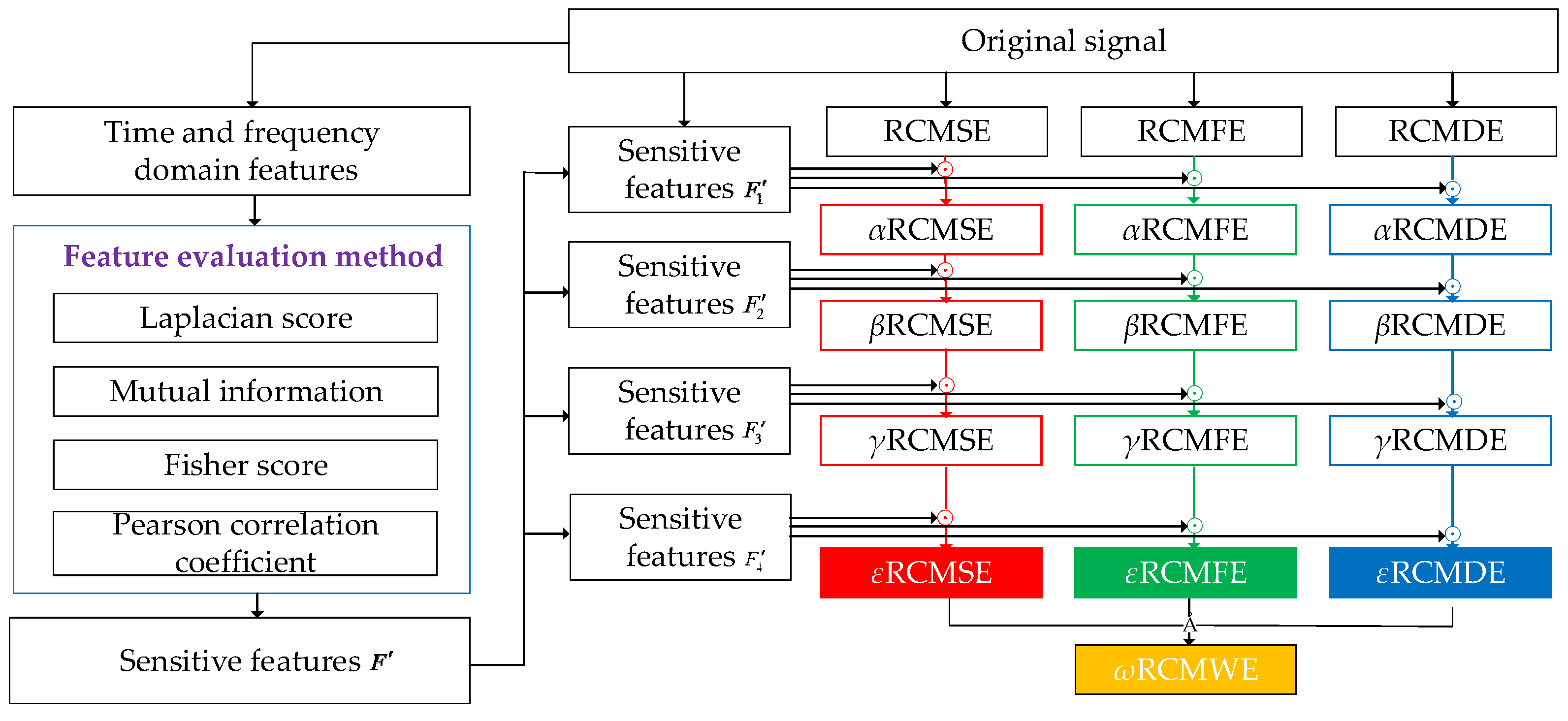
    where W uses the geometric mean, which can ignore the influence of outliers. It can indicate the average development of the data and present at the average trend of the overall data, which has less influence on the extreme values. The ω RCMWE calculation process is depicted in Figure 1.
Although the refined composite multi-scale entropy method provides an improvement over the traditional multi-scale entropy method, the distinction of fault categories still lacks stability. The time–frequency domain feature signals are selected by four types of feature evaluation methods, and the optimal sensitive features F i are used as the weighted values for the refined composite multi-scale entropy. The sensitive features F i = ( F 1 , F 2 , F 3 , F 4 ) , selected by the four types of feature evaluation methods, are used for Hadamard product operation with RCMSE, RCMFE and RCMDE in turn, thus obtaining α RCMSE, α RCMFE, α RCMDE, β RCMSE, β RCMFE, β RCMDE, γ RCMSE, γ RCMFE, γ RCMDE, ε RCMSE, ε RCMFE, and ε RCMDE. In particular, the sensitive features are weighted with RCMSE, RCMFE, and RCMDE for the first time to obtain α RCMSE, α RCMFE, and α RCMDE; then, they are weighted with α RCMSE, α RCMFE, and α RCMDE for the second time to obtain β RCMSE, β RCMFE, and β RCMDE; γ RCMSE, γ RCMFE, and γ RCMDE are obtained by weighting the sensitive features with β RCMSE, β RCMFE, and β RCMDE, respectively, for the third time; the sensitive features are weighted with γ RCMSE, γ RCMFE, and γ RCMDE for the fourth time to obtain ε RCMSE, ε RCMFE, and ε RCMDE, respectively; and, finally, the ω RCMWE is obtained using the weighting formula in Equation (23), with the multiple characteristic parameters and refined composite multi-scale entropy method. In the notation above, α, β, γ, and ε represent the first weighted value, the second weighted value, the third weighted value, and the fourth weighted value of the refined composite multi-scale entropy, respectively. The ω RCMWE method proposed in this paper can more accurately analyze the fault category and damage degree of rolling bearings in a qualitative manner. In order to evaluate the advantages and disadvantages of the weighted entropy method, experimental verification was conducted to prove the effectiveness of the proposed method.

4. Experimental Validation and Analysis of Results

4.1. Experimental Validation of Case Western Reserve University Dataset

4.1.1. Bearing Test Bench of CWRU

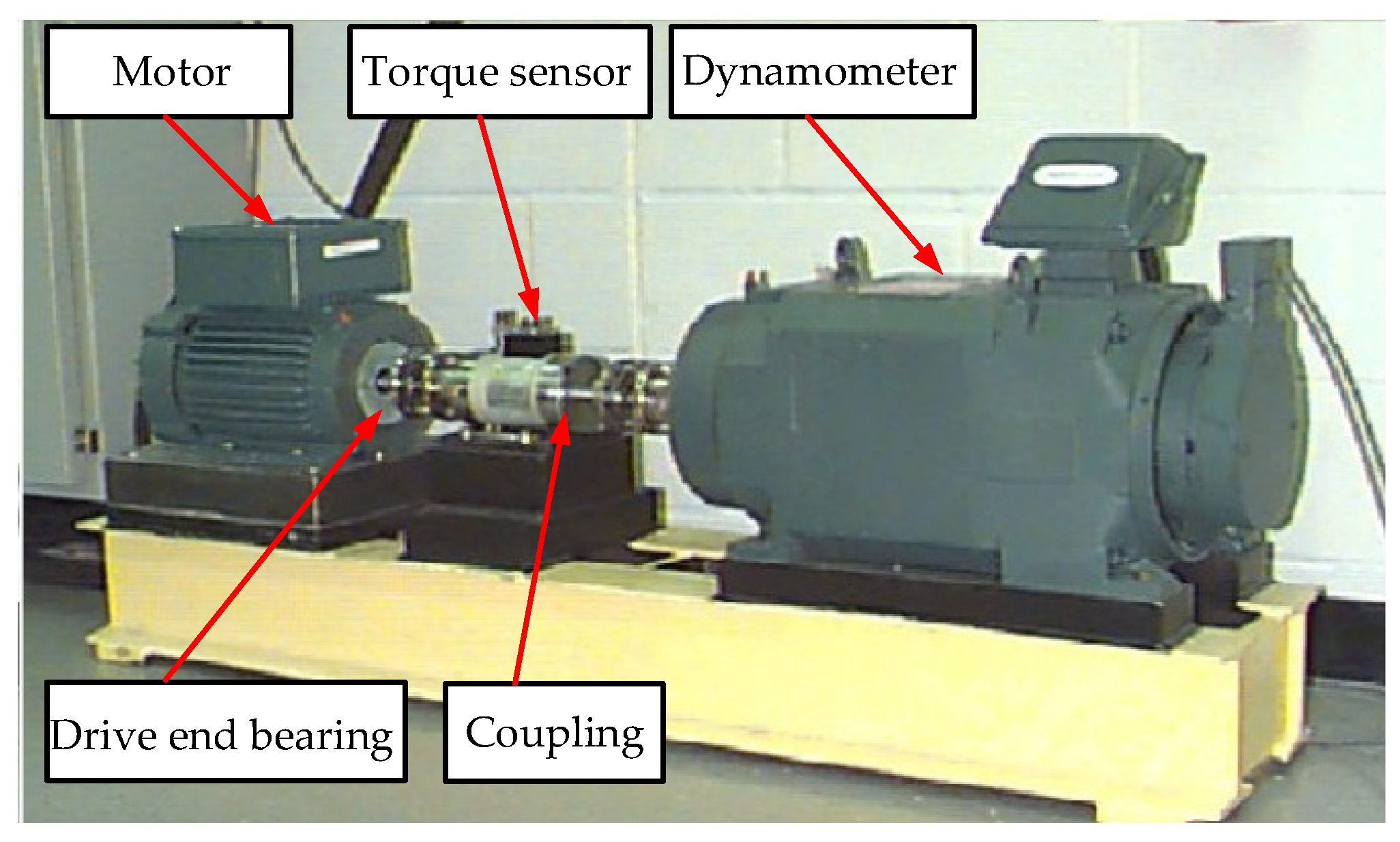
To verify the effectiveness of ω RCMWE for rolling bearing fault feature extraction, it was applied to experimental bearing data from Case Western Reserve University [45]. The bearing test bench of CWRU is shown in Figure 2, which consists of a three-phase asynchronous motor, a torsion sensor, an AC power measurement commutator, and a controller. The bearing under test supports the motor shaft and is placed at the input end of the motor (model 6205SKF-type deep groove ball bearing). EDM technology was used to set single-point faults on the bearing inner race, outer race, and ball, respectively. The fault was directly set to 0.007 inches, 0.014 inches, and 0.021 inches, in turn, and the speed was 1797 r/min.
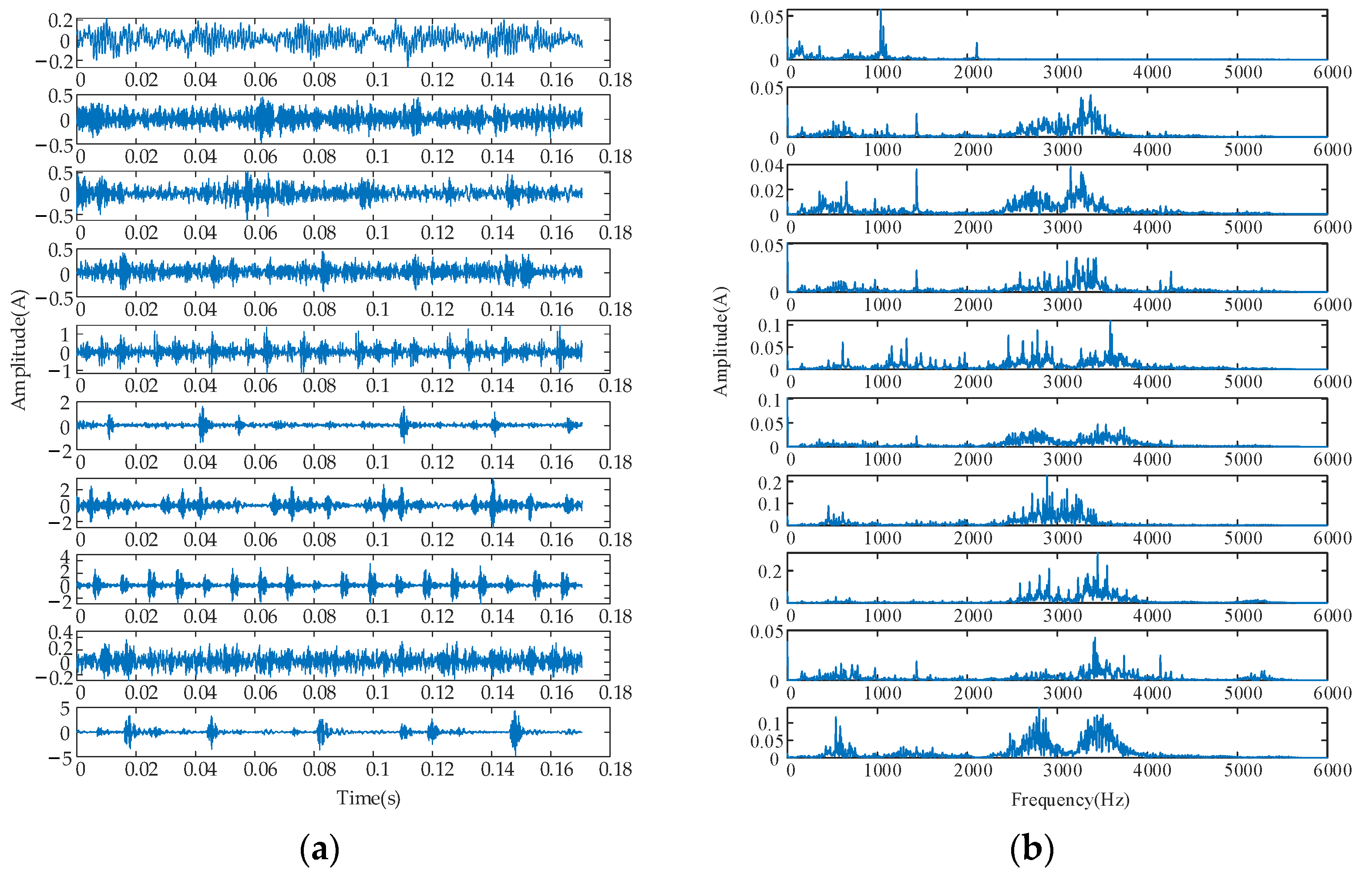
In the experiment, an acceleration sensor was used to obtain the vibration acceleration information for each state, and the experimental data were acquired at a sampling frequency of 12 KHz. A total of 50 groups were acquired for each fault state, where each group contained 2048 sample points. Four bearing states—healthy, inner race fault (IRF), outer race fault (ORF), and ball fault (BF)—and three fault damage dimensions under three fault states were considered in the experimental analysis. Ten types of fault time–frequency domain signals are shown in Figure 3, and specific fault state parameters are detailed in Table 2 and Table 3.
The time–frequency domain diagrams for the ten different fault types are shown in Figure 3. It can be seen, from the time-domain diagram, that when a fault occurred, the waveform and amplitude of the vibration signal changed, to some extent. The amplitude of the outer race vibration signal was the largest, followed by the inner race, while that of the ball was the smallest. The vibration signals of the fault state presented periodic impacts, especially the outer race; however, it was impossible to distinguish the fault types accurately according to the time–frequency domain.
Feature evaluation mainly measures the corresponding relationship between features and categories. By evaluating the score results, the ranking of features (from largest to smallest) was obtained, and the sensitive features were determined. Based on the experimental data from CWRU initial feature set LS, PS, FS, and MI method ranking, the obtained fault feature importance ranking is provided in Table 4.
The feature evaluation method also allowed us to determine the frequency domain indicators more related to the bearing failure state. The feature ranking results are given in Table 5. In the LS-based feature ranking, the frequency-domain feature x 15 had higher importance. In the PS-based feature ranking, x 3 in the time-domain features was important. In the FS-based feature ranking, the time-domain feature x 5 was very important. Finally, in the MI-based feature ranking, the frequency-domain feature x 15 had high importance. It can be seen that time-domain features had a certain position in measuring the importance of features, but the overall importance of time-domain features was low. This indicates that the time domain features are not as crucial for the extraction of sensitive features in the bearing vibration signal processing. Instead, it is important to fuse the time–frequency domain features to extract the features with high importance and sensitivity, in order to further improve the bearing state identification performance.

4.1.2. Entropy Feature Analysis of Rolling Bearings under Different Damage Degrees

The entropy value features were obtained under the bearing failure states No. 1–No. 10 using the Hadamard product, in order to obtain α RCMSE, α RCMFE, α RCMDE, β RCMSE, β RCMFE, β RCMDE, γ RCMSE, γ RCMFE, and γ RCMDE. Then, the entropy indices were weighted and combined to obtain ω RCMWE. The performance of the entropy method in distinguishing between healthy and fault states was evaluated.
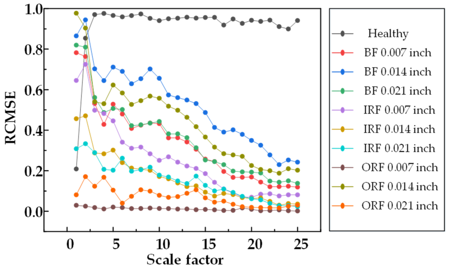
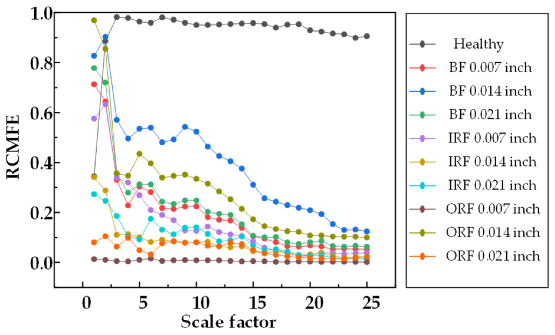
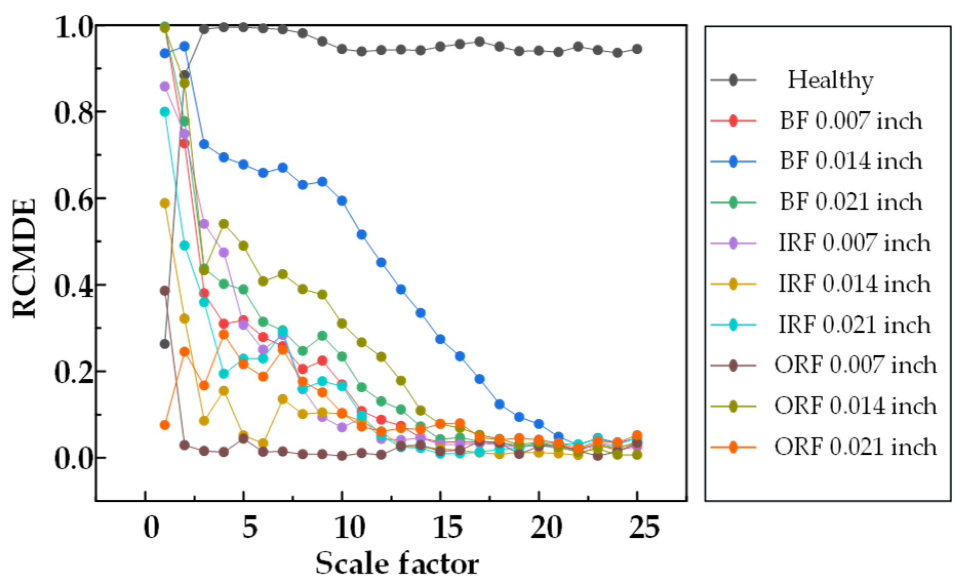
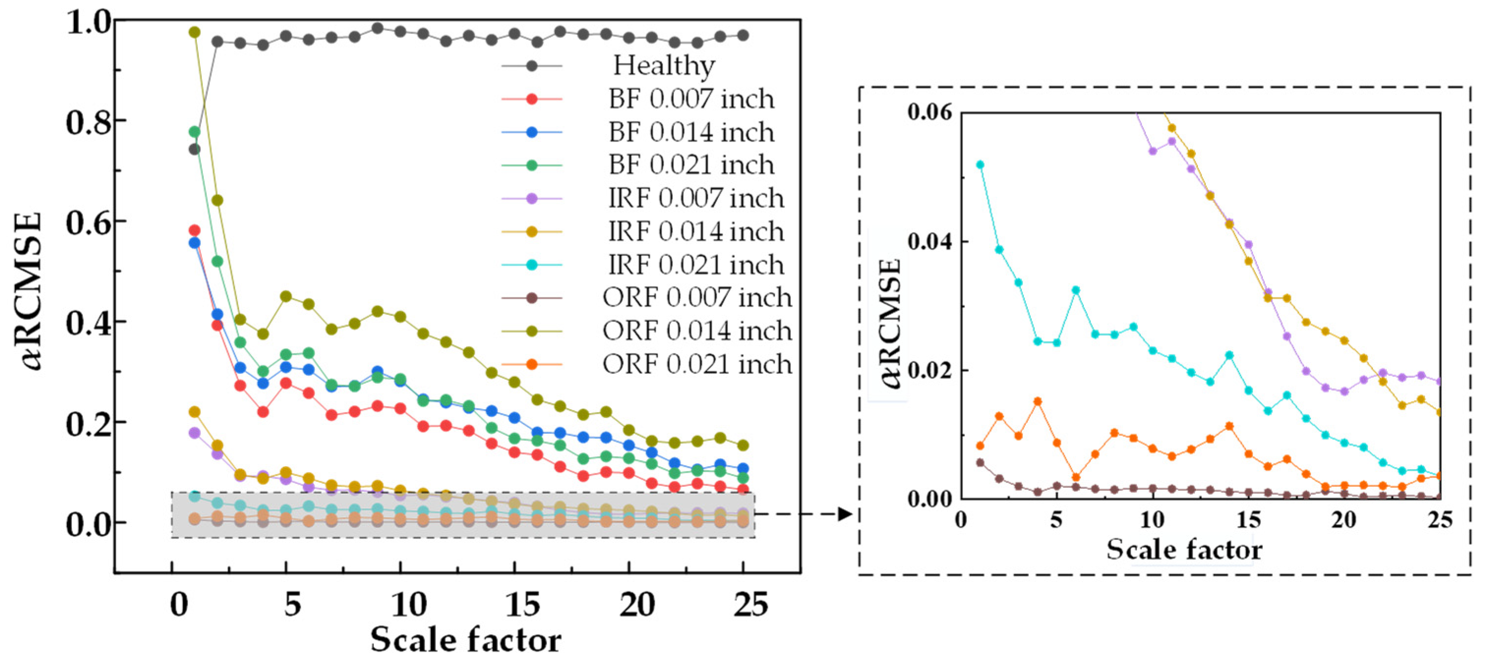
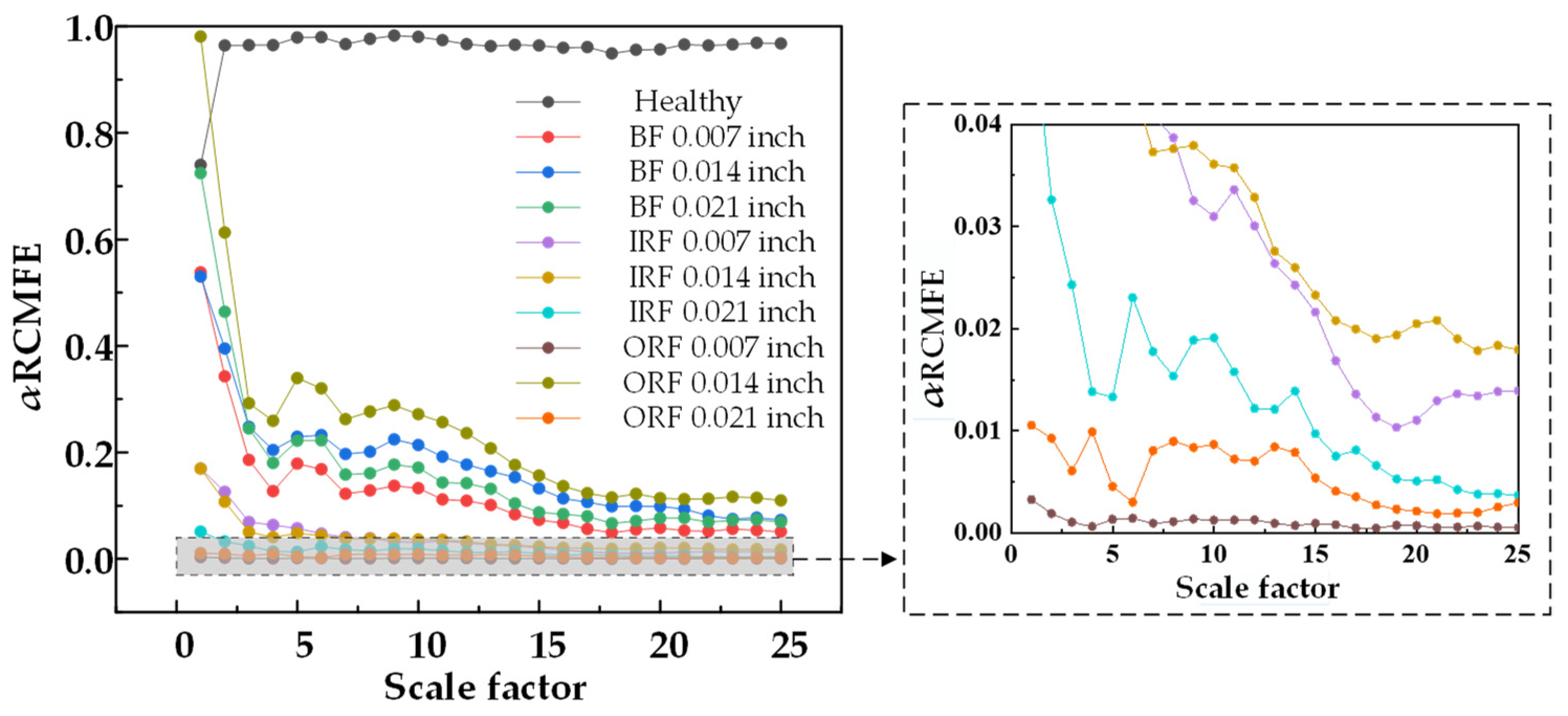
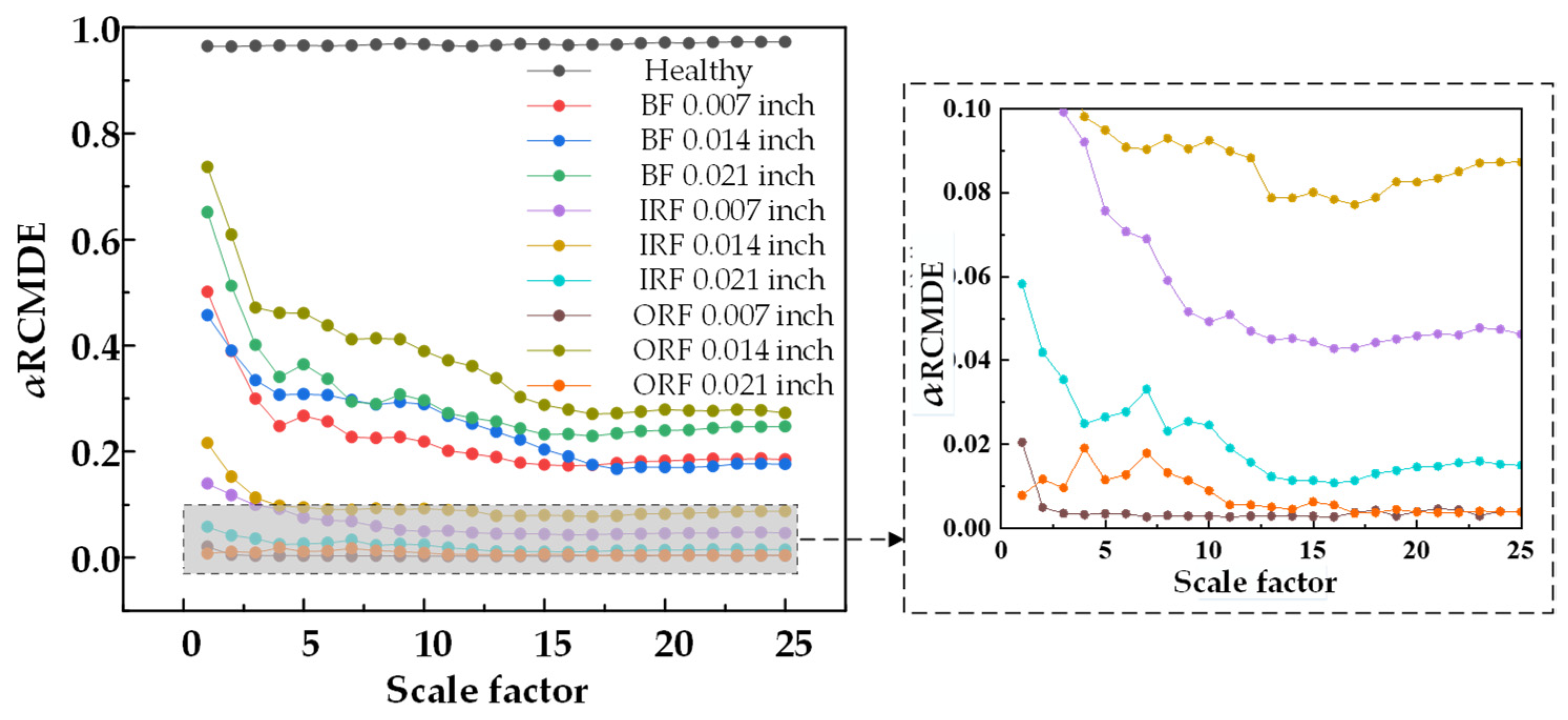
Figure 4, Figure 5 and Figure 6 show that the entropy values of RCMSE, RCMFE, and RCMDE are seriously aliased in the first three scales. Although normal and abnormal states can be distinguished in the whole scale, the entropy values of different faults are aliased and local stability cannot be maintained. Figure 7, Figure 8 and Figure 9 show that, for α RCMSE and α RCMFE weighted by single feature parameters, under the first five scale factors, the normal entropy value and other faults overlap each other, and the normal and abnormal fault interval ranges could not be distinguished. However, with an increase in the scale factor, the difference between normal entropy and abnormal entropy became obvious. Although α RCMDE could distinguish normal and abnormal fault intervals in the whole scale factor, it presented the problem of overlapping between different faults. When the rolling bearing works in a healthy state, the vibration is random. Once the rolling bearing fails, the fault part becomes a driving source, constantly producing regular and periodic impacts. Therefore, the obtained vibration signals have obvious regularity and increased self-similarity, leading to decreases in complexity and entropy. In addition, under most scaling factors, the entropy of the ball fault signal was higher than that of the inner and outer race faults. This was mainly because, when a fault occurs, the vibration signal of the system has obvious impact characteristics, while different fault locations have different impact frequencies. Therefore, the faults at different locations lead to different complexity in the resulting vibration signals. As the outer race rolling bearing is fixed on the bearing seat, when the outer race faults, the impact characteristic frequency of the vibration signal is singular and simple. In addition, compared with the inner race and ball faults, the outer race fault had the smallest characteristic frequency, so its self-similarity and regularity were also the most obvious, which led to the fastest decline in the entropy curve of the vibration signal with its increase. As the inner race rotates with the rotating shaft, the fault characteristic frequency of the ball is greater than that of the inner race. Therefore, the fault of the rolling vibration signal ball is more complex than that of the inner race and the outer race, in theory. The entropy value at a single scale cannot effectively distinguish the fault category. When the scaling factor is equal to 1, the multi-scale entropy of the original vibration signal will be reduced to the sample entropy. As the entropy value of the normal rolling bearing vibration signal is lower than that of the rolling bearing fault vibration signal, it is easy to draw the wrong conclusion that the fault vibration signal of rolling bearing is much more complex than that of an ordinary rolling bearing. Therefore, compared with the traditional entropy analysis based on a single scale, the multi-scale entropy method can better reflect the fault state.
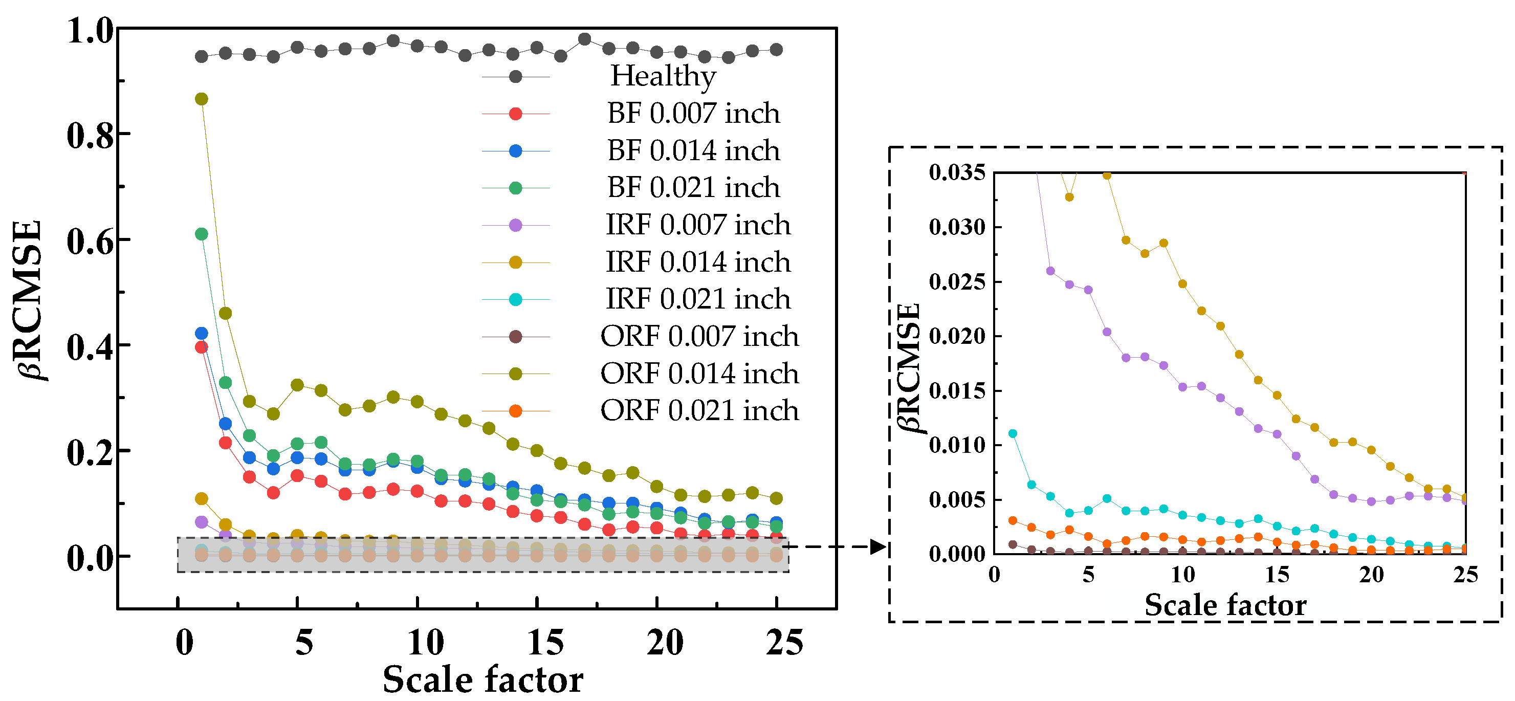
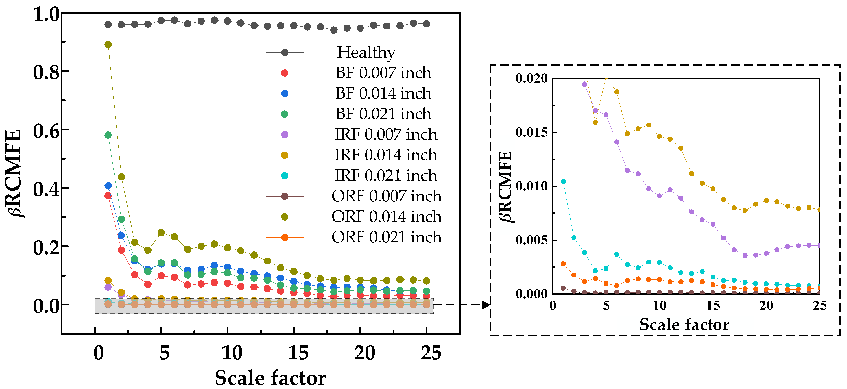
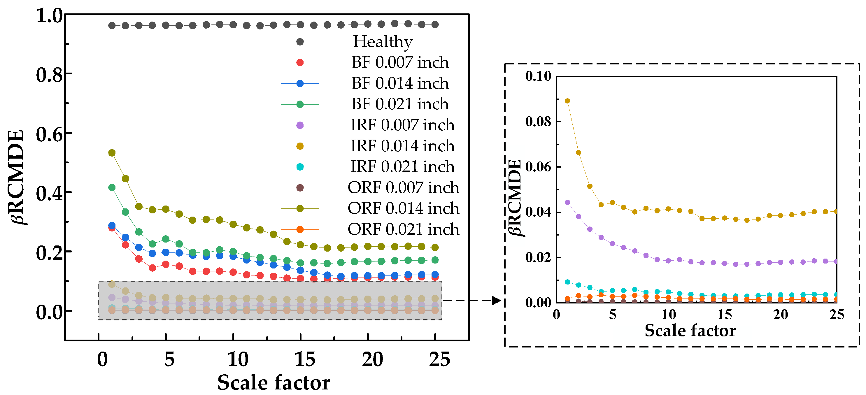
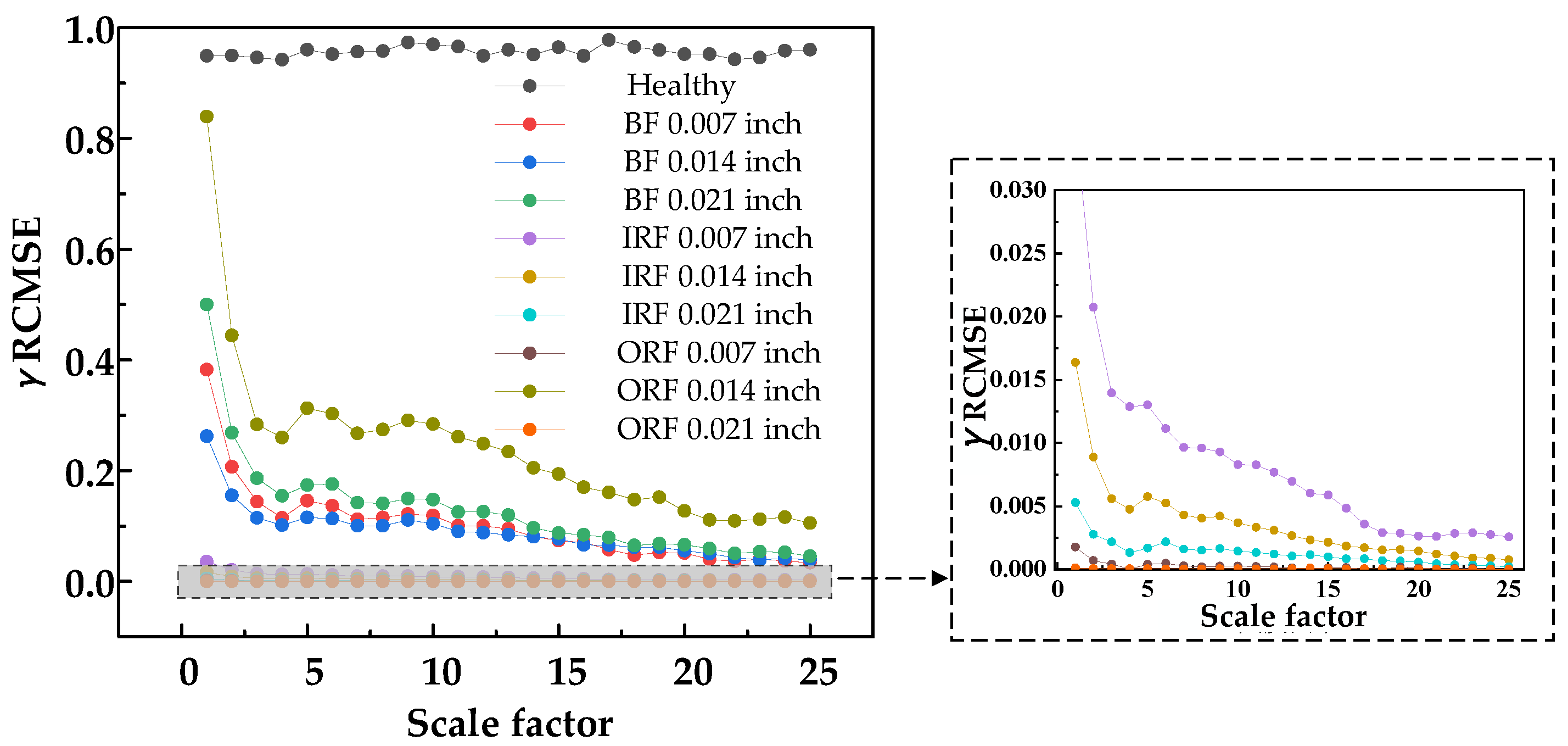
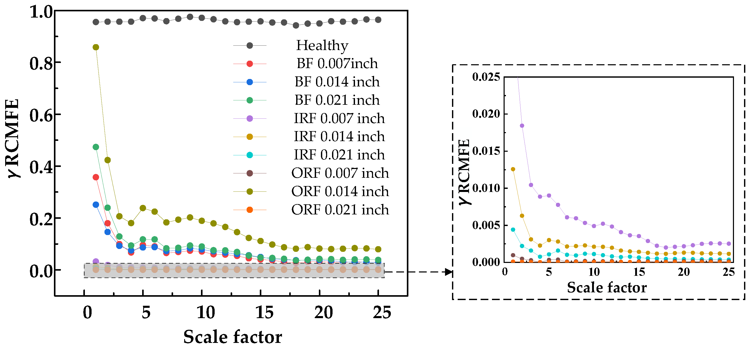
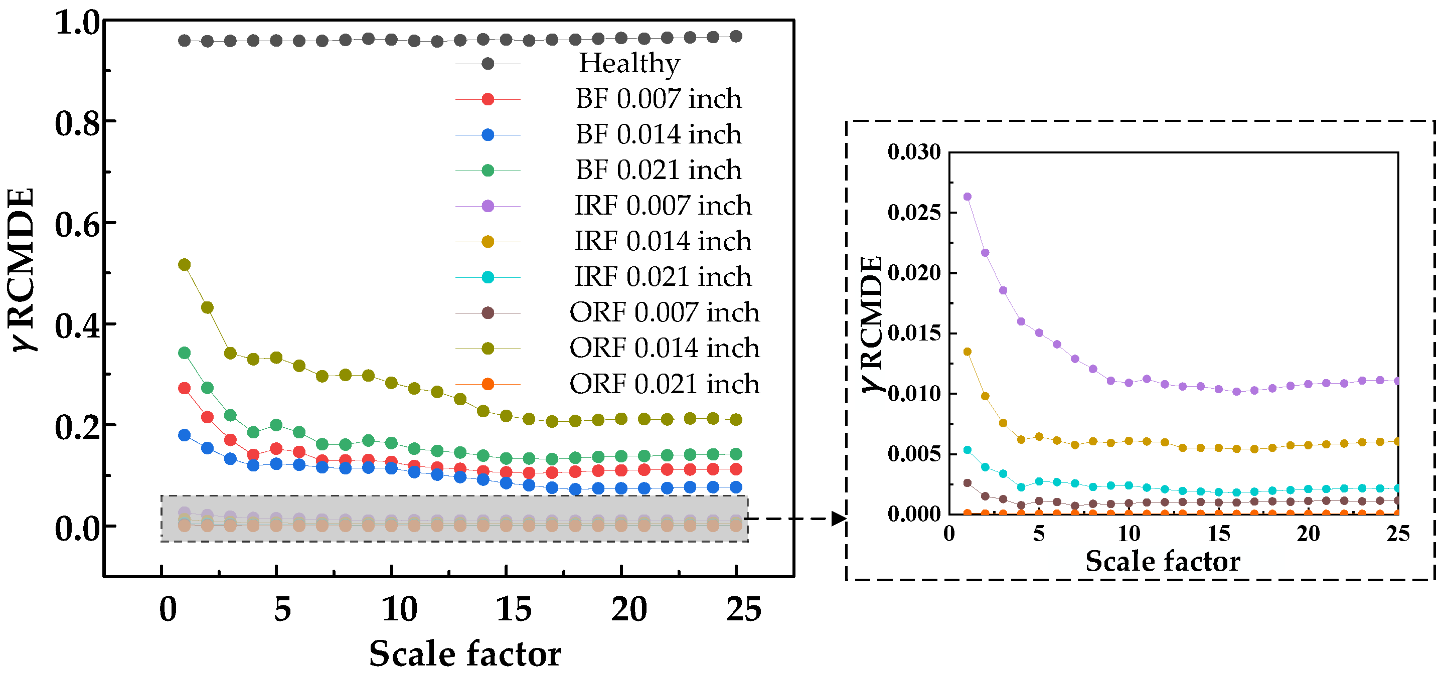
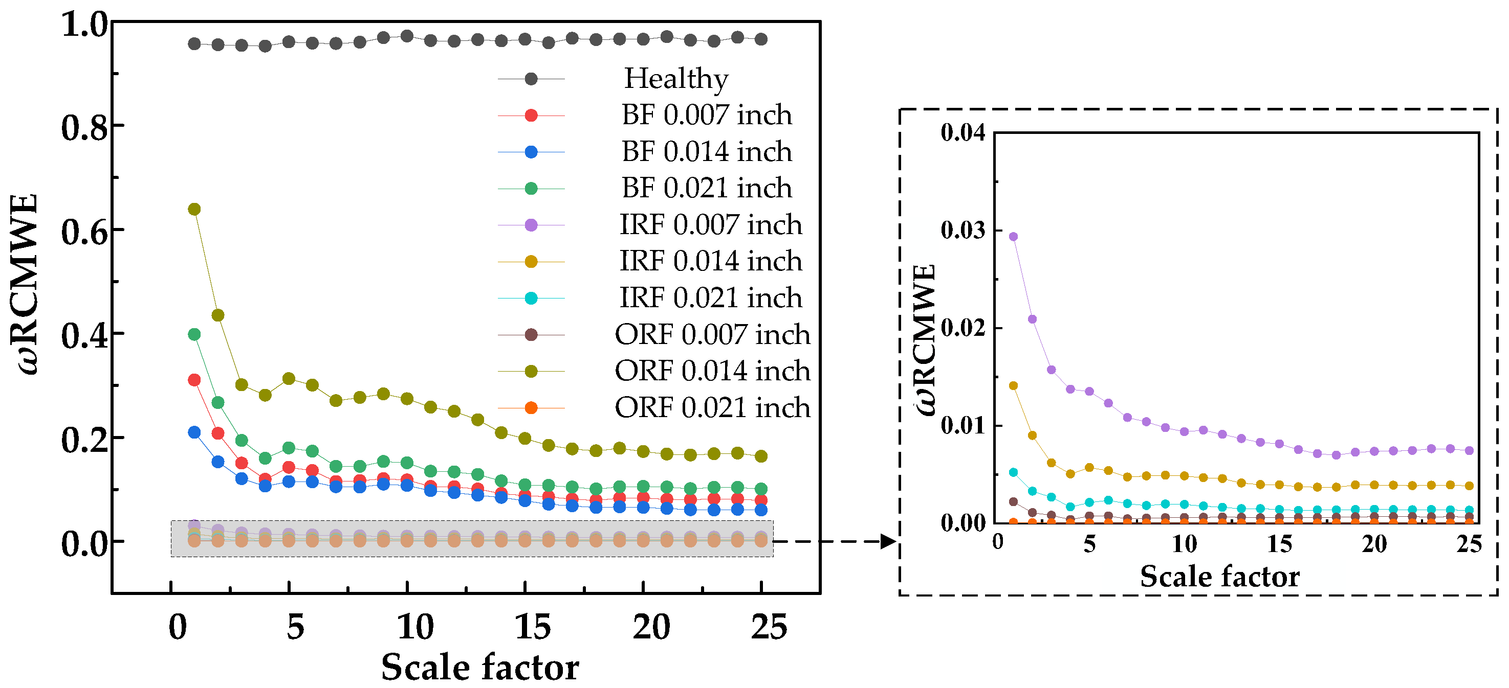
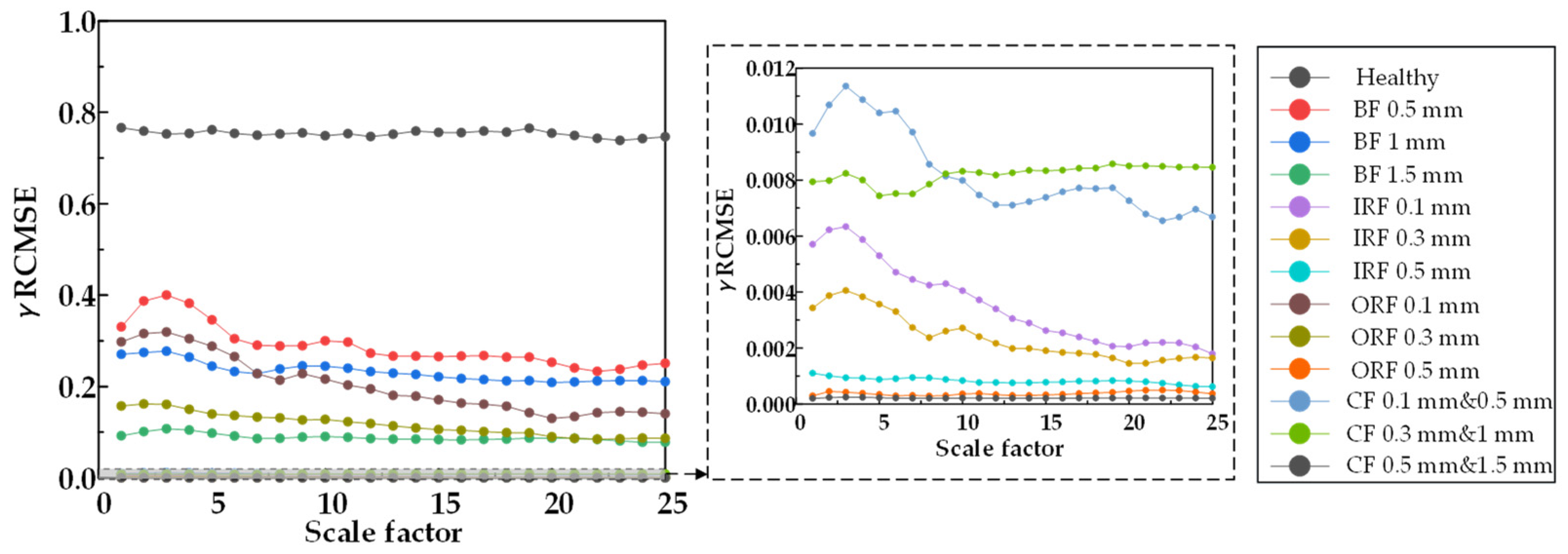
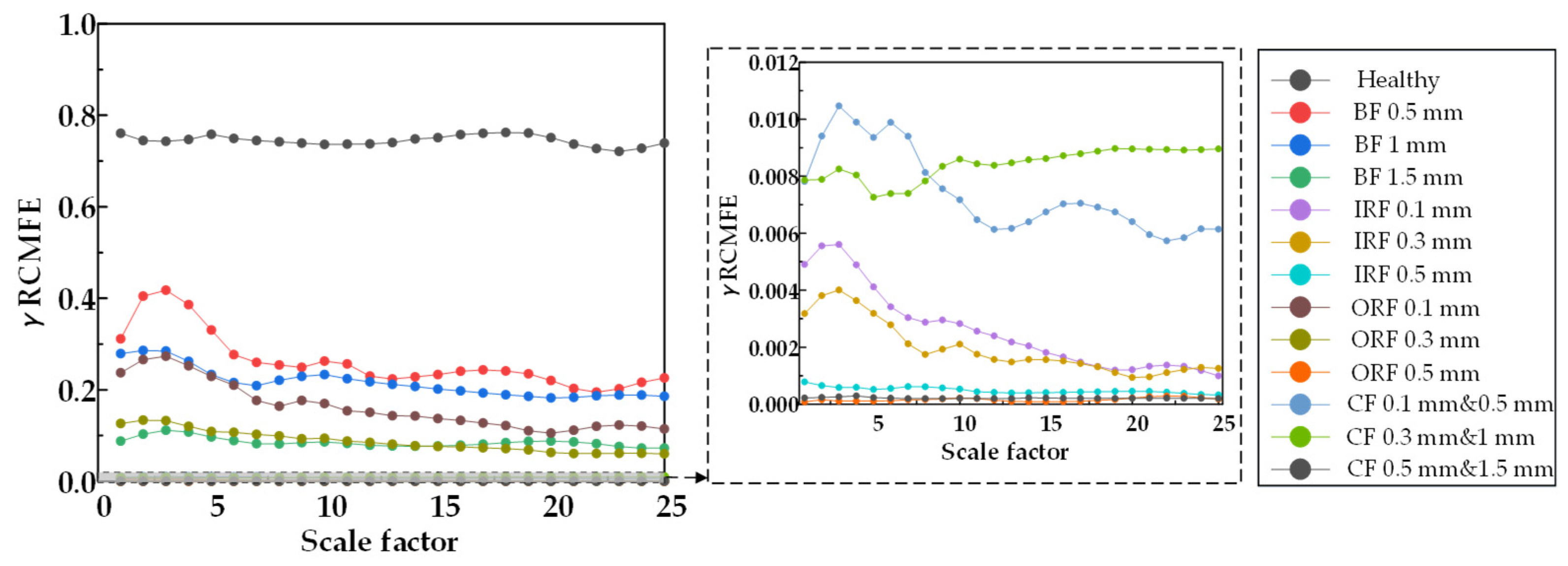
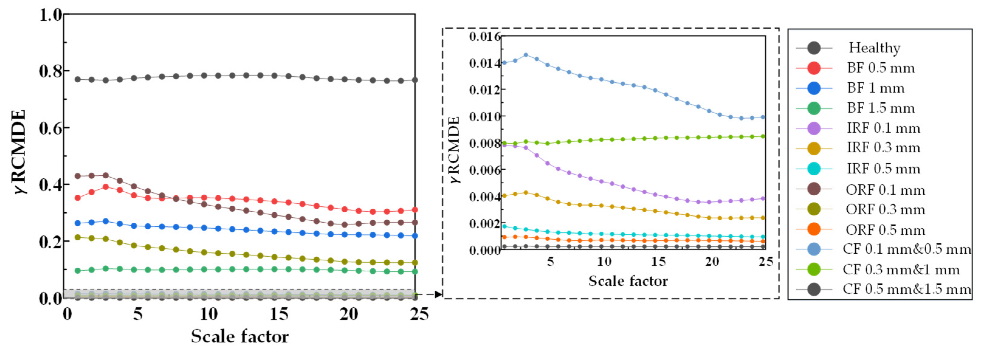
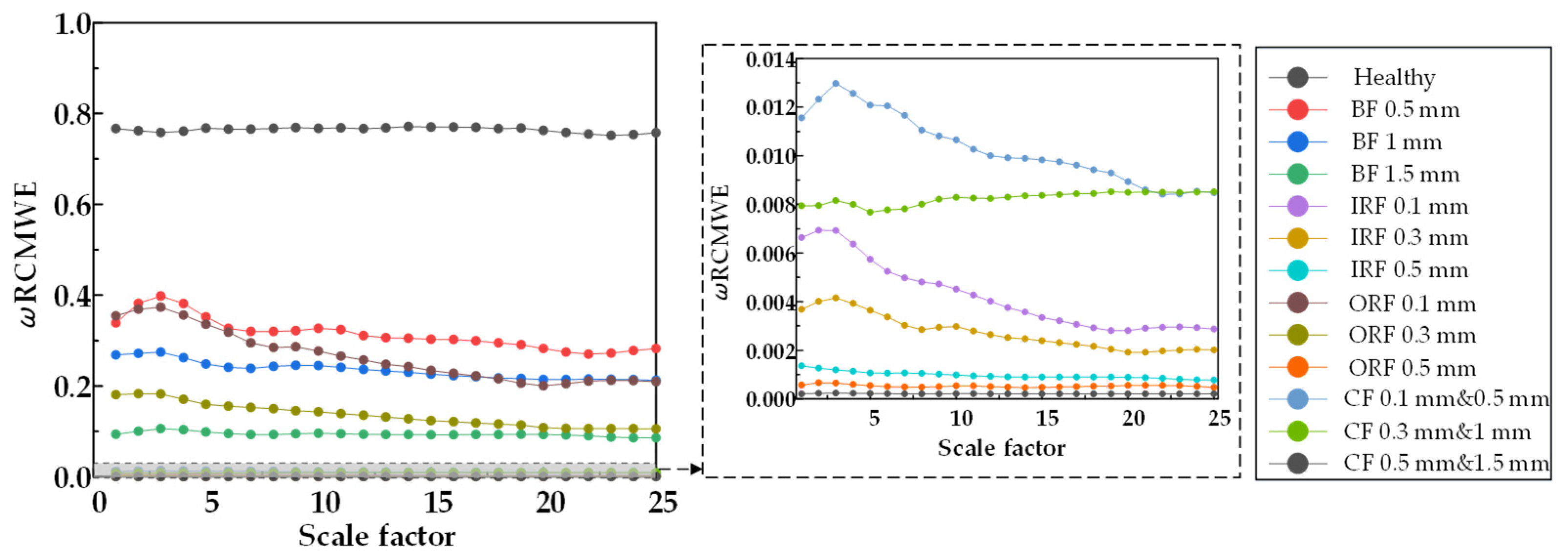
Figure 10, Figure 11 and Figure 12 show that β RCMSE, β RCMFE, and β RCMDE, weighted by double characteristic parameters, could not coincide with the entropy values of other faults on the whole scale factor. With an increase in scale factor, the normal and abnormal entropy values could be clearly distinguished. Compared with the entropy values weighted by single feature parameter, the entropy values weighted by double feature parameters of β RCMSE, β RCMFE, and β RCMDE presented a more obvious distinction between normal and abnormal entropy, which can maintain stability in multi-scale state, but there is still the problem of over-lapping between different faults. It can be seen, from Figure 13, Figure 14, Figure 15 and Figure 16, that γ RCMSE, γ RCMFE, γ RCMDE and ω RCMWE weighted by multi-feature parameters also could not coincide with the entropy values of other faults on the whole scale factor. With an increase in scale factor, the normal and abnormal entropy values could be clearly distinguished. Compared with the entropy values weighted by single and double feature parameters, the difference between normal and abnormal entropy values was more obvious in the multi-feature parameter weighted γ RCMSE, γ RCMFE, γ RCMDE, and ω RCMWE entropy value methods. Therefore, γ RCMSE, γ RCMFE, γ RCMDE, and ω RCMWE can force the different entropy values in the overlapping relationship as far apart as possible, while maintaining their stability in the multi-scale state. In particular, γ RCMDE and ω RCMWE could clearly and correctly identify different fault types and fault damage conditions, and the entropy value between different fault types did not overlap on the whole scale. The entropy values of γ RCMDE and ω RCMWE after multi-feature weighting reached a stable value from the initial scale, and the scale itself extended to all scales. Therefore, γ RCMDE and ω RCMWE can be used as baseline entropy indicator values for health fault detection.
Overall, the weighted entropy method significantly improved the health fault detection performance. The weighted entropy of the health state was greater than the entropy of the fault state. This was due to the weighting parameter, which could control any change in the entropy of the healthy signal at all scales. Notably, γ RCMDE and ω RCMWE were superior to γ RCMSE and γ RCMFE as baseline indicators. It was found that, from the initial scale, the fault entropy value presented a sharp downward trend and, so, the degradation laws for different faults of bearings were satisfied. With an increase in the scale factor, the entropy value changed in an exponential decay form. Therefore, γ RCMDE and ω RCMWE can serve as effective indicators of bearing deterioration. In summary, the above analysis showed that γ RCMDE and ω RCMWE are very suitable for rolling bearing fault detection and diagnosis, and may be used as effective tools for mechanical fault diagnosis and condition monitoring.
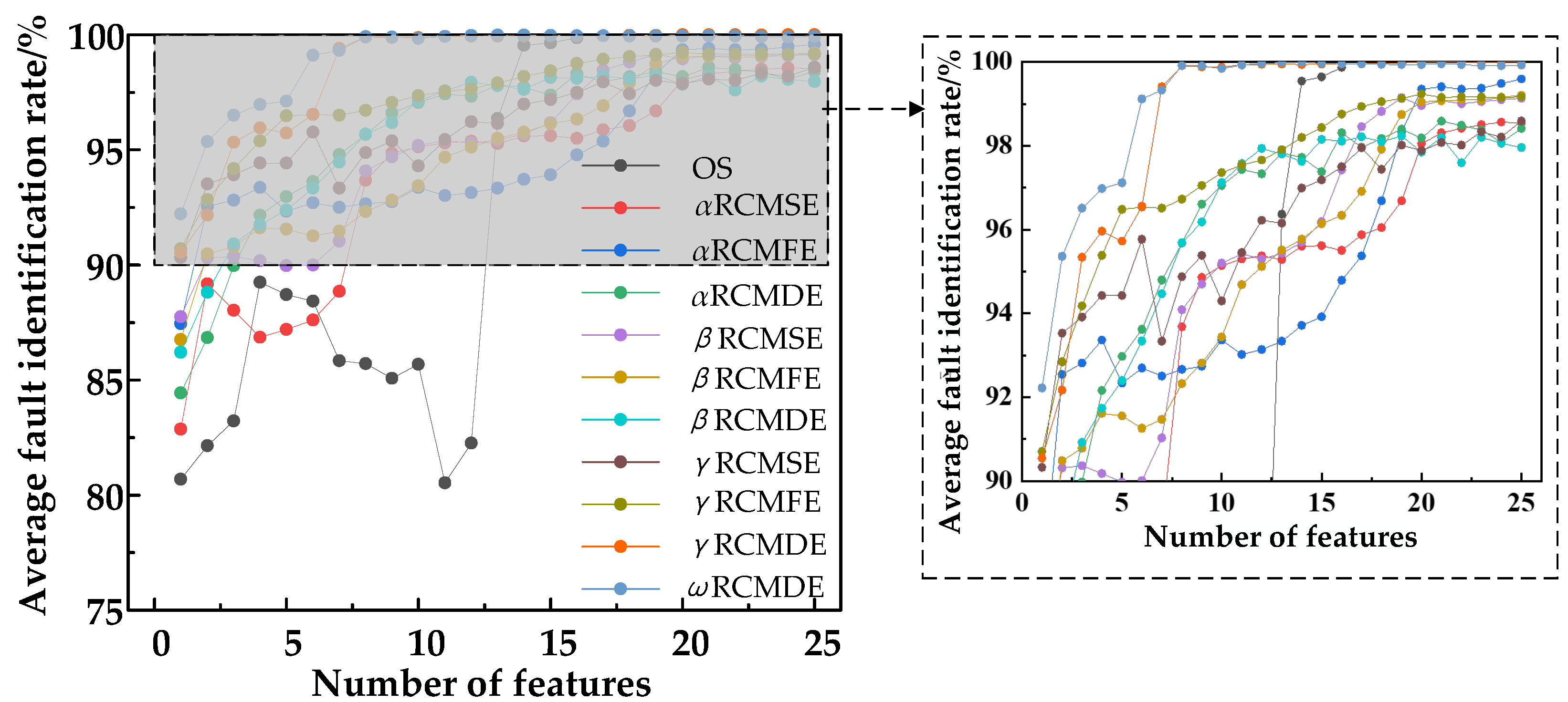
To further quantify the feature extraction effect of the weighted entropy method, for the 11 feature sets of the OS, α RCMSE, α RCMDE, α RCMFE, β RCMSE, β RCMDE, β RCMFE, γ RCMSE, γ RCMDE, γ RCMFE, ω RCMWE, we, respectively extracted 1 to 25 features from the initial features and input them to the classifier as training and testing samples, in order to achieve fault classification and recognition. A total of 10 groups of samples under 10 working conditions were randomly selected for training, and the remaining 40 groups of samples were tested. There were 100 training samples and 400 test samples under the 10 working conditions of the rolling bearings. For the classifier, we used the LIBSVM toolbox, where the SVM kernel function was the radial basis function [46]. The penalty factor was set to 10, the kernel function parameter was set to 20, and the cycle test was performed 50 times. The training samples and training tags were input into the multi-class classifier based on SVM for training, and a model containing fault feature information was obtained after training. The classifier used this model to analyze the test samples and realized fault diagnosis by comparing the output results of the classifier with the actual results. The bearing fault recognition results obtained from the 11 feature extraction methods are shown in Figure 17.
From Figure 17, we can see that the original time–frequency domain feature OS initially decreased with an increase in the number of features, then increased along with the number of features. The α RCMSE, α RCMFE, α RCMDE, β RCMSE, β RCMFE, and β RCMDE fault accuracy increased with an increase in the scale factor, and the overall fault identification rate could be guaranteed to be above 72%. With γ RCMSE, γ RCMFE, and γ RCMDE, the fault accuracy increased with an increase in scale factor, and the overall fault identification rate could be guaranteed to be above 98%. The results for ω RCMWE and γ RCMDE were better than those for the other methods. From the first eigenvalue, based on the use of ω RCMWE and γ RCMDE, the fault identification rate reached 100%. These results indicate that the weighted entropy method with multiple characteristic parameters can identify the fault types of bearings under different damage conditions at any scale. In particular, the use of the weighted RCMWE and γ RCMDE for fault identification provided more stable results than the other methods. For α RCMSE, α RCMFE, α RCMDE, β RCMSE, β RCMFE, and β RCMDE, the failure recognition rate for the first few scale factors was decreased, mainly due to the influence of the weighted index increasing the difference between normal and abnormal entropy, thus magnifying the influence of entropy. The above analysis indicated that the γ RCMDE and ω RCMWE method based on multi-feature parameter weighting proposed in this paper was superior to the other methods for fault diagnosis in the bearing experimental data.

4.2. Experimental Verification of Bearing Fault Diagnosis Data Set

4.2.1. Test Bench of Bearing Fault Diagnosis

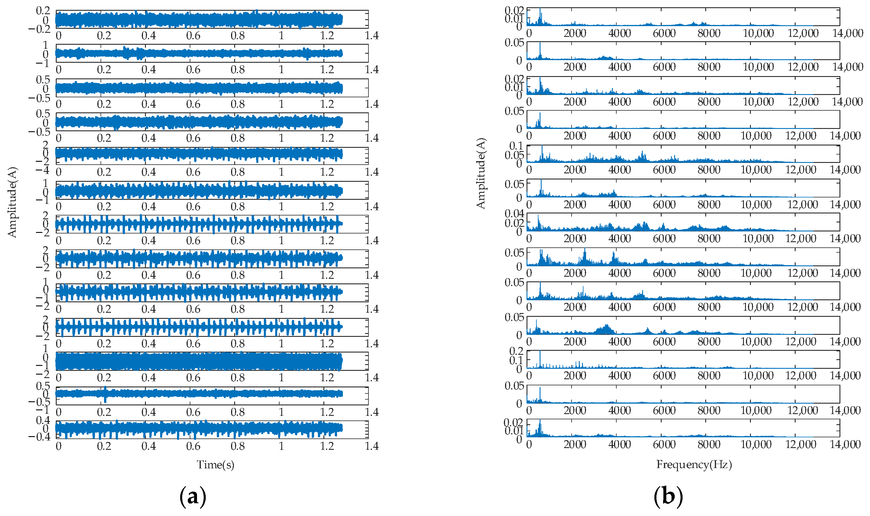
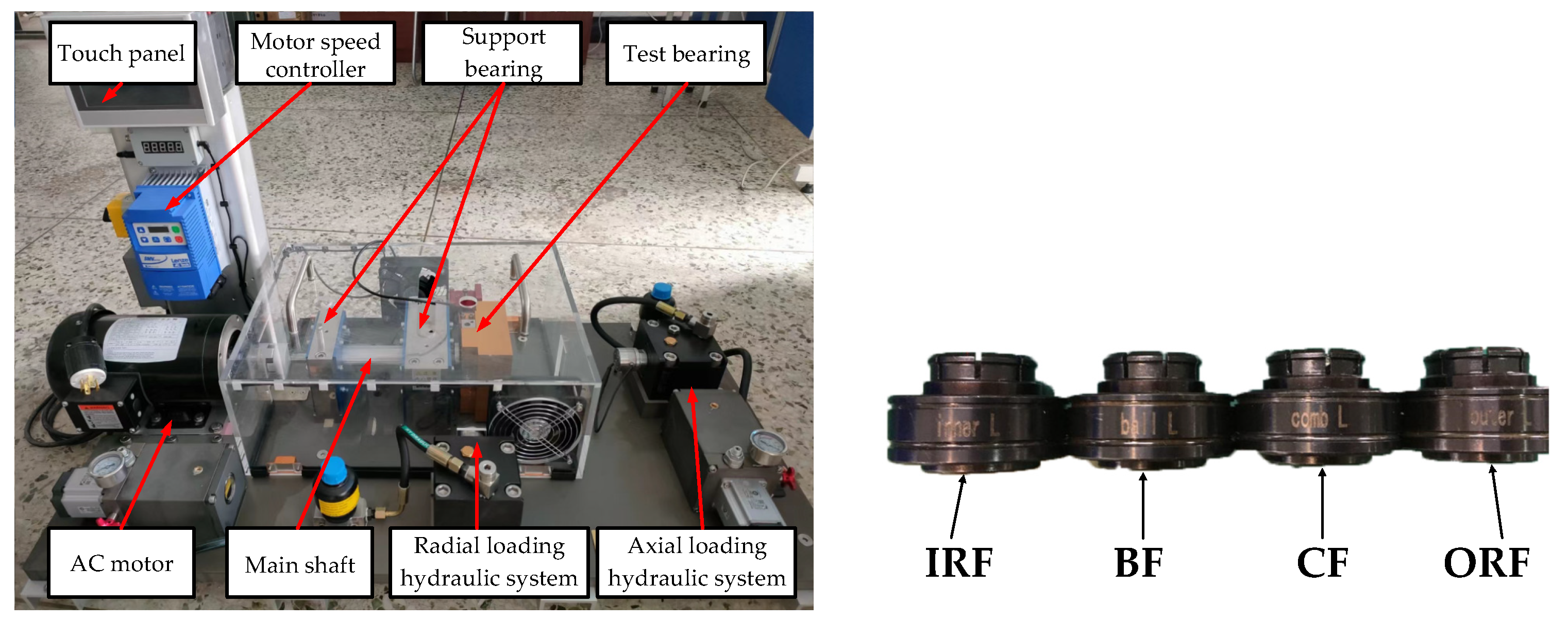
The bearing fault diagnosis test bench consisted of a touch panel, motor speed controller, motor, radial loading hydraulic system, axial loading hydraulic system, main shaft, two support 6210 bearing, and 18,720 bearing, the ER-16K bearing to be measured, force arm beam adjusting device, and hydraulic device for dismantling bearings, as shown in Figure 18. The acceleration sensor obtained the vibration acceleration information of 13 bearing fault states, including 10 single-point faults and 3 compound faults (CF). The experimental data were obtained at a sampling frequency of 25.6 KHz. A total of 10 groups were collected under each fault state, where each group included 32,768 sample points. Taking the working condition of bearing speed of 2400 r/min and bearing a radial load of 200 kg as an example, fault feature extraction analysis was carried out, considering different fault positions and fault dimensions. The time–frequency domain signals of the 13 types of faults are shown in Figure 19, and the specific parameters of different fault states are given in Table 6 and Table 7.
To verify the validity of ω RCMWE as the index for judgment of the abnormal state of bearings, the damage data of 13 types of bearings in different fault states were used for verification. First, the obtained original vibration signal was normalized. Then, 15 characteristic indices of time–frequency domain characteristics were obtained. The constructed time–frequency domain feature set was sorted using the LS, PS, FS, and MI methods. The ranking of fault feature importance is provided in Table 8.
Through the feature evaluation method, we also found that the frequency domain index was more related to the bearing fault state, as shown in Table 9. In the feature ranking based on LS, the smaller the score, the higher the importance. It can be seen that the frequency-domain feature x 15 was more important. In the feature ranking based on PS, the higher the score, the higher the importance, and the frequency-domain feature x 14 was more important. In feature ranking based on FS, the higher the score, the more important the feature. The time-domain characteristic x 1 was found to be important. In the MI feature ranking, the higher the score, the higher the importance. It can be seen that the frequency-domain feature x 14 was important.

4.2.2. Entropy Characteristic Analysis of Rolling Bearings under Compound Fault Diagnosis

We replaced No. 1–No 13. And carried out weighted entropy analysis, in order to obtain α RCMSE, α RCMFE, α RCMDE, β RCMSE, β RCMFE, β RCMDE, γ RCMSE, γ RCMFE, γ RCMDE, and ω RCMWE. Then, the performance of the entropy method in distinguishing the healthy and compound fault states of the rolling bearing was evaluated.
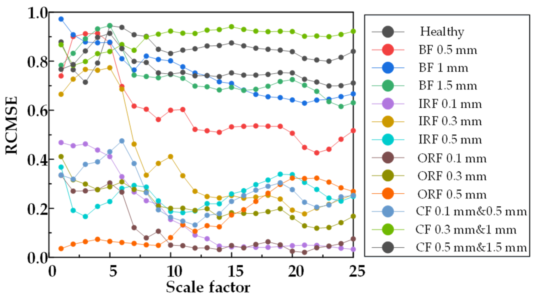
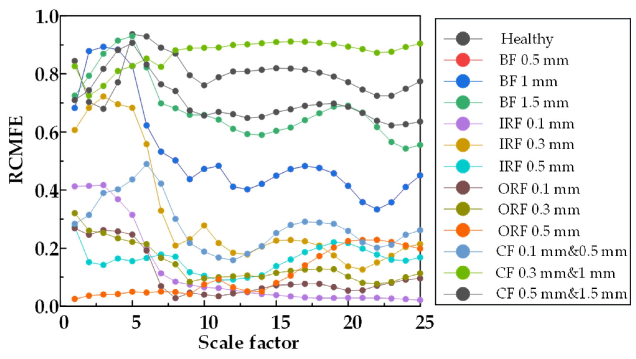
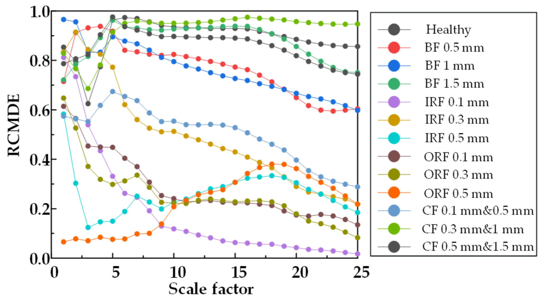
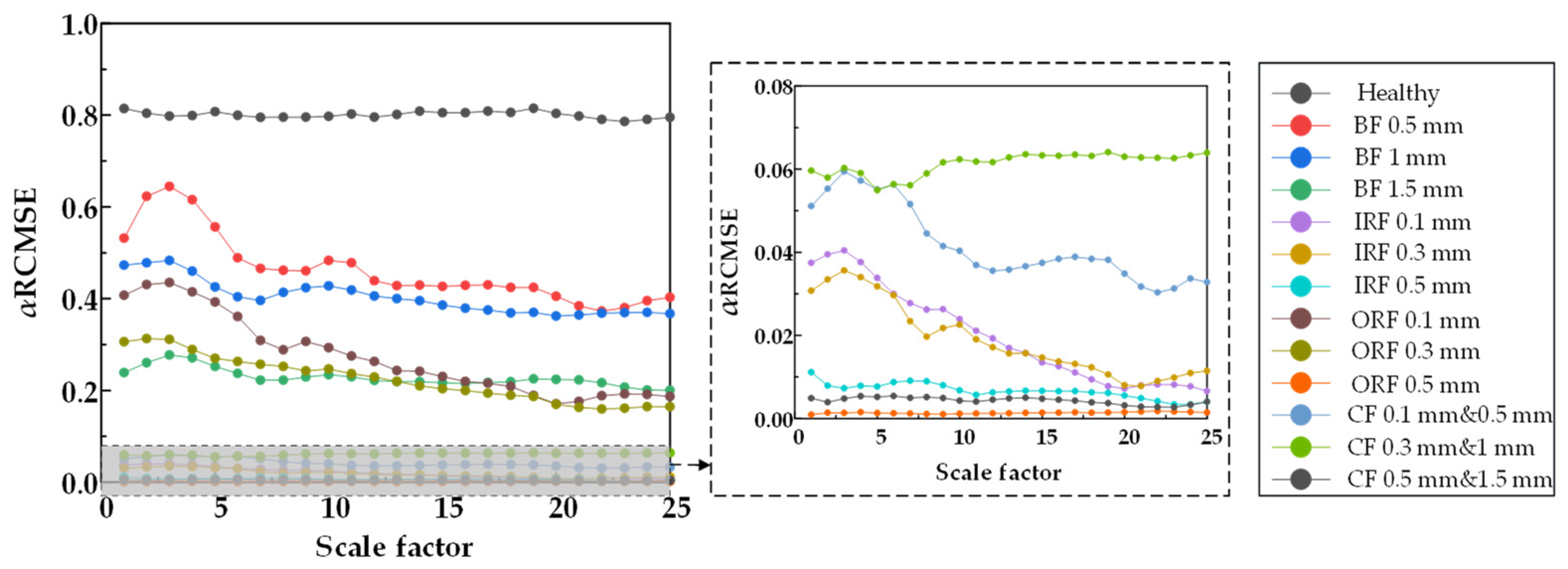
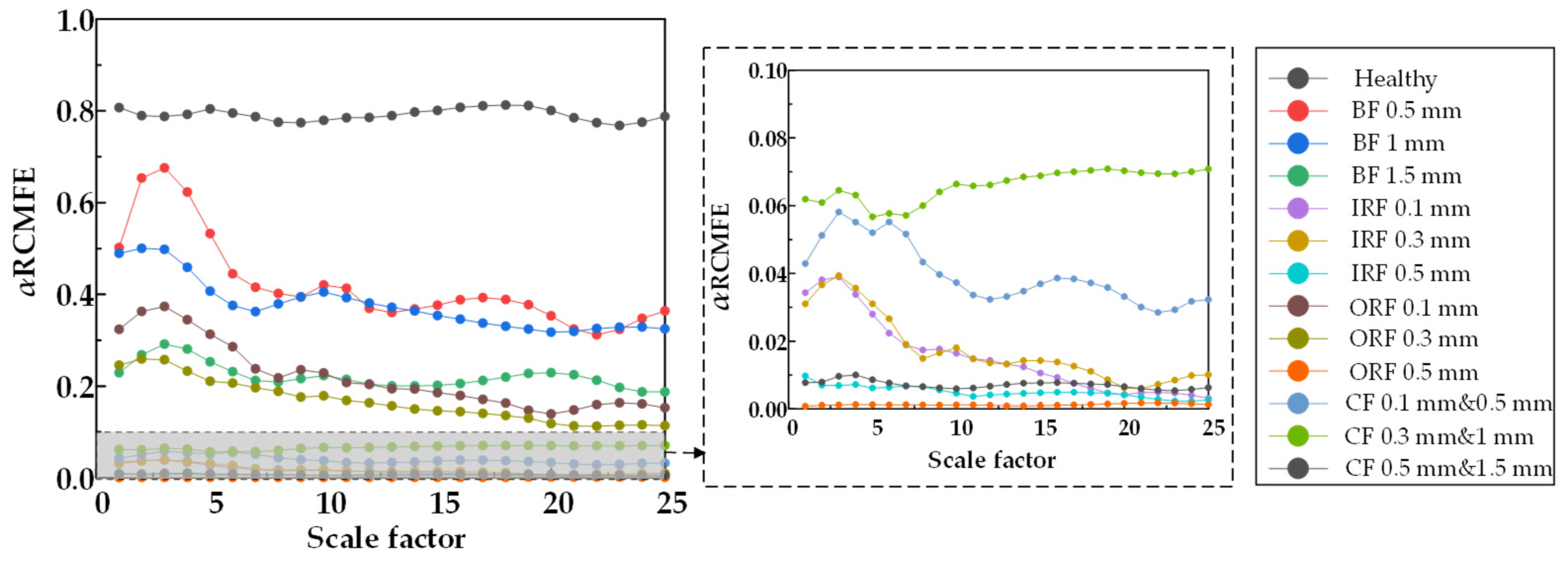
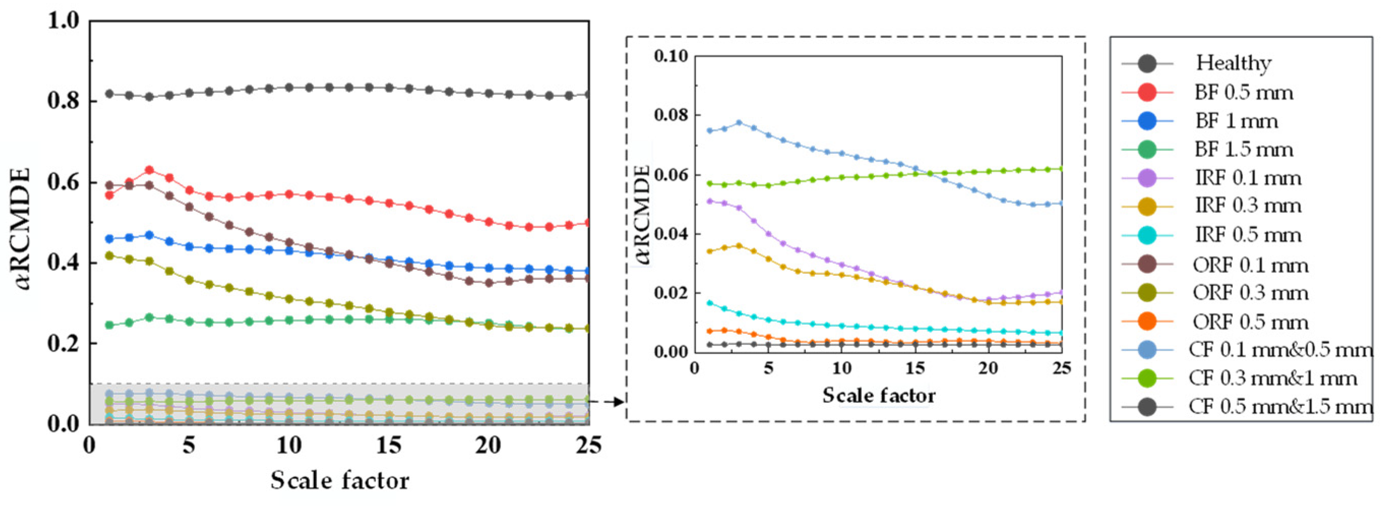
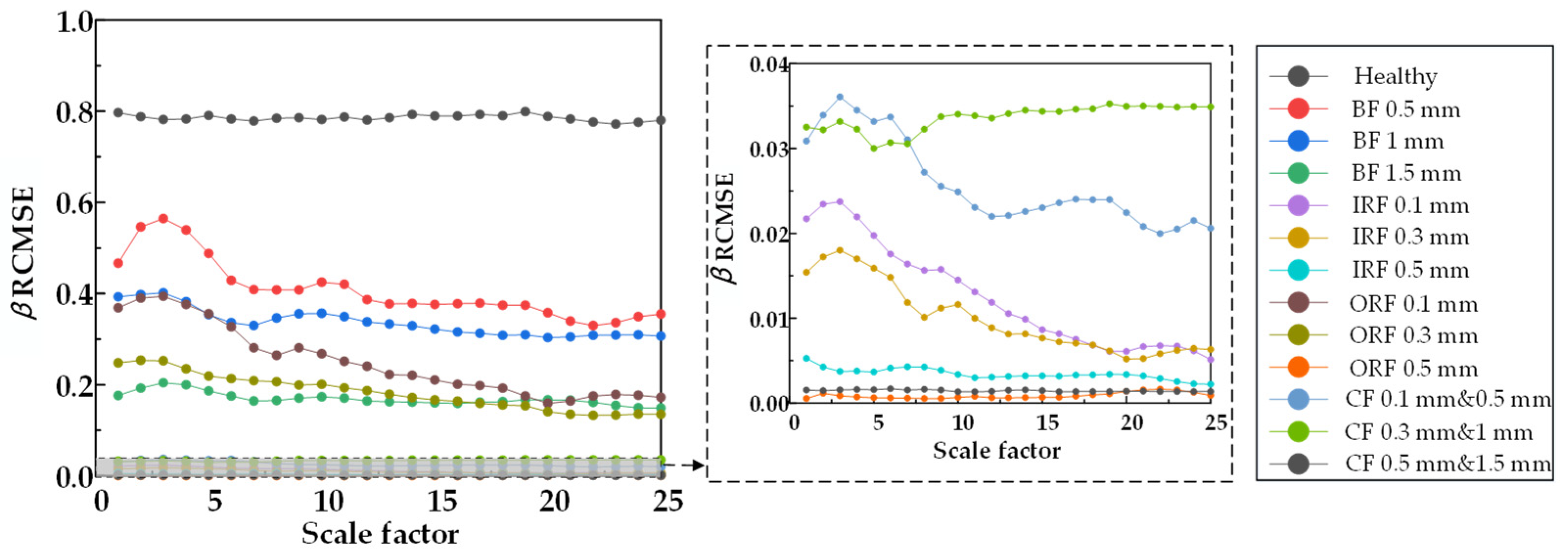
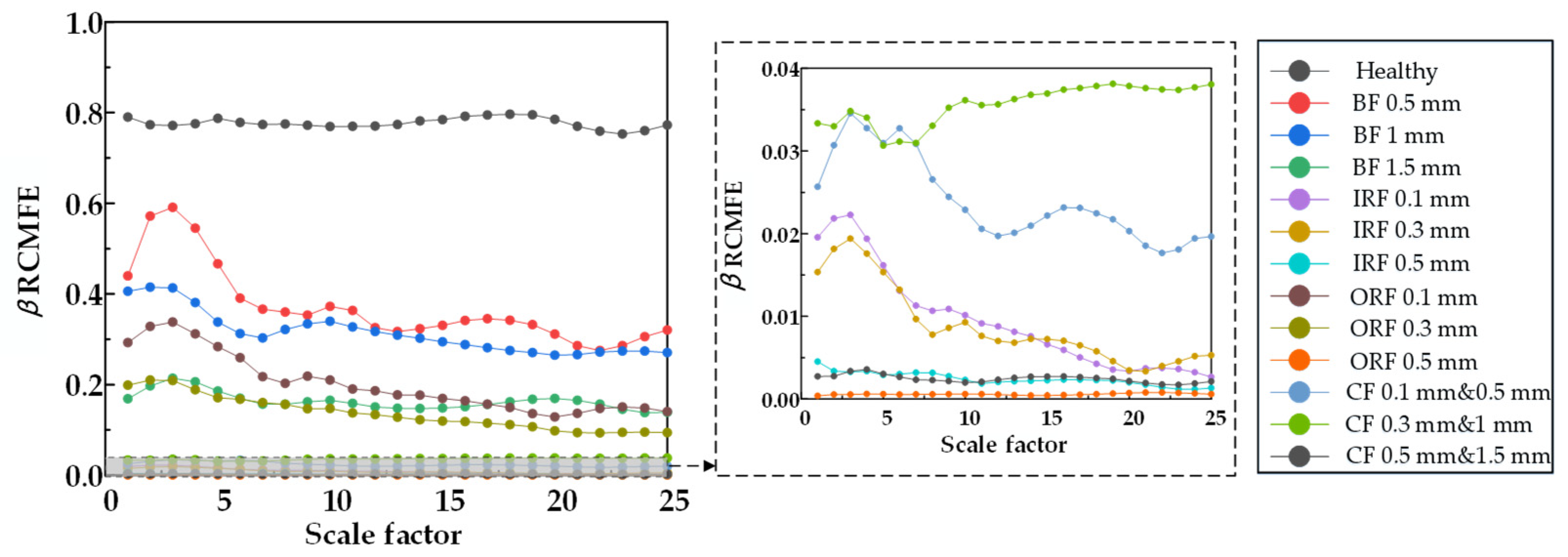
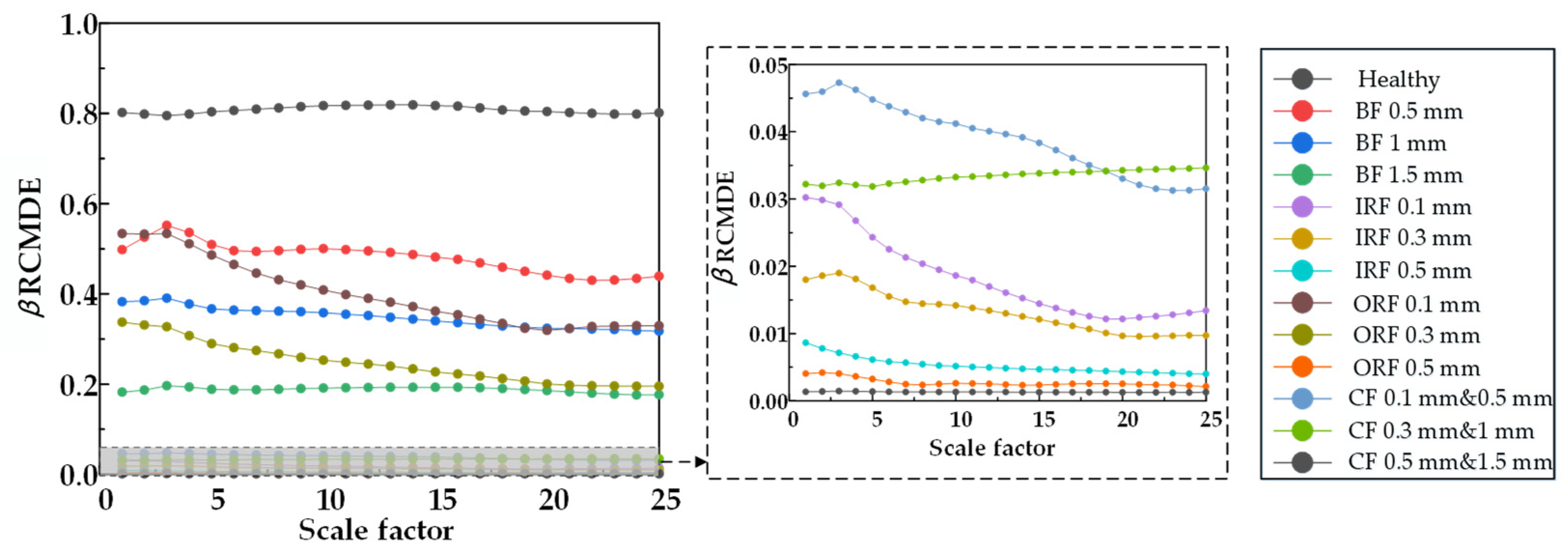
From Figure 20, Figure 21 and Figure 22, RCMSE, RCMFE, and RCMDE cannot distinguish the normal state from the abnormal state in the first five scales, and different fault entropy values overlap and cannot keep local stability. From Figure 23, Figure 24 and Figure 25, for α RCMSE, α RCMFE, and α RCMDE, we can see that the entropy values of normal and other faults did not coincide on the whole scale factor. With an increase in scale factor, the entropy values of normal and abnormal states could be clearly distinguished; however, α RCMSE, α RCMFE, and α RCMDE presented the problem of aliasing between fault signals, which can lead to the problem that the fault type of the bearing is difficult to identify. From Figure 26, Figure 27 and Figure 28, it can be seen that β RCMSE, β RCMFE, and β RCMDE could not coincide with other fault entropy values on the whole scale factor. With an increase in scale factor, the difference between normal and abnormal entropy was more obvious. When weighted by the double characteristic parameters β RCMSE, β RCMFE, and β RCMDE, compared with the entropy weighted by single characteristic parameters, the distance between normal and abnormal entropy values was larger. The overlap between different entropy values was reduced and the stability under a multi-scale state was maintained as much as possible. It can be seen, from Figure 29, Figure 30, Figure 31 and Figure 32 that γ RCMSE, γ RCMFE, γ RCMDE, and ω RCMWE could not coincide with other fault entropy values on the whole scale factor. With an increase in scale factor, the normal and abnormal entropy values could be clearly distinguished. When weighted by multiple characteristic parameters, γ RCMSE, γ RCMFE, γ RCMDE, and ω RCMWE, compared with the single and double characteristic parameter weighted parameters, the entropy value method presented more obvious differentiation between normal and abnormal entropy values, ensuring that different entropy values do not overlap and maintaining their stability in multi-scale state. Therefore, the weighted entropy method with multiple characteristic parameters could better identify the fault types of bearings under different faults and damage conditions at any scale. In terms of fault categories, classification is easy to achieve, different fault types can be clearly and correctly identified, and entropy values between different fault types do not overlap. According to the degradation degree of different faults, the entropy value changed exponentially with an increase in the scale factor.
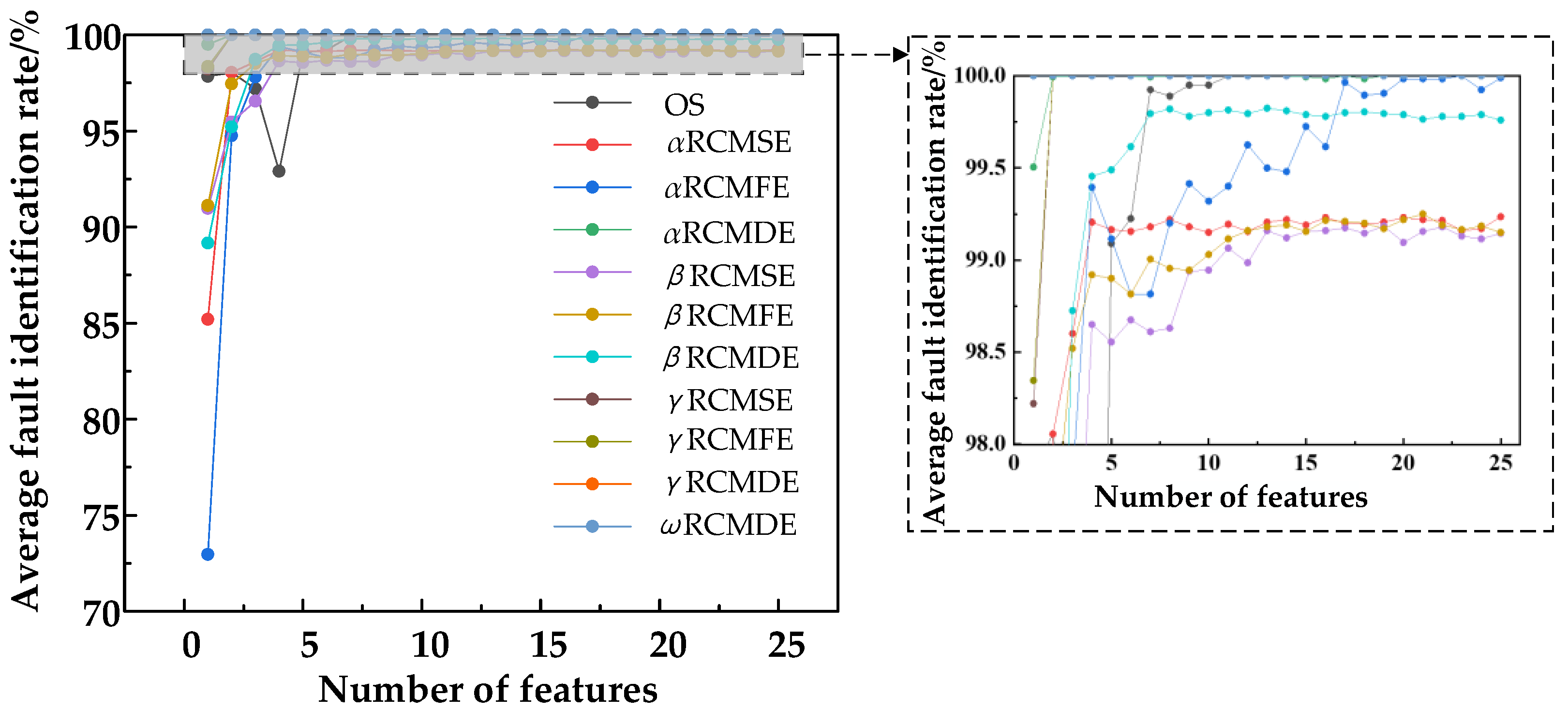
To further quantify the feature extraction effect of the ω RCMWE method, the 11 feature sets of the OS, α RCMSE, α RCMFE, α RCMDE, β RCMSE, β RCMFE, β RCMDE, γ RCMSE, γ RCMFE, γ RCMDE, and ω RCMWE, were, respectively used to extract 1 to 25 features from the initial features, which were used as input to the classifier as training and testing samples, in order to achieve fault classification and recognition. A total of 40 groups of samples under 13 working conditions were randomly selected for training, and the remaining 160 groups of samples were tested. There were 520 training samples, 2080 testing samples, and 50 cyclic tests for rolling bearings under 13 working conditions. The training samples and training tags were input into the multi-class classifier based on SVM for training, and a model containing fault feature information was obtained after training. The classifier used this model to analyze the test samples, which can realize fault diagnosis by comparing the output results of the classifier with the actual results. The SVM classifier obtained the bearing fault recognition results from the 11 feature extraction methods, as shown in Figure 33.
We can see that the original time–frequency domain feature OS decreased with the increase in the number of features, then increased along with the number of features. After weighting the first sensitive feature, for α RCMSE the recognition accuracy was 82.75%; for α RCMFE, the recognition accuracy was 87.46%; and, for α RCMDE, the recognition accuracy was 84.44%. After weighting the second sensitive feature, for β RCMSE, the recognition accuracy was 87.74%; for β RCMFE, the recognition accuracy was 86.75%; and for β RCMDE, the recognition accuracy was 86.21%. The analysis indicated that the minimum diagnostic accuracy under the first feature was 82.75%. For α RCMSE, α RCMFE, α RCMDE, β RCMSE, β RCMFE, and β RCMDE, with an increase in the scale factor, the fault accuracy rate increased, and the overall fault identification rate could be guaranteed to be above 82.75%. For γ RCMSE, γ RCMFE, and γ RCMDE, the fault accuracy also increased with an increase in the scale factor, and the overall fault identification rate was above 90.32%. Therefore, the observed rule was that the fault recognition rate decreases with an increase in the scale factor, which indicates that the recognition rate will not increase with the increase in the scale factor but, instead, will decrease with an increase in the amount of redundant information. The results of the ω RCMWE and γ RCMDE method were better than those of the other methods: from the first eigenvalue, it was found that the fault identification rate of the method based on ω RCMWE and γ RCMDE reached 92.22%. Thus, this method can identify the fault types of bearings under different damage conditions at any scale, and the fault identification rate is more stable than that of other methods. The first scale factors for α RCMSE, α RCMFE, α RCMDE, β RCMSE, β RCMFE, and β RCMDE showed a decrease in the fault recognition rate, mainly due to the influence of the weighting index. This makes the difference between normal and abnormal entropy larger, and enhances the influence of entropy. The above analysis indicated that the proposed method based on ω RCMWE and γ RCMDE is superior to other methods for fault diagnosis in bearing experimental data.
The results showed that the fault identification rate based on the ω RCMWE method can reach 92.22%, according to the first feature number. Therefore, the method can identify the fault types of bearings in different damage states at any scale, the fault identification rate is more stable than that of other methods, and the weighted entropy method is better than the established entropy methods at all scales, in terms of estimating the complexity of the signal correctly. The weighted entropy method can identify the normal and abnormal states of the bearing, different fault states can be distinguished better, and composite fault states can also be distinguished. This method can retain the different fault categories within a certain range and there is no overlap between them, indicating that the clustering performance between different fault categories is good. Therefore, entropy can be used to describe the complexity of vibration signals of rolling bearings, as a characteristic index to distinguish different fault types and damage degrees of rolling bearings. The entropy weighting process should follow the following two principles, as far as possible: 1. The trend of the selected indicators should be consistent with the entropy change law (i.e., meeting the monotonicity) and, in principle, should meet the rule of the bearing failure mechanism. The real bearing damage mechanism is that when the rolling bearing works in a healthy state, the vibration is random. Once the rolling bearing fails, the failed part will become the driving source, which will produce regular and periodic impact. Therefore, the obtained vibration signal has obvious regularity and self-similarity increases. When a fault occurs, the vibration signal of the system has obvious impact characteristics, and different fault locations have different fault characteristic frequencies, so the faults in different locations will lead to different complexity of the vibration signal. Because the outer ring is fixed, the signal transmission path measured by the sensor on the rolling bearing seat is the shortest. When the outer ring fails, the impact characteristic frequency of the vibration signal is single and simple. In addition, compared with the failure of the inner ring and ball element, the characteristic frequency of outer ring failure is the smallest, so its self-similarity and regularity are also the most obvious. Because the inner ring rotates with the shaft, and the rolling elements rotate and revolve around the shaft, the fault characteristic frequency of the ball is higher than that of the inner and outer rings, the rolling vibration signal rolling element fault is more complicated than that of the inner and outer rings; 2. With an increase in damage depth, the amplitude of signal increases, and the impact law of signal is more obvious. Therefore, the entropy value should decrease with an increase in bearing damage depth, and the normal entropy value should be the maximum. The entropy value for judging the fault types of rolling bearings should conform to the rule that the normal entropy value is greater than the ball fault entropy value, the ball fault entropy value is greater than the inner race fault entropy value, and the inner race fault entropy value is greater than the outer race fault entropy value. The judgment of bearing damage state should conform to the rule that mild damage state is greater than moderate damage state, and moderate damage state is greater than severe damage state. Therefore, the weighted entropy method proposed in this paper can be used as a new indicator for rolling bearing health monitoring, in order to judge whether a bearing is abnormal or not, thus laying a theoretical foundation for the healthy operation and maintenance of rotating machinery.
5. Conclusions

In this paper, a new method of weak signal feature extraction for rolling bearings based on refined composite multi-scale weighted entropy was proposed. In the pro-posed method, the time–frequency domain features were constituted into a multi-dimensional original fault feature set, and the feature sensitivity was evaluated using four types of feature evaluation criteria. Next, the optimal feature subset was filtered according to the specific feature evaluation criteria, from which the sensitive feature parameters are constructed and used as the weighting parameters for the re-fined composite multi-scale weighted entropy. The influence of the combination of weighted parameters on the fault degree of rolling bearings was determined through two experimental verification analysis groups. The fault recognition rate reached 100% and 92.22%, respectively, based on the RCMWE method, starting from the first number of features. The weighted entropy method showed a better ability to correctly estimate the signal complexity at all scales than the established entropy methods, and could effectively distinguish between health and fault states. In addition, the proposed method was able to generate enhanced feature vectors, thus providing a higher classification accuracy when estimating bearing fault types and fault severity. The weighted entropy can be used as an alarm threshold for monitoring early abnormal faults, as well as to determine the degree of degradation damage in a bearing. In practical engineering applications, the common forms of bearing failure are not certain and the form of failure is often random. It is possible for a single or compound failure to occur in a bearing. Bearing damage often does not occur instantaneously, but gradually due to the accumulation of time. Therefore, the significance of developing a new bearing damage indicator is first to determine when a bearing failure occurs. The second point is to determine what kind of bearing failure has occurred. The third point is to determine the severity of the occurrence of the failure. In future research, the entropy method can well detect the dynamic changes of rotating machinery. The combination of entropy and machine learning method can provide a promising tool for fault diagnosis of rotating machinery. The fault diagnosis of rotating machinery faces the challenge of variable speed. It is of great significance to complete the entropy method in fault diagnosis of rotating machinery under variable speed conditions.
Author Contributions

J.G. conceived the research; D.X. and Y.W. performed the experiments and wrote the paper; Y.F. and J.S. guided experiments and contributed to revising the paper; D.X. and F.W. provided software support and data analysis. All authors have read and agreed to the published version of the manuscript.

Funding

This research was funded by the National Natural Science Foundation of China, grant number 52175502.

Institutional Review Board Statement

Not applicable.

Informed Consent Statement

Not applicable.

Data Availability Statement

Not applicable.

Conflicts of Interest

The authors declare no conflict of interest.

References

  1. Zou, L.; Li, Y.; Xu, F. An adversarial denoising convolutional neural network for fault diagnosis of rotating machinery under noisy environment and limited sample size case. Neurocomputing 2020, 407, 105–120. [Google Scholar] [CrossRef]
  2. Lei, Y.; Yang, B.; Jiang, X.; Jia, F.; Li, N.; Nandi, A.K. Applications of machine learning to machine fault diagnosis: A review and roadmap. Mech. Syst. Signal Process. 2020, 138, 106587. [Google Scholar] [CrossRef]
  3. Randall, R.B.; Antoni, J. Rolling element bearing diagnostics-A tutorial. Mech. Syst. Signal Process. 2011, 25, 485–520. [Google Scholar] [CrossRef]
  4. Liang, K.; Zhao, M.; Lin, J.; Ding, C.; Jiao, J.; Zhang, Z. A novel indicator to improve fast kurtogram for the health monitoring of rolling bearing. IEEE Sens. J. 2020, 20, 12252–12261. [Google Scholar] [CrossRef]
  5. Caesarendra, W.; Tjahjowidodo, T. A review of feature extraction methods in vibration-based condition monitoring and its application for degradation trend estimation of low-speed slew bearing. Machines 2017, 5, 21. [Google Scholar] [CrossRef]
  6. Igba, J.; Alemzadeh, K.; Durugbo, C.; Eiriksson, E.T. Analysing RMS and peak values of vibration signals for condition monitoring of wind turbine gearboxes. Renew. Energy 2016, 91, 90–106. [Google Scholar] [CrossRef] [Green Version]
  7. Li, Y.; Li, H.; Wang, B.; Yu, H.; Wang, W. Research on the feature selection of rolling bearings’ degradation features. Shock. Vib. 2019, 2019, 6450719. [Google Scholar] [CrossRef] [Green Version]
  8. Laissaoui, A.; Bouzouane, B.; Miloudi, A.; Hamzaoui, N. Perceptive analysis of bearing defects (Contribution to vibration monitoring). Appl. Acoust. 2018, 140, 248–255. [Google Scholar] [CrossRef]
  9. Sassi, S.; Badri, B.; Thomas, M. TALAF and THIKAT as innovative time domain indicators for tracking BALL bearings. In Proceedings of the 24th Seminar on Machinery Vibration, Canadian Machinery Vibration Association, Montreal, QC, Canada, 25–27 October 2006. [Google Scholar]
  10. Logan, D.; Mathew, J. Using the correlation dimension for vibration fault diagnosis of rolling element bearings—I. Basic concepts. Mech. Syst. Signal Process. 1996, 10, 241–250. [Google Scholar] [CrossRef]
  11. Guo, Q.; Li, Y. Early Fault Diagnosis of Rolling Bearing Based on Lyapunov Exponent. In Proceedings of the 2018 International Symposium on Power Electronics and Control Engineering (ISPECE 2018), Xi’an, China, 28–30 December 2018. [Google Scholar]
  12. Yang, J.; Zhang, Y.; Zhu, Y. Intelligent fault diagnosis of rolling element bearing based on SVMs and fractal dimension. Mech. Syst. Signal Process. 2007, 21, 2012–2024. [Google Scholar] [CrossRef]
  13. Pincus, S.M. Approximate entropy as a measure of system complexity. Proc. Natl. Acad. Sci. USA 1991, 88, 2297–2301. [Google Scholar] [CrossRef] [PubMed] [Green Version]
  14. Richman, J.S.; Moorman, J.R. Physiological time-series analysis using approximate entropy and sample entropy. Am. J. Physiol.-Heart Circ. Physiol. 2000, 278, H2039–H2049. [Google Scholar] [CrossRef] [PubMed] [Green Version]
  15. Delgado-Bonal, A.; Marshak, A. Approximate entropy and sample entropy: A comprehensive tutorial. Entropy 2019, 21, 541. [Google Scholar] [CrossRef] [PubMed] [Green Version]
  16. Chen, W.; Zhuang, J.; Yu, W.; Wang, Z. Measuring complexity using FuzzyEn, ApEn, and SampEn. Med. Eng. Phys. 2009, 31, 61–68. [Google Scholar] [CrossRef] [PubMed]
  17. Bandt, C.; Pompe, B. Permutation entropy: A natural complexity measure for time series. Phys. Rev. Lett. 2002, 88, 174102. [Google Scholar] [CrossRef]
  18. Rostaghi, M.; Azami, H. Dispersion Entropy: A Measure for Time-Series Analysis. IEEE Signal Process. Lett. 2016, 23, 610–614. [Google Scholar] [CrossRef]
  19. Costa, M.; Goldberger, A.L.; Peng, C.K. Multiscale entropy analysis of complex physiologic time series. Phys. Rev. Lett. 2002, 89, 068102. [Google Scholar] [CrossRef] [Green Version]
  20. Liu, H.; Han, M. A fault diagnosis method based on local mean decomposition and multi-scale entropy for roller bearings. Mech. Mach. Theory 2014, 75, 67–78. [Google Scholar] [CrossRef]
  21. Minhas, A.S.; Sharma, N.; Kankar, P.; Singh, S. A comparative study for the selection of an entropy technique to classify bearing faults. In Proceedings of the 2019 IEEE International Conference on Electrical, Computer and Communication Technologies (ICECCT), Coimbatore, India, 20–22 February 2019. [Google Scholar]
  22. Zhao, D.; Liu, S.; Cheng, S.; Sun, X.; Wang, L.; Wei, Y.; Zhang, H. Parallel multi-scale entropy and it’s application in rolling bearing fault diagnosis. Measurement 2021, 168, 108333. [Google Scholar] [CrossRef]
  23. Zhu, K.; Chen, L.; Hu, X. A multi-scale fuzzy measure entropy and infinite feature selection based approach for rolling bearing fault diagnosis. J. Nondestruct. Eval. 2019, 38, 90. [Google Scholar] [CrossRef]
  24. Li, H.; Huang, J.; Yang, X.; Luo, J.; Zhang, L.; Pang, Y. Fault diagnosis for rotating machinery using multiscale permutation entropy and convolutional neural networks. Entropy 2020, 22, 851. [Google Scholar] [CrossRef] [PubMed]
  25. Yan, X.A.; Jia, M.P. Intelligent fault diagnosis of rotating machinery using improved multiscale dispersion entropy and mRMR feature selection. Knowl.-Based Syst. 2019, 163, 450–471. [Google Scholar] [CrossRef]
  26. Wang, Z.; Yao, L.; Cai, Y. Rolling bearing fault diagnosis using generalized refined composite multiscale sample entropy and optimized support vector machine. Measurement 2020, 156, 107574. [Google Scholar] [CrossRef]
  27. Xu, F.; Tse, P.W. A method combining refined composite multiscale fuzzy entropy with PSO-SVM for roller bearing fault diagnosis. J. Cent. South Univ. 2019, 26, 2404–2417. [Google Scholar] [CrossRef]
  28. Humeau-Heurtier, A.; Wu, C.-W.; Wu, S.-D. Refined composite multiscale permutation entropy to overcome multiscale permutation entropy length dependence. IEEE Signal Process. Lett. 2015, 22, 2364–2367. [Google Scholar] [CrossRef]
  29. Luo, S.; Yang, W.; Luo, Y. Fault diagnosis of a rolling bearing based on adaptive sparest narrow-band decomposition and Refined Composite multiscale dispersion entropy. Entropy 2020, 22, 375. [Google Scholar] [CrossRef] [PubMed] [Green Version]
  30. Zhang, L.; Huang, W.; Xiong, G. Assessment of rolling element bearing fault severity using multi-scale entropy. J. Vib. Shock. 2014, 33, 185–189. [Google Scholar]
  31. Zheng, J.; Dong, Z.; Pan, H.; Ni, Q.; Liu, T.; Zhang, J. Composite multi-scale weighted permutation entropy and extreme learning machine based intelligent fault diagnosis for rolling bearing. Measurement 2019, 143, 69–80. [Google Scholar] [CrossRef]
  32. Li, Y.; Dai, W.; Zhang, W. Bearing fault feature selection method based on weighted multidimensional feature fusion. IEEE Access 2020, 8, 19008–19025. [Google Scholar] [CrossRef]
  33. Ying, W.; Tong, J.; Dong, Z.; Pan, H.; Liu, Q.; Zheng, J. Composite multivariate multi-Scale permutation entropy and laplacian score based fault diagnosis of rolling bearing. Entropy 2022, 24, 160. [Google Scholar] [CrossRef]
  34. Minhas, A.S.; Kankar, P.; Kumar, N.; Singh, S. Bearing fault detection and recognition methodology based on weighted multiscale entropy approach. Mech. Syst. Signal Process. 2021, 147, 107073. [Google Scholar] [CrossRef]
  35. Li, Y.; Wang, X.; Liu, Z.; Liang, X.; Si, S. The entropy algorithm and its variants in the fault diagnosis of rotating machinery: A review. IEEE Access 2018, 6, 66723–66741. [Google Scholar] [CrossRef]
  36. Wu, S.-D.; Wu, C.-W.; Lin, S.-G.; Lee, K.-Y.; Peng, C.-K. Analysis of complex time series using refined composite multiscale entropy. Phys. Lett. A 2014, 378, 1369–1374. [Google Scholar] [CrossRef]
  37. Li, Y.; Miao, B.; Zhang, W.; Chen, P.; Liu, J.; Jiang, X. Refined composite multiscale fuzzy entropy: Localized defect detection of rolling element bearing. J. Mech. Sci. Technol. 2019, 33, 109–120. [Google Scholar] [CrossRef]
  38. Azami, H.; Rostaghi, M.; Abásolo, D.; Escudero, J. Refined composite multiscale dispersion entropy and its application to biomedical signals. IEEE Trans. Biomed. Eng. 2017, 64, 2872–2879. [Google Scholar] [PubMed] [Green Version]
  39. Chakraborty, M.; Mitra, D. A novel automated seizure detection system from EMD-MSPCA denoised EEG: Refined composite multiscale sample, fuzzy and permutation entropies based scheme. Biomed. Signal Process. Control. 2021, 67, 102514. [Google Scholar]
  40. Zhang, W.; Zhou, J. A comprehensive fault diagnosis method for rolling bearings based on refined composite multiscale dispersion entropy and fast ensemble empirical mode decomposition. Entropy 2019, 21, 680. [Google Scholar] [CrossRef] [Green Version]
  41. Ge, J.; Yin, G.; Wang, Y.; Xu, D.; Wei, F. Rolling-bearing fault-diagnosis method based on multimeasurement hybrid-feature evaluation. Information 2019, 10, 359. [Google Scholar] [CrossRef] [Green Version]
  42. Huo, Z.; Zhang, Y.; Shu, L.; Gallimore, M. A new bearing fault diagnosis method based on fine-to-coarse multiscale permutation entropy, laplacian score and SVM. IEEE Access 2019, 7, 17050–17066. [Google Scholar] [CrossRef]
  43. Lin, Y.; Hu, Q.; Liu, J.; Chen, J.; Duan, J. Multi-label feature selection based on neighborhood mutual information. Appl. Soft Comput. 2016, 38, 244–256. [Google Scholar] [CrossRef]
  44. Sun, L.; Wang, T.; Ding, W.; Xu, J.; Lin, Y. Feature selection using Fisher score and multilabel neighborhood rough sets for multilabel classification. Inf. Sci. 2021, 578, 887–912. [Google Scholar] [CrossRef]
  45. Case Western Reserve University Bearing Data Center Website. Available online: http://csegroups.case.edu/bearingdatacenter/home (accessed on 26 June 2022).
  46. Chih-Chung, C.; Chih-Jen, L. LIBSVM: A library for support vector machines. ACM Trans. Intell. Syst. Technol. 2001, 2, 1–27. [Google Scholar] [CrossRef]
Figure 1. RCMWE characteristic index construction process.
Machines 10 01155 g001
Figure 2. Bearing test bench of CWRU.
Machines 10 01155 g002
Figure 3. Time-frequency domain waveforms of vibration acceleration signal and spectrums of rolling bearing under ten kinds of work conditions. (a) Time domain waveforms under 10 conditions; (b) spectrums under 10 conditions.
Machines 10 01155 g003
Figure 4. RCMSE entropy values of 25 scale factors under different damage degrees.
Machines 10 01155 g004
Figure 5. RCMFE entropy values of 25 scale factors under different damage degrees.
Machines 10 01155 g005
Figure 6. RCMDE entropy values of 25 scale factors under different damage degrees.
Machines 10 01155 g006
Figure 7. α RCMSE entropy values of 25 scale factors under different damage degrees.
Machines 10 01155 g007
Figure 8. α RCMFE entropy values of 25 scale factors under different damage degrees.
Machines 10 01155 g008
Figure 9. α RCMDE entropy values of 25 scale factors under different damage degrees.
Machines 10 01155 g009
Figure 10. β RCMSE entropy values of 25 scale factors under different damage degrees.
Machines 10 01155 g010
Figure 11. β RCMFE entropy values of 25 scale factors under different damage degrees.
Machines 10 01155 g011
Figure 12. β RCMDE entropy values of 25 scale factors under different damage degrees.
Machines 10 01155 g012
Figure 13. γ RCMSE entropy values of 25 scale factors under different damage degrees.
Machines 10 01155 g013
Figure 14. γ RCMFE entropy values of 25 scale factors under different damage degrees.
Machines 10 01155 g014
Figure 15. γ RCMDE entropy values of 25 scale factors under different damage degrees.
Machines 10 01155 g015
Figure 16. ω RCMWE entropy values of 25 scale factors under different damage degrees.
Machines 10 01155 g016
Figure 17. Bearing fault identification rate under different number of features.
Machines 10 01155 g017
Figure 18. Rolling Bearing Fault Diagnosis Test Bench.
Machines 10 01155 g018
Figure 19. Time−frequency domain waveforms of rolling bearing under 13 kinds of work conditions. (a) Time domain waveforms under 13 conditions; (b) spectrums under 13 conditions.
Machines 10 01155 g019
Figure 20. RCMSE entropy values of 25 scale factors under different damage degrees.
Machines 10 01155 g020
Figure 21. RCMFE entropy values of 25 scale factors under different damage degrees.
Machines 10 01155 g021
Figure 22. RCMDE entropy values of 25 scale factors under different damage degrees.
Machines 10 01155 g022
Figure 23. α RCMSE entropy values of 25 scale factors under different damage degrees.
Machines 10 01155 g023
Figure 24. α RCMFE entropy values of 25 scale factors under different damage degrees.
Machines 10 01155 g024
Figure 25. α RCMDE entropy values of 25 scale factors under different damage degrees.
Machines 10 01155 g025
Figure 26. β RCMSE entropy values of 25 scale factors under different damage degrees.
Machines 10 01155 g026
Figure 27. β RCMFE entropy values of 25 scale factors under different damage degrees.
Machines 10 01155 g027
Figure 28. β RCMDE entropy values of 25 scale factors under different damage degrees.
Machines 10 01155 g028
Figure 29. γ RCMSE entropy values of 25 scale factors under different damage degrees.
Machines 10 01155 g029
Figure 30. γ RCMFE entropy values of 25 scale factors under different damage degrees.
Machines 10 01155 g030
Figure 31. γ RCMDE entropy values of 25 scale factors under different damage degrees.
Machines 10 01155 g031
Figure 32. ω RCMWE entropy values of 25 scale factors under different damage degrees.
Machines 10 01155 g032
Figure 33. Bearing fault identification rate under different number of features.
Machines 10 01155 g033
Table 1. Characteristic indices in time–frequency domain.
SymbolsFormulaSymbolsFormulaSymbolsFormula
x p , 1 max ( | u p , i | ) x p , 6 i = 1 L ( u p , i x p , 2 ) 4 L ( x p , 3 ) x p , 11 1 Q a = 1 Q w a
x p , 2 1 L i = 1 L u p , i x p , 7 x p , 4 x p , 2 x p , 12 a = 1 Q f a w a a = 1 Q w a
x p , 3 1 L i = 1 L ( u p , i x p , 2 ) 2 x p , 8 x p , 1 x p , 4 x p , 13 a = 1 Q w a ( f a ) 2 a = 1 Q w a
x p , 4 i = 1 L ( u p , i ) 2 L x p , 9 x p , 1 x p , 3 x p , 14 a = 1 Q w a ( f a x p , 12 ) 2 Q
x p , 5 i = 1 L ( u p , i x p , 2 ) 3 L ( x p , 3 ) 3 x p , 10 x p , 1 1 L i = 1 L | u p , i | 2 x p , 15 a = 1 Q w a ( f a x p , 12 ) 4 Q ( x p , 14 ) 2
Table 2. The 6205 bearing parameters and failure frequency.
Outer Diameter/mmInner Diameter/mmSection Circle Diameter/mmNumber of BallsBall Diameter/mm
522539.0497.94
Frequency Shift /HzInner Race Frequency/HzOuter Race Frequency/HzBall Frequency/Hz
29.95162.1857107.364370.5846
Table 3. Experimental parameter settings under different fault conditions.
Experiment NumberBearing StateSample GroupsSample Points
No. 1Healthy502048
No. 2IRF 0.007inch502048
No. 3IRF 0.014inch502048
No. 4IRF 0.021inch502048
No. 5ORF 0.007inch502048
No. 6ORF 0.014inch502048
No. 7ORF 0.021inch502048
No. 8BF 0.007inch502048
No. 9BF 0.014inch502048
No. 10BF 0.021inch502048
Table 4. Evaluation score of four types of characteristics.
Feature ParametersLSPSFSMI
x 1 4.8323 × 10−30.690669.42022.1079
x 2 2.6411 × 10−30.7113142.65822.2944
x 3 2.6455 × 10−30.7127143.24502.2203
x 4 9.2979 × 10−30.2501145.38571.3639
x 5 1.0484 × 10−30.53524904.48142.1803
x 6 1.1424 × 10−30.5237607.83782.4437
x 7 1.4550 × 10−30.6058917.82922.3220
x 8 9.0703 × 10−40.54362243.19532.4539
x 9 6.0021 × 10−40.66672939.33712.4267
x 10 1.0483 × 10−30.53524903.93112.1802
x 11 5.1100 × 10−20.20323.50101.2861
x 12 2.2474 × 10−40.66392105.54962.0344
x 13 0.76390.035400.0161
x 14 4.2465 × 10−40.69594297.39392.5040
x 15 1.1891 × 10−40.6064791.57582.5113
Table 5. Feature rankings under different methods.
MethodFeature Ranking
LS x 15 < x 12 < x 14 < x 9 < x 8 < x 10 < x 5 < x 6 < x 7 < x 2 < x 3 < x 1 < x 4 < x 11 < x 13
PS x 3 > x 2 > x 14 > x 1 > x 9 > x 12 > x 15 > x 7 > x 8 > x 5 > x 10 > x 6 > x 4 > x 11 > x 13
FS x 5 > x 10 > x 14 > x 9 > x 8 > x 12 > x 7 > x 15 > x 6 > x 4 > x 3 > x 2 > x 1 > x 11 > x 13
MI x 15 > x 14 > x 8 > x 6 > x 9 > x 7 > x 2 > x 3 > x 5 > x 10 > x 1 > x 12 > x 4 > x 11 > x 13
Table 6. ER-16K bearing parameters and failure frequency.
Outer Diameter/mmInner Diameter/mmSection Circle Diameter/mmNumber of BallsBall Diameter/mm
51.612825.438.506497.9375
Speed/r/minFrequency Shift /HzInner Race Frequency/HzOuter Race Frequency/HzBall Frequency/HzCage Frequency/Hz
240040217.1042142.895892.901315.8773
Table 7. Test parameters for 13 different fault states.
Experiment NumberBearing StateSample GroupsSample Points
No. 1Healthy1032768
No. 2BF 0.5 mm1032768
No. 3BF 1 mm1032768
No. 4BF 1.5 mm1032768
No. 5IRF 0.1 mm1032768
No. 6IRF 0.3 mm1032768
No. 7IRF 0.5 mm1032768
No. 8ORF 0.1 mm1032768
No. 9ORF 0.3 mm1032768
No. 10ORF 0.5 mm1032768
No. 11CF 0.1 mm&0.5 mm1032768
No. 12CF 0.3 mm&1 mm1032768
No. 13CF 0.5 mm&1.5 mm1032768
Table 8. Scoring results for the four types of evaluation characteristics.
Feature ParametersLSPSFSMI
x 1 0.0010.604316,580.13602.7041
x 2 5.7254 × 10−40.62702077.29652.7296
x 3 5.7221 × 10−40.62692128.32442.7225
x 4 0.01480.272063.33331.995
x 5 0.00380.35755610.47472.4470
x 6 0.00740.6185922.04772.5882
x 7 0.03460.400224.84281.7944
x 8 0.00460.5934975.96662.0774
x 9 0.01230.362585.99462.0174
x 10 0.00380.35755610.47472.4470
x 11 3.1455 × 10−40.64458496.72092.7374
x 12 0.00680.6473121.49372.5057
x 13 8.3269 × 10−40.466029.34302.5055
x 14 2.3983 × 10−40.64793563.05502.8507
x 15 9.5751 × 10−50.6426621.93342.8327
Table 9. Sorted features.
MethodFeature Sorting
LS x 15 < x 14 < x 11 < x 3 < x 2 < x 13 < x 1 < x 5 < x 10 < x 8 < x 12 < x 6 < x 9 < x 4 < x 7
PS x 14 > x 12 > x 11 > x 15 > x 2 > x 3 > x 6 > x 1 > x 8 > x 13 > x 7 > x 9 > x 10 > x 5 > x 4
FS x 1 > x 11 > x 10 > x 5 > x 14 > x 3 > x 2 > x 8 > x 6 > x 15 > x 12 > x 9 > x 4 > x 13 > x 7
MI x 14 > x 15 > x 11 > x 2 > x 3 > x 1 > x 6 > x 12 > x 13 > x 5 > x 10 > x 8 > x 9 > x 4 > x 7
Publisher’s Note: MDPI stays neutral with regard to jurisdictional claims in published maps and institutional affiliations.