Article

Sensor Distribution Optimization for Composite Impact Monitoring Based on AR Model and LPP

1
School of Mechatronics & Vehicle Engineering, East China Jiaotong University, Nanchang 330013, China
2
Key Laboratory of Conveyance Equipment, East China Jiaotong University, Ministry of Education, Nanchang 330013, China
*
Author to whom correspondence should be addressed.
Machines 2022, 10(12), 1154; https://doi.org/10.3390/machines10121154
Submission received: 29 October 2022 / Revised: 26 November 2022 / Accepted: 28 November 2022 / Published: 2 December 2022

Abstract

:
The aim of this article is to provide a sensor distribution optimization method for the effective impact monitoring of composite plates with fewer sensors. In this research, the number of sensors and the minimum difference between categories are used as objective functions I and II, respectively, where the minimum difference is the Euclidean distance between different influence categories. The dual objective functions are defined by means of finite element analysis, the autoregressive (AR) model, and locality−preserving projection (LPP). The sensor distribution is optimized based on Multi−Objective Particle Swarm Optimization (MOPSO). Finally, an impact monitoring method is provided, and an experimental platform is built to verify the method. According to the optimization results, different grid sizes have a certain impact on the identification results, with the smaller the grid size, the smaller the minimum difference between categories. Within a given grid size, the minimum difference between categories increases with the increasing number of sensors. Experiments show that the higher the number of sensors, the higher the recognition rate of the system. Comparing the experimental results with the energy analysis of wavelet bands and PCA methods, it is found that the method used in this study has a higher recognition rate. This research provides an impact monitoring method based on sensor distribution optimization. And the effectiveness of the method is verified by experiments. It provides a useful reference and choice for the structure condition monitoring of composite material plates.

1. Introduction

During the service period, due to continuous environmental erosion, various loads and natural disasters, the state of a composite structure tends to deteriorate, and the damage is not easily detected. At the same time, because composites are mostly anisotropic and mainly used to resist tensile deformation, the impact resistance is generally poor, especially for low−speed impact. Therefore, real−time monitoring of composite structures and accurate judgment of the degree and location of the impact on composite structures is an important technical guarantee for the safe service of composite structures.
In recent years, many scholars have studied the impact monitoring of composite plate structures. Park obtains the time delay of each impact signal by arranging sensors at the four corners of the composite plate, and realizes the impact location by using a neural network [1]. After all impact signals are normalized by Pratik et al., the database is established, and then the random impact location of the composite wing is realized by using the correlation coefficient method and the root mean square method, respectively [2]. Lukasz uses nonlinear vibration acoustic modulation technology to detect the impact damage of composite sandwich plates [3]. Guo uses FBG sensors for impact detection and proposed an algorithm based on wavelet packet energy eigenvectors and similarity matching to realize impact location [4]. Li proposes the use of the Teager energy operator to process the impact signal and locate the low−speed impact loads of wing structures [5]. Gao provides a new idea for the health monitoring of composite structures based on the use of an ultrasonic guided wave to monitor the tensile fatigue damage of composite materials [6].
The optimization of sensor distribution in structural health monitoring is a research focus. Wu et al. proposed an improved artificial fish swarm algorithm to realize the optimal selection of structure sensor position [7]. The optimization of sensor networks requires a reduction in the number of sensors and increased monitoring accuracy. Thus, it is a multi−objective optimization problem (MOOP). Inherently, sensor location and number are two conflicting goals for the design of sensor networks. In previous studies, in order to solve the MOOP, many researchers improved the initial heuristic algorithm. Modern heuristic algorithms include the particle swarm optimization algorithm (PSO) [8], genetic algorithm (GA) [9,10], simulated annealing (SA) [11], monkey algorithm (MA) [12], ant colony algorithm (ACO) [13], and differential evolution (DE). Kim established a novel particle swarm optimization framework to achieve robust consensus of decentralized sensors with neighbors rather than through centralized control [14]. An algorithm based on ladder diffusion and ACO is proposed to solve the power consumption and transmission routing problems in wireless networks. Céspedes−Mota uses an improved differential evolution algorithm to optimize the distribution of wireless sensor networks according to the distance between the sensors [15]. Reyes−Sierra proposes a multi−objective particle swarm optimization algorithm to solve the multi−objective optimization problem [16]. Chaudhry also uses this method to optimize the sensor network and realizes the search for an effective solution of an Internet of Things wireless sensor network without considering the complete search space [17]. Lu uses BIM to develop a component ballastless track structure health monitoring system to optimize the sensor installation and monitoring program [18]. Lu proposed a method based on energy spectral density to extract damage-sensitive features of vehicle−induced dynamic response signals for long−term monitoring and evaluation of structural vibration responses [19].
Past research focused on impact monitoring tended to have a single goal, focusing primarily on hardware (sensor network) or software (monitoring algorithm), ignoring the cooperation between them. However, combining the monitoring algorithm and the distribution optimization of sensor networks to realize the cooperation of software and hardware is expected to provide an effective new way for impact monitoring. In this paper, the beginning of Section 2 describes the problem. The number of sensors and the minimum difference among categories are taken as objective functions I and II, respectively. Section 2.2 describes how to use finite element analysis, the AR model, and LPP to define objective function II. In Section 3, MOPSO is used to optimize the algorithm. Through optimization, different degrees of Pareto solution sets can be obtained. In Section 4, the effects of grid size and sensor location on sensor distribution optimization are studied and demonstrated experimentally. Finally, the paper is concluded in Section 5.

2. Optimization Problems

The purpose of impact monitoring is to distinguish different types of impact. In this paper, the impact category is defined as the impact locations under different impact degrees, in which the impact locations and the preset sensor points are defined by the intersection of the grid lines of the composite plate. Thus, the optimization problems of sensor distribution optimization include:
  • Minimizing the number of sensors.
  • Maximizing the effect of state detection.

2.1. Objective Function I: Number of Sensors

The number of sensors refers to the number of sensors arranged on the monitored object. Effectively reducing the number of sensors is conducive to improving data processing speed and reducing the cost of the system. Therefore, the number of sensors is set as objective function I.
In the research, for an n × n grid on a composite plate, there are a = n 1 2 alternative locations for sensors. The division diagram with n = 9   is shown in Figure 1. Each arrangement can be represented by a different combination of real numbers from 1 to a . The vector of the sensor distribution is:
S = S 1 , S 2 , , S l , l 1 , 2 , , a
where l is the number of sensors, that is, the objective function I. The element in S indicates the location of the sensor. For example, if the sensors are placed at locations 1 and 20, the vector S is equal to [1, 20] or [20, 1].

2.2. Objective Function II: Minimum Difference among Impact Categories

In order to maximize the impact monitoring effect, the optimization process is guided by the minimum difference among impact categories. In this research, b = a × a impact categories are obtained according to a impact locations and a ′ degrees, and the Euclidean distance among different categories is taken as the difference between the categories. The farther the minimum distance among b types of influence categories are, the better the effect of influence recognition under the sensor distribution scheme is. Therefore, the minimum distance between categories is defined as objective function II. For defining objective function II, finite element analysis is used to build a sample library, and then the AR model and LPP method are used to extract features and reduce dimensions. Finally, the distance between categories is calculated to find the objective function II. The specific process is as follows.

2.2.1. Impact Sample Library Based on Finite Element Simulation

In this paper, the composite material plate with the size of 15 mm × 500 mm × 500 mm is used as the tested object. The upper and lower surfaces of the composite plate are divided into 9 × 9 grids, and 64 nodes are generated on both surfaces. The node numbers are shown in Figure 1. Each node of the upper panel will be subject to two different degrees of low−speed impact, giving a total of 128 types of impact. Then, to obtain the response of all 128 types of impacts at each node of the lower panel, 128 × 64 types of impact response signals are generated in total.
The materials used in this study are epoxy resin/glass fiber (Epoxy30%/Gr70%) orthogonal anisotropic composite laminates. Because the model in the simulation is a simple rectangular structure, the Solid unit is chosen. And the interior of the composite material is a layered structure, so the Layered unit is chosen. In conclusion, a Solid Layered 46−bit simulation entity type is chosen. The unit type of the Solid model is defined, that is, a solid 46−layered structure is adopted.
The thickness of the composite plate is 15 mm, and there are 10 layers of laminates, each 1.5 mm thick. The internal structure of the laminates is an anisotropic orthogonal arrangement, and the layup form of the laminates is (0/90) s. For the accuracy of the experiment, the performance parameters of the composite plate in this study are set as shown in Table 1.
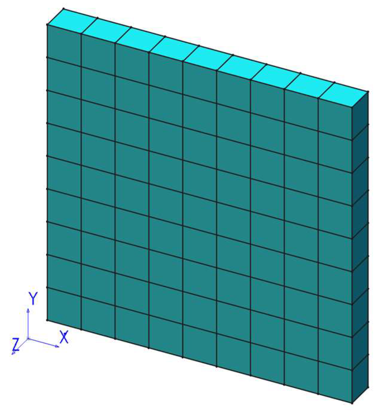
A mapping grid is used in ANSYS [20] because the laminate is a regular hexahedron. Considering that the front and rear surfaces are divided into 9 × 9 orthogonal distribution grids, eight sidelines are divided into nine segments, and four lateral edges are divided into one segment, as shown in Figure 2.
An impact simulation of the composite plate model was carried out to establish a sample library for the subsequent sensor optimization. In the simulation, full constraints are imposed on the nodes of the four segments of the composite plate to prevent the movement of the laminates from interfering with the impact response.
In the simulation, each node on the upper surface of the composite plate will be impacted to two different degrees, full−load impact and half−load impact. The full−load impact process is divided into two steps, the first load step is defined as 30 × sin ( 1744.4 × t ) ,   0 t 0.0018   s , which is divided into nine sub−load steps. In order to obtain the free impact response of the composite laminates, the second load step is empty load. The second load is divided into 991 sub−load steps. The process of half−load impact is consistent with that of full−load, but the applied force is smaller. The half−load impact function is defined as 15 × sin 1744.4 × t ,   0 t 0.0018   s .
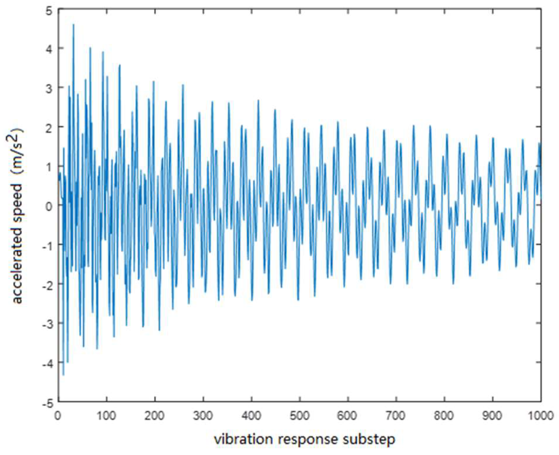
After the finite element analysis, a model is established and the mechanical model is solved by ANSYS software, the finite element calculation results of the simulated impact of the composite material plate can be viewed and analyzed by entering the TimeHist Postpro function of ANSYS. The degree of node displacement can be obtained by the TimeHist Postpro according to the graph. For example, the response of the 36th downside grid node is obtained as shown in Figure 3. The vibration response curve of the 36th downside grid node is obtained under the full−load impact to the 36th upside grid node.

2.2.2. Feature Extraction Based on AR Model

After obtaining the original simulation data, it is necessary to extract the features of the original data. The autoregressive parameters of the AR model are the most sensitive to the law of state change. In this model, the frequency−domain characteristics of the impact signal are described from statistics to obtain the frequency−domain characteristics of the original simulation data, and this model is widely used in the spectrum analysis of vibration signals [21,22]. Therefore, the AR model is used to estimate the power spectrum of the response signals under different impacts. The structure of the AR model can be described as follows:
k n = j = 1 p a j k n j + ε n , n = 1 , 2 , , a × b
Formula (2) is the AR model, wherein p is the order of the AR model, a j j = 1 , 2 , , p is the model parameter,   ε n is assumed to be equal to 0 on average, and k n is the sample data in the n th dimension after integration.
The AR model parameters a j   can be calculated from the autocorrelation sequence of the simulation data. According to the definition of an autocorrelation sequence, the autocorrelation function at time m is:
R x m = j = 1 p a j R x m j , m > 0 j = 1 p a j R x m j + σ w 2 , m = 0 m = 0 , 1 , , p
Formula (3) is expanded according to the matrix form, and based on the dual property of the autocorrelation function, which can be obtained as follows:
R X 0 R X 1 R X 2 R X 1 R X 0 R X 1 R X p R X p 1 R X p R X p 1 R X p 2 R X 0 1 a 1 a p = σ 2 0 0
The order of the AR model p is selected according to the Akaike information criterion (AIC) method [23]; the formula is:
A I C p = l o g σ p 2 + 2 p / N
where N is the number of samples and   σ p 2 is the prediction error of different−order model data.

2.2.3. Dimension Reduction Based on LPP

In order to make the calculation faster, the LPP method is used to reduce the dimension of the data [24]. The LPP method is an unsupervised linear dimension reduction method. Its basic idea is to map adjacent points in high−dimensional space to adjacent points in low−dimensional space by finding the projection direction matrix. It can effectively retain the inherent nonlinear structure and local characteristics of the original data. The principle is as follows:
The parameter a j   obtained by the AR model and the power spectrum obtained by coefficient filtering integrate into   X = x 1 , x 2 , , x p + 1 , through the projection matrix A , a set of vector−matrix Y = y 1 , y 2 , , y p + 1 Y = A X can be obtained. A similarity matrix   H , when   x i is δ nearest neighbor samples of   x j , can be defined as:
H i j = exp x i x j 2 / t 0 i , j = 1 , 2 , , p + 1
where   H i j = H j i , δ , and t are constants. The solution of Formula (6) needs to satisfy the given constraint function   Y D Y = 1 , that is   A X D X A = 1 , where D is a diagonal matrix and L = D H . Thus, the optimization condition is:
min A   X D X A = 1 A X L X A
The minimum value is A A X L X A A X D X A = 0 and it can simplify to   A X L X A = A X D X A = λ . It is hoped that A X L X A is as small as possible, so the reduced-dimensional data   Y can be obtained by taking the d   ( d < p + 1 ) eigenvectors with the smallest eigenvalues as the projection matrix A .
For b impact categories, the characteristic matrix for a given number of sensors   l is:
l = Y S 1 Y S l = Y 1 S 1 Y 1 S l Y b S 1 Y b S l

2.2.4. Definition of Objective Function II

According to the Euclidean distance of the row vector of the feature matrix l , the minimum distance among the impact categories is expressed as:
Z = z 1 , 1 z 1 , b z b , 1 z b , b
where z u , v = I u I v · I u I v u , v = 1 , 2 , , b , and the minimum z u , v   is the objective function II.

3. Sensor Network Optimization Algorithm

In this paper, in order to achieve fast optimization, the MOPSO method is used to optimize the double objective problem in sensor distribution optimization.

3.1. Multi−Objective Particle Swarm Optimization

There are two objective functions that conflict and influence each other in the optimization of sensor distribution, so the optimization of sensor distribution is a non−inferior multi−objective optimization problem. Its solution is a set of Pareto optimal solutions. Non−inferior layering is used to determine the external elite archives in MOPSO, that is, the Pareto optimal solution of the sensor network.
Based on objective functions I and II, MOPSO is used to optimize the sensor distribution network. Margarita proposed MOPSO on the basis of PSO. The purpose is to apply the PSO algorithm, which can only be used on a single objective, to solve multi−objective problems. PSO is a global stochastic optimization algorithm based on swarm intelligence heuristics. It updates the next search direction and speed according to the current optimal position of individuals in the group and the optimal position they have reached.
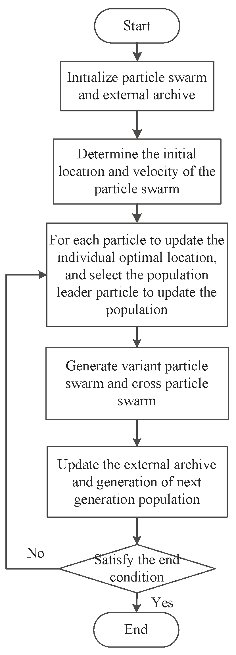
In order to solve the problem that MOPSO can easily fall into local optimization in the process of optimization, the current study introduces a mutation factor and a crossover factor derived from the genetic algorithm so that the improved MOPSO algorithm has the characteristics of fast optimization and escaping local optimization. The process for MOPSO with elite and external archiving strategies is as follows and the flowchart is shown in Figure 4.
Step 1: Initialize particle swarm and external archive. Calculate the fitness of the current particle, and the initialized Pareto solution is placed in an external archive. The size of the external archive is usually set in advance to determine the maximum number of non−inferior solutions to be retained in the archive.
Step 2: Determine the initial location and velocity of the particle swarm. Assuming that population   P t has M particles in λ generations, each particle   β has a location vector χ β = χ 1 β , χ 2 β , , χ M β and a velocity vector ν β = ν 1 β , ν 2 β , , ν M β . When generating the population   λ + 1 , each particle β updates the location and velocity according to Formula (10):
ν j , λ + 1 β = w ν j , λ β + c 1 R 1 P j , λ β + χ j , λ β + c 2 R 2 P j , λ β , g + χ j , λ β , χ j , λ + 1 β = χ j , λ β + ν j , λ + 1 β
where   j = 1 , 2 , , M ;   w is inertia weight; C 1 and C 2 are positive constants; R 1 and R 2   are random numbers between 0 , 1 and P j , λ β , g j = 1 , 2 , , M is the best particle in the population, which guides the population to move to the optimal position.
Step 3: Update the individual optimal position for each particle, and then select the population leader particle to update the population.
In the MOPSO algorithm, the focus needs to be on how to select and update the population−leading particles to enhance the convergence and generate new particles to increase population diversity. Therefore, it is necessary to find a global best particle as the leading particle from the Pareto solution set. Man−Fai Leung proposed a new leading particle selection algorithm [25]. In this algorithm, the particle is free to choose its own leader by a square root distance calculation. The square root distance between two particles   β 1 and β 2   is calculated as follows:
S R D β 1 , β 2 = i = 1 m f i χ β 1 f i χ β 2
where f i (x) is the optimization objective function.
In each generation, calculate the square root distance between each particle in the population and all the external archived particles. The external archived particle with the shortest square root distance is selected as the leader of the particle, that is:
M i n ( i = 1 m f i y 1 f i β , , i = 1 m f i y η f i β      
where m is the number of objective functions and y 1 , y 2 , , y n is an archive set with η members.
Step 4: Generate the variant−particle swarm and crossover−particle swarm. Firstly, use roulette to select m 1   particles from the previous generation and put them in the pool M i   to be operated, and set the crossover probability   p c   and mutation probability   p m . Secondly, one particle is randomly selected from M i   each time, and this particle is mutated according to the randomly generated mutation point, the number of the variant particles is   m 1 × p m . Thirdly, two particles are randomly selected from M i   each time, and the two particles are crossed according to the randomly generated intersection point; the number of the crossed particle is   m 1 × p c . Finally, the variant−particle swarm and the crossover−particle swarm are combined with the updated particle population in step 3.
Step 5: Update the external archive and retain the first M particles as the next generation population according to the non−inferior hierarchical sorting.
Step 6: Judge the termination condition and check the number of iterations. If neither of these two conditions is met, go back to step 3.
After the iteration, the external archive is the Pareto solution set of the optimization problem. The parameters of the MOPSO are shown in Table 2.

3.2. Results and Discussion

In order to analyze whether grid size has an impact on optimization results and its application in different engineering scenarios, different grid sizes are used for simulation. In the simulation experiment, the grid of the composite material plate is 9 × 9 and 11 × 11, respectively, and then the sensor position a is 64 and 100, the impact degree a is 2, and the impact category b is 128 and 200.
After the optimization of MOPSO, the sensor network results corresponding to a different number of sensors in each grid size can be obtained. The optimization results of the 9 × 9 grid are shown in Table 3, and the optimization results of the 11 × 11 grid are shown in Table 4.
It can be seen from Table 3 and Table 4 that: (1) In one Pareto solution set, the value of the minimum distance among categories increases gradually with the increasing number of sensors, which is in line with expectations. (2) The results of sensor distribution optimization are inheritable. The sensor location with a large design threshold includes the sensor location with a small design threshold. This verifies the correctness of the optimization method. (3) With the same number of sensors, the minimum distance between categories of the second Pareto solution set is smaller than that in the first Pareto solution set. This indicates that the data of the first Pareto solution set are easier to classify by class than the data of the second Pareto solution set.
By comparing Table 3 and Table 4, it can be found that: (1) The greater the density of the divided grid, the more categories need to be identified, and the smaller the minimum difference between categories. (2) By increasing the number of sensors, the value of the minimum distance between categories can be improved. The grid size can be selected according to the different recognition rates.
This method can be applied to different engineering scenarios by changing the grid size. Under the same conditions, the smaller the grid size, the slower the optimization speed, and the smaller the differences between categories. The grid size and the number of sensors can be selected to match the actual engineering situation.

4. Method Evaluation

In order to verify the recognition effect of the optimized sensor network when the composite plate is impacted, and prove the effectiveness of the sensor distribution optimization method, an experimental system is established. According to the above analysis of different grid sizes, the result obtained from the 9 × 9 grid is taken as an example to verify the optimization method.
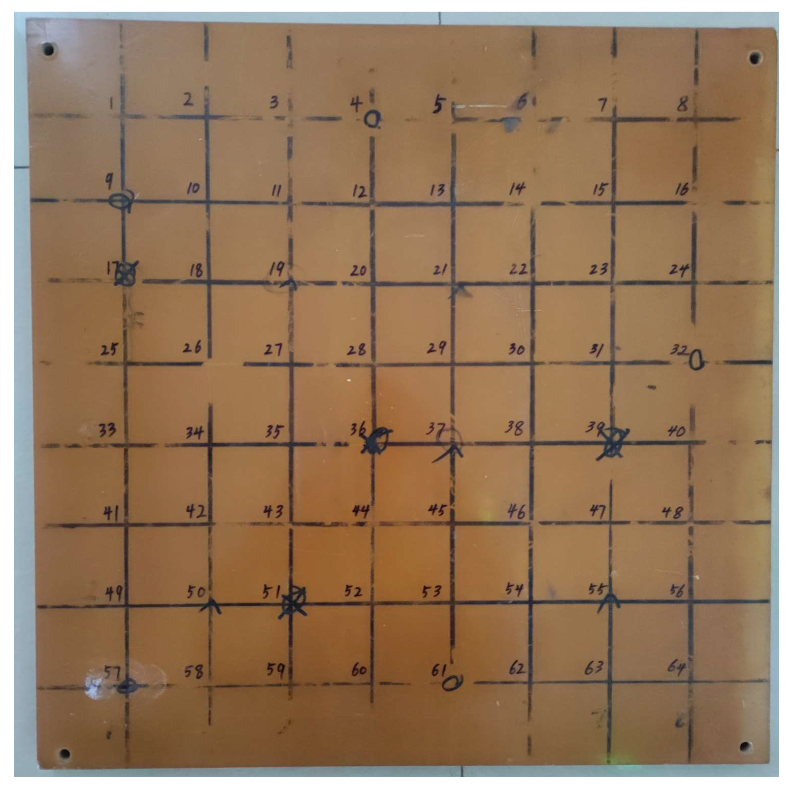
As shown in Figure 5, the composite plate is divided into a 9 × 9 grid with 64 nodes in total. A rubber ball (diameter 20 mm/mass 6.4 g) is used to impact the composite plate in freefall, and the impact is divided into full−load impact and half−load impact based on release heights of 30 cm and 15 cm, respectively. The top of each node will bear two different degrees of impact, so there are 128 impact categories in total. In addition, the underside of the 64 nodes will be used as candidate sensing points for placing sensors to obtain all kinds of impact responses.

4.1. Experimental System

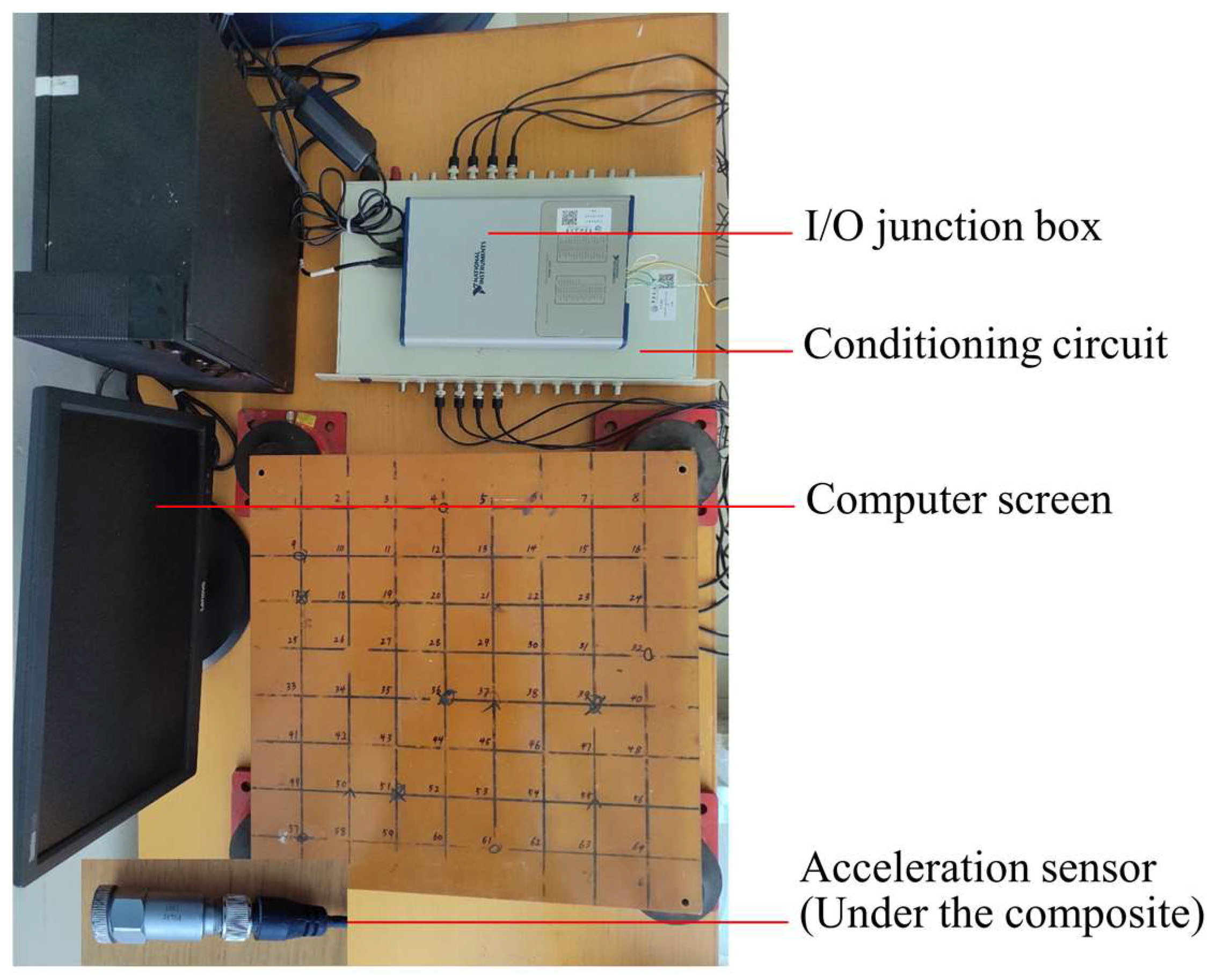
The experimental system is shown in Figure 6. The acceleration sensor collects the vibration signal from the composite board. The signal is amplified by the conditioning circuit and then imported into the data acquisition module. The parameters of the specific experimental device are shown in Table 5.

4.2. Localization Methodology

In the experiment, the signals obtained by multiple sensors were arranged in sequence and spliced into one−dimensional time−domain signals. The experiment is repeated 100 times for 128 impact categories. The experiment is carried out with the number of sensors set to two, three, and four. The following is an example of the procedure with four sensors to illustrate the effective recognition of different impact categories.
Step 1: Divide the experimental data. From the 100 samples of each impact category mentioned above, 50 samples are randomly selected as training samples, and the remaining 50 samples are used as test samples.
Step 2: Processing of training samples. Training samples in every category are judged by the Pauta criterion to eliminate the gross error, and then the remaining samples are used as the final training samples.
Step 3: Obtain the characteristic matrix of the training samples. Firstly, the AR model is used to extract the frequency−domain features of the training samples that have been spliced into one−dimensional time−domain signals. Secondly, according to the LPP method, the frequency−domain feature matrix of the training samples is reduced to obtain the training−sample feature matrix. The projection matrix used in the process is A .
Step 4: Processing of the test samples. Each test sample and all training sample sets are judged to eliminate the test samples that do not satisfy the Pauta criterion, and the remaining samples are used as the final test samples.
Step 5: Obtain the characteristic matrix of the test sample. The AR model is used to extract the frequency−domain features of the test samples that have been spliced into one-dimensional time−domain signals, and the LPP method based on the projection matrix A is used to reduce the data dimension to obtain the test−sample feature matrix.
Step 6: Impact category recognition based on probabilistic neural network (PNN). PNN has the advantages of a simple learning process, fast learning speed, and accurate classification, which incorporates the advantages of radial basis function neural network and the classical probability density estimation principle. Compared with a traditional feedforward neural network, PNN has more significant advantages in pattern classification [26]. Therefore, PNN is used as the classifier here.
In the PNN method, the test samples are the input layer and pass through the model layer composed of training samples to the summation layer, and the output layer finally outputs the classification probability f u .
  f u = 1 a 2 π δ × 4 2 σ δ × 4 q = 1 a e x p ( φ = 1 δ × 4 b τ φ u x q φ 2 2 σ 2 )    
where a is the number of training samples for each category, σ is the smoothing parameter, and the value of the smoothing parameter is 0.15, b τ φ is the τ t h   data of the φ t h neuron of each category, and x q φ represents training samples for each category.
The output layer compares the predicted probabilities of each category in the summation layer, and the maximum probability will become the predicted target category.

4.3. Experiment Result and Discussion

In order to verify the effectiveness of the optimization method, three groups of sensor distribution networks with 2, 3, and 4 sensors in the Pareto solution set are selected for impact experiments. By comparing the difference in impact recognition, different sensor networks recognition results and detailed data are obtained, as shown in Figure 7 and Table 6. The recognition rate of 128 types is shown in Figure 7. The data acquisition for the impact recognition rate calculation is completed by the system shown in Figure 6.
(1) As can be seen from Table 6, in the process of recognition, with the increasing number of sensors, the impact average recognition rate also increases. Through the analysis, it is concluded that increasing the number of sensors can provide more abundant information on impact categories, enlarge the differences between impact categories, and improve the impact recognition rate. This is consistent with the trend in the minimum distance between categories in Table 3.
(2) Combining Table 6 and Figure 7, it can be seen that, when the number of sensors in the sensor network is 2, 3, or 4, the impact recognition rates of the half−load impact categories are slightly higher than those of the full−load impact categories. Through the analysis, it is found that, due to the impact height, the realization of the full−load impact is more difficult to achieve and less stable than the half−load impact. This impact mode has more experimental errors resulting in more scattered samples of the full−load impact test data. The standard deviation is also larger than that of the half−load impact, which leads to a slight decrease in the recognition rate. However, on the whole, the results are still in line with expectations.
(3) With the increasing number of sensors, the single impact identification time gradually increases from 14.09 ms to 19.66 ms, and 21.39 ms. Therefore, it is necessary to select sensor networks according to the requirements of real−time performance and recognition rate in practical engineering applications.
In order to demonstrate the effectiveness of the proposed method, the dual objective functions I and II are defined by energy analysis of wavelet bands and principal component analysis (PCA). Based on the same simulation database and multi−objective particle swarm optimization algorithm, the sensor network is optimized, and impact monitoring experiments are carried out. Table 7 gives specific information about the two methods, and Table 8 shows the optimization results of sensor networks obtained by different methods and the corresponding impact recognition rate.
As shown in Table 8, with the increasing number of sensors, the impact recognition rates of the two methods increase in varying degrees. This indicates that effectively increasing the number of sensors can provide more information for impact monitoring. When the number of sensors is four, the average impact recognition rates of the two methods are 85.04% and 76.95%, respectively, which largely meet the requirements of impact monitoring. However, when the number of sensors is the same, the average recognition rate of method A is higher than that of method B, and the difference becomes more obvious with a decreasing number of sensors. This shows that the method of an AR model combined with LPP is better than the method of wavelet band energy analysis combined with PCA in defining the dual objective function of sensor distribution optimization and identifying 128 impact categories.

5. Conclusions

In this article, a sensor network distribution optimization method for impact monitoring of composite plates is proposed, which aims to effectively monitor the health status of composite plates with fewer sensors through the optimization of sensor distribution. The number of sensors and the minimum difference between categories are taken as objective functions I and II. Objective function II is defined by finite element analysis, the AR model, and the LPP method, and an optimization method based on the MOPSO can obtain more effective optimization results of sensor distribution. The conclusions are as follows:
(1) According to the optimization results based on the simulation data, the difference between impact categories will decrease with the increase in the number of impact categories, and the difference between impact categories will increase with the increase in the number of sensors.
(2) According to the results of the impact recognition experiment, a satisfactory recognition effect can be obtained with as few sensors as possible by optimizing sensor distribution, and the impact recognition rate of half−load impact is slightly higher than full−load impact under the same conditions. As the number of sensors increases, the recognition rate and recognition time also increase.
(3) According to a comparative study, the AR model combined with the LPP method is better than the energy analysis of wavelet bands combined with PCA method in defining the dual objective function of sensor distribution optimization.

Author Contributions

Conceptualization, P.L. and J.T.; Investigation, J.T. and Y.D.; Methodology, P.L. and Y.D.; Writing—original draft, P.H.; Writing—review & editing, G.T. and J.Z. All authors have read and agreed to the published version of the manuscript.

Funding

This research received no external funding.

Institutional Review Board Statement

Not applicable.

Informed Consent Statement

Not applicable.

Data Availability Statement

Not applicable.

Acknowledgments

The National Natural Science Foundation of China, 52165016, Damage self−repair structure of resin matrix composites based on dual−scale collaborative optimization and wallless microvascular network carriers, 2022−01 to 2025−12.; Scientific and Technological Research Project of the Education Department of Jiangxi Province, GJJ210631, Health monitoring of magnetic suspension girder under variable working conditions based on sensor distribution optimization, 2022−01 to 2023−12.

Conflicts of Interest

The authors declare no conflict of interest.

References

  1. Park, C.Y.; Kim, J.H.; Jun, S.-M.; Kim, C.-G. Localizations and force reconstruction of low-velocity impact in a composite panel using optical fiber sensors. Adv. Compos. Mater. 2012, 21, 357–369. [Google Scholar] [CrossRef]
  2. Shrestha, P.; Kim, J.-H.; Park, Y.; Kim, C.-G. Impact localization on composite wing using 1D array FBG sensor and RMS/correlation based reference database algorithm. Compos. Struct. 2015, 125, 159–169. [Google Scholar] [CrossRef]
  3. Pieczonka, L.; Aymerich, F.; Staszewski, W.J. Impact Damage Detection in Light Composite Sandwich Panels. Procedia Eng. 2014, 88, 216–221. [Google Scholar] [CrossRef]
  4. Guo, F.; Zhang, P.; Zhang, D.; Han, X.; Fei, Q. Localization of low-velocity impact by using fiber brag grating sensors based on wavelet packet energy eigenvector. J. Vib. Shock. 2017, 36, 184–189. [Google Scholar]
  5. Li, T.; Zeng, J.; Zhang, J.; Guo, X.; Xiong, Z.; Jia, H.; Liang, D. Impact localization algorithm on wing model using optical fiber sensors based on time-difference identification. J. Optoelectron. 2017, 28, 1337–1343. [Google Scholar]
  6. Gao, D. Research on structure health monitoring ultrasonic guided wave based on machine learning method. Fiber Compos. 2020, 37, 3–8. [Google Scholar]
  7. Wu, S.; Zhang, X.; Wang, L.; Huang, M. Optimal placement of sensors based on improved artificial fish swam algorithm. J. Nanchang Univ. Eng. Ed. 2019, 41, 253–259. [Google Scholar]
  8. Eberhart, R.; Kennedy, J. A New Optimizer Using Particle Swarm Theory. In Proceedings of the 1995 6th International Symposium on Micro Machine and Human Science, Nagoya, Japan, 4–6 October 1995; IEEE: Piscataway, NJ, USA. [Google Scholar]
  9. Kuang, K.S.C.; Maalej, M.; Quek, S.T. An Application of a Plastic Optical Fiber Sensor and Genetic Algorithm for Structural Health Monitoring. J. Intell. Mater. Syst. Struct. 2006, 17, 361–379. [Google Scholar] [CrossRef]
  10. Buczak, A.L.; Wang, H.; Darabi, H.; Jafari, M.A. Genetic algorithm convergence study for sensor network optimization. Inf. Sci. 2001, 133, 267–282. [Google Scholar] [CrossRef]
  11. Tong, K.; Bakhary, N.; Kueh, A.; Yassin, A.M. Optimal sensor placement for mode shapes using improved simulated annealing. Smart Struct. Syst. 2014, 13, 389–406. [Google Scholar] [CrossRef]
  12. Yi, T.-H.; Li, H.-N.; Gu, M.; Zhang, X.-D. Sensor Placement Optimization in Structural Health Monitoring Using Niching Monkey Algorithm. Int. J. Struct. Stab. Dyn. 2014, 14, 1440012. [Google Scholar] [CrossRef]
  13. Ho, J.-H.; Shih, H.-C.; Liao, B.-Y.; Chu, S.-C. A ladder diffusion algorithm using ant colony optimization for wireless sensor networks. Inf. Sci. 2012, 192, 204–212. [Google Scholar] [CrossRef]
  14. Kim, H.; Chang, S.; Kim, J. Consensus Achievement of Decentralized Sensors Using Adapted Particle Swarm Optimization Algorithm. Int. J. Distrib. Sens. Netw. 2014, 10, 1–13. [Google Scholar] [CrossRef] [Green Version]
  15. Céspedes-Mota, A.; Castañón, G.; Martínez-Herrera, A.F.; Cárdenas-Barrón, L.E. Optimization of the Distribution and Localization of Wireless Sensor Networks Based on Differential Evolution Approach. Math. Probl. Eng. 2016, 2016, 1–12. [Google Scholar] [CrossRef]
  16. Coello, C.A.C.; Reyes-Sierra, M. Multi-Objective Particle Swarm Optimizers: A Survey of the State-of-the-Art. Int. J. Comput. Intell. Res. 2006, 2, 287–308. [Google Scholar] [CrossRef]
  17. Rashmi, C.; Shashikala, T.; Neetesh, K. FZ enabled Multi-objective PSO for multicasting in IoT based Wireless Sensor Networks. Inf. Sci. 2019, 498, 1–20. [Google Scholar]
  18. Lu, H.; Xu, Y. Application research of Ballastless track health monitoring scheme based on BIM technology. J. East China Jiaotong Univ. 2022, 39, 86–93. [Google Scholar]
  19. Lu, Z.; Zhou, Y.; Li, J.; Wang, Z. Rail transit infrastructure monitoring and analysis of vibration response. J. East China Jiaotong Univ. 2021, 38, 41–46. [Google Scholar]
  20. Li, P.; Huang, L.; Peng, J. Sensor distribution optimization for structural impact monitoring based on NSGA-II and wavelet decomposition. Sensors 2018, 18, 42–64. [Google Scholar] [CrossRef] [Green Version]
  21. Al-Bugharbee, H.; Trendafilova, I. A fault diagnosis methodology for rolling element bearings based on advanced signal pretreatment and autoregressive modelling. J. Sound Vib. 2016, 369, 246–265. [Google Scholar] [CrossRef] [Green Version]
  22. Liu, T.; Zheng, M.; Chen, Z.; Zhu, J.; Hua, H. Using AR model and fractal geometry for condition monitoring of working machinery. J. Mech. Strength 2001, 23, 61–65. [Google Scholar]
  23. Akaike, H. A Bayesian analysis of the minimum AIC procedure. Ann. Inst. Stat. Math. 1978, 30, 9–14. [Google Scholar] [CrossRef]
  24. Xu, Y.; Zhong, A.; Yang, J.; Zhang, D. LPP solution schemes for use with face recognition. Pattern Recognit. 2010, 43, 4165–4176. [Google Scholar] [CrossRef]
  25. Leung, M.-F.; Ng, S.-C.; Cheung, C.-C.; Lui, A.K. A new strategy for finding good local guides in MOPSO. In Proceedings of the 2014 IEEE Congress on Evolutionary Computation (CEC), Beijing, China, 6–11 July 2014. [Google Scholar] [CrossRef]
  26. Dong, S.; Li, R. Traffic identification method based on multiple probabilistic neural network mode. Neural Comput. Appl. 2019, 31, 473–487. [Google Scholar] [CrossRef]
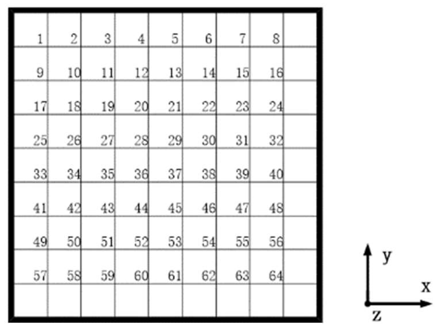
Figure 1. Division diagram with 9 × 9 grid size.
Machines 10 01154 g001
Figure 2. Finite element analysis model of the composite laminates.
Machines 10 01154 g002
Figure 3. Response of the 36th lower node under full−load impact at the 36th upper node.
Machines 10 01154 g003
Figure 4. MOPSO flowchart.
Machines 10 01154 g004
Figure 5. Grid layout on the composite plates.
Machines 10 01154 g005
Figure 6. The experimental system.
Machines 10 01154 g006
Figure 7. Impact recognition rate with different numbers of sensors.
Machines 10 01154 g007
Table 1. Parameters of composite plates.
EquipmentParameter
thickness and area15 mm × 500 mm × 500 mm
elastic modulus E Z = 7.2   GPa , E x = E y = 6.9   GPa
Poisson ratio V x z = V y z = 0.29 , V x y = 0.28
shear elasticity G x z = G y z = 7.6   GPa , G x y = 4.4   GPa
density 2100   Kg / m 3
Table 2. Parameters of the MOPSO optimization algorithm.
ParameterNumeric
individual number of initial population800
maximum inertia weight0.4
minimum inertia weight0.95
maximum value of self−learning factor2.5
maximum value of group learning factor2.5
mutation probability0.1
crossover probability0.25
Table 3. The optimization results of the 9 × 9 grid.
First Pareto Solution SetSecond Pareto Solution Set
Designed ThresholdObjective Function ISensor No.Objective
Function II
Objective
Function I
Sensor No.Objective
Function II
5510 13 29 30 420.010609665259 23 36 44 520.0106096643
411 14 37 380.00817384898411 14 20 270.00817384895
37 18 370.00540325603316 28 540.00540325602
211 210.00207577165244 540.00207577163
1593.35 × 10−111211.08 × 10−11
337 18 370.00540325603316 28 540.00540325602
211 210.00207577165244 540.00207577163
1593.35 × 10−111211.08 × 10−11
11593.35 × 10−111211.08 × 10−11
Table 4. The optimization results of the 11 × 11 grid.
First Pareto Solution SetSecond Pareto Solution Set
Designed ThresholdObjective Function ISensor No.Objective
Function II
Objective
Function I
Sensor No.Objective
Function II
5533 53 60 95 990.0042845361656 52 55 90 950.00425298431
464 67 82 890.00353586021419 37 67 890.00351594635
36 27 890.00222758237360 68 820.00222758192
234 370.00138900543282 890.00106970087
1632.3215 × 10−111961.9516 × 10−11
336 27 890.00222758237360 68 820.00222758192
234 370.00138900543282 890.00106970087
1632.3215 × 10−111961.9516 × 10−11
11632.3215 × 10−111961.9516 × 10−11
Table 5. Experimental equipment parameters.
EquipmentModel NumberParameters
acceleration sensorCA−YD−188Twith a range of −10 g to 10 g, sensitivity is 500 mV/g,
frequency response is 0.6~5000.
conditioning circuitYE3826A12−channel analog input channel, custom cable connector
kits and mounting accessories.
I/O junction boxNI−USB−635616 analog inputs at 16 bits,
1 MS/s (multichannel), 1.25 MS/s (single channel).
Table 6. Impact recognition rate of different sensor networks.
Sensor NetworkHalf Load ImpactFull Load ImpactAverage Recognition RateSingle Impact Recognition Time
(11, 21)66.25%62.19%64.22%14.09 ms
(7, 18, 37)75.86%73.59%74.73%19.66 ms
(11, 14, 37, 38)86.09%83.98%85.04%21.39 ms
Table 7. Specific information about different methods.
MethodOptimize
Database
Feature
Extraction
Data
Dimensionality
Reduction
Optimization
Algorithm for
Sensor Networks
Impact Category
Recognition
Algorithm
AANSYSARLPPMOPSOPNN
BANSYSEnergy analysis of Wavelet BandPCAMOPSOPNN
Table 8. Impact recognition rate of different methods.
Number of
Sensors
Method AMethod B
Sensor NetworkAverage
Recognition Rate
Sensor NetworkAverage
Recognition Rate
2(11,21)64.22%(28,30)25.27%
3(7,18,37)74.73%(11,25,29)59.14%
4(11,14,37,38)85.04%(27,30,50,55)76.95%
Publisher’s Note: MDPI stays neutral with regard to jurisdictional claims in published maps and institutional affiliations.