Article

Equivariant Hopf Bifurcation of a Delayed Reaction–Diffusion Predator-Prey Model with Stage Structures on a Circular Domain

1
School of Mathematical Sciences, Heilongjiang University, Harbin 150080, China
2
Engineering Research Center of Agricultural Microbiology Technology, Ministry of Education, Harbin 150080, China
3
Heilongjiang Provincial Key Laboratory of Ecological Restoration and Resource Utilization for Cold Region, Harbin 150080, China
4
Department of Mathematics, Northeast Forestry University, Harbin 150040, China
*
Author to whom correspondence should be addressed.
Axioms 2026, 15(3), 174; https://doi.org/10.3390/axioms15030174
Submission received: 13 January 2026 / Revised: 19 February 2026 / Accepted: 21 February 2026 / Published: 28 February 2026
(This article belongs to the Special Issue Nonlinear Dynamical System and Its Applications)

Abstract

This paper mainly studies the equivariant Hopf bifurcation of a delayed reaction–diffusion predator–prey model with stage structures on a two-dimensional circular domain. Firstly, we calculate the existence of steady-state solutions, and then analyze the existence of Hopf and equivariant Hopf bifurcation for the model according to bifurcation theory. Secondly, we calculate the normal form of the equivariant Hopf bifurcation. Finally, we conduct numerical simulations to verify the conclusion. And through simulation, we obtain a spatially homogeneous periodic solution, and spatially inhomogeneous periodic solution including rotating waves and standing waves on a two-dimensional circular domain, which shows rich dynamic properties on a two-dimensional space.

1. Introduction

The relationship between predators and prey is one of the important subjects in mathematical ecology because of its universality and importance. People have established various mathematical models to describe this relationship, in order to predict long-term outcomes and the impact on the entire ecosystem (see [1,2,3,4]).
Hopf bifurcation plays a fundamental role in understanding the emergence of periodic oscillations in ecological systems (see [5,6,7,8]). In predator–prey interactions, time delays arising from gestation, maturation, or resource conversion processes may destabilize an otherwise stable equilibrium and induce sustained population cycles. The occurrence of Hopf bifurcation characterizes the critical transition at which a stable steady state loses stability and a family of periodic solutions emerges. In reaction–diffusion systems, this phenomenon is further enriched by the presence of spatial effects, as temporal oscillations may interact with diffusion to generate spatially homogeneous or inhomogeneous periodic patterns (see [9,10]). Therefore, analyzing Hopf bifurcation not only provides explicit threshold conditions for stability switching with clear biological interpretations, but also helps to reveal the mechanisms underlying complex spatiotemporal dynamics in delayed predator–prey systems.
In species with distinct life stages, the juvenile and adult individuals often exhibit markedly different characteristics (see [11,12,13,14]). This is particularly evident in insect and amphibian species. They are often adapted to different environments (frequently aquatic), and have completely different dispersal characteristics. Adult insects are capable of dispersing over considerable distances, whereas their larvae are generally confined and relatively sedentary. On the other hand, for certain marine species, such as barnacles, the larvae are mobile while the adults remain sessile (see [15]). This indicates that understanding the stage structure of populations in the ecosystem is crucial for biological research. The growth and development of all species involve a dynamic process that unfolds across distinct stages. A comprehensive understanding of the different phases of a species’ life cycle, along with their unique characteristics, is essential for gaining a holistic perspective on the species from both biological and ecological standpoints (see [16]). Therefore, numerous scholars have demonstrated a profound interest in stage structure and its implications for population dynamics (see [17,18,19,20]). In [21], Pijush Panday et al. proposed the following model
d J d t = r A 1 + f α P d 1 J m J s 1 J 2 a 1 J P 1 + b 1 J , d A d t = m J d 2 A s 2 A 2 a 2 A P 1 + b 2 A + b 3 α A 2 , d P d t = e a 1 J P 1 + b 1 J + e a 2 A P 1 + b 2 A + b 3 α A 2 d 3 P ,
where J and A represents the juvenile and adult stages of the prey, respectively; P is the predator density; r is the birth rate of adult prey; s 1 and d 1 represents the intra-specific competition rate and natural mortality rate of juvenile prey, respectively; m denotes the maturation rate from juvenile to adult prey; d 2 and s 2 denotes the natural mortality rate and intra-specific competition rate of adult prey, respectively; a 1 and a 2 represents the predation rates of predators on juvenile prey and adult prey, respectively; b 1 and b 2 is the parameter scaling functional responses of juvenile and adult prey, respectively; b 3 is the strength of group defense of adult prey; e is the conversion efficiency; d 3 is the natural mortality rate of the predator; α is the anti-predator sensitivity of adult prey; f is the level of fear of the predator.
In nature, the interaction between predators and preys does not occur instantaneously, but has certain time delays. For example, the change in the number of preys does not immediately affect the change in the number of predators. When the population of prey increases, the population of predators needs time to reproduce and grow. When the population of the prey decreases, the population of the predator does not immediately decrease too, because it takes a while for them to feel the shortage of food. Therefore, to make model more realistic, many researchers have added a time delay term to the predator–prey model (see [22,23,24,25]). Similarly, for Equation (1), we introduce the digest delay τ > 0 and denote J τ = J ( t τ ) and A τ = A ( t τ ) . Then we have
d J d t = r A 1 + f α P d 1 J m J s 1 J 2 a 1 J P 1 + b 1 J , d A d t = m J d 2 A s 2 A 2 a 2 A P 1 + b 2 A + b 3 α A 2 , d P d t = e a 1 J τ P 1 + b 1 J τ + e a 2 A τ P 1 + b 2 A τ + b 3 α A τ 2 d 3 P .
Considering the uneven distribution of predators and their preys in different spacial locations within a fixed area and the trend of different species spreading to areas with lower population densities, many scholars have conducted extensive research on predator–prey models with diffusion (see [26,27,28,29,30,31,32]). The diffusion term allows the model to take into account the spatial movement of biological populations, which is crucial for understanding the dynamic behavior of populations in the real world. So, we add a diffusion factor to Equation (2) and obtain the following model:
J t = d J Δ J + r A 1 + f α P d 1 J m J s 1 J 2 a 1 J P 1 + b 1 J , A t = d A Δ A + m J d 2 A s 2 A 2 a 2 A P 1 + b 2 A + b 3 α A 2 , P t = d P Δ P + e a 1 J τ P 1 + b 1 J τ + e a 2 A τ P 1 + b 2 A τ + b 3 α A τ 2 d 3 P ,
where J = J ( t , x ) , A = A ( t , x ) and P = P ( t , x ) represent the population density of prey in the juvenile stage, adult stage and predator at location x and time t, respectively; J τ = J ( t τ , x ) , A τ = A ( t τ , x ) ; d J > 0 , d A > 0 and d P > 0 are the diffusion coefficient of prey in the juvenile stage, adult stage and predator, respectively. In this paper, we will study the equivariant Hopf bifurcation of model (3) on a two-dimensional circular domain.
We would like to mention that most of the bifurcation studies on the delayed reaction–diffusion equations are focused on the one-dimensional spatial region. In fact, it is more meaningful to study the model in (3) on a two-dimensional spatial region. The disk, as a typical region with O ( 2 ) symmetry, is used to describe many problems encountered in daily life. For example, in the field of chemistry, researchers always choose round petri dishes to observe the changes in substances. In the field of ecology, some researchers have modeled lakes as circular regions to investigate the interactions between predator and prey. Furthermore, it seems that a grassland or an island can also be simply regarded as a circular domain. Compared with the one-dimensional spatial region, the study of the bifurcation of the delayed reaction–diffusion equations on the disk is more complex. There are few studies in this area, so in this paper we investigate the equivariant Hopf bifurcation and complex spatiotemporal oscillation patterns of the model in (3) in a two-dimensional circular domain. Specifically, for a model with three equations, we derive the general expressions of the normal form coefficients A 2001 1 , A 2001 2 , provided in [33].
Letting x = r cos θ , y = r sin θ , Equation (3) with Neumann boundary conditions is transformed into polar coordinates and we obtain
J ( t , r , θ ) t = d J Δ r θ J ( t , r , θ ) + r A ( t , r , θ ) 1 + f α P ( t , r , θ ) d 1 J ( t , r , θ ) m J ( t , r , θ ) s 1 J 2 ( t , r , θ ) a 1 J ( t , r , θ ) P ( t , r , θ ) 1 + b 1 J ( t , r , θ ) , ( r , θ ) Ω , t > 0 A ( t , r , θ ) t = d A Δ r θ A ( t , r , θ ) + m J ( t , r , θ ) d 2 A ( t , r , θ ) s 2 A 2 ( t , r , θ ) a 2 A ( t , r , θ ) P ( t , r , θ ) 1 + b 2 A ( t , r , θ ) + b 3 α A 2 ( t , r , θ ) , ( r , θ ) Ω , t > 0 P ( t , r , θ ) t = d P Δ r θ P ( t , r , θ ) + e a 1 J ( t τ , r , θ ) P ( t , r , θ ) 1 + b 1 J ( t τ , r , θ ) + e a 2 A ( t τ , r , θ ) P ( t , r , θ ) 1 + b 2 A ( t τ , r , θ ) + b 3 α A 2 ( t τ , r , θ ) d 3 P ( t , r , θ ) , ( r , θ ) Ω , t > 0 J ( t , R , θ ) r = A ( t , R , θ ) r = P ( t , R , θ ) r = 0 , t 0 , 0 θ < 2 π , J ( r , t , θ ) = φ 1 ( r , t , θ ) , A ( r , t , θ ) = φ 2 ( r , t , θ ) , P ( r , t , θ ) = φ 3 ( r , t , θ ) , for ( r , θ ) Ω , t [ τ , 0 ] ,
where φ 1 , φ 2 and φ 3 are non-negative functions and Ω is a bounded disk defined as follows
Ω = ( r , θ ) : 0 r R , 0 θ < 2 π
Furthermore, the system is defined on a disk with homogeneous Neumann boundary condition. This boundary condition ensures that there is neither fluxing out of the boundary nor influx from the outside, thereby confining the population density within the disk.
The rest of this paper is organized as follows: In Section 2, we introduce the existence of steady-state solutions and bifurcation analysis. In Section 3, we calculate the normal form of the equivariant Hopf bifurcation. In Section 4, we verify the conclusion through numerical simulation.

2. Stability and Bifurcation Analysis

In this section, we mainly study the existence of steady-state solutions and the existence of Hopf bifurcation and equivariant Hopf bifurcation.
First, we prove that the solutions of the system are positive. Let
F 1 ( J , A , P ) = r A 1 + f α P d 1 J m J s 1 J 2 a 1 J P 1 + b 1 J , F 2 ( J , A , P ) = m J d 2 A s 2 A 2 a 2 A P 1 + b 2 A + b 3 α A 2 , F 3 ( J , A , P ) = e a 1 J P 1 + b 1 J + e a 2 A P 1 + b 2 A + b 3 α A 2 d 3 P .
It can be observed that, when J 0 , A 0 , and P 0 , the following results hold:
F 1 A 0 , F 1 P 0 , F 2 J 0 , F 2 P 0 , F 3 J 0 , F 3 A 0 .
We define ( J ̲ ( r , t , θ ) , A ̲ ( r , t , θ ) , P ̲ ( r , t , θ ) ) = ( 0 , 0 , 0 ) and ( J ¯ ( r , t , θ ) , A ¯ ( r , t , θ ) , P ¯ ( r , t , θ ) ) = ( J * ( t ) , A * ( t ) , P * ( t ) ) , where ( J * ( t ) , A * ( t ) , P * ( t ) ) is the unique solution of the following ordinary differential equation:
d J d t = r A d 1 J m J s 1 J 2 , d A d t = m J d 2 A s 2 A 2 , d P d t = e a 1 J P 1 + b 1 J + e a 2 A P 1 + b 2 A + b 3 α A 2 d 3 P , J ( 0 ) = φ 1 * , A ( 0 ) = φ 2 * , P ( 0 ) = φ 3 * .
where φ i * = m a x { φ i ( r , t , θ ) ( r , θ ) Ω , t [ τ , 0 ) } .
From the above analysis, the following inequality can be derived:
J ¯ t d J Δ J ¯ F 1 ( J ¯ , A ¯ , P ̲ ) 0 = 0 J ̲ t d J Δ J ̲ F 1 ( J ̲ , A ̲ , P ¯ ) , A ¯ t d A Δ A ¯ F 2 ( J ¯ , A ¯ , P ̲ ) 0 = 0 A ̲ t d A Δ A ̲ F 2 ( J ̲ , A ̲ , P ¯ ) , P ¯ t d P Δ P ¯ F 3 ( J ¯ , A ¯ , P ¯ ) 0 = 0 P ̲ t d P Δ P ̲ F 3 ( J ̲ , A ̲ , P ̲ ) , 0 φ i ( r , t , θ ) φ i * , ( r , θ ) Ω , t [ τ , 0 ) .
It follows that ( 0 , 0 , 0 ) and ( J * ( t ) , A * ( t ) , P * ( t ) ) form a pair of lower and upper solutions, so that the solution of system (4) satisfies the following inequality:
0 J ( r , t , θ ) J * ( t ) , 0 A ( r , t , θ ) A * ( t ) , 0 P ( r , t , θ ) P * ( t ) .
Applying the strong maximum principle for parabolic equations, we further obtain
J ( r , t , θ ) > 0 , A ( r , t , θ ) > 0 , P ( r , t , θ ) > 0 ( r , θ ) Ω , t 0 .
For system (4), the constant steady-state solution satisfies the following equation:
r A 1 + f α P d 1 J m J s 1 J 2 a 1 J P 1 + b 1 J = 0 , m J d 2 A s 2 A 2 a 2 A P 1 + b 2 A + b 3 α A 2 = 0 , e a 1 J P 1 + b 1 J + e a 2 A P 1 + b 2 A + b 3 α A 2 d 3 P = 0 .
Clearly, system (4) always has a zero steady-state solution, E 0 = ( 0 , 0 , 0 ) . Moreover, system (4) only has one other boundary steady-state solution in the form of E 1 = ( J 1 , A 1 , 0 ) , where ( J 1 , A 1 ) satisfies
r A d 1 J m J s 1 J 2 = 0 , m J d 2 A s 2 A 2 = 0 .
From the second equation of (6), we have J 1 = S 2 A 1 2 + d 2 A 1 m . Substituting it into the first equation of (6), we can obtain a A 1 3 + b A 1 2 + c A 1 + d = 0 , where a = s 1 s 2 2 , b = 2 s 1 s 2 d 2 , c = s 1 d 2 2 + s 2 m 2 + s 2 d 1 m , d = m 2 d 2 + d 1 d 2 m r m 2 . Therefore, if m ( r d 2 ) > d 1 d 2 , system (4) has at least one boundary steady-state solution in the form of E 1 = ( J 1 , A 1 , 0 ) .
Next, we analyze the existence of the positive steady-state solution E * = ( J * , A * , P * ) . From the third equation of (5), we have
J = d 3 ( 1 + b 2 A + b 3 α A 2 ) e a 2 A ( e a 1 b 1 d 3 ) ( 1 + b 2 A + b 3 α A 2 ) + b 1 e a 2 A : = J 0 ( A ) .
Substituting the expression of J = J 0 ( A ) into the second equation of (5), we can obtain
P = 1 + b 2 A + b 3 α A 2 a 2 A m d 3 ( 1 + b 2 A + b 3 α A 2 ) e a 2 A ( e a 1 b 1 d 3 ) ( 1 + b 2 A + b 3 α A 2 ) + b 1 e a 2 A d 2 A s 2 A 2 : = P 0 ( A ) .
Then, from the first equation of (5), one has
G ( A ) : = r A 1 + f α P 0 ( A ) d 1 J 0 ( A ) m J 0 ( A ) s 1 J 0 2 ( A ) a 1 J 0 ( A ) P 0 ( A ) 1 + b 1 J 0 ( A ) = 0 .
Obviously, G ( A ) is a rational function. After calculation, the zero-point problem of G ( A ) is equivalent to a zero-point problem of a 16-degree polynomial function. Because the coefficients of the polynomial function are too complex, we omit it here. Suppose that
( H 0 ) : G ( A ) = 0 has a positive root A * such that J 0 ( A * ) > 0 and P 0 ( A * ) > 0 ,
Then, we draw the following conclusion about the existence of a non-negative steady state for system (4).
Theorem 1. 
(i) 
System (4) always has a zero steady-state solution E 0 = ( 0 , 0 , 0 ) ;
(ii) 
System (4) has at least a boundary steady-state solution E 1 = ( J 1 , A 1 , 0 ) if m ( r d 2 ) > d 1 d 2 , where ( J 1 , A 1 ) satisfies (6);
(iii) 
System (4) has a positive steady-state solution E * = ( J * , A * , P * ) if ( H 0 ) holds, where A * is a positive root of G ( A ) = 0 , J * = J 0 ( A * ) and P * = P 0 ( A * ) .
Next, we investigate the stability of positive steady-state E * = ( J * , A * , P * ) and the existence of equivariant Hopf bifurcation. Let
f 1 = r A 1 + f α P d 1 J m J s 1 J 2 a 1 J P 1 + b 1 J , f 2 = m J d 2 A s 2 A 2 a 2 A P 1 + b 2 A + b 3 α A 2 , f 3 = e a 1 J τ P 1 + b 1 J τ + e a 2 A τ P 1 + b 2 A τ + b 3 α A τ 2 d 3 P ,
and F = ( f 1 , f 2 , f 3 ) T . Denote U ( t , r , θ ) = ( J ( t , r , θ ) , A ( t , r , θ ) , P ( t , r , θ ) ) T ; then, the linearized system of Equation (4) at E * is given by
U ( t , r , θ ) t = D r θ U ( t , r , θ ) + A U ( t , r , θ ) + B U ( t τ , r , θ ) ,
where D = d i a g ( d J , d A , d P ) , and
A = F U | ( J * , A * , P * ) = a 11 a 12 a 13 a 21 a 22 a 23 0 0 a 33 , B = F U τ | ( J * , A * , P * ) = 0 0 0 0 0 0 b 31 b 32 0 ,
with
a 11 = d 1 m 2 s 1 J * a 1 P * ( 1 + b 1 J * ) 2 , a 12 = r 1 + f α P * , a 13 = r A * f α ( 1 + f α P * ) 2 a 1 J * 1 + b 1 J * , a 21 = m , a 22 = d 2 2 s 2 A * a 2 P * ( 1 b 3 α A * 2 ) ( 1 + b 2 A * + b 3 α A * 2 ) 2 ,
a 23 = a 2 A * 1 + b 2 A * + b 3 α A * 2 , a 33 = e a 1 J * 1 + b 1 J * + e a 2 A * 1 + b 2 A * + b 3 α A * 2 d 3 , b 31 = e a 1 P * ( 1 + b 1 J * ) 2 , b 32 = e a 2 P * ( 1 b 3 α A * 2 ) ( 1 + b 2 A * + b 3 α A * 2 ) 2 .
From [32], the characteristic equation of system (7) at the positive steady-state solution E * on the disk is
Δ 0 m ( γ ) = γ 3 + M 0 m γ 2 + N 0 m γ + E 0 m + ( F 0 m γ + Q 0 m ) e γ τ = 0 , m N 0 , Δ n m ( γ ) = ( γ 3 + M n m γ 2 + N n m γ + E n m + ( F n m γ + Q n m ) e γ τ ) 2 = 0 , m N , n N ,
where N = { 1 , 2 , } , N 0 = { 0 } N ,
M n m = ( d J + d A + d P ) λ n m ( a 11 + a 22 + a 33 ) , N n m = ( d J d A + d J d P + d A d P ) λ n m 2 [ ( a 22 + a 33 ) d J + ( a 11 + a 33 ) d A + ( a 11 + a 22 ) d P ] λ n m + a 11 a 22 + a 11 a 33 + a 22 a 33 a 12 a 21 , E n m = d J d A d P λ n m 3 ( a 11 d A d P + a 22 d J d P + a 33 d J d A ) λ n m 2 + ( a 11 a 22 d P + a 11 a 33 d A + a 22 a 33 d J a 12 a 21 d P ) λ n m + a 33 ( a 12 a 21 a 11 a 22 ) , F n m = a 13 b 31 a 23 b 32 , Q n m = ( a 13 b 31 d A a 23 b 32 d J ) λ n m + b 31 ( a 13 a 22 a 12 a 23 ) + b 32 ( a 11 a 23 a 13 a 21 ) ,
λ n m = ( α n m R ) 2 and α n m is the root of the derivative function of the following Bessel function:
J n ( α ) = k = 0 + ( 1 ) k k ! ( n + k ) ! α 2 n + 2 k .
When τ = 0 , (8) becomes the following form,
Δ 0 m ( γ ) = γ 3 + M 0 m γ 2 + ( N 0 m + F 0 m ) γ + E 0 m + Q 0 m = 0 , m N 0 , Δ n m ( γ ) = ( γ 3 + M n m γ 2 + ( N n m + F n m ) γ + E n m + Q n m ) 2 = 0 , m N , n N .
For convenience, denote
K 1 = { ( 0 , m ) , m N 0 } , K 2 = { ( n , m ) , n N , m N } .
According to the Routh–Hurwitz criterion, we have the following theorem.
Lemma 1. 
When τ = 0 , all the roots of the characteristic equation, Equation (8), have negative real parts if ( H 0 ) and ( H 1 ) hold for any ( n , m ) K 1 K 2 , where
( H 1 ) : M n m > 0 ; M n m ( N n m + F n m ) ( E n m + Q n m ) > 0 ; ( E n m + Q n m ) [ M n m ( N n m + F n m ) ( E n m + Q n m ) ] > 0 .
Lemma 1 shows that when τ = 0 , all roots of the characteristic equation, Equation (8), have negative real parts, which means that the positive steady-state solution E * of system (4) is asymptotically stable. And when τ = 0 , characteristic Equation (8) has no root in the right half complex plane. Then, as the bifurcation parameter τ increases from zero, if there are no characteristic roots crossing the imaginary axis into the right half plane, then the characteristic equation, Equation (8), will always have no roots in the right half complex plane. That is to say, the positive steady-state solution E * of system (4) will always be asymptotically stable.
For clarity, we briefly explain assumptions ( H 1 ). The assumption essentially constitutes the Routh–Hurwitz criterion for determining the local asymptotic stability of the steady state. By imposing conditions on the coefficients of the characteristic equation, they ensure that all eigenvalues have negative real parts, thereby guaranteeing the stability of the steady state. When some of these conditions are violated, eigenvalues may cross the imaginary axis, leading to stability switching and possibly bifurcation. Therefore, these assumptions not only have clear mathematical significance but also provide the foundation for the subsequent bifurcation analysis.
Lemma 2. 
If ( H 0 ) and ( H 1 ) hold, then γ = 0 is not a root of the characteristic Equation (8) for any τ 0 .
Proof. 
Suppose γ = 0 is a root of the characteristic equation, Equation (8); then, we have E n m + Q n m = 0 , which is contradictory to ( H 1 ) . Therefore, γ = 0 is not a root of the characteristic Equation (8) for any τ 0 . □
Lemma 2 shows that as the bifurcation parameter τ increases from zero, the roots of the characteristic equation, Equation (8), cannot cross the imaginary axis into the right half plane through the origin. Next, we investigate the existence of pure imaginary roots of the characteristic equation, Equation (8). Let i ω n m be a pure imaginary root of Δ n m ( γ ) = 0 . Then, we can obtain
( i ω n m ) 3 + M n m ( i ω n m ) 2 + N n m ( i ω n m ) + E n m + ( F n m ( i ω n m ) + Q n m ) e i ω n m τ = 0 .
Separating the real and imaginary parts, we have
ω n m 3 N n m ω n m = F n m ω n m cos ω n m τ Q n m sin ω n m τ M n m ω n m 2 E n m = F n m ω n m sin ω n m τ + Q n m cos ω n m τ .
Squaring the two equations above and adding them together, we obtain
ω n m 6 + ( M n m 2 2 N n m ) ω n m 4 + ( N n m 2 2 M n m E n m F n m 2 ) ω n m 2 + E n m 2 Q n m 2 = 0 .
Let x n m = ω n m 2 ; then, the above equation is transformed into
f ( x n m ) : = x n m 3 + a n m x n m 2 + b n m x n m + c n m = 0 ,
where
a n m = M n m 2 2 N n m , b n m = N n m 2 2 M n m E n m F n m 2 , c n m = E n m 2 Q n m 2 .
Clearly,
f ( x n m ) = 3 x n m 2 + 2 a n m x n m + b n m = 0
has no real roots if 3 b n m > a n m 2 and has two real roots,
x n m ± = a n m ± a n m 2 3 b n m 3 ,
if 3 b n m < a n m 2 . The monotonicity of f ( x n m ) can be classified into the following several cases:
Case 1
: 3 b n m > a n m 2 . In this case, we have f ( x n m ) > 0 and f ( x n m ) monotonically increasing for x n m R + ;
Case 2
: b n m < 0 . In this case, we have f ( x n m ) < 0 and f ( x n m ) monotonically decreasing for x n m ( 0 , x n m + ) and f ( x n m ) > 0 and f ( x n m ) monotonically increasing for x n m ( x n m + , ) ;
Case 3
: 0 < 3 b n m < a n m 2 and a n m > 0 . In this case, we have f ( x n m ) > 0 and f ( x n m ) monotonically increasing for x n m R + ;
Case 4
: 0 < 3 b n m < a n m 2 and a n m < 0 . In this case, we have f ( x n m ) > 0 and f ( x n m ) is monotonically increasing for x n m ( 0 , x n m ) ( x n m + , ) , and f ( x n m ) < 0 and f ( x n m ) monotonically decreasing for x n m ( x n m , x n m + ) .
To clearly depict the number of positive roots of f ( x n m ) = 0 , we make the following assumptions:
(S0)
: 3 b n m > a n m 2 , c n m > 0 ; or b n m < 0 , c n m > 0 , f ( x n m + ) > 0 ; or 0 < 3 b n m < a n m 2 , a n m > 0 , c n m > 0 ; or 0 < 3 b n m < a n m 2 , a n m < 0 , c n m > 0 , f ( x n m + ) > 0 .
(S1)
: 3 b n m > a n m 2 , c n m < 0 ; or b n m < 0 , c n m < 0 ; or 0 < 3 b n m < a n m 2 , a n m > 0 , c n m < 0 ; or 0 < 3 b n m < a n m 2 , a n m < 0 , c n m < 0 , f ( x n m ) < 0 ; or 0 < 3 b n m < a n m 2 , a n m < 0 , c n m < 0 , f ( x n m + ) > 0 .
(S2)
: b n m < 0 , c n m > 0 , f ( x n m + ) < 0 ; or 0 < 3 b n m < a n m 2 , a n m < 0 , c n m > 0 , f ( x n m + ) < 0 .
(S3)
: 0 < 3 b n m < a n m 2 , a n m < 0 , c n m < 0 , f ( x n m + ) < 0 < f ( x n m ) .
Then, if ( S k ) holds, f ( x n m ) = 0 has k positive roots.
Summarizing the above situation, we can obtain the following lemma.
Lemma 3. 
If one of ( a ) ( d ) holds, then when the bifurcation parameter τ = τ n m j k , the characteristic equation, Equation (8), has a pair of pure imaginary roots ± i ω n m for ( n , m ) K 1 K 2 .
(a) 
: Δ < 0 , c n m < 0 , f ( x n m ) = 0 has one positive root;
(b) 
: Δ > 0 , b n m < 0 , if c n m 0 , then f ( x n m ) = 0 has one positive root; if c n m > 0 , f ( x n m 2 ) < 0 then f ( x n m ) = 0 has two positive roots;
(c) 
: Δ > 0 , b n m = 0 , if a n m > 0 , c n m < 0 , then f ( x n m ) = 0 has one positive root; if a n m < 0 , c n m > 0 , f ( x n m 2 ) < 0 , then f ( x n m ) = 0 has two positive roots; if a n m < 0 , c n m 0 , then f ( x n m ) = 0 has one positive root;
(d) 
: Δ > 0 , b n m > 0 , if a n m > 0 , c n m < 0 , then f ( x n m ) = 0 has one positive root; if a n m < 0 , c n m 0 , f ( x n m 2 ) < 0 , then f ( x n m ) = 0 has two positive roots; if a n m < 0 , c n m < 0 , f ( x n m 1 ) < 0 , then f ( x n m ) = 0 has one positive root; if a n m < 0 , c n m < 0 , f ( x n m 1 ) > 0 , f ( x n m 2 ) > 0 , then f ( x n m ) = 0 has one positive root; if a n m < 0 , c n m < 0 , f ( x n m 1 ) > 0 , f ( x n m 2 ) < 0 , then f ( x n m ) = 0 has three positive roots.
Under the condition of ( a ) ( d ) , f ( x n m ) = 0 has positive roots x n m k , k = 1 , 2 , 3 , where ( n , m ) K 1 K 2 , ω n m k = x n m k , i ω n m k is a purely imaginary root of characteristic Equation (8). From (10), we can obtain
sin ω n m k τ = Q n m ( ( ω n m k ) 3 N n m ω n m k ) + F n m ω n m k ( M n m ( ω n m k ) 2 E n m ) ( ( ω n m k ) 3 N n m ω n m k ) 2 + ( M n m ( ω n m k ) 2 E n m ) 2 = Θ 1 , cos ω n m k τ = F n m ω n m k ( ( ω n m k ) 3 N n m ω n m k ) + Q n m ( M n m ( ω n m k ) 2 E n m ) ( ( ω n m k ) 3 N n m ω n m k ) 2 + ( M n m ( ω n m k ) 2 E n m ) 2 = Θ 2 .
It follows that
τ = τ n m j k : = 1 ω n m k ( arccos Θ 2 + 2 j π ) , for Θ 1 0 , 1 ω n m k ( arccos ( Θ 2 ) + ( 2 j + 1 ) π ) , for Θ 1 < 0 , k = 1 , 2 , 3 , j N 0 .
The above τ n m j k is the parameter value for which the characteristic equation, Equation (8), has a pair of pure imaginary roots ± i ω n m k , and it is also the parameter value at which the stability of the positive steady-state solution E * may change. To determine whether the stability of the positive steady-state solution E * has changed, it is also necessary to prove that there is a pair of complex roots that have changed from negative real parts through a pair of pure imaginary roots to positive real parts. This means that we need to verify the transversality condition, and if it is satisfied, the above τ n m j k is called a Hopf bifurcation point or equivariant Hopf bifurcation point.
Lemma 4. 
Supposing ( H 1 ) ( H 3 ) and one of ( a ) ( d ) are satisfied, let γ ( τ ) = α ( τ ) + i β ( τ ) be the root of Δ n m ( γ ) = 0 for ( m , n ) K 1 K 2 , satisfying α ( τ n m j k ) = 0 and β ( τ n m j k ) = ω n m k ; then,
R e d γ d τ | τ = τ n m j k 0 ,
and the sign of R e d γ d τ | τ = τ n m j k is the same as that of f ( x n m k ) , k = 1 , 2 , 3 .
Proof. 
Derive τ on both sides of the characteristic equation, Equation (8),
( 3 γ 2 + 2 M n m γ + N n m ) d γ d τ + F n m e γ τ d γ d τ + ( F n m γ + Q n m ) e γ τ ( τ d γ d τ γ ) = 0 .
Organize the above equation into
d γ d τ = γ e γ τ ( F n m γ + Q n m ) 3 γ 2 + 2 M n m γ + N n m + F n m e γ τ τ ( F n m γ + Q n m ) e γ τ ,
then,
d γ d τ 1 = 3 γ 2 + 2 M n m γ + N n m ( γ 4 + M n m γ 3 + N n m γ 2 + E n m γ ) + F n m F n m γ 2 + Q n m γ τ γ .
Since τ = τ n m j k , there is γ = i ω n m k , which can be substituted into the above equation to obtain
d γ d τ 1 | τ = τ n m j k = 3 ( i ω n m k ) 2 + 2 M n m ( i ω n m k ) + N n m ( ( i ω n m k ) 4 + M n m ( i ω n m k ) 3 + N n m ( i ω n m k ) 2 + E n m ( i ω n m k ) ) + F n m F n m ( i ω n m k ) 2 + Q n m ( i ω n m k ) τ n m j k i ω n m k = N n m 3 ( ω n m k ) 2 + 2 M n m ( i ω n m k ) ( N n m ( ω n m k ) 2 ( ω n m k ) 4 ) + i ( M n m ( ω n m k ) 3 E n m ω n m k ) + F n m F n m ( ω n m k ) 2 + Q n m ( i ω n m k ) τ n m j k i ω n m k .
Taking the real part of the above equation, we have
R e d γ d τ 1 | τ = τ n m j k = 1 ( N n m ( ω n m k ) 2 ( ω n m k ) 4 ) 2 + ( M n m ( ω n m k ) 3 E n m ω n m k ) 2 [ ( N n m 3 ( ω n m k ) 2 ) · ( N n m ( ω n m k ) 2 ( ω n m k ) 4 ) + 2 M n m ω n m k ( M n m ( ω n m k ) 3 E n m ω n m k ) ] + F n m 2 ( ω n m k ) 2 ( F n m ( ω n m k ) 2 ) 2 + ( Q n m ω n m k ) 2 = 3 ( ω n m k ) 4 + 2 ( M n m 2 2 N n m ) ( ω n m k ) 2 + N n m 2 2 M n m E n m F n m 2 F n m 2 ( ω n m k ) 2 + Q n m 2 = 3 x n m 2 + 2 a n m x n m + b n m F n m 2 ( ω n m k ) 2 + Q n m 2 = f ( x n m ) F n m 2 ( ω n m k ) 2 + Q n m 2 0 .
Since R e ( d γ d τ ) 1 | τ = τ n m j k and R e d γ d τ | τ = τ n m j k have the same sign, the above lemma, Lemma 4, is proved. The above lemma, Lemma 4, shows that as the bifurcation parameter τ increases from zero, and each time it passes through a bifurcation value τ = τ n m j k , the characteristic equation, Equation (8), will have a pair of conjugate complex roots of negative real parts transformed by pure imaginary roots into conjugate complex roots of positive real parts. This will result in all the roots of the characteristic equation, Equation (8), having negative real parts when the bifurcation parameter τ < τ 0 ( τ 0 is the smallest bifurcation value), and the positive steady-state solution E * is asymptotically stable. When the bifurcation parameter τ > τ 0 , the characteristic equation, Equation (8), has at least two roots with positive real parts, and the positive-state solution E * is unstable. When τ = τ n m j k , system (4) undergoes a Hopf bifurcation or an equivariant Hopf bifurcation.
Therefore, according to the above conclusion, we can obtain the following theorem.
Theorem 2. 
Supposing either ( H 1 ) ( H 3 ) and ( Y ) holds; if one of ( a ) ( d ) holds, then there exists a bifurcation parameter, τ 0 = m i n τ n m 0 k , k = 1 , 2 , 3 , such that the following apply:
(i) 
When τ [ 0 , τ 0 ) , the positive steady-state solution E * is asymptotically stable, for ( n , m ) K 1 K 2 ;
(ii) 
When τ > τ 0 , the positive steady-state solution E * is unstable, for ( n , m ) K 1 K 2 ;
(iii)  
When τ = τ 0 m j k , system (4) undergoes a Hopf bifurcation at the positive steady-state solution E * , for j N 0 , ( n , m ) K 1 , and k = 1 , 2 , 3 ;
(iv) 
When τ = τ n m j k , system (4) undergoes an equivariant Hopf bifurcation at the positive steady-state solution E * , for j N 0 , ( n , m ) K 2 , k = 1 , 2 , 3 .

3. The Normal Form

In this section, we mainly study the equivariant Hopf bifurcation by using the normal form and the center manifold theory. Therefore, we assume that system (4) undergoes an equivariant Hopf bifurcation at the positive steady-state solution E * when τ = τ n m * (where τ n m * is the critical value at which the equivariant Hopf bifurcation occurs).
Letting J ¯ ( t , r , θ ) = J ( τ t , r , θ ) J * , A ¯ ( t , r , θ ) = A ( τ t , r , θ ) A * , P ¯ ( t , r , θ ) = P ( τ t , r , θ ) P * , we drop the bar for simplicity. Then, system (4) becomes
J ( t , r , θ ) t = τ d J Δ r θ J ( t , r , θ ) + τ [ a 11 ( J ( t , r , θ ) + J * ) + a 12 ( A ( t , r , θ ) + A * ) + a 13 ( P ( t , r , θ ) + P * ) ] + τ i + j + s 2 1 i ! j ! s ! F i j s ( 1 ) ( 0 , 0 , 0 ) J i ( t , r , θ ) A j ( t , r , θ ) P s ( t , r , θ ) , A ( t , r , θ ) t = τ d A Δ r θ A ( t , r , θ ) + τ [ a 21 ( J ( t , r , θ ) + J * ) + a 22 ( A ( t , r , θ ) + A * ) + a 23 ( P ( t , r , θ ) + P * ) ] + τ i + j + s 2 1 i ! j ! s ! F i j s ( 2 ) ( 0 , 0 , 0 ) J i ( t , r , θ ) A j ( t , r , θ ) P s ( t , r , θ ) , P ( t , r , θ ) t = τ d P Δ r θ P ( t , r , θ ) + τ [ a 33 ( P ( t , r , θ ) + P * ) + b 31 ( J ( t 1 , r , θ ) + J * ) + b 32 ( A ( t 1 , r , θ ) + A * ) ] + τ i + j + s + k + l + h 2 1 i ! j ! s ! k ! l ! h ! F i j s k l h ( 3 ) ( 0 , 0 , 0 , 0 , 0 , 0 ) J i ( t , r , θ ) A j ( t , r , θ ) P s ( t , r , θ ) J k ( t 1 , r , θ ) A l ( t 1 , r , θ ) P h ( t 1 , r , θ ) ,
of which a i j , b i j , i , j = 1 , 2 , 3 were given in Section 2, and where
F i j s ( 1 ) = i + j + s F ( 1 ) J i A j P s ( 0 , 0 , 0 ) , F i j s ( 2 ) = i + j + s F ( 2 ) J i A j P s ( 0 , 0 , 0 ) , F i j s k l h ( 3 ) = i + j + s + k + l + h F ( 3 ) J i A j P s J ( t τ ) k A ( t τ ) l P ( t τ ) h ( 0 , 0 , 0 , 0 , 0 , 0 ) .
We introduce τ = τ n m * + μ , μ R ; then, the above system (11) is equivalent to
U ( t , r , θ ) t = D ( τ ) Δ r θ U ( t , r , θ ) + L ( τ ) U t ( r , θ ) + F ( U t ( r , θ ) , τ ) ,
the Taylor expansion of D ( τ n m * + μ ) , and L ( τ n m * + μ ) as follows
D ( τ n m * + μ ) = D ˜ 0 + μ D ˜ 1 + 1 2 μ 2 D ˜ 2 + , L ( τ n m * + μ ) = L ˜ 0 + μ L ˜ 1 + 1 2 μ 2 L ˜ 2 + ,
where D ˜ 0 = D ( τ n m * ) , L ˜ 0 ( · ) = L ( τ n m * ) ( · ) is a linear operator from L to X C , and L : = C ( [ τ , 0 ] , X C ) , X C = { U ( r , θ ) W 2 , 2 ( D ) : r U ( R , θ ) = 0 , θ [ 0 , 2 π ) } . Now system (12) can be equivalent to
d U ( t ) d t = D ˜ 0 Δ r θ U ( t ) + L ˜ 0 U t + F ˜ ( U t , μ ) ,
where L 0 and F ˜ are given, respectively, by
L ˜ 0 ( φ ) = ( τ n m * + μ ) a 11 φ 1 ( 0 ) + a 12 φ 2 ( 0 ) + a 13 φ 3 ( 0 ) a 21 φ 1 ( 0 ) + a 22 φ 2 ( 0 ) + a 23 φ 3 ( 0 ) a 33 φ 3 ( 0 ) + b 31 φ 1 ( 1 ) + b 32 φ 2 ( 1 ) ,
F ˜ ( φ , μ ) = ( τ n m * + μ ) i + j + s 2 1 i ! j ! s ! F i j s ( 1 ) ( 0 , 0 , 0 ) φ 1 i ( 0 ) φ 2 j ( 0 ) φ 3 s ( 0 ) i + j + s 2 1 i ! j ! s ! F i j s ( 2 ) ( 0 , 0 , 0 ) φ 1 i ( 0 ) φ 2 j ( 0 ) φ 3 s ( 0 ) i + j + s + k + l + h 2 1 i ! j ! s ! k ! l ! h ! F i j s k l h ( 3 ) ( 0 , 0 , 0 , 0 , 0 , 0 ) φ 1 i ( 0 ) φ 2 j ( 0 ) φ 3 s ( 0 ) φ 1 k ( 1 ) φ 2 l ( 1 ) φ 3 h ( 1 ) ,
and D ˜ 0 = D , U ( t ) = ( J ( t ) , A ( t ) , P ( t ) ) T , φ = ( φ 1 , φ 2 , φ 3 ) T L . Then, system (13) becomes
d U ( t ) d t = D ˜ 0 Δ r θ U ( t ) + L ˜ 0 U t .
Let A : L X C be the infinitesimal generators representing the semigroup induced by the solution of (14) and A * be the adjoint operator of A; these satisfy the following formula:
A φ ( ϑ ) = φ ( ϑ ) , ϑ [ 1 , 0 ) , τ 0 d η ( μ , ϑ ) φ ( ϑ ) , ϑ = 0 , A * ψ ( ϱ ) = ψ ( ϱ ) , ϱ ( 0 , 1 ] , τ 0 ψ ( ϱ ) d η ( μ , ϑ ) , ϱ = 0 .
In Section 2, we establish that A has a pair of repeated purely imaginary eigenvalues ± i ω n m , which are also eigenvalues of A * . Define the central subspace P and P * to be the generalized eigenspace of A and A * about Λ 0 = { ± i ω n m , ± i ω n m } , respectively. P * is the adjoint space of P. Now, we decompose the phase space L into a center subspace P C N and its complementary Q S ; the method of decomposition uses the relationship between P and P * as a basis.
Define a bilinear pairing ( · , · ) as being given by
( ψ , φ ) = 0 R 0 2 π r ψ ( 0 ) ¯ φ ( 0 ) 1 0 ξ = 0 ϑ ψ ( ξ ϑ ) ¯ d η ( τ n m * , ϑ ) φ ( ξ ) d ξ d r d θ ,
where φ P , ψ P * .
The basis of P is
Φ r θ ( ϑ ) = ( Φ r θ 1 ( ϑ ) , Φ r θ 2 ( ϑ ) ) = ( Φ 1 ( ϑ ) ϕ ^ n m c , Φ 2 ( ϑ ) ϕ ^ n m s ) ,
where
Φ r θ 1 ( ϑ ) = ( Φ 1 ( ϑ ) ϕ ^ n m c , Φ 2 ( ϑ ) ϕ ^ n m c ) = ( e i ω n m ϑ ξ ϕ ^ n m c , e i ω n m ϑ ξ ¯ ϕ ^ n m c ) , Φ r θ 2 ( ϑ ) = ( Φ 3 ( ϑ ) ϕ ^ n m s , Φ 4 ( ϑ ) ϕ ^ n m s ) = ( e i ω n m ϑ ξ ϕ ^ n m s , e i ω n m ϑ ξ ¯ ϕ ^ n m s ) ,
and the basis for its adjoint space P * is
Ψ r θ ( ϱ ) = ( Ψ r θ 1 ( ϱ ) , Ψ r θ 2 ( ϱ ) ) T = ( Ψ 1 ( ϱ ) ϕ ^ n m c , Ψ 2 ( ϱ ) ϕ ^ n m s ) T ,
where
Ψ r θ 1 ( ϱ ) = ( Ψ 1 ( ϱ ) ϕ ^ n m c , Ψ 2 ( ϱ ) ϕ ^ n m c ) T = ( q 1 e i ω n m ϱ δ ϕ ^ n m c , q ¯ 1 e i ω n m ϱ δ ¯ ϕ ^ n m c ) T , Ψ r θ 2 ( ϱ ) = ( Ψ 3 ( ϱ ) ϕ ^ n m s , Ψ 4 ( ϱ ) ϕ ^ n m s ) T = ( q 1 e i ω n m ϱ δ ϕ ^ n m s , q ¯ 1 e i ω n m ϱ δ ¯ ϕ ^ n m s ) T .
We set ξ = ( 1 , p 1 , p 2 ) T , δ = ( 1 , q 1 , q 2 ) , and we have
( γ I + λ n m D ˜ 0 A B e γ ) ξ = 0 , δ ( γ I + λ n m D ˜ 0 A B e γ ) = 0 ,
where γ = i ω n m , and γ = i ω n m is the eigenvalue of Equation (15); then,
d J λ n m a 11 + i ω n m a 12 a 13 a 21 d A λ n m a 22 + i ω n m a 23 b 31 e i ω n m b 32 e i ω n m d P λ n m a 33 + i ω n m 1 p 1 p 2 = 0 ,
and
1 q 1 q 2 d J λ n m a 11 i ω n m a 12 a 13 a 21 d A λ n m a 22 i ω n m a 23 b 31 e i ω n m b 32 e i ω n m d P λ n m a 33 i ω n m = 0 .
Via calculation, we can obtain
p 1 = a 23 d J λ n m a 11 a 23 + a 23 i ω n m + a 21 a 13 a 13 d A λ n m a 22 a 13 + a 13 i ω n m + a 12 a 23 , p 2 = d J λ n m a 11 + i ω n m a 12 p 1 a 13 , q 1 = b 32 d J λ n m b 32 a 11 b 32 i ω n m + a 12 b 31 b 31 d A λ n m b 31 a 22 b 31 i ω n m + a 21 b 32 , q 2 = d J λ n m a 11 i ω n m a 21 q 1 b 31 e i ω n m .
So we can confirm that the basis of P is
e i ω n m τ n m * ϑ ϕ ^ n m c e i ω n m τ n m * ϑ ϕ ^ n m c e i ω n m τ n m * ϑ ϕ ^ n m s e i ω n m τ n m * ϑ ϕ ^ n m s p 1 e i ω n m τ n m * ϑ ϕ ^ n m c p ¯ 1 e i ω n m τ n m * ϑ ϕ ^ n m c p 1 e i ω n m τ n m * ϑ ϕ ^ n m s p ¯ 1 e i ω n m τ n m * ϑ ϕ ^ n m s p 2 e i ω n m τ n m * ϑ ϕ ^ n m c p ¯ 2 e i ω n m τ n m * ϑ ϕ ^ n m c p 2 e i ω n m τ n m * ϑ ϕ ^ n m s p ¯ 2 e i ω n m τ n m * ϑ ϕ ^ n m s ,
and the basis of P * is
q 1 e i ω n m τ n m * ϱ ϕ ^ n m c q ¯ 1 e i ω n m τ n m * ϱ ϕ ^ n m c q 1 e i ω n m τ n m * ϱ ϕ ^ n m s q ¯ 1 e i ω n m τ n m * ϱ ϕ ^ n m s p 1 q 1 e i ω n m τ n m * ϱ ϕ ^ n m c p ¯ 1 q ¯ 1 e i ω n m τ n m * ϱ ϕ ^ n m c p 1 q 1 e i ω n m τ n m * ϱ ϕ ^ n m s p ¯ 1 q ¯ 1 e i ω n m τ n m * ϱ ϕ ^ n m s p 2 q 1 e i ω n m τ n m * ϱ ϕ ^ n m c p ¯ 2 q ¯ 1 e i ω n m τ n m * ϱ ϕ ^ n m c p 2 q 1 e i ω n m τ n m * ϱ ϕ ^ n m s p ¯ 2 q ¯ 1 e i ω n m τ n m * ϱ ϕ ^ n m s ,
where q can be obtained by ( Ψ r θ , Φ r θ ) = I , with
q = 1 + q 1 p ¯ 1 + q 2 p ¯ 2 + e i ω n m q 2 b 31 + e i ω n m q 2 b 32 p ¯ 1 .
Theorem 3. 
The normal form truncated to the third order can be reduced to
z 1 ˙ = i w n m z 1 + B 11 z 1 μ + B 2001 z 1 2 z 4 + B 1110 z 1 z 2 z 3 , z 2 ˙ = i w n m z 2 + B 11 ¯ z 2 μ + B 2001 ¯ z 3 z 2 2 + B 1110 ¯ z 1 z 2 z 4 , z 3 ˙ = i w n m z 3 + B 11 z 3 μ + B 2001 z 3 2 z 2 + B 1110 z 1 z 3 z 4 , z 4 ˙ = i w n m z 4 + B 11 ¯ z 4 μ + B 2001 ¯ z 1 z 4 2 + B 1110 ¯ z 2 z 3 z 4 .
From [32], we can establish that the coefficients of the normal form are as follows:
B 11 = 1 2 Ψ 1 ( 0 ) ¯ ( λ n m D ˜ 1 Φ 1 ( 0 ) + L ˜ 1 Φ 1 ) , B 2001 = C 2001 + 3 2 E 2001 , B 1110 = C 1110 + 3 2 E 1110 ,
where
C 2001 = 1 6 Ψ 1 ( 0 ) ¯ A 2001 M 22 , C 1110 = 1 6 Ψ 1 ( 0 ) ¯ A 1110 M 22 , E 2001 = 1 6 Ψ 1 ( 0 ) ¯ k = 0 M 0 k c s c S y z 1 ( h 0 k 1001 c c s ) + k = 1 M 2 n k s s c S y z 4 ( h 2 n k 2000 c s s ) , E 1110 = 1 6 Ψ 1 ( 0 ) ¯ k = 0 M 0 k c s c ( S y z 1 ( h 0 k 0110 c c s ) + S y z 2 ( h 0 k 1010 c c s ) ) + k = 1 M 2 n k s s c S y z 3 ( h 2 n k 1100 c s s ) ,
with
M 22 = 0 R 0 2 π r ( ϕ ^ n m c ) 2 ( ϕ ^ n m s ) 2 d θ d r , M 0 k c s c = 0 R 0 2 π r ϕ ^ j k ϕ ^ n m c ϕ ^ n m s d θ d r , M 2 n k s s c = 0 R 0 2 π r ϕ ^ 2 n k ϕ ^ n m s ϕ ^ n m s d θ d r ,
and
h 0 k 1001 c c s ( γ ) = M 0 k c s c [ λ 0 k D ˜ 0 + L ˜ 0 ( I d ) ] 1 A 1001 , k = 0 , 1 , 2 , h 0 k 0110 c c s ( γ ) = M 0 k c s c [ λ 0 k D ˜ 0 + L ˜ 0 ( I d ) ] 1 A 0110 , k = 0 , 1 , 2 , h 0 k 1010 c c s ( γ ) = M 0 k c s c e 2 i ω γ [ 2 i ω λ 0 k D ˜ 0 + L ˜ 0 ( e 2 i ω · I d ) ] 1 A 1010 , k = 0 , 1 , 2 , h 2 n k 2000 c s s ( γ ) = M 2 n k s s c e 2 i ω γ [ 2 i ω λ 2 n k D ˜ 0 + L ˜ 0 ( e 2 i ω · I d ) ] 1 A 2000 , k = 1 , 2 , h 2 n k 1100 c s s ( γ ) = M 2 n k s s c [ λ 2 n k D ˜ 0 + L ˜ 0 ( I d ) ] 1 A 1100 , k = 1 , 2 .
To calculate the coefficients of the normal form, we also need to calculate the following values: Φ 1 ( 0 ) , Ψ 1 ( 0 ) , A 1001 , A 2000 , A 0110 , A 1010 , A 1100 , A 2001 , A 1110 and S y z k for k = 1 , 2 , 3 , 4 . From the previous calculation, we know that
Φ 1 ( 0 ) = ξ = ( 1 , p 1 , p 2 ) T , Ψ 1 ( 0 ) = q 1 δ = 1 q ( 1 , q 1 , q 2 ) .
In order to facilitate the next equations, we let ω ˜ = ω n m and τ ˜ = τ n m * ; then,
A 2000 = 2 τ ˜ A 2000 1 A 2000 2 A 2000 3 , A 1010 = 2 τ ˜ A 1010 1 A 1010 2 A 1010 3 ,
A 1100 = 2 τ ˜ A 1100 1 A 1100 2 A 1100 3 = A 1001 = A 0110 ¯ ,
A 2001 = 2 τ ˜ A 2001 1 A 2001 2 A 2001 3 , A 1110 = 2 τ ˜ A 1110 1 A 1010 2 A 1110 3 ,
where
A 2000 1 = 2 s 1 a 1 p 2 r f α p 1 p 2 , A 2000 2 = 2 s 2 p 1 2 a 2 p 1 p 2 , A 2000 3 = e a 1 p 2 e i ω ˜ τ ˜ + e a 2 p 1 p 2 e i ω ˜ τ ˜ , A 1100 1 = 4 s 1 a 1 ( p 2 + p ¯ 2 ) r f α ( p 1 p ¯ 2 + p ¯ 1 p 2 ) , A 1100 2 = 4 s 2 p 1 p ¯ 1 a 2 ( p 1 p ¯ 2 + p ¯ 1 p 2 ) , A 1100 3 = e a 1 ( p 2 e i ω ˜ τ ˜ + p ¯ 2 e i ω ˜ τ ˜ ) + e a 2 ( p 1 p ¯ 2 e i ω ˜ τ ˜ + p ¯ 1 p 2 e i ω ˜ τ ˜ ) , A 1010 1 = 4 s 1 2 a 1 p 2 2 r f α p 1 p 2 , A 1010 2 = 4 s 2 p 1 2 2 a 2 p 1 p 2 , A 1010 3 = 2 e a 1 p 2 e i ω ˜ τ ˜ + 2 e a 2 p 1 p 2 e i ω ˜ τ ˜ , A 2001 1 = 2 a 1 b 1 ( p ¯ 2 + 2 p 2 ) + 2 r f 2 α 2 ( p ¯ 1 p 2 2 + 2 p 1 p 2 p ¯ 2 ) , A 2001 2 = 2 a 2 b 2 ( p 1 2 p ¯ 2 + 2 p 1 p ¯ 1 p 2 ) , A 2001 3 = 2 e a 1 b 1 ( p ¯ 2 e 2 i ω ˜ τ ˜ + 2 p 2 ) 2 e a 2 b 2 ( 2 p 1 p ¯ 1 p 2 + p ¯ 2 p 1 2 e 2 i ω ˜ τ ˜ ) , A 1110 1 = 4 a 1 b 1 ( 2 p 2 + p ¯ 2 ) + 4 r f 2 α 2 ( p ¯ 1 p 2 2 + 2 p 1 p 2 p ¯ 2 ) , A 1110 2 = 4 a 2 b 2 ( p 1 2 p ¯ 2 + 2 p 1 p ¯ 1 p 2 ) , A 1110 3 = 2 e a 1 b 1 ( 4 p 2 + 2 p ¯ 2 e 2 i ω ˜ τ ˜ ) 2 e a 2 b 2 ( 4 p 1 p ¯ 1 p 2 + 2 p ¯ 2 p 1 2 e 2 i ω ˜ τ ˜ ) .
See Appendix A.1 for the specific calculation process. Moreover,
S y z 1 = S y z 3 = 4 s 1 a 1 p 2 r f α p 2 a 1 r f α p 1 0 4 s 2 p 1 a 2 p 2 a 2 p 1 e a 1 p 2 e a 2 p 2 e a 1 e i ω ˜ τ ˜ + e a 2 p 1 e i ω ˜ τ ˜ , S y z 2 = S y z 4 = 4 s 1 a 1 p ¯ 2 r f α p ¯ 2 a 1 r f α p ¯ 1 0 4 s 2 p ¯ 1 a 2 p ¯ 2 a 2 p ¯ 1 e a 1 p ¯ 2 e a 2 p ¯ 2 e a 1 e i ω ˜ τ ˜ + e a 2 p ¯ 1 e i ω ˜ τ ˜ .
Similarly to the above, see Appendix A.2 for detailed calculations.
Finally, substituting the above results into the expressions of B 11 , B 2001 , and B 1110 , we can obtain the values of the coefficients of the normal form.
Introducing double sets of polar coordinates,
z 1 = ρ 1 e i χ 1 , z 4 = ρ 1 e i χ 1 , z 3 = ρ 2 e i χ 2 , z 2 = ρ 2 e i χ 2 ,
we have
ρ ˙ 1 = ( a 1 μ + a 2 ρ 1 2 + a 3 ρ 2 2 ) ρ 1 , χ ˙ 1 = ω λ ^ , ρ ˙ 2 = ( a 1 μ + a 2 ρ 2 2 + a 3 ρ 1 2 ) ρ 2 , χ ˙ 2 = ω λ ^ ,
with
a 1 = R e { B 11 } , a 2 = R e { B 2001 } , a 3 = R e { B 1110 }
According to [32], when a 1 μ < 0 (>0), we know the above system (16) has six unfoldings, which means that we can obtain the sign of a 2 , a 2 + a 3 , a 2 a 3 . We can also obtain the dynamical classifications of the above system, system (16). In the next section, we will run simulations with specific data to verify our conclusions.

4. Numerical Simulations

In this section, we carry out some simulations to verify our theoretical results. Firstly, let
R = 10 , r = 7 , d 1 = 0.3 , s 1 = 0.1 , d 2 = 0.2 , s 2 = 0.1 , a 1 = 0.2 , a 2 = 1 , b 1 = 5 , b 2 = 2 , b 3 = 1 , e = 0.6 , d 3 = 0.1 , α = 2 , f = 2 , m = 0.05 , d J = 0.3 , d A = 0.3 , d P = 0.3 .
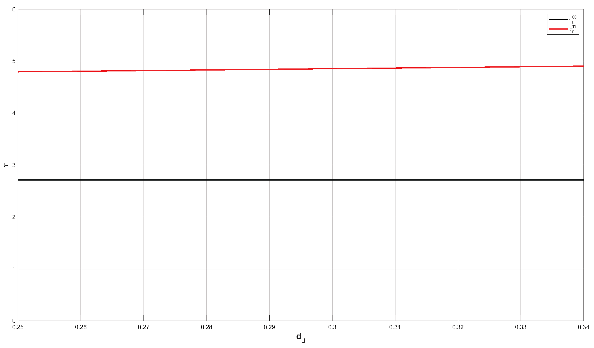
At this time, through calculation, we can conclude that E * ( 1.4258 , 0.1917 , 0.2225 ) , τ 00 0 2.7126 , τ 11 0 4.8540 .
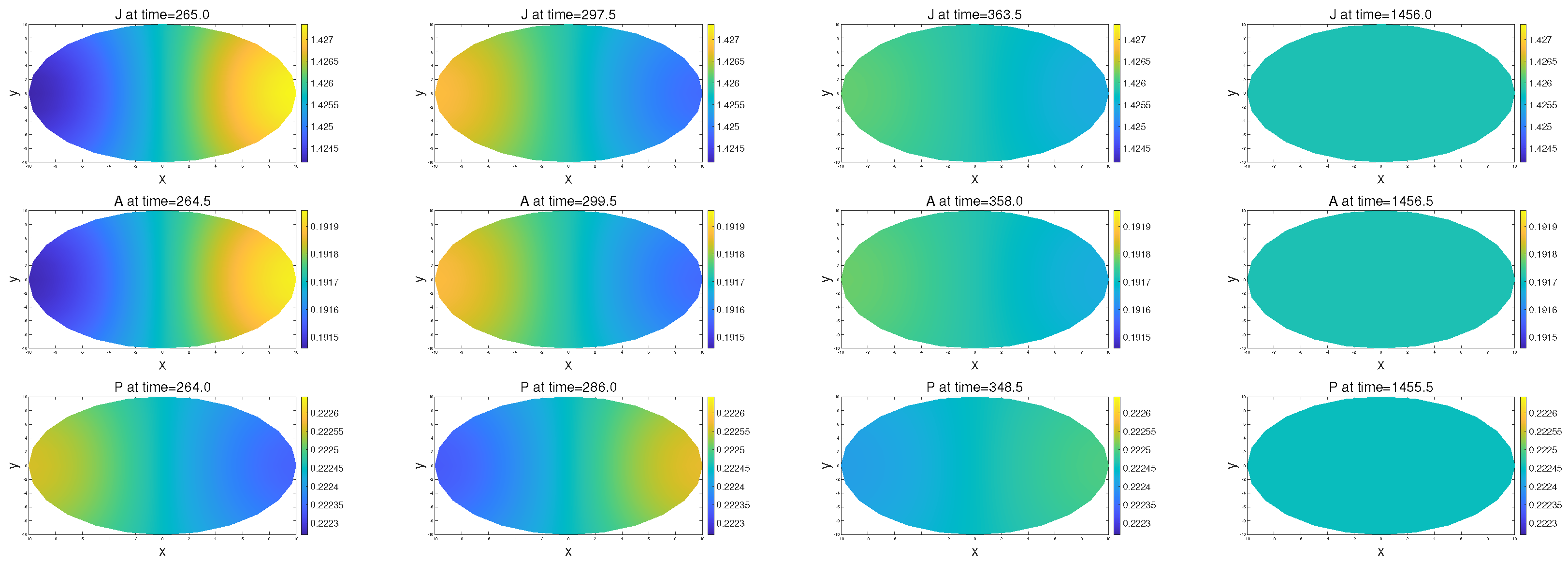
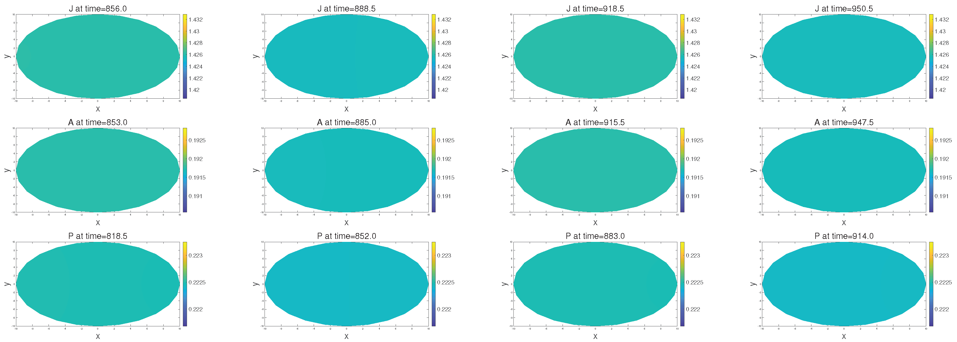
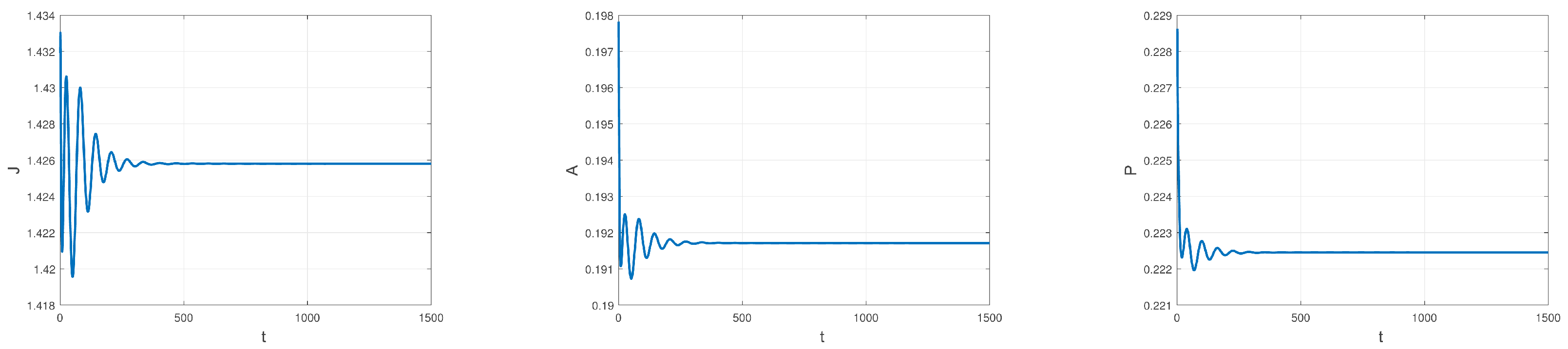
According to Theorem 2, the bifurcation generated at τ = 2.7126 is a Hopf bifurcation. We can obtain the corresponding bifurcation curves (see Figure 1). When τ [ 0 , 2.7126 ) , E * is locally asymptotically stable (see Figure 2). When τ > 2.7126 , E * is unstable and system (4) undergoes a spatially homogeneous periodic solution (see Figure 3).
In order to see if system (4) is locally asymptotically stable at the end, we take a point on the disk and draw the following graph (see Figure 4). We can see that the values of J, A, and P eventually tend to be stable as time t increases. Thus, we can confirm that system (4) is locally asymptotically stable at the steady-state solution E * .
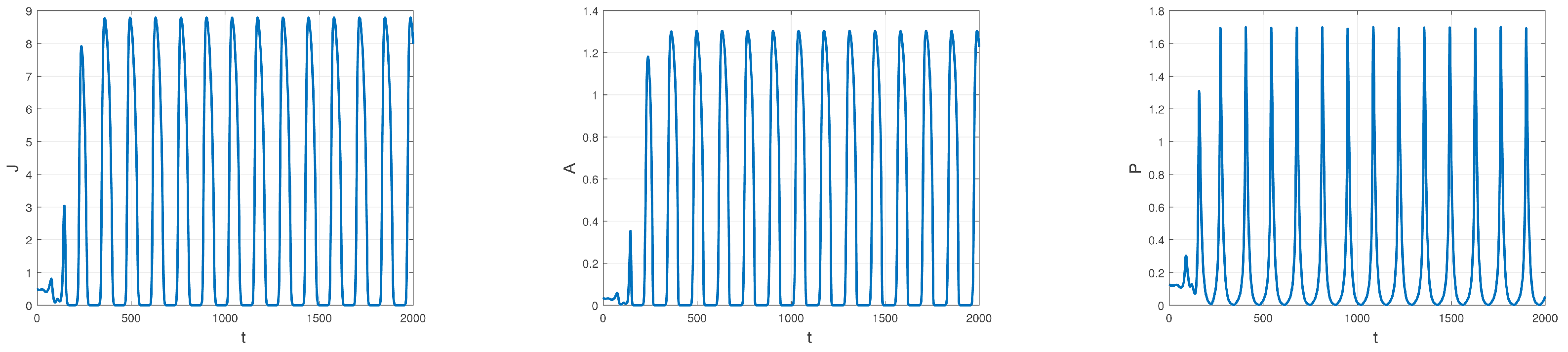
In order to see if system (4) is a spatially homogeneous periodic solution, we also draw the graph below (see Figure 5). We can see that the values of J, A, and P fluctuate periodically as time t increases. Therefore, we can confirm that system (4) undergoes a spatially homogeneous periodic solution.
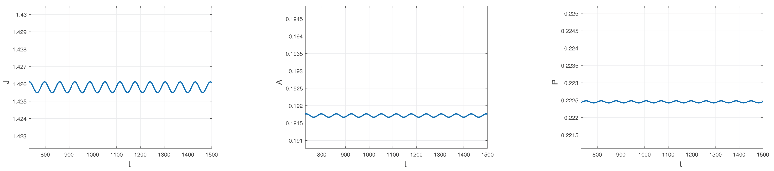
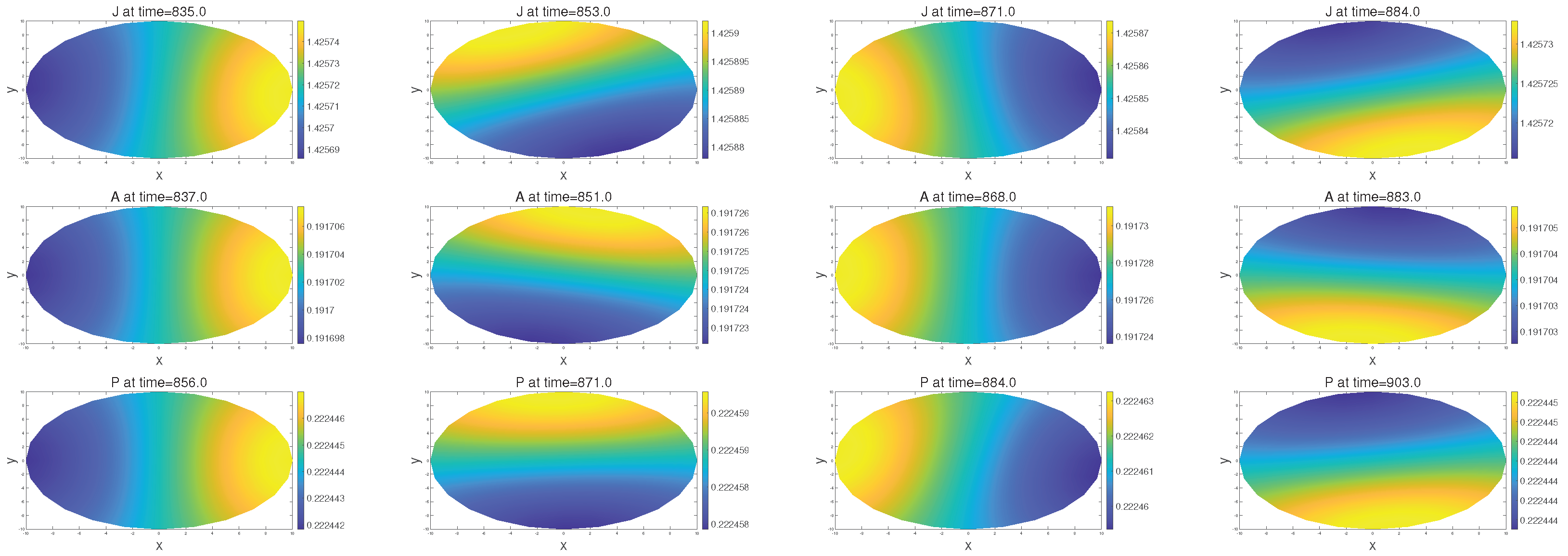
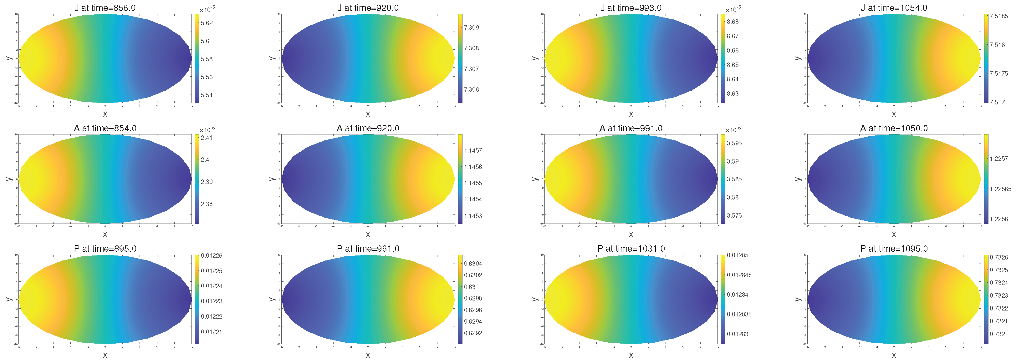
When τ = τ 11 0 4.8540 , system (4) undergoes a Hopf bifurcation. When τ < 4.8540 , E * is locally asymptotically stable. When τ > 4.8540 , E * is unstable. And the bifurcation generated at this time is an equivariant Hopf bifurcation. Let μ = 0.2540 , and through numerical simulation, we have B 11 0.0115 + 0.0437 i , B 2001 0.0011 + 0.0023 i , B 1110 0.0159 + 0.0070 i . Thus a 1 μ 0.0029 , a 2 0.0011 , a 2 + a 3 0.0170 , a 2 a 3 0.0148 . From [32], we can confirm that system (4) possesses stable rotating waves at this time (see Figure 6).
In order to verify the existence of stable rotating waves in system (4), we use the same method to plot the following diagram (see Figure 7) where we can see that the values of J, A, and P fluctuate periodically as time t increases. Thus, we can confirm that system (4) possesses stable rotating waves.
Moreover, let
R = 10 , r = 9 , d 1 = 0.3 , s 1 = 0.1 , d 2 = 0.2 , s 2 = 0.1 , a 1 = 0.2 , a 2 = 5.5 , b 1 = 6.5 , b 2 = 6 , b 3 = 6 , e = 0.6 , d 3 = 0.1 , α = 2 , f = 2 , m = 0.05 , d J = 0.3 , d A = 0.3 , d P = 0.3 .
At this time, through calculation, we can conclude taht E * ( 0.4718 , 0.0313 , 0.1201 ) , τ 12 0 8.6003 .
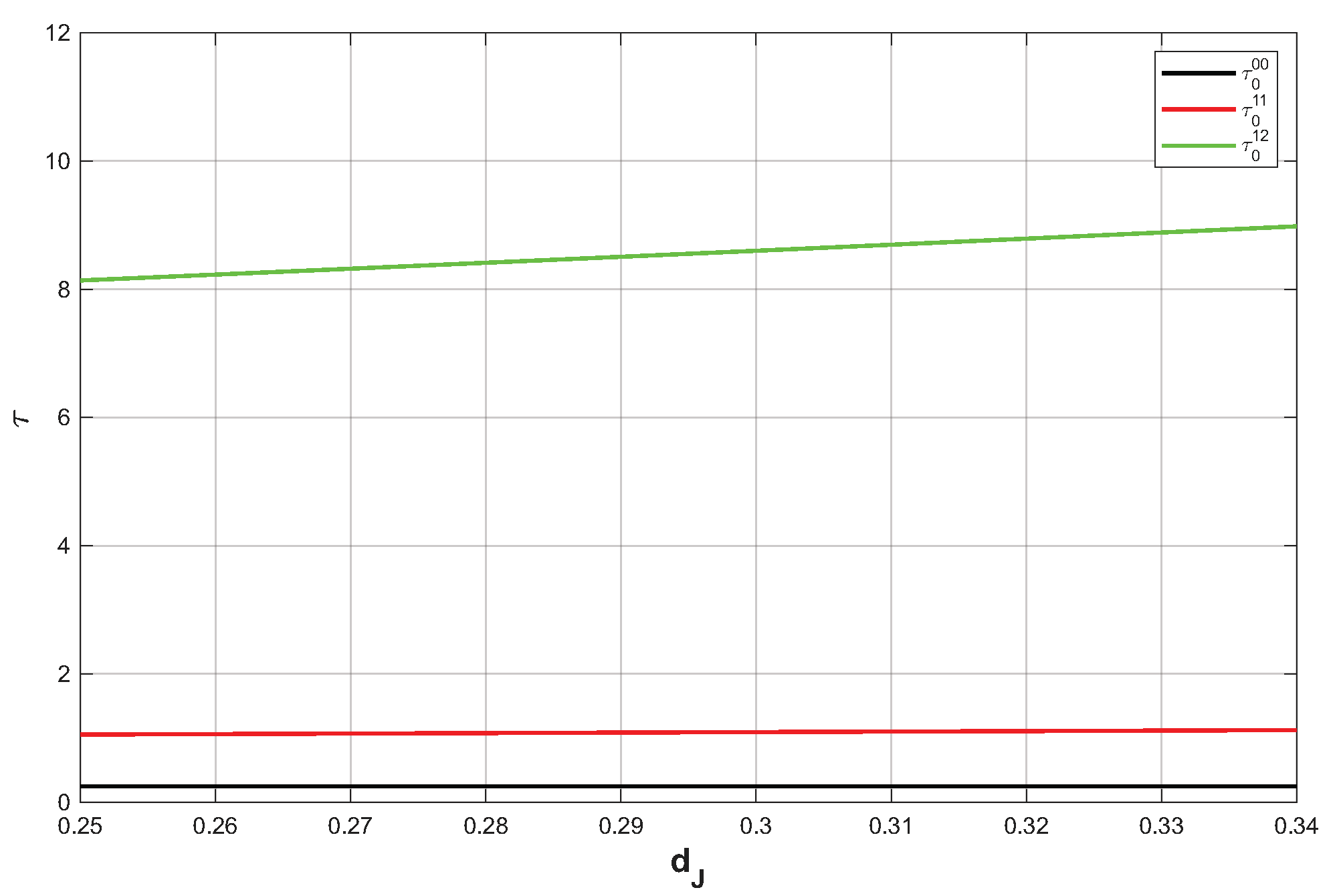
We can obtain the corresponding bifurcation; see Figure 8. When τ = τ 12 0 8.6003 , system (4) undergoes a Hopf bifurcation. When τ < 8.6003 , E * is locally asymptotically stable. When τ > 8.6003 , E * is unstable. The bifurcation generated at this time is an equivariant Hopf bifurcation. Let μ = 0.1003 ; through numerical simulation, we have B 11 0.0303 + 0.0308 i , B 2001 0.0155 + 0.0077 i , and B 1110 0.0086 + 0.0765 i . Thus a 1 μ 0.0030 , a 2 0.0155 , a 2 + a 3 0.0069 , and a 2 a 3 0.0241 . From [32], we can confirm that system (4) possesses stable standing waves at this time (see Figure 9).
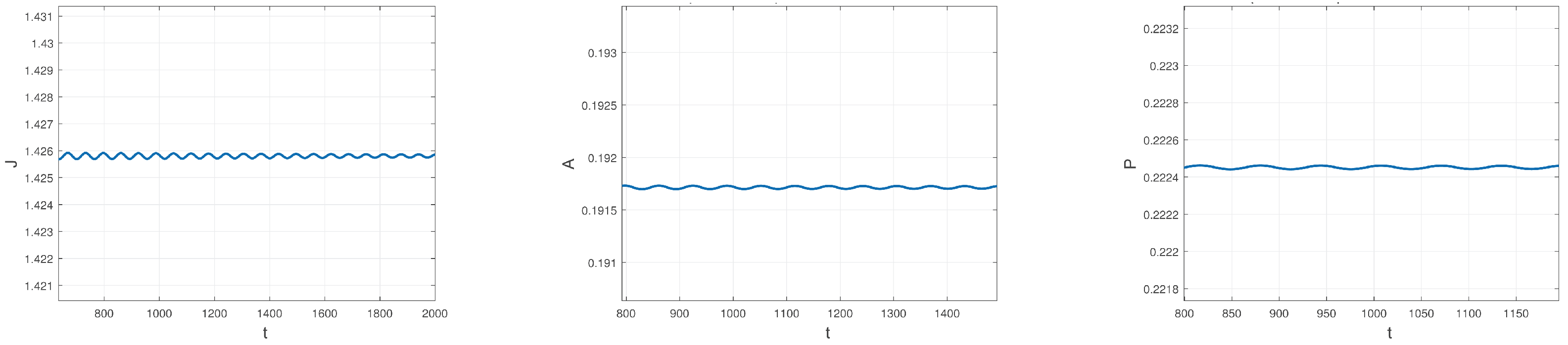
Similarly, to verify the existence of stable standing waves in system (4), we plotted the diagram below (see Figure 10), from which we can see that the values of J, A, and P fluctuate periodically as time t increases. Thus, we can confirm that system (4) possesses stable standing waves.
We tested the robustness of the observed patterns with respect to small variations in parameters along the bifurcation direction. The results show that minor changes generally do not alter the overall structure, while larger changes may significantly modify the pattern or induce new spatial structures. These observations are based on numerical simulations, and a rigorous theoretical analysis is not provided.
In the present model, the time delay parameter τ has a clear biological interpretation. It can be regarded as the gestation period of the predator population or the time required for converting consumed resources into predator biomass. The numerical simulations indicate that variations in τ can significantly influence the dynamical behavior of the system. In particular, when τ approaches certain critical values, the steady state may lose its stability. Moreover, depending on the spatial mode associated with the critical value being approached, different spatiotemporal structures may emerge accordingly. This indicates that as the gestation delay of the predator increases, the steady state of the system becomes more likely to lose its stability. Furthermore, when the delay lies within certain parameter ranges, the system may exhibit stable spatially inhomogeneous periodic solutions, such as standing waves or rotating waves.
Standing waves and rotating waves correspond to different types of spatiotemporal structures in ecological systems. A standing wave typically manifests as several relatively stable symmetry axes in space. The regions separated by these symmetry axes exhibit periodic oscillations in population density over time, and the overall spatial distribution pattern also changes periodically. This pattern reflects an ordered spatiotemporal evolution of population density under the constraint of spatial symmetry. In contrast, a rotating wave is characterized by high-density population regions that continuously rotate along the circular domain. The spatial peaks move periodically over time, while the overall structural shape remains relatively stable. From a biological perspective, a rotating wave can be interpreted as the persistent migration of the population density center in space, highlighting the combined effects of diffusion mechanisms and regional symmetry on the spatial evolution of the population distribution.

5. Conclusions

It should be noted that the normal form method is a typical local analytical tool, and its theoretical results are valid only in a neighborhood of the bifurcation point. This method constructs a center manifold near the critical parameter value and performs a low-order nonlinear expansion to derive a reduced system that describes the dynamics in the vicinity of the critical point. Therefore, normal form analysis is mainly used to characterize the dynamical properties of equilibria near the critical value, such as the emergence of periodic solutions, the direction of bifurcation, and their stability. However, when the system parameters move away from the bifurcation point, higher-order nonlinear terms may have a significant influence on the system dynamics. In such cases, the approximation provided by the normal form may no longer be valid and may fail to reveal the global dynamics of the system. Consequently, to investigate the global dynamics of the system on the disk, other analytical techniques or numerical simulations are still required.
In summary, this paper mainly investigates the local bifurcation properties of a delayed reaction–diffusion system on a disk domain and derives the conditions for the occurrence of Hopf bifurcation together with its corresponding dynamical characteristics. However, the present study is still restricted to low-codimension local analysis. Future work may further explore the possible equivariant Turing–Hopf bifurcations arising on the disk domain. Owing to the O ( 2 ) symmetry of the disk, the coupling between spatial modes and temporal oscillations may lead to more intricate bifurcation structures and dynamical behaviors. Equivariant Turing–Hopf bifurcations are typically associated with richer spatiotemporal patterns, such as rotating waves, breathing waves, and complex spatiotemporal structures induced by modal interactions. A deeper investigation of these issues would help to provide a more systematic understanding of the overall dynamical mechanisms of delayed reaction–diffusion systems on a disk.

Author Contributions

All authors participated in the writing and coordination of the manuscript. All authors have read and agreed to the published version of the manuscript.

Funding

This work is supported by the Natural Science Foundation of Heilongjiang Province (No. LH2022A002) and the National Natural Science Foundation of China (No. 12371160).

Institutional Review Board Statement

Not Applicable.

Informed Consent Statement

Not Applicable.

Data Availability Statement

Data sharing is not applicable to this article as no new data were created or analyzed in this study.

Conflicts of Interest

The authors declare no conflicts of interest. The funders had no role in the design of the study; in the collection, analyses, or interpretation of data; in the writing of the manuscript; or in the decision to publish the results.

Appendix A

Appendix A.1.  The Calculation Formula for A p ˜ 1 p ˜ 2 p ˜ 3 p ˜ 4

A 2000 = 2 τ ˜ A 2000 1 A 2000 2 A 2000 3 , A 1100 = 2 τ ˜ A 1100 1 A 1100 2 A 1100 3 , A 1010 = 2 τ ˜ A 1010 1 A 1010 2 A 1010 3 , A 2000 = A 0020 , A 1100 = A 1001 = A 0011 , A 0200 = A 0002 = A 2000 ¯ , A 0101 = A 1010 ¯ , A 0110 = A 1001 ¯ ,
A 2001 = 6 τ ˜ A 2001 1 A 2001 2 A 2001 3 , A 1110 = 6 τ ˜ A 1110 1 A 1110 2 A 1110 3 , A 2010 = 6 τ ˜ A 2010 1 A 2010 2 A 2010 3 , A 1200 ¯ = A 2100 = A 0120 = A 0021 = A 2001 = A 0201 ¯ , A 0210 ¯ = A 2010 = A 1020 ,
A 2000 1 = G 200 ( 1 ) + G 020 ( 1 ) p 1 2 + G 002 ( 1 ) p 2 2 + G 110 ( 1 ) p 1 + G 101 ( 1 ) p 2 + G 011 ( 1 ) p 1 p 2 , A 1100 1 = 2 G 200 ( 1 ) + 2 G 020 ( 1 ) p 1 p ¯ 1 + 2 G 002 ( 1 ) p 2 p ¯ 2 + G 110 ( 1 ) ( p 1 + p ¯ 1 ) + G 101 ( 1 ) ( p 2 + p ¯ 2 ) + G 011 ( 1 ) ( p ¯ 1 p 2 + p 1 p ¯ 2 ) , A 1010 1 = 2 G 200 ( 1 ) + 2 G 020 ( 1 ) p 1 2 + 2 G 002 ( 1 ) p 2 2 + 2 G 110 ( 1 ) p 1 + 2 G 101 ( 1 ) p 2 + 2 G 011 ( 1 ) p 1 p 2 , A 2000 2 = G 200 ( 2 ) + G 020 ( 2 ) p 1 2 + G 002 ( 2 ) p 2 2 + G 110 ( 2 ) p 1 + G 101 ( 2 ) p 2 + G 011 ( 2 ) p 1 p 2 , A 1100 2 = 2 G 200 ( 2 ) + 2 G 020 ( 2 ) p 1 p ¯ 1 + 2 G 002 ( 2 ) p 2 p ¯ 2 + G 110 ( 2 ) ( p 1 + p ¯ 1 ) + G 101 ( 2 ) ( p 2 + p ¯ 2 ) + G 011 ( 2 ) ( p ¯ 1 p 2 + p 1 p ¯ 2 ) , A 1010 2 = 2 G 200 ( 2 ) + 2 G 020 ( 2 ) p 1 2 + 2 G 002 ( 2 ) p 2 2 + 2 G 110 ( 2 ) p 1 + 2 G 101 ( 2 ) p 2 + 2 G 011 ( 2 ) p 1 p 2 , A 2000 3 = G 200000 ( 3 ) + G 020000 ( 3 ) p 1 2 + G 002000 ( 3 ) p 2 2 + G 110000 ( 3 ) p 1 + G 101000 ( 3 ) p 2 + G 011000 ( 3 ) p 1 p 2 + G 000200 ( 3 ) e 2 i ω ˜ τ ˜ + G 000020 ( 3 ) p 1 2 e 2 i ω ˜ τ ˜ + G 000002 ( 3 ) p 2 2 e 2 i ω ˜ τ ˜ + G 100100 ( 3 ) e i ω ˜ τ ˜ + ( G 100010 ( 3 ) + G 010100 ( 3 ) ) p 1 e i ω ˜ τ ˜ + ( G 100001 ( 3 ) + G 001100 ( 3 ) ) p 2 e i ω ˜ τ ˜ + G 000110 ( 3 ) p 1 e 2 i ω ˜ τ ˜ + ( G 010001 ( 3 ) + G 001010 ( 3 ) ) p 1 p 2 e i ω ˜ τ ˜ + G 000101 ( 3 ) p 2 e 2 i ω ˜ τ ˜ + G 000011 ( 3 ) p 1 p 2 e 2 i ω ˜ τ ˜ + G 010010 ( 3 ) p 1 2 e i ω ˜ τ ˜ + G 001001 ( 3 ) p 2 2 e i ω ˜ τ ˜ ,
A 1100 3 = 2 G 200000 ( 3 ) + 2 G 020000 ( 3 ) p 1 p ¯ 1 + 2 G 002000 ( 3 ) p 2 p ¯ 2 + G 110000 ( 3 ) ( p 1 + p ¯ 1 ) + G 101000 ( 3 ) ( p 2 + p ¯ 2 ) + 2 G 000200 ( 3 ) + 2 G 000020 ( 3 ) p 1 p ¯ 1 + 2 G 000002 ( 3 ) p 2 p ¯ 2 + G 100100 ( 3 ) ( e i ω ˜ τ ˜ + e i ω ˜ τ ˜ ) + G 100010 ( 3 ) ( p 1 e i ω ˜ τ ˜ + p ¯ 1 e i ω ˜ τ ˜ ) + G 100001 ( 3 ) ( p 2 e i ω ˜ τ ˜ + p ¯ 2 e i ω ˜ τ ˜ ) + G 000110 ( 3 ) ( p 1 + p ¯ 1 ) + G 010010 ( 3 ) ( p 1 p ¯ 1 e i ω ˜ τ ˜ + p 1 p ¯ 1 e i ω ˜ τ ˜ ) + G 010001 ( 3 ) ( p 1 p ¯ 2 e i ω ˜ τ ˜ + p ¯ 1 p 2 e i ω ˜ τ ˜ ) + G 001100 ( 3 ) ( p 2 e i ω ˜ τ ˜ + p ¯ 2 e i ω ˜ τ ˜ ) + G 001010 ( 3 ) ( p ¯ 1 p 2 e i ω ˜ τ ˜ + p 1 p ¯ 2 e i ω ˜ τ ˜ ) + G 000011 ( 3 ) ( p 1 p ¯ 2 + p ¯ 1 p 2 ) + G 001001 ( 3 ) ( p ¯ 2 p 2 e i ω ˜ τ ˜ + p 2 p ¯ 2 e i ω ˜ τ ˜ ) + G 010100 ( 3 ) ( p 1 e i ω ˜ τ ˜ + p ¯ 1 e i ω ˜ τ ˜ ) + G 000101 ( 3 ) ( p 2 + p ¯ 2 ) + G 011000 ( 3 ) ( p 1 p ¯ 2 + p ¯ 1 p 2 ) , A 1010 3 = 2 G 200000 ( 3 ) + 2 G 020000 ( 3 ) p 1 2 + 2 G 002000 ( 3 ) p 2 2 + 2 G 110000 ( 3 ) p 1 + 2 G 101000 ( 3 ) p 2 + 2 G 011000 ( 3 ) p 1 p 2 + 2 G 000200 ( 3 ) e 2 i ω ˜ τ ˜ + 2 G 000020 ( 3 ) p 1 2 e 2 i ω ˜ τ ˜ + 2 G 000002 ( 3 ) p 2 2 e 2 i ω ˜ τ ˜ + 2 G 100100 ( 3 ) e i ω ˜ τ ˜ + 2 ( G 100010 ( 3 ) + G 010100 ( 3 ) ) p 1 e i ω ˜ τ ˜ + 2 ( G 010001 ( 3 ) + G 001010 ( 3 ) ) p 1 p 2 e i ω ˜ τ ˜ + 2 G 000110 ( 3 ) p 1 e 2 i ω ˜ τ ˜ + 2 G 000101 ( 3 ) p 2 e 2 i ω ˜ τ ˜ + 2 G 000011 ( 3 ) p 1 p 2 e 2 i ω ˜ τ ˜ + 2 G 010010 ( 3 ) p 1 2 e i ω ˜ τ ˜ + 2 G 001001 ( 3 ) p 2 2 e i ω ˜ τ ˜ + 2 ( G 001100 ( 3 ) + G 100001 ( 3 ) ) p 2 e i ω ˜ τ ˜ . A 2001 1 = 3 G 300 ( 1 ) + 3 G 030 ( 1 ) p 1 2 p ¯ 1 + 3 G 003 ( 1 ) p 2 2 p ¯ 2 + G 210 ( 1 ) ( 2 p 1 + p ¯ 1 ) + G 201 ( 1 ) ( 2 p 2 + p ¯ 2 ) + G 120 ( 1 ) ( p 1 2 + 2 p 1 p ¯ 1 ) + G 102 ( 1 ) ( p 2 2 + 2 p 2 p ¯ 2 ) + G 111 ( 1 ) ( p 1 p ¯ 2 + p 1 p 2 + p 2 p ¯ 1 ) + G 021 ( 1 ) ( p 1 2 p ¯ 2 + 2 p 1 p 2 p ¯ 1 ) + G 012 ( 1 ) ( p 2 2 p ¯ 1 + 2 p 1 p 2 p ¯ 2 ) , A 2010 1 = 3 G 111 ( 1 ) p 1 p 2 + 3 G 210 ( 1 ) p 1 + 3 G 201 ( 1 ) p 2 + 3 G 120 ( 1 ) p 1 2 + 3 G 102 ( 1 ) p 2 2 + 3 G 012 ( 1 ) p 1 p 2 2 + 3 G 021 ( 1 ) p 2 p 1 2 + 3 G 300 ( 1 ) + 3 G 030 ( 1 ) p 1 3 + 3 G 003 ( 1 ) p 2 3 , A 1110 1 = 6 G 300 ( 1 ) + 6 G 030 ( 1 ) p 1 2 p ¯ 1 + 6 G 003 ( 1 ) p 2 2 p ¯ 2 + 2 G 210 ( 1 ) ( 2 p 1 + p ¯ 1 ) + 2 G 201 ( 1 ) ( 2 p 2 + p ¯ 2 ) + 2 G 120 ( 1 ) ( p 1 2 + 2 p 1 p ¯ 1 ) + 2 G 102 ( 1 ) ( p 2 2 + 2 p 2 p ¯ 2 ) + 2 G 111 ( 1 ) ( p 1 p ¯ 2 + p 1 p 2 + p 2 p ¯ 1 ) + 2 G 021 ( 1 ) ( p 1 2 p ¯ 2 + 2 p 1 p 2 p ¯ 1 ) + 2 G 012 ( 1 ) ( p 2 2 p ¯ 1 + 2 p 1 p 2 p ¯ 2 ) , A 2001 2 = 3 G 300 ( 2 ) + 3 G 030 ( 2 ) p 1 2 p ¯ 1 + 3 G 003 ( 2 ) p 2 2 p ¯ 2 + G 210 ( 2 ) ( 2 p 1 + p ¯ 1 ) + G 201 ( 2 ) ( 2 p 2 + p ¯ 2 ) + G 120 ( 2 ) ( p 1 2 + 2 p 1 p ¯ 1 ) + G 102 ( 2 ) ( p 2 2 + 2 p 2 p ¯ 2 ) + G 111 ( 2 ) ( p 1 p ¯ 2 + p 1 p 2 + p 2 p ¯ 1 ) + G 021 ( 2 ) ( p 1 2 p ¯ 2 + 2 p 1 p 2 p ¯ 1 ) + G 012 ( 2 ) ( p 2 2 p ¯ 1 + 2 p 1 p 2 p ¯ 2 ) , A 2010 2 = 3 G 111 ( 2 ) p 1 p 2 + 3 G 210 ( 2 ) p 1 + 3 G 201 ( 2 ) p 2 + 3 G 120 ( 2 ) p 1 2 + 3 G 102 ( 2 ) p 2 2 + 3 G 012 ( 2 ) p 1 p 2 2 + 3 G 021 ( 2 ) p 2 p 1 2 + 3 G 300 ( 2 ) + 3 G 030 ( 2 ) p 1 3 + 3 G 003 ( 2 ) p 2 3 , A 1110 2 = 6 G 300 ( 2 ) + 6 G 030 ( 2 ) p 1 2 p ¯ 1 + 6 G 003 ( 2 ) p 2 2 p ¯ 2 + 2 G 210 ( 2 ) ( 2 p 1 + p ¯ 1 ) + 2 G 201 ( 2 ) ( 2 p 2 + p ¯ 2 ) + 2 G 120 ( 2 ) ( p 1 2 + 2 p 1 p ¯ 1 ) + 2 G 102 ( 2 ) ( p 2 2 + 2 p 2 p ¯ 2 ) + 2 G 111 ( 2 ) ( p 1 p ¯ 2 + p 1 p 2 + p 2 p ¯ 1 ) + 2 G 021 ( 2 ) ( p 1 2 p ¯ 2 + 2 p 1 p 2 p ¯ 1 ) + 2 G 012 ( 2 ) ( p 2 2 p ¯ 1 + 2 p 1 p 2 p ¯ 2 ) ,
A 2001 3 = 3 G 300000 ( 3 ) + 3 G 030000 ( 3 ) p 1 2 p ¯ 1 + 3 G 003000 ( 3 ) p 2 2 p ¯ 2 + G 210000 ( 3 ) ( 2 p 1 + p ¯ 1 ) + G 201000 ( 3 ) ( 2 p 2 + p ¯ 2 ) + G 120000 ( 3 ) ( p 1 2 + 2 p 1 p ¯ 1 ) + G 102000 ( 3 ) ( p 2 2 + 2 p 2 p ¯ 2 ) + G 111000 ( 3 ) ( p 1 p ¯ 2 + p 1 p 2 + p 2 p ¯ 1 ) + G 021000 ( 3 ) ( p 1 2 p ¯ 2 + 2 p 1 p 2 p ¯ 1 ) + G 012000 ( 3 ) ( p 2 2 p ¯ 1 + 2 p 1 p 2 p ¯ 2 ) + 3 G 000300 ( 3 ) e i ω ˜ τ ˜ + 3 G 000030 ( 3 ) p 1 2 p ¯ 1 e i ω ˜ τ ˜ + 3 G 000003 ( 3 ) p 2 2 p ¯ 2 e i ω ˜ τ ˜ + G 000210 ( 3 ) ( p ¯ 1 + 2 p 1 ) e i ω ˜ τ ˜ + G 000120 ( 3 ) ( p 1 2 + 2 p 1 p ¯ 1 ) e i ω ˜ τ ˜ + G 000102 ( 3 ) ( p 2 2 + 2 p 2 p ¯ 2 ) e i ω ˜ τ ˜ + G 000111 ( 3 ) ( p 1 p 2 + p 1 p ¯ 2 + p ¯ 1 p 2 ) e i ω ˜ τ ˜ + G 020100 ( 3 ) ( p 1 2 e i ω ˜ τ ˜ + 2 p 1 p ¯ 1 e i ω ˜ τ ˜ ) + G 000021 ( 3 ) ( p 1 2 p ¯ 2 + 2 p 1 p 2 p ¯ 1 ) e i ω ˜ τ ˜ + G 000012 ( 3 ) ( p 2 2 p ¯ 1 + 2 p 1 p 2 p ¯ 2 ) e i ω ˜ τ ˜ + G 020010 ( 3 ) ( p 1 2 p ¯ 1 e i ω ˜ τ ˜ + 2 p 1 2 p ¯ 1 e i ω ˜ τ ˜ ) + G 020001 ( 3 ) ( p 1 2 p ¯ 2 e i ω ˜ τ ˜ + 2 p 1 p 2 p ¯ 1 e i ω ˜ τ ˜ ) + G 002100 ( 3 ) ( p 2 2 e i ω ˜ τ ˜ + 2 p 2 p ¯ 2 e i ω ˜ τ ˜ ) + G 002010 ( 3 ) ( p 2 2 p ¯ 1 e i ω ˜ τ ˜ + 2 p 1 p 2 p ¯ 2 e i ω ˜ τ ˜ ) + G 002001 ( 3 ) ( p 2 2 p ¯ 2 e i ω ˜ τ ˜ + 2 p 2 2 p ¯ 2 e i ω ˜ τ ˜ ) + G 010200 ( 3 ) ( p ¯ 1 e 2 i ω ˜ τ ˜ + 2 p 1 ) + G 010020 ( 3 ) ( p 1 2 p ¯ 1 e 2 i ω ˜ τ ˜ + 2 p 1 2 p ¯ 1 ) + G 010002 ( 3 ) ( p ¯ 1 p 2 2 e 2 i ω ˜ τ ˜ + 2 p 1 p 2 p ¯ 2 ) + G 001200 ( 3 ) ( p ¯ 2 e 2 i ω ˜ τ ˜ + 2 p 2 ) + G 001020 ( 3 ) ( p 1 2 p ¯ 2 e 2 i ω ˜ τ ˜ + 2 p 1 p ¯ 1 p 2 ) + G 001002 ( 3 ) ( p 2 2 p ¯ 2 e 2 i ω ˜ τ ˜ + 2 p 2 2 p ¯ 2 ) + G 100200 ( 3 ) ( 2 + e 2 i ω ˜ τ ˜ ) + G 100020 ( 3 ) ( p 1 2 e 2 i ω ˜ τ ˜ + 2 p 1 p ¯ 1 ) + G 100002 ( 3 ) ( p 2 2 e 2 i ω ˜ τ ˜ + 2 p 2 p ¯ 2 ) + G 200100 ( 3 ) ( e i ω ˜ τ ˜ + 2 e i ω ˜ τ ˜ ) + G 200010 ( 3 ) ( p ¯ 1 e i ω ˜ τ ˜ + 2 p 1 e i ω ˜ τ ˜ ) + G 200001 ( 3 ) ( p ¯ 2 e i ω ˜ τ ˜ + 2 p 2 e i ω ˜ τ ˜ ) + G 010110 ( 3 ) ( p 1 p ¯ 1 e 2 i ω ˜ τ ˜ + p 1 2 + p 1 p ¯ 1 ) + G 010101 ( 3 ) ( p 1 p ¯ 2 + p 1 p 2 + p 2 p ¯ 1 e 2 i ω ˜ τ ˜ ) + G 010011 ( 3 ) ( p 1 2 p ¯ 2 + p 1 p 2 p ¯ 1 + p 1 p 2 p ¯ 1 e 2 i ω ˜ τ ˜ ) + G 001110 ( 3 ) ( p 2 p ¯ 1 + p 1 p ¯ 2 e 2 i ω ˜ τ ˜ + p 1 p 2 ) + G 001101 ( 3 ) ( p 2 p ¯ 2 + p 2 p ¯ 2 e 2 i ω ˜ τ ˜ + p 2 2 ) + G 001011 ( 3 ) ( p 1 p 2 p ¯ 2 + p 2 2 p ¯ 1 + p 1 p 2 p ¯ 2 e 2 i ω ˜ τ ˜ ) + G 100110 ( 3 ) ( p ¯ 1 + p 1 + p 1 e 2 i ω ˜ τ ˜ ) + G 100101 ( 3 ) ( p ¯ 2 + p 2 + p 2 e 2 i ω ˜ τ ˜ ) + G 100011 ( 3 ) ( p 1 p ¯ 2 + p 2 p ¯ 1 + p 1 p 2 e 2 i ω ˜ τ ˜ ) + G 110100 ( 3 ) ( p 1 e i ω ˜ τ ˜ + p ¯ 1 e i ω ˜ τ ˜ + p 1 e i ω ˜ τ ˜ ) + G 110010 ( 3 ) ( p 1 p ¯ 1 e i ω ˜ τ ˜ + p 1 p ¯ 1 e i ω ˜ τ ˜ + p 1 2 e i ω ˜ τ ˜ ) + G 110001 ( 3 ) ( p 1 p ¯ 2 e i ω ˜ τ ˜ + p 2 p ¯ 1 e i ω ˜ τ ˜ + p 1 p 2 e i ω ˜ τ ˜ ) + G 011100 ( 3 ) ( p 1 p 2 e i ω ˜ τ ˜ + p 1 p ¯ 2 e i ω ˜ τ ˜ + p ¯ 1 p 2 e i ω ˜ τ ˜ ) + G 011010 ( 3 ) ( p 1 p 2 p ¯ 1 e i ω ˜ τ ˜ + p 1 2 p ¯ 2 e i ω ˜ τ ˜ + p 1 p 2 p ¯ 1 e i ω ˜ τ ˜ ) + G 011001 ( 3 ) ( p 1 p 2 p ¯ 2 e i ω ˜ τ ˜ + p 1 p 2 p ¯ 2 e i ω ˜ τ ˜ + p 2 2 p ¯ 1 e i ω ˜ τ ˜ ) + G 101100 ( 3 ) ( p 2 e i ω ˜ τ ˜ + p ¯ 2 e i ω ˜ τ ˜ + p 2 e i ω ˜ τ ˜ ) + G 101001 ( 3 ) ( p 2 p ¯ 2 e i ω ˜ τ ˜ + p 2 p ¯ 2 e i ω ˜ τ ˜ + p 2 2 e i ω ˜ τ ˜ ) + G 101010 ( 3 ) ( p 2 p ¯ 1 e i ω ˜ τ ˜ + p 1 p ¯ 2 e i ω ˜ τ ˜ + p 1 p 2 e i ω ˜ τ ˜ ) + G 000201 ( 3 ) ( p ¯ 2 + 2 p 2 ) e i ω ˜ τ ˜ ,
A 2010 3 = 3 G 300000 ( 3 ) + 3 G 030000 ( 3 ) p 1 3 + 3 G 003000 ( 3 ) p 2 3 + 3 G 000300 ( 3 ) e 3 i ω ˜ τ ˜ + 3 G 000030 ( 3 ) e 3 i ω ˜ τ ˜ p 1 3 + 3 G 000003 ( 3 ) e 3 i ω ˜ τ ˜ p 2 3 + 3 G 210000 ( 3 ) p 1 + 3 G 201000 ( 3 ) p 2 + 3 G 200100 ( 3 ) e i ω ˜ τ ˜ + 3 G 200010 ( 3 ) p 1 e i ω ˜ τ ˜ + 3 G 200001 ( 3 ) p 2 e i ω ˜ τ ˜ + 3 G 120000 ( 3 ) p 1 2 + 3 G 021000 ( 3 ) p 1 2 p 2 + 3 G 020100 ( 3 ) p 1 2 e i ω ˜ τ ˜ + 3 G 020010 ( 3 ) p 1 3 e i ω ˜ τ ˜ + 3 G 020001 ( 3 ) p 1 2 p 2 e i ω ˜ τ ˜ + 3 G 102000 ( 3 ) p 2 2 + 3 G 012000 ( 3 ) p 2 2 p 1 + 3 G 002100 ( 3 ) p 2 2 e i ω ˜ τ ˜ + 3 G 002010 ( 3 ) p 2 2 p 1 e i ω ˜ τ ˜ + 3 G 002001 ( 3 ) p 2 3 e i ω ˜ τ ˜ + 3 G 100200 ( 3 ) e 2 i ω ˜ τ ˜ + 3 G 010200 ( 3 ) p 1 e 2 i ω ˜ τ ˜ + 3 G 001200 ( 3 ) p 2 e 2 i ω ˜ τ ˜ + 3 G 000210 ( 3 ) p 1 e 3 i ω ˜ τ ˜ + 3 G 000201 ( 3 ) p 2 e 3 i ω ˜ τ ˜ + 3 G 100020 ( 3 ) p 1 2 e 2 i ω ˜ τ ˜ + 3 G 010020 ( 3 ) p 1 3 e 2 i ω ˜ τ ˜ + 3 G 001020 ( 3 ) p 1 2 p 2 e 2 i ω ˜ τ ˜ + 3 G 000120 ( 3 ) p 1 2 e 3 i ω ˜ τ ˜ + 3 G 000021 ( 3 ) p 1 2 p 2 e 3 i ω ˜ τ ˜ + 3 G 100002 ( 3 ) p 2 2 e 2 i ω ˜ τ ˜ + 3 G 010002 ( 3 ) p 2 2 p 1 e 2 i ω ˜ τ ˜ + 3 G 001002 ( 3 ) p 2 3 e 2 i ω ˜ τ ˜ + 3 G 000102 ( 3 ) p 2 2 e 3 i ω ˜ τ ˜ + 3 G 000012 ( 3 ) p 2 2 p 1 e 3 i ω ˜ τ ˜ + 3 G 111000 ( 3 ) p 1 p 2 + 3 G 110100 ( 3 ) p 1 e i ω ˜ τ ˜ + 3 G 110010 ( 3 ) p 1 2 e i ω ˜ τ ˜ + 3 G 110001 ( 3 ) p 1 p 2 e i ω ˜ τ ˜ + 3 G 101100 ( 3 ) p 2 e i ω ˜ τ ˜ + 3 G 101010 ( 3 ) p 1 p 2 e i ω ˜ τ ˜ + 3 G 101001 ( 3 ) p 2 2 e i ω ˜ τ ˜ + 3 G 100110 ( 3 ) p 1 e 2 i ω ˜ τ ˜ + 3 G 100011 ( 3 ) p 1 p 2 e 2 i ω ˜ τ ˜ + 3 G 100101 ( 3 ) p 2 e 2 i ω ˜ τ ˜ + 3 G 011100 ( 3 ) p 1 p 2 e i ω ˜ τ ˜ + 3 G 011010 ( 3 ) p 1 2 p 2 e i ω ˜ τ ˜ + 3 G 011001 ( 3 ) p 1 p 2 2 e i ω ˜ τ ˜ + 3 G 001110 ( 3 ) p 1 p 2 e 2 i ω ˜ τ ˜ + 3 G 001101 ( 3 ) p 2 2 e 2 i ω ˜ τ ˜ + 3 G 001011 ( 3 ) p 1 p 2 2 e 2 i ω ˜ τ ˜ + 3 G 000111 ( 3 ) p 1 p 2 e 3 i ω ˜ τ ˜ + 3 G 010110 ( 3 ) p 1 2 e 2 i ω ˜ τ ˜ + 3 G 010101 ( 3 ) p 1 p 2 e 2 i ω ˜ τ ˜ + 3 G 010011 ( 3 ) p 1 2 p 2 e 2 i ω ˜ τ ˜ , A 1110 3 = 6 G 300000 ( 3 ) + 6 G 030000 ( 3 ) p 1 2 p ¯ 1 + 6 G 003000 ( 3 ) p 2 2 p ¯ 2 + 2 G 210000 ( 3 ) ( 2 p 1 + p ¯ 1 ) + 2 G 120000 ( 3 ) ( p 1 2 + 2 p 1 p ¯ 1 ) + 2 G 102000 ( 3 ) ( p 2 2 + 2 p 2 p ¯ 2 ) + 2 G 111000 ( 3 ) ( p 1 p ¯ 2 + p 1 p 2 + p 2 p ¯ 1 ) + 2 G 021000 ( 3 ) ( p 1 2 p ¯ 2 + 2 p 1 p 2 p ¯ 1 ) + 2 G 012000 ( 3 ) ( p 2 2 p ¯ 1 + 2 p 1 p 2 p ¯ 2 ) + 6 G 000300 ( 3 ) e i ω ˜ τ ˜ + 6 G 000030 ( 3 ) p 1 2 p ¯ 1 e i ω ˜ τ ˜ + 6 G 000003 ( 3 ) p 2 2 p ¯ 2 e i ω ˜ τ ˜ + 2 G 000210 ( 3 ) ( p ¯ 1 + 2 p 1 ) e i ω ˜ τ ˜ + 2 G 000120 ( 3 ) ( p 1 2 + 2 p 1 p ¯ 1 ) e i ω ˜ τ ˜ + 2 G 000102 ( 3 ) ( p 2 2 + 2 p 2 p ¯ 2 ) e i ω ˜ τ ˜ + 2 G 201000 ( 3 ) ( 2 p 2 + p ¯ 2 ) + 2 G 000111 ( 3 ) ( p 1 p 2 + p 1 p ¯ 2 + p ¯ 1 p 2 ) e i ω ˜ τ ˜ + 2 G 020100 ( 3 ) ( p 1 2 e i ω ˜ τ ˜ + 2 p 1 p ¯ 1 e i ω ˜ τ ˜ ) + 2 G 000021 ( 3 ) ( p 1 2 p ¯ 2 + 2 p 1 p 2 p ¯ 1 ) e i ω ˜ τ ˜ + 2 G 000012 ( 3 ) ( p 2 2 p ¯ 1 + 2 p 1 p 2 p ¯ 2 ) e i ω ˜ τ ˜ + 2 G 020010 ( 3 ) ( p 1 2 p ¯ 1 e i ω ˜ τ ˜ + 2 p 1 2 p ¯ 1 e i ω ˜ τ ˜ ) + 2 G 020001 ( 3 ) ( p 1 2 p ¯ 2 e i ω ˜ τ ˜ + 2 p 1 p 2 p ¯ 1 e i ω ˜ τ ˜ ) + 2 G 002100 ( 3 ) ( p 2 2 e i ω ˜ τ ˜ + 2 p 2 p ¯ 2 e i ω ˜ τ ˜ ) + 2 G 002010 ( 3 ) ( p 2 2 p ¯ 1 e i ω ˜ τ ˜ + 2 p 1 p 2 p ¯ 2 e i ω ˜ τ ˜ ) + 2 G 002001 ( 3 ) ( p 2 2 p ¯ 2 e i ω ˜ τ ˜ + 2 p 2 2 p ¯ 2 e i ω ˜ τ ˜ ) + 2 G 010200 ( 3 ) ( p ¯ 1 e 2 i ω ˜ τ ˜ + 2 p 1 ) + 2 G 010020 ( 3 ) ( p 1 2 p ¯ 1 e 2 i ω ˜ τ ˜ + 2 p 1 2 p ¯ 1 ) + 2 G 010002 ( 3 ) ( p ¯ 1 p 2 2 e 2 i ω ˜ τ ˜ + 2 p 1 p 2 p ¯ 2 ) + 2 G 001200 ( 3 ) ( p ¯ 2 e 2 i ω ˜ τ ˜ + 2 p 2 ) + 2 G 001020 ( 3 ) ( p 1 2 e 2 i ω ˜ τ ˜ p ¯ 2 + 2 p 1 p ¯ 1 p 2 ) + 2 G 001002 ( 3 ) ( p 2 2 p ¯ 2 e 2 i ω ˜ τ ˜ + 2 p 2 2 p ¯ 2 ) + 2 G 100200 ( 3 ) ( 2 + e 2 i ω ˜ τ ˜ ) + 2 G 100002 ( 3 ) ( p 2 2 e 2 i ω ˜ τ ˜ + 2 p 2 p ¯ 2 ) + 2 G 200100 ( 3 ) ( e i ω ˜ τ ˜ + 2 e i ω ˜ τ ˜ ) + 2 G 200010 ( 3 ) ( p ¯ 1 e i ω ˜ τ ˜ + 2 p 1 e i ω ˜ τ ˜ ) + 2 G 200001 ( 3 ) ( p ¯ 2 e i ω ˜ τ ˜ + 2 p 2 e i ω ˜ τ ˜ ) + 2 G 010110 ( 3 ) ( p 1 p ¯ 1 e 2 i ω ˜ τ ˜ + p 1 2 + p 1 p ¯ 1 ) + 2 G 010101 ( 3 ) ( p 1 p ¯ 2 + p 1 p 2 + p 2 p ¯ 1 e 2 i ω ˜ τ ˜ ) + 2 G 010011 ( 3 ) ( p 1 2 p ¯ 2 + p 1 p 2 p ¯ 1 + p 1 p 2 p ¯ 1 e 2 i ω ˜ τ ˜ ) + 2 G 001110 ( 3 ) ( p 2 p ¯ 1 + p 1 p ¯ 2 e 2 i ω ˜ τ ˜ + p 1 p 2 ) + 2 G 001101 ( 3 ) ( p 2 p ¯ 2 + p 2 p ¯ 2 e 2 i ω ˜ τ ˜ + p 2 2 ) + 2 G 001011 ( 3 ) ( p 1 p 2 p ¯ 2 + p 2 2 p ¯ 1 + p 1 p 2 p ¯ 2 e 2 i ω ˜ τ ˜ ) + 2 G 100110 ( 3 ) ( p ¯ 1 + p 1 + p 1 e 2 i ω ˜ τ ˜ ) + 2 G 100101 ( 3 ) ( p ¯ 2 + p 2 + p 2 e 2 i ω ˜ τ ˜ ) + 2 G 100011 ( 3 ) ( p 1 p ¯ 2 + p 2 p ¯ 1 + p 1 p 2 e 2 i ω ˜ τ ˜ ) + 2 G 110100 ( 3 ) ( p 1 e i ω ˜ τ ˜ + p ¯ 1 e i ω ˜ τ ˜ + p 1 e i ω ˜ τ ˜ ) + 2 G 110010 ( 3 ) ( p 1 p ¯ 1 e i ω ˜ τ ˜ + p 1 p ¯ 1 e i ω ˜ τ ˜ + p 1 2 e i ω ˜ τ ˜ ) + 2 G 100020 ( 3 ) ( p 1 2 e 2 i ω ˜ τ ˜ + 2 p 1 p ¯ 1 ) + 2 G 110001 ( 3 ) ( p 1 p ¯ 2 e i ω ˜ τ ˜ + p 2 p ¯ 1 e i ω ˜ τ ˜ + p 1 p 2 e i ω ˜ τ ˜ ) + 2 G 011100 ( 3 ) ( p 1 p 2 e i ω ˜ τ ˜ + p 1 p ¯ 2 e i ω ˜ τ ˜ + p ¯ 1 p 2 e i ω ˜ τ ˜ ) + 2 G 011010 ( 3 ) ( p 1 p 2 p ¯ 1 e i ω ˜ τ ˜ + p 1 2 p ¯ 2 e i ω ˜ τ ˜ + p 1 p 2 p ¯ 1 e i ω ˜ τ ˜ ) + 2 G 011001 ( 3 ) ( p 1 p 2 p ¯ 2 e i ω ˜ τ ˜ + p 1 p 2 p ¯ 2 e i ω ˜ τ ˜ + p 2 2 p ¯ 1 e i ω ˜ τ ˜ ) + 2 G 101100 ( 3 ) ( p 2 e i ω ˜ τ ˜ + p ¯ 2 e i ω ˜ τ ˜ + p 2 e i ω ˜ τ ˜ ) + 2 G 101001 ( 3 ) ( p 2 p ¯ 2 e i ω ˜ τ ˜ + p 2 p ¯ 2 e i ω ˜ τ ˜ + p 2 2 e i ω ˜ τ ˜ ) + 2 G 101010 ( 3 ) ( p 2 p ¯ 1 e i ω ˜ τ ˜ + p 1 p ¯ 2 e i ω ˜ τ ˜ + p 1 p 2 e i ω ˜ τ ˜ ) + 2 G 000201 ( 3 ) ( 2 p 2 e i ω ˜ τ ˜ + p ¯ 2 e i ω ˜ τ ˜ ) ,
where G stand for F, F = ( f 1 , f 2 , f 3 ) T , which is mentioned in Section 2, and
G 200 ( 1 ) = 2 s 1 , G 020 ( 1 ) = G 002 ( 1 ) = G 110 ( 1 ) = 0 , G 101 ( 1 ) = a 1 , G 011 ( 1 ) = r f α , G 200 ( 2 ) = G 002 ( 2 ) = G 110 ( 2 ) = G 101 ( 2 ) = 0 , G 020 ( 2 ) = 2 s 2 , G 011 ( 2 ) = a 2 , G 200000 ( 3 ) = G 020000 ( 3 ) = G 002000 ( 3 ) = G 000200 ( 3 ) = G 000020 ( 3 ) = G 000002 ( 3 ) = G 110000 ( 3 ) = G 101000 ( 3 ) = G 100100 ( 3 ) = G 100010 ( 3 ) = G 100001 ( 3 ) = G 011000 ( 3 ) = G 010100 ( 3 ) = G 010010 ( 3 ) = G 010001 ( 3 ) = G 001001 ( 3 ) = G 000110 ( 3 ) = G 000101 ( 3 ) = G 000011 ( 3 ) = 0 , G 001100 ( 3 ) = e a 1 , G 001010 ( 3 ) = e a 2 , G 111 ( 1 ) = G 210 ( 1 ) = G 120 ( 1 ) = G 102 ( 1 ) = G 021 ( 1 ) = G 300 ( 1 ) = G 030 ( 1 ) = G 003 ( 1 ) = 0 , G 201 ( 1 ) = 2 a 1 b 1 , G 012 ( 1 ) = 2 r f 2 α 2 , G 111 ( 2 ) = G 210 ( 2 ) = G 201 ( 2 ) = G 120 ( 2 ) = G 102 ( 2 ) = G 012 ( 2 ) = G 300 ( 2 ) = G 030 ( 2 ) = G 003 ( 2 ) = 0 , G 021 ( 2 ) = 2 a 2 b 2 , G 300000 ( 3 ) = G 030000 ( 3 ) = G 003000 ( 3 ) = G 000300 ( 3 ) = G 000030 ( 3 ) = G 000003 ( 3 ) = G 210000 ( 3 ) = G 201000 ( 3 ) = G 200100 ( 3 ) = G 200010 ( 3 ) = G 200001 ( 3 ) = G 120000 ( 3 ) = G 021000 ( 3 ) = G 020100 ( 3 ) = G 020010 ( 3 ) = G 020001 ( 3 ) = G 102000 ( 3 ) = G 012000 ( 3 ) = G 002100 ( 3 ) = G 002010 ( 3 ) = G 002001 ( 3 ) = G 100200 ( 3 ) = G 010200 ( 3 ) = G 000210 ( 3 ) = G 000201 ( 3 ) = G 100020 ( 3 ) = G 010020 ( 3 ) = G 000120 ( 3 ) = G 000021 ( 3 ) = G 100002 ( 3 ) = G 010002 ( 3 ) = G 001002 ( 3 ) = G 000102 ( 3 ) = G 000012 ( 3 ) = G 111000 ( 3 ) = G 110100 ( 3 ) = G 110010 ( 3 ) = G 110001 ( 3 ) = G 101100 ( 3 ) = G 101010 ( 3 ) = G 101001 ( 3 ) = G 100110 ( 3 ) = G 100011 ( 3 ) = G 100101 ( 3 ) = G 011100 ( 3 ) = G 011010 ( 3 ) = G 011001 ( 3 ) = G 001110 ( 3 ) = G 001101 ( 3 ) = G 001011 ( 3 ) = G 000111 ( 3 ) = G 010110 ( 3 ) = G 010101 ( 3 ) = G 010011 ( 3 ) = 0 , G 001200 ( 3 ) = 2 e a 1 b 1 , G 001020 ( 3 ) = 2 e a 2 b 2 ,
then
A 2000 1 = 2 s 1 a 1 p 2 r f α p 1 p 2 , A 2000 2 = 2 s 2 p 1 2 a 2 p 1 p 2 , A 2000 3 = e a 1 p 2 e i ω ˜ τ ˜ + e a 2 p 1 p 2 e i ω ˜ τ ˜ , A 1100 1 = 4 s 1 a 1 ( p 2 + p ¯ 2 ) r f α ( p 1 p ¯ 2 + p ¯ 1 p 2 ) , A 1100 2 = 4 s 2 p 1 p ¯ 1 a 2 ( p 1 p ¯ 2 + p ¯ 1 p 2 ) , A 1100 3 = e a 1 ( p 2 e i ω ˜ τ ˜ + p ¯ 2 e i ω ˜ τ ˜ ) + e a 2 ( p 1 p ¯ 2 e i ω ˜ τ ˜ + p ¯ 1 p 2 e i ω ˜ τ ˜ ) , A 1010 1 = 4 s 1 2 a 1 p 2 2 r f α p 1 p 2 , A 1010 2 = 4 s 2 p 1 2 2 a 2 p 1 p 2 , A 1010 3 = 2 e a 1 p 2 e i ω ˜ τ ˜ + 2 e a 2 p 1 p 2 e i ω ˜ τ ˜ , A 2001 1 = 2 a 1 b 1 ( p ¯ 2 + 2 p 2 ) + 2 r f 2 α 2 ( p ¯ 1 p 2 2 + 2 p 1 p 2 p ¯ 2 ) , A 2001 2 = 2 a 2 b 2 ( p 1 2 p ¯ 2 + 2 p 1 p ¯ 1 p 2 ) , A 2001 3 = 2 e a 1 b 1 ( p ¯ 2 e 2 i ω ˜ τ ˜ + 2 p 2 ) 2 e a 2 b 2 ( 2 p 1 p ¯ 1 p 2 + p ¯ 2 p 1 2 e 2 i ω ˜ τ ˜ ) , A 1110 1 = 4 a 1 b 1 ( 2 p 2 + p ¯ 2 ) + 4 r f 2 α 2 ( p ¯ 1 p 2 2 + 2 p 1 p 2 p ¯ 2 ) , A 1110 2 = 4 a 2 b 2 ( p 1 2 p ¯ 2 + 2 p 1 p ¯ 1 p 2 ) , A 1110 3 = 2 e a 1 b 1 ( 4 p 2 + 2 p ¯ 2 e 2 i ω ˜ τ ˜ ) 2 e a 2 b 2 ( 4 p 1 p ¯ 1 p 2 + 2 p ¯ 2 p 1 2 e 2 i ω ˜ τ ˜ ) .

Appendix A.2.  The Calculations of Syzk (k = 1, 2, 3, 4)

S y ( 0 ) z 1 = G ^ J ( 1 ) G ^ A ( 1 ) G ^ P ( 1 ) G ^ J ( 2 ) G ^ A ( 2 ) G ^ P ( 2 ) G ^ J ( 3 ) G ^ A ( 3 ) G ^ P ( 3 ) , S y ( 1 ) z 1 = 0 0 0 0 0 0 G ^ J τ ( 3 ) G ^ A τ ( 3 ) G ^ P τ ( 3 ) ,
G ^ J ( 1 ) = 2 G 200 ( 1 ) + G 110 ( 1 ) p 1 + G 101 ( 1 ) p 2 , G ^ J ( 2 ) = 2 G 200 ( 2 ) + G 110 ( 2 ) p 1 + G 101 ( 2 ) p 2 , G ^ A ( 1 ) = 2 G 020 ( 1 ) p 1 + G 110 ( 1 ) + G 011 ( 1 ) p 2 , G ^ A ( 2 ) = 2 G 020 ( 2 ) p 1 + G 110 ( 2 ) + G 011 ( 2 ) p 2 , G ^ P ( 1 ) = 2 G 002 ( 1 ) p 2 + G 101 ( 1 ) + G 011 ( 1 ) p 1 , G ^ P ( 2 ) = 2 G 002 ( 2 ) p 2 + G 101 ( 2 ) + G 011 ( 2 ) p 1 , G ^ J ( 3 ) = 2 G 200000 ( 3 ) + G 110000 ( 3 ) p 1 + G 101000 ( 3 ) p 2 + G 100100 ( 3 ) e i ω ˜ τ ˜ + G 100010 ( 3 ) p 1 e i ω ˜ τ ˜ + G 100001 ( 3 ) p 2 e i ω ˜ τ ˜ , G ^ A ( 3 ) = 2 G 020000 ( 3 ) p 1 + G 110000 ( 3 ) + G 011000 ( 3 ) p 2 + G 010100 ( 3 ) e i ω ˜ τ ˜ + G 010010 ( 3 ) p 1 e i ω ˜ τ ˜ + G 010001 ( 3 ) p 2 e i ω ˜ τ ˜ , G ^ P ( 3 ) = 2 G 002000 ( 3 ) p 2 + G 101000 ( 3 ) + G 011000 ( 3 ) p 1 + G 001100 ( 3 ) e i ω ˜ τ ˜ + G 001010 ( 3 ) p 1 e i ω ˜ τ ˜ + G 001001 ( 3 ) p 2 e i ω ˜ τ ˜ , G ^ J τ ( 3 ) = 2 G 000200 ( 3 ) e i ω ˜ τ ˜ + G 000110 ( 3 ) p 1 e i ω ˜ τ ˜ + G 000101 ( 3 ) p 2 e i ω ˜ τ ˜ + G 100100 ( 3 ) + G 010100 ( 3 ) p 1 + G 001100 ( 3 ) p 2 , G ^ A τ ( 3 ) = 2 G 000020 ( 3 ) p 1 e i ω ˜ τ ˜ + G 000110 ( 3 ) e i ω ˜ τ ˜ + G 000011 ( 3 ) p 2 e i ω ˜ τ ˜ + G 100010 ( 3 ) + G 010010 ( 3 ) p 1 + G 001010 ( 3 ) p 2 , G ^ P τ ( 3 ) = 2 G 000002 ( 3 ) p 2 e i ω ˜ τ ˜ + G 000101 ( 3 ) e i ω ˜ τ ˜ + G 000011 ( 3 ) p 1 e i ω ˜ τ ˜ + G 100001 ( 3 ) + G 010001 ( 3 ) p 1 + G 001001 ( 3 ) p 2 .
S y ( 0 ) z 2 = G ˇ J ( 1 ) G ˇ A ( 1 ) G ˇ P ( 1 ) G ˇ J ( 2 ) G ˇ A ( 2 ) G ˇ P ( 2 ) G ˇ J ( 3 ) G ˇ A ( 3 ) G ˇ P ( 3 ) , S y ( 1 ) z 2 = 0 0 0 0 0 0 G ˇ J τ ( 3 ) G ˇ A τ ( 3 ) G ˇ P τ ( 3 ) ,
G ˇ J ( 1 ) = 2 G 200 ( 1 ) + G 110 ( 1 ) p ¯ 1 + G 101 ( 1 ) p ¯ 2 , G ˇ J ( 2 ) = 2 G 200 ( 2 ) + G 110 ( 2 ) p ¯ 1 + G 101 ( 2 ) p ¯ 2 , G ˇ A ( 1 ) = 2 G 020 ( 1 ) p ¯ 1 + G 110 ( 1 ) + G 011 ( 1 ) p ¯ 2 , G ˇ A ( 2 ) = 2 G 020 ( 2 ) p ¯ 1 + G 110 ( 2 ) + G 011 ( 2 ) p ¯ 2 , G ˇ P ( 1 ) = 2 G 002 ( 1 ) p ¯ 2 + G 101 ( 1 ) + G 011 ( 1 ) p ¯ 1 , G ˇ P ( 2 ) = 2 G 002 ( 2 ) p ¯ 2 + G 101 ( 2 ) + G 011 ( 2 ) p ¯ 1 , G ˇ J ( 3 ) = 2 G 200000 ( 3 ) + G 110000 ( 3 ) p ¯ 1 + G 101000 ( 3 ) p ¯ 2 + G 100100 ( 3 ) e i ω ˜ τ ˜ + G 100010 ( 3 ) p ¯ 1 e i ω ˜ τ ˜ + G 100001 ( 3 ) p ¯ 2 e i ω ˜ τ ˜ , G ˇ A ( 3 ) = 2 G 020000 ( 3 ) p ¯ 1 + G 110000 ( 3 ) + G 011000 ( 3 ) p ¯ 2 + G 010100 ( 3 ) e i ω ˜ τ ˜ + G 010010 ( 3 ) p ¯ 1 e i ω ˜ τ ˜ + G 010001 ( 3 ) p ¯ 2 e i ω ˜ τ ˜ , G ˇ P ( 3 ) = 2 G 002000 ( 3 ) p ¯ 2 + G 101000 ( 3 ) + G 011000 ( 3 ) p ¯ 1 + G 001100 ( 3 ) e i ω ˜ τ ˜ + G 001010 ( 3 ) p ¯ 1 e i ω ˜ τ ˜ + G 001001 ( 3 ) p ¯ 2 e i ω ˜ τ ˜ , G ˇ J τ ( 3 ) = 2 G 000200 ( 3 ) e i ω ˜ τ ˜ + G 000110 ( 3 ) p ¯ 1 e i ω ˜ τ ˜ + G 000101 ( 3 ) p ¯ 2 e i ω ˜ τ ˜ + G 100100 ( 3 ) + G 010100 ( 3 ) p ¯ 1 + G 001100 ( 3 ) p ¯ 2 , G ˇ A τ ( 3 ) = 2 G 000020 ( 3 ) p ¯ 1 e i ω ˜ τ ˜ + G 000110 ( 3 ) e i ω ˜ τ ˜ + G 000011 ( 3 ) p ¯ 2 e i ω ˜ τ ˜ + G 100010 ( 3 ) + G 010010 ( 3 ) p ¯ 1 + G 001010 ( 3 ) p ¯ 2 , G ˇ P τ ( 3 ) = 2 G 000002 ( 3 ) p ¯ 2 e i ω ˜ τ ˜ + G 000101 ( 3 ) e i ω ˜ τ ˜ + G 000011 ( 3 ) p ¯ 1 e i ω ˜ τ ˜ + G 100001 ( 3 ) + G 010001 ( 3 ) p ¯ 1 + G 001001 ( 3 ) p ¯ 2 .
Then
S y ( 0 ) z 3 = S y ( 0 ) z 1 = 4 s 1 a 1 p 2 r f α p 2 a 1 r f α p 1 0 4 s 2 p 1 a 2 p 2 a 2 p 1 0 0 e a 1 e i ω ˜ τ ˜ + e a 2 p 1 e i ω ˜ τ ˜ , S y ( 1 ) z 3 = S y ( 1 ) z 1 = 0 0 0 0 0 0 e a 1 p 2 e a 2 p 2 0 , S y ( 0 ) z 4 = S y ( 0 ) z 2 = 4 s 1 a 1 p ¯ 2 r f α p ¯ 2 a 1 r f α p ¯ 1 0 4 s 2 p ¯ 1 a 2 p ¯ 2 a 2 p ¯ 1 0 0 e a 1 e i ω ˜ τ ˜ + e a 2 p ¯ 1 e i ω ˜ τ ˜ , S y ( 1 ) z 4 = S y ( 1 ) z 2 = 0 0 0 0 0 0 e a 1 p ¯ 2 e a 2 p ¯ 2 0 , .
we have
S y z 1 = S y z 3 = 4 s 1 a 1 p 2 r f α p 2 a 1 r f α p 1 0 4 s 2 p 1 a 2 p 2 a 2 p 1 e a 1 p 2 e a 2 p 2 e a 1 e i ω ˜ τ ˜ + e a 2 p 1 e i ω ˜ τ ˜ , S y z 2 = S y z 4 = 4 s 1 a 1 p ¯ 2 r f α p ¯ 2 a 1 r f α p ¯ 1 0 4 s 2 p ¯ 1 a 2 p ¯ 2 a 2 p ¯ 1 e a 1 p ¯ 2 e a 2 p ¯ 2 e a 1 e i ω ˜ τ ˜ + e a 2 p ¯ 1 e i ω ˜ τ ˜ .

References

  1. Ren, G.; Liu, B. Global Solvability for a Predator-Prey Model with Prey-Taxis and Rotational Flux Terms, Chinese Annals of Mathematics. Ser. B 2024, 45, 297–318. [Google Scholar] [CrossRef]
  2. Chen, L.; Yang, F.; Song, Y. Stability and Turing Patterns of a Predator-prey Model with Holling Type II Functional Response and Allee Effect in Predator, Acta Mathematicae Applicatae Sinica. Engl. Ser. 2023, 39, 675–695. [Google Scholar] [CrossRef]
  3. Ai, S.; Du, Y.; Peng, R. Traveling waves for a generalized Holling-Tanner predator-prey model. J. Differ. Equ. 2017, 263, 7782–7814. [Google Scholar] [CrossRef]
  4. Liu, W.; Jiang, Y. Bifurcation of a delayed Gause predator-prey model with Michaelis-Menten type harvesting. J. Theor. Biol. 2018, 438, 116–132. [Google Scholar] [CrossRef] [PubMed]
  5. Jiang, G.; Lu, Q. Complex dynamics of a Holling type II prey-predator system with state feedback control. Chaos Solitons Fractals 2007, 31, 448–461. [Google Scholar] [CrossRef]
  6. Ye, Y.; Liu, H.; Wei, Y.; Zhang, K.; Ma, M.; Ye, J. Dynamic study of a predator-prey model with Allee effect and Holling type-I functional response. Adv. Differ. Equ. 2019, 2019, 369. [Google Scholar] [CrossRef]
  7. Baurmanna, M.; Grossb, T.; Feudel, U. Instabilities in spatially extended predator-prey systems: Spatio-temporal patterns in the neighborhood of Turing-Hopf bifurcations. J. Theor. Biol. 2007, 245, 220–229. [Google Scholar] [CrossRef]
  8. Li, D.; Liu, H.; Zhang, H.; Ma, M.; Ye, Y.; Wei, Y. Bifurcation Analysis in a predator-prey model with an Allee effect and a delayed mechanism. Acta Math. Sci. 2023, 43B, 1415–1438. [Google Scholar] [CrossRef]
  9. Zhang, X.; Zhao, H. Bifurcation and optimal harvesting of a diffusive predator-prey system with delays and interval biological parameters. J. Theor. Biol. 2014, 363, 390–403. [Google Scholar] [CrossRef]
  10. Sauve, A.M.C.; Taylor, R.A.; Barraquand, F. The effect of seasonal strength and abruptness on predator-prey dynamics. J. Theor. Biol. 2020, 491, 110175. [Google Scholar] [CrossRef]
  11. Ellner, S. Environmental fluctuations and the maintenance of genetic diversity in age or stage-structured populations. Bull. Math. Biol. 1996, 58, 103–127. [Google Scholar] [CrossRef]
  12. Ewing, D.A.; Blok, V.; Kettle, H. A process-based, stage-structured model of potato cyst nematode population dynamics: Effects of temperature and resistance. J. Theor. Biol. 2021, 522, 110701. [Google Scholar] [CrossRef] [PubMed]
  13. Jansen, V.A.A.; Nisbet, R.M.; Gurney, W.S.C. Generation cycles in stage structured populations. Bull. Math. Biol. 1990, 52, 375–396. [Google Scholar] [CrossRef]
  14. Bewick, S.; Wang, G.; Younes, H. Invasion dynamics of competing species with stage-structure. J. Theor. Biol. 2017, 435, 12–21. [Google Scholar] [CrossRef]
  15. Fang, J.; Gourley, S.A.; Lou, Y. Stage-structured models of intra- and inter-specific competition within age classes. J. Differ. Equ. 2016, 260, 1918–1953. [Google Scholar] [CrossRef]
  16. Zhang, H.; Muhammadhaji, A. A delayed fractional-Order predator-Prey model with three-Stage structure and cannibalism for Prey. Fractal Fract 2024, 8, 492–511. [Google Scholar] [CrossRef]
  17. Lu, Y.; Pawelek, K.A.; Liu, S. A stage-structured predator-prey model with predation over juvenile prey. Appl. Math. Comput. 2016, 297, 115–130. [Google Scholar] [CrossRef]
  18. Tang, S.; Chen, L. Multiple Attractors in Stage-structured Population Models with Birth Pulses. Bull. Math. Biol. 2003, 65, 479–495. [Google Scholar] [CrossRef] [PubMed]
  19. Wikan, A.; Eide, A. An Analysis of a Nonlinear Stage-Structured Cannibalism Model with Application to the Northeast Arctic Cod Stock. Bull. Math. Biol. 2004, 66, 1685–1704. [Google Scholar] [CrossRef]
  20. Wennergren, U.; Weinerfelt, P.; Forsling, G. Comparative sensitivity analysis of stable stage structures and reproductive values. Bull. Math. Biol. 1994, 56, 945–957. [Google Scholar] [CrossRef]
  21. Panday, P.; Pal, N.; Samanta, S. Dynamics of a stage-structured predator-prey model: Cost and benefit of fear-induced group defense. J. Theor. Biol. 2021, 528, 110846. [Google Scholar] [CrossRef]
  22. Guo, S.; Yan, S. Hopf bifurcation in a diffusive Lotka-Volterra type system with nonlocal delay effect. J. Differ. Equ. 2016, 260, 781–817. [Google Scholar] [CrossRef]
  23. Chen, S.; Shi, J. Stability and Hopf bifurcation in a diffusive logistic population model with nonlocal delay effect. J. Differ. Equ. 2012, 253, 3440–3470. [Google Scholar] [CrossRef]
  24. Song, Y.; Yin, T.; Shu, H. Dynamics of a ratio-dependent stage-structured predator-prey model with delay. Math. Methods Appl. Sci. 2017, 40, 6451–6467. [Google Scholar] [CrossRef]
  25. Kuang, Y.; Smith, H.L. Global Stability for Infinite Delay Lotka-Volterra Type Systems. J. Differ. Equ. 1993, 103, 221–246. [Google Scholar] [CrossRef]
  26. Deng, K.; Wu, Y. Global attractivity of delayed and nonlocal diffusive logistic models with variable coef cients. J. Differ. Equ. 2021, 299, 229–255. [Google Scholar] [CrossRef]
  27. Busenberg, S.; Huang, W. Stability and Hopf Bifurcation for a Population Delay Model with Diffusion Effects. J. Differ. Equ. 1996, 124, 80–107. [Google Scholar] [CrossRef]
  28. Faria, T. Stability and Bifurcation for a Delayed Predator-Prey Model and the Effect of Diffusion. J. Math. Anal. Appl. 2001, 254, 433–463. [Google Scholar] [CrossRef]
  29. Su, Y.; Wei, J.; Shi, J. Hopf bifurcations in a reaction-diffusion population model with delay effect. J. Differ. Equ. 2009, 247, 1156–1184. [Google Scholar] [CrossRef]
  30. Deng, K.; Wu, Y. Global stability for a nonlocal reaction-diffusion population model. Nonlinear Anal. Real World Appl. 2015, 25, 127–136. [Google Scholar] [CrossRef]
  31. He, X.; Ni, W. The effects of diffusion and spatial variation in Lotka-Volterra competition-diffusion system I: Heterogeneity vs. homogeneity. J. Differ. Equ. 2013, 254, 528–546. [Google Scholar] [CrossRef]
  32. Jhangeer, A.; Imran, M. Stochastic Dynamics and Control in Nonlinear Waves with Darboux Transformations, Quasi-Periodic Behavior, and Noise-Induced Transitions. Mathematics 2026, 14, 251. [Google Scholar] [CrossRef]
  33. Chen, Y.; Zeng, X.; Niu, B. Equivariant Hopf Bifurcation in a Class of Partial Functional Differential Equations on a Circular Domain. Int. J. Bifurc. Chaos 2024, 34, 2450079. [Google Scholar] [CrossRef]
Figure 1. The bifurcation curves of system (4) under the parameter values in (17).
Axioms 15 00174 g001
Figure 2. System (4) is locally asymptotically stable at τ = 2.5 < τ 00 0 .
Axioms 15 00174 g002
Figure 3. Spatially homogeneous periodic solution of system (4) at τ = 3.7 > τ 00 0 .
Axioms 15 00174 g003
Figure 4. The values of J, A, P change with time t for stability of system (4).
Axioms 15 00174 g004
Figure 5. The values of J, A, P change with time t for the spatially homogeneous periodic solution of system (4).
Axioms 15 00174 g005
Figure 6. The rotating waves of system (4) at τ = 4.6 . The initial values are J ( t , r , θ ) = 1.4258 + 0.01 · cos t · cos ( r π 10 ) · cos θ , A ( t , r , θ ) = 0.1917 + 0.01 · cos t · cos ( r π 10 ) · sin θ , P ( t , r , θ ) = 0.2225 + 0.01 · cos t · cos ( r π 10 ) · cos θ .
Axioms 15 00174 g006
Figure 7. The values of J, A, and P change with time t for rotating waves of system (4).
Axioms 15 00174 g007
Figure 8. The bifurcation curves of system (4) under the parameter values in (18).
Axioms 15 00174 g008
Figure 9. The standing waves of system (4) at τ = 8.5 . The initial values are J ( t , r , θ ) = 0.4718 + 0.01 · cos t · cos ( r π 10 ) · cos θ , A ( t , r , θ ) = 0.0313 + 0.01 · cos t · cos ( r π 10 ) · cos θ , P ( t , r , θ ) = 0.1201 + 0.01 · cos t · cos ( r π 10 ) · cos θ .
Axioms 15 00174 g009
Figure 10. The values of J, A, P change with time t for standing waves of system (4).
Axioms 15 00174 g010
Disclaimer/Publisher’s Note: The statements, opinions and data contained in all publications are solely those of the individual author(s) and contributor(s) and not of MDPI and/or the editor(s). MDPI and/or the editor(s) disclaim responsibility for any injury to people or property resulting from any ideas, methods, instructions or products referred to in the content.