Explicit Runge–Kutta–Nyström-Type Schemes for Fourth-Order Systems y⁽⁴⁾=f (x, y, y^′)

Abstract

This work addresses the numerical solution of fourth-order initial value problems of the form $y^{\left(4\right)}=f(x,y,y^{\prime })$, extending the capabilities of standard Runge–Kutta–Nyström (RKN) methods which are typically limited to $y^{\left(4\right)}=f(x,y)$. Problems of this type arise naturally in structural and vibroacoustic dynamics, where velocity-dependent damping and coupling effects are essential for realistic modeling. Despite their practical importance, efficient explicit schemes that preserve the fourth-order structure while allowing derivative dependence remain limited. We generally present an explicit s-stage method that incorporates the first derivative into the internal stage approximations, necessitating the introduction of a new matrix parameter D in the order conditions. We successfully derive the algebraic order conditions for this extended method up to the seventh algebraic order. A particular pair of orders 6(4) is constructed at an effective cost of only four stages per step in contrast to eight function evaluations required in conventional RK pairs. This reduction in effective stage cost, together with the direct treatment of derivative-dependent terms, constitutes a structural and computational distinction from existing Runge–Kutta and RKN approaches. To demonstrate the physical relevance of the proposed solvers, we examine coupled fourth-order models arising in structural and vibroacoustic dynamics, including viscoelastic beam systems with aerodynamic (velocity-proportional) damping and structure–acoustic interaction in a thin-walled duct. These examples illustrate the capability of the method to handle coupled dynamics with derivative-dependent damping and source terms that are central to realistic modeling of such systems. On these representative problems, the proposed pair clearly and decisively outperforms existing Runge–Kutta pairs from the current literature, achieving substantially higher accuracy for the same computational effort. The results indicate that explicit fourth-order Nyström-type schemes with derivative-aware internal stages provide both a theoretical extension of classical RKN theory and measurable efficiency gains, offering a competitive alternative to reduction-based first-order formulations for velocity-dependent fourth-order systems.

1. Introduction

Initial value problems for ordinary differential equations are most commonly formulated as first-order systems and solved using conventional Runge–Kutta (RK) methods. This reduction-based approach provides a unified framework and a well–developed theory of order conditions, stability, and error control, making RK schemes the default choice for a wide range of applications [1,2].

When the underlying problem possesses a higher-order structure, however, it is often advantageous to design methods that exploit that structure directly. For second-order systems, such as $y^{″}=f(x,y)$, Runge–Kutta–Nyström methods offer increased efficiency by avoiding the involvement of first derivatives [3,4,5], and they are of continuing interest to this day [6]. Classical finite-difference schemes, including the well-known Numerov method [7,8], also fall into this category and have long been used for problems with special structures. These ideas naturally extend to higher-order equations, where tailored discretizations can significantly reduce algebraic complexity compared to a full first-order reformulation.

When differential equations of higher orders are reduced to first-order systems, standard explicit Runge–Kutta pairs of methods are typically employed for the numerical integration [9]. Prominent examples include the classical embedded Runge–Kutta formulae of orders 6(5) introduced by Verner [10] or Prince and Dormand [11]. Advancements in this domain include the formulation of Runge–Kutta triples for global error estimation by Dormand et al. [12]. Subsequent studies by our group [13,14] expanded on these techniques, producing general families of explicit 6(5) pairs and performing systematic parameter studies to construct optimized 6(5). Although these conventional methods are widely applicable, integrating a fourth-order system via reduction to a first-order system inherently increases both dimensionality and computational cost, particularly when the intermediate derivatives $y^{″}$ and $y^{‴}$ are absent from the function f. This limitation necessitates the development of direct Nyström-type discretizations that exploit the intrinsic structure of the differential equations.

Fourth-order ordinary differential systems, in particular, are commonly integrated either by reduction to first-order form or by exploiting their intrinsic structure through Nyström-type discretizations. For the special class $y^{\left(4\right)}=f(x,y)$, explicit Runge–Kutta–Nyström (RKN)-type methods can be constructed with reduced algebraic complexity and competitive efficiency; see, for instance, tree-based order theories and symbolic derivations of order conditions, as well as optimized high-order schemes [15].

In many applications, the forcing depends also on the velocity, leading to problems of the form

$$y^{\left(4\right)}\left(x\right)=f\left(x,y\left(x\right),y^{\prime }\left(x\right)\right),x\ge x_0,y^{\left(k\right)}\left(x_0\right)=y_0^{\left(k\right)},k=0,1,2,3,$$

(1)

with $f:\mathbb{R}\times {\mathbb{R}}^n\times {\mathbb{R}}^n\to {\mathbb{R}}^n$. A naive reduction to a first-order system multiplies the dimension and typically forfeits the advantages of a direct fourth-order discretization. This motivates the development of explicit multi-stage schemes that retain the fourth-order structure while allowing derivative dependence in f.

The primary objective of this study is the development of explicit multi-stage numerical schemes tailored for fourth-order initial value problems of the form (1). Specifically, this work aims to formulate a generalized Runge–Kutta–Nyström framework that systematically incorporates the first derivative into the internal stage approximations. Subsequent objectives include the derivation of the associated algebraic order conditions up to the seventh order and the construction of an optimized embedded pair of orders 6(4).

2. An Explicit $\mathit{s}$-Stage Method for ${\mathit{y}}^{\left(\mathbf{4}\right)}=\mathit{f}(\mathit{x},\mathit{y},{\mathit{y}}^{\prime })$

Let $h_n=x_{n+1}-x_n$ be the step size used in the nth step. We consider the following explicit s-stage method:

$$\begin{array}{cc}\hfill y_{n+1}& =y_n+h_n{y}_n^{\prime }+{\displaystyle \frac{1}{2}}{h}_n^2{y}_n^{″}+{\displaystyle \frac{1}{6}}{h}_n^3{y}_n^{‴}+h_n^4\sum _{j=1}^s{b}_j{f}_j,\hfill \\ \hfill y_{n+1}^{\prime }& =y_n^{\prime }+h_n{y}_n^{″}+{\displaystyle \frac{1}{2}}{h}_n^2{y}_n^{‴}+h_n^3\sum _{j=1}^s{b}_j^{\prime }{f}_j,\hfill \\ \hfill y_{n+1}^{″}& =y_n^{″}+h_n{y}_n^{‴}+h_n^2\sum _{j=1}^s{b}_j^{″}{f}_j,\hfill \\ \hfill y_{n+1}^{‴}& =y_n^{‴}+h_n\sum _{j=1}^s{b}_j^{‴}{f}_j,\hfill \end{array}$$

(2)

where the stage evaluations $f_i$ are given, for $i=1,2,\dots ,s$, by

$$\begin{array}{cc}\hfill f_i& =f(x_n+c_i{h}_n,y_n+h_n{c}_i{y}_n^{\prime }+{\displaystyle \frac{1}{2}}{h}_n^2{c}_i^2{y}_n^{″}+{\displaystyle \frac{1}{6}}{h}_n^3{c}_i^3{y}_n^{‴}+h_n^4\sum _{j=1}^{i-1}{a}_{ij}{f}_j,\hfill \\ \hfill & y_n^{\prime }+h_n{c}_i{y}_n^{″}+{\displaystyle \frac{1}{2}}{h}_n^2{c}_i^2{y}_n^{‴}+h_n^3\sum _{j=1}^{i-1}{d}_{ij}{f}_j).\hfill \end{array}$$

(3)

Here, $c\in {\mathbb{R}}^s$, $A=\left(a_{ij}\right)\in {\mathbb{R}}^{s\times s}$ and $D=\left(d_{ij}\right)\in {\mathbb{R}}^{s\times s}$ are strictly lower triangular, and $b,b^{\prime },b^{″},b^{‴}\in {\mathbb{R}}^{1\times s}$ are weight row vectors.

The method (2)–(3) generalizes the modified RKN framework for $y^{\left(4\right)}=f(x,y)$ by incorporating a second internal approximation for $y^{\prime }$ (through the matrix D), thus accounting for the explicit dependence of f on the velocity. In order to reduce the number of independent coefficient constraints in the ensuing order theory, we impose the following simplifying assumptions, in direct analogy with those used successfully in the special case [15]:

$$b={\displaystyle \frac{1}{6}}{b}^{‴}{(I_s-C)}^3,b^{\prime }={\displaystyle \frac{1}{2}}{b}^{‴}{(I_s-C)}^2,b^{″}=b^{‴}(I_s-C),$$

(4)

where $I_s$ is the $s\times s$ identity matrix and $C=\mathrm{diag}(c_1,\dots ,c_s)$. Under (4), many low-order consistency relations linking the four updates become automatic, and the order conditions can be expressed in a reduced form primarily involving the stage data and the single vector $b^{‴}$. This creates a viable pathway to symbolic order derivations (tree theory) and to coefficient optimization strategies analogous to those already demonstrated for $y^{\left(4\right)}=f(x,y)$ [15].

The simplifying assumptions presented in Equation (4) are implemented to reduce the number of independent coefficient constraints in the ensuing order theory. In standard Runge–Kutta–Nyström methods for second-order initial value problems of the form $y^{″}=f(x,y)$, it is customary to assume a relation analogous to the final expression to simplify the algebraic constraints [2] (p. 291). The relations presented in Equation (4) systematically extend this logic within a Taylor-series framework to accommodate the fourth-order structure. While it remains theoretically possible to treat the weight vectors b, $b^{\prime }$, $b^{″}$, and $b^{‴}$ as entirely independent parameters, such an approach yields a prohibitively large and complex system of independent order equations for each solution update. The specific functional relations are constructed to mirror the exact analytical integration of the highest derivative’s quadrature. The selection of this particular form ensures that numerous lower-order consistency relations and algebraic order conditions inherently associated with b, $b^{\prime }$, and $b^{″}$ vanish identically. This systematic reduction minimizes the algebraic complexity, isolating the remaining equations of condition to depend exclusively on the single vector $b^{‴}$ and the internal stage parameters A, D, and c.

We also note that alternative modeling frameworks based on variable-order and fractional formulations have recently been investigated in different applied settings; see, for instance [16,17].

The remainder of the paper develops the associated order conditions for the velocity-dependent setting, discusses the resulting algebraic structure induced by (4), and constructs high-order explicit schemes for (1). We conclude by demonstrating the efficiency of the proposed method on two real-world problems.

3. Formation of Order Conditions

The systematic derivation of order conditions for Runge–Kutta-type methods applied to fourth-order differential equations relies on mapping algebraic parameters to integral operators. This framework is based on the theory of B-series (Butcher series) and rooted trees, adapted here for high-order derivatives. Since (4) holds, we are dealing with equations of condition involving only the coefficients $A,D,c$ and $b^{‴}$.

First, we observe that all equations of condition of order p have the form

$$T_{pj}={\displaystyle \frac{1}{\sigma }}\left(b^{‴}·{\Phi }_{pj}(A,D,c,e)-{\displaystyle \frac{1}{\kappa }}\right)=0,$$

(5)

with $\sigma ,\kappa \in \mathbb{N}$ and ${\Phi }_{pj}(A,D,c,e)$ monomials of degree $p-1$ in variables $A,D,c$ and constant vector $e={[1,1,\dots ,1]}^T\in {\mathbb{N}}^s$. $T_{pj}$ are truncation error coefficients of pth order appearing in the Taylor series expansion formed by the difference

$$y_{n+1}^{‴}-y^{‴}\left(x_{n+1}\right)=h_n{T}_{11}f+h_n^2\dots .$$

The formation (i.e., derivation of $\Phi ,\kappa$ and $\sigma$) of these order conditions follows.

3.1. Algebraic-Calculus Mapping (The Rank Concept)

To construct the conditions, we assign a “rank” (or weight) to each parameter, corresponding to the number of integrations the operator represents in the Taylor expansion of the solution.

• Vector e (rank 0) represents the constant function $f\left(x\right)=1$.
• Vector c (rank 1) represents the independent variable x.
• Matrix D (rank 3) represents the triple integral operator $\int \int \int (·)d{x}^3$. This corresponds to the dependence on $y^{‴}$ relative to y, or physically, the propagation of the third derivative.
• Matrix A (rank 4) represents the quadruple integral operator $\int \int \int \int (·)d{x}^4$. This corresponds to the dependence on y.
• Row vector $b^{‴}$ (rank 1) represents the final definite integral ${\int }_0^1(·)dx$ required to update the solution step.
• Hadamard product $(\ast )$ represents pointwise multiplication of functions; the ranks of the operands are summed. We prefer using $(\ast )$ used in Mathematica [18] instead of the standard ⊙ or ∘.
• Dot product $(·)$ represents operator composition; the rank of the matrix is added to the rank of the vector it acts upon.

3.2. Formation of the Equation Body

The body $\Phi (A,D,c,e)$ of each condition is formed by finding all valid algebraic combinations of parameters $\{A,D,c,e\}$ such that the total rank of the term equals the order of accuracy p.

Since every condition is pre-multiplied by the row vector $b^{‴}$ (which contributes rank 1), the inner algebraic expression (the “body”) must have a rank of $p-1$. The terms are generated by partitioning the integer $p-1$ into the available weights: 4 (from A), 3 (from D), and 1 (from c).

Example: Order 6 Conditions

For order $p=6$, the inner body must have a rank of $6-1=5$. We partition the integer 5 into weights $\{4,3,1\}$:

1.

Partition $\{1,1,1,1,1\}$: The only combination is $c^5=c\ast c\ast c\ast c\ast c$. → Term: $b^{‴}·c^5$.

2.

Partition $\{4,1\}$: Using one matrix A and one vector c.

• c inside A: $A·c$ (rank $4+1=5$). → Term: $b^{‴}·A·c$.
• c outside A: $c\ast (A·e)$ (rank $1+(4+0)=5$). → Term: $b^{‴}·(c\ast A·e)$.

3.

Partition $\{3,1,1\}$: Using one matrix D and two vectors c (total rank 2).

• Both c’s inside D: $D·c^2$ (rank $3+2=5$). → Term: $b^{‴}·D·c^2$, with $c^2=c\ast c$.
• Split (one inside, one out): $c\ast (D·c)$ (rank $1+(3+1)=5$). → Term: $b^{‴}·(c\ast D·c)$.
• Both c’s outside: $c^2\ast (D·e)$ (rank $2+(3+0)=5$). → Term: $b^{‴}·(c^2\ast D·e)$.

These six combinations correspond exactly to the six terms listed for the sixth order in

Table 1. Truncation error terms for orders 1–7 sorted by order.

Order	Truncation Error Terms
1st	$T_{11}=-1+b^{‴}·e$
2nd	$T_{21}=-{\displaystyle \frac{1}{2}}+b^{‴}·c$
3rd	$T_{31}={\displaystyle \frac{1}{2}}(-{\displaystyle \frac{1}{3}}+b^{‴}·c^2)$
4th	$T_{41}={\displaystyle \frac{1}{6}}(-{\displaystyle \frac{1}{4}}+b^{‴}·c^3)$	$T_{42}=-{\displaystyle \frac{1}{24}}+b^{‴}·D·e$
5th	$T_{51}={\displaystyle \frac{1}{24}}(-{\displaystyle \frac{1}{5}}+b^{‴}·c^4)$	$T_{52}=-{\displaystyle \frac{1}{120}}+b^{‴}·A·e$	$T_{53}=-{\displaystyle \frac{1}{120}}+b^{‴}·D·c$
	$T_{54}=-{\displaystyle \frac{1}{30}}+b^{‴}·(c\ast D·e)$
6th	$T_{61}=-{\displaystyle \frac{1}{720}}+b^{‴}·A·c$	$T_{62}={\displaystyle \frac{1}{2}}(-{\displaystyle \frac{1}{360}}+b^{‴}·D·c^2)$	$T_{63}={\displaystyle \frac{1}{120}}(-{\displaystyle \frac{1}{6}}+b^{‴}·c^5)$
	$T_{64}=-{\displaystyle \frac{1}{144}}+b^{‴}·(c\ast A·e)$	$T_{65}=-{\displaystyle \frac{1}{144}}+b^{‴}·(c\ast D·c)$	$T_{66}={\displaystyle \frac{1}{2}}(-{\displaystyle \frac{1}{36}}+b^{‴}·(c^2\ast D·e))$
7th	$T_{71}={\displaystyle \frac{1}{2}}(-{\displaystyle \frac{1}{2520}}+b^{‴}·A·c^2)$	$T_{72}={\displaystyle \frac{1}{6}}(-{\displaystyle \frac{1}{840}}+b^{‴}·D·c^3)$	$T_{73}=-{\displaystyle \frac{1}{5040}}+b^{‴}·D^2·e$
	$T_{74}=-{\displaystyle \frac{1}{840}}+b^{‴}·(c\ast A·c)$	$T_{75}={\displaystyle \frac{1}{2}}(-{\displaystyle \frac{1}{420}}+b^{‴}·(c\ast D·c^2))$	$T_{76}={\displaystyle \frac{1}{720}}(-{\displaystyle \frac{1}{7}}+b^{‴}·c^6)$
	$T_{77}={\displaystyle \frac{1}{2}}(-{\displaystyle \frac{1}{168}}+b^{‴}·(c^2\ast A·e))$	$T_{78}={\displaystyle \frac{1}{2}}(-{\displaystyle \frac{1}{168}}+b^{‴}·(c^2\ast D·c))$	$T_{79}={\displaystyle \frac{1}{6}}(-{\displaystyle \frac{1}{42}}+b^{‴}·(c^3\ast D·e))$
	$T_{7,10}={\displaystyle \frac{1}{2}}(-{\displaystyle \frac{1}{252}}+b^{‴}·{(D·e)}^2)$

below. Thus, Equation (5) corresponding to orders 1 through 7 are summarized in Table 1.

3.3. Evaluation of the Numeric Fractions

The integer $\kappa$ in the term $1/\kappa$ arises from the calculus equivalent of the algebraic term. We replace the discrete parameters with their continuous counterparts:

$$c\to x,D\to \int \int \int (·)d{x}^3,A\to \int \int \int \int (·)d{x}^4,b^{‴}\to {\int }_0^1(·)dx.$$

The value $1/\kappa$ is the result of applying these operators to unity ($e\to 1$).

Example: Derivation for the Term $b^{‴}·D·c^2$ (Order 6)

1.

The leaf term is $c^2$, which maps to $x^2$.

2.

The matrix D maps to a triple integration of $x^2$:

$$\int \int \int x^{2}d{x}^3=\int \int {\displaystyle \frac{x^3}{3}}d{x}^2=\int {\displaystyle \frac{x^4}{12}}dx={\displaystyle \frac{x^5}{60}}.$$

3.

The vector $b^{‴}$ maps to the final definite integral from 0 to 1:

$${\int }_0^1{\displaystyle \frac{x^5}{60}}dx={\left[{\displaystyle \frac{x^6}{360}}\right]}_0^1={\displaystyle \frac{1}{360}}.$$

• Thus, $\kappa =360$, matching the coefficient in Table 1.

3.4. Evaluation of Symmetry Fraction $\sigma$

The integer coefficient $\sigma$ in (5) is the symmetry factor of the elementary tree (or algebraic term) $\Phi$. It arises from the combinatorics of rooted trees used to represent the terms in the Taylor expansion of the solution. Specifically, $\sigma$ accounts for the number of ways identical sub-branches can be permuted without changing the structure of the term.

The algebraic body $\Phi$ can generally be decomposed into a Hadamard product of m sub-terms (branches), some of which may be identical. Let $\Phi$ be written as:

$$\Phi =\underset{k_1\mathrm{times}}{\underbrace{{\varphi }_1\ast \cdots \ast {\varphi }_1}}\ast \underset{k_2\mathrm{times}}{\underbrace{{\varphi }_2\ast \cdots \ast {\varphi }_2}}\ast \cdots \ast \underset{k_n\mathrm{times}}{\underbrace{{\varphi }_n\ast \cdots \ast {\varphi }_n}},$$

where ${\varphi }_1,\dots ,{\varphi }_n$ are distinct algebraic structures. The symmetry coefficient $\sigma (\Phi )$ is calculated recursively:

$$\sigma (\Phi )=\left(\prod _{j=1}^n{k}_j!\right)\times \prod _i\sigma \left({\mathrm{sub}-\mathrm{term}}_i\right).$$

In words: Identify groups of identical factors at the top level of the product. If a factor appears k times, contribute a factor of $k!$. Multiply by the symmetry coefficients of the internal sub-terms (e.g., terms inside a dot product $D·(\dots )$ inherit the symmetry of their argument). Base cases are: $\sigma \left(c\right)=1$, $\sigma \left(e\right)=1$.

We illustrate this rule using specific terms from our list.

Pure Power Terms ($c^k$): Consider the term $\Phi =c^k$. This represents the product of k identical vectors c.

$$\Phi =\underset{k\mathrm{times}}{\underbrace{c\ast c\ast \cdots \ast c}}\Rightarrow \sigma (\Phi )=k!.$$

• Order 4: $\Phi =c^3\Rightarrow \sigma =3!=6$ (matches coefficient $1/6$).
• Order 7: $\Phi =c^6\Rightarrow \sigma =6!=720$ (matches coefficient $1/720$).

Mixed Products (order 7): Consider the term corresponding to

$${\displaystyle \frac{1}{2}}(-{\displaystyle \frac{1}{168}}+b^{‴}·(c^2\ast A·e)).$$

$\Phi =c^2\ast (A·e)=c\ast c\ast (A·e)$. The factors are c (multiplicity 2) and $(A·e)$ (multiplicity 1). Contribution from top level: $2!\times 1!=2$. Internal symmetries: $\sigma \left(c\right)=1$, $\sigma (A·e)=1$. Total $\sigma =2$ (matches coefficient $1/2$).

3.5. Illustrative Example

To elucidate the derivation process explicitly, we expand the illustrative example detailing the construction of the order condition corresponding to the algebraic term, say ${\Phi }_{62}=b^{‴}·D·c^2$. For an arbitrary scheme to achieve algebraic order $p=6$, the associated inner algebraic expression must possess a rank of $p-1=5$. Utilizing the established mapping between algebraic parameters and integral operators, the term $b^{‴}·D·c^2$ is systematically evaluated. The leaf term $c^2$ corresponds to the continuous independent variable squared, $x^2$. The matrix operator D, carrying a rank of 3, maps to the triple integration operator $\int \int \int (·)d{x}^3$. Applying this operator to the leaf term yields the intermediate continuous result

$$\int \int \int x^{2}d{x}^3={\displaystyle \frac{x^5}{60}}.$$

Subsequently, the row vector $b^{‴}$, representing a rank of 1, maps to the definite integral over the normalized step interval $[0,1]$. Integrating the intermediate result produces

$${\int }_0^1{\displaystyle \frac{x^5}{60}}dx={\displaystyle \frac{1}{360}}.$$

This continuous calculus evaluation determines the constant ${\displaystyle \frac{1}{\kappa }}={\displaystyle \frac{1}{360}}$. The symmetry factor $\sigma$ is dictated by the combinatorial structure of the elementary tree. For the algebraic body $D·c^2$, the sub-term $c^2$ represents the product of two identical branches. Applying the recursive symmetry formula yields $\sigma =2!=2$. Equating the algebraic representation to the continuous evaluation and scaling by the reciprocal of the symmetry factor directly produces the final formal equation of condition,

$$T_{62}={\displaystyle \frac{1}{2}}\left(-{\displaystyle \frac{1}{360}}+b^{‴}·D·c^2\right)=0.$$

4. Constructing the New Pair

We intend to construct a pair of methods of algebraic orders six and four. This allows us to control the local error and the step size by estimating the error through the difference between the results produced by these two methods.

Thus, we choose $s=5$ and introduce a second method that uses the same coefficients in $A,D,c$, i.e., we simply add the vectors $\widehat{b},{\widehat{b}}^{\prime },{\widehat{b}}^{″},{\widehat{b}}^{‴}\in {\mathbb{R}}^{1\times s}$ as new weights. Then, we evaluate

$$\begin{array}{c}\hfill {\widehat{y}}_{n+1}=y_n+h_n{y}_n^{\prime }+{\displaystyle \frac{1}{2}}{h}_n^2{y}_n^{″}+{\displaystyle \frac{1}{6}}{h}_n^3{y}_n^{‴}+h_n^4\sum _{j=1}^s{\widehat{b}}_j{f}_j,{\widehat{y}}_{n+1}^{\prime }=y_n^{\prime }+h_n{y}_n^{″}+{\displaystyle \frac{1}{2}}{h}_n^2{y}_n^{‴}+h_n^3\sum _{j=1}^s{\widehat{b}}_j^{\prime }{f}_j,\\ \hfill {\widehat{y}}_{n+1}^{″}=y_n^{″}+h_n{y}_n^{‴}+h_n^2\sum _{j=1}^s{\widehat{b}}_j^{″}{f}_j,{\widehat{y}}_{n+1}^{‴}=y_n^{‴}+h_n\sum _{j=1}^s{\widehat{b}}_j^{‴}{f}_j.\end{array}$$

(6)

We select order $p=6$ for the method with weights $b,b^{\prime },b^{″},b^{‴}$ and order $q=p-2=4$ for the method with weights $\widehat{b},{\widehat{b}}^{\prime },{\widehat{b}}^{″},{\widehat{b}}^{‴}$. The concept is to get an estimator

$$ϵ=max\{\parallel y_{n+1}-{\widehat{y}}_{n+1}\parallel ,\parallel y_{n+1}^{\prime }-{\widehat{y}}_{n+1}^{\prime }\parallel ,\parallel y_{n+1}^{″}-{\widehat{y}}_{n+1}^{″}\parallel ,\parallel y_{n+1}^{‴}-{\widehat{y}}_{n+1}^{‴}\parallel \},$$

and combine it with a given tolerance $\tau$ in order to adjust the step according to the algorithm [19]

$$h_{n+1}=0.9h_n{\left({\displaystyle \frac{\tau }{ϵ}}\right)}^{1/(q+1)}.$$

Then, $h_{n+1}$ is the new step length to advance the approximation of the solution. In case $\tau \le ϵ$, we reject the function evaluations of the current step except the first one. We repeat the step with a smaller length according to the above algorithm, but now $h_{n+1}$ is the new length of the current step (i.e., the new $h_n$).

Again, we demand something similar to (4):

$$\widehat{b}={\displaystyle \frac{1}{6}}{\widehat{b}}^{‴}{(I_s-C)}^3,{\widehat{b}}^{\prime }={\displaystyle \frac{1}{2}}{\widehat{b}}^{‴}{(I_s-C)}^2,{\widehat{b}}^{″}={\widehat{b}}^{‴}(I_s-C),$$

(7)

and to be able to deal with order conditions involving only ${\widehat{b}}^{‴},A,D,c$.

Finally, we apply

$$A·e={\displaystyle \frac{1}{24}}{c}^4,D·e={\displaystyle \frac{1}{6}}{c}^3,$$

(8)

and thereby remove all order conditions involving $A·e$ and $D·e$. Indeed, for example, we may observe

$$-{\displaystyle \frac{1}{24}}+b^{‴}·D·e=-{\displaystyle \frac{1}{24}}+b^{‴}·{\displaystyle \frac{1}{6}}{c}^3={\displaystyle \frac{1}{6}}\left(-{\displaystyle \frac{1}{4}}+b^{‴}·c^3\right),$$

which actually equates both order conditions of the fourth order. Then, we may consider only one of them.

Also, the pair we intend to construct uses an FSAL (First Stage As Last) device. This means that even if $s=5$, only four stages are wasted every step since the last stage is reused as first stage in the following step. To achieve this, we require

$$c_5=1\mathrm{and}{a}_{5j}=b_j,d_{5j}=b_j^{\prime },j=1,2,3,4.$$

(9)

In consequence

$$b_5=b_5^{\prime }=b_5^{″}=b_5^{‴}={\widehat{b}}_5={\widehat{b}}_5^{\prime }={\widehat{b}}_5^{″}=0,$$

and we only set ${\widehat{b}}_5^{‴}={\displaystyle \frac{1}{20}}\ne b_5^{‴}$ to surely distinguish weights of sixth order from weights of fourth order.

Now, we are left with 14 order conditions to be solved. Namely,

$$\begin{array}{cc}& -1+b^{‴}·e,-{\displaystyle \frac{1}{2}}+b^{‴}·c,{\displaystyle \frac{1}{2}}\left(-{\displaystyle \frac{1}{3}}+b^{‴}·c^2\right),{\displaystyle \frac{1}{6}}\left(-{\displaystyle \frac{1}{4}}+b^{‴}·c^3\right),\hfill \\ & {\displaystyle \frac{1}{24}}\left(-{\displaystyle \frac{1}{5}}+b^{‴}·c^4\right),-{\displaystyle \frac{1}{120}}+b^{‴}·D·c,-{\displaystyle \frac{1}{720}}+b^{‴}·A·c,{\displaystyle \frac{1}{2}}\left(-{\displaystyle \frac{1}{360}}+b^{‴}·D·c^2\right),\hfill \\ & {\displaystyle \frac{1}{120}}\left(-{\displaystyle \frac{1}{6}}+b^{‴}·c^5\right),-{\displaystyle \frac{1}{144}}+b^{‴}·(c·D·c)\hfill \end{array}$$

and

$$\begin{array}{cc}& -1+{\widehat{b}}^{‴}·e,-{\displaystyle \frac{1}{2}}+{\widehat{b}}^{‴}·c,{\displaystyle \frac{1}{2}}\left(-{\displaystyle \frac{1}{3}}+{\widehat{b}}^{‴}·c^2\right),{\displaystyle \frac{1}{6}}\left(-{\displaystyle \frac{1}{4}}+{\widehat{b}}^{‴}·c^3\right).\hfill \end{array}$$

The 17 parameters available for solving the above 14 order conditions are the following:

$$a_{32},a_{42},a_{43},c_2,c_3,c_4,d_{32},d_{42},d_{43},b_1^{‴},b_2^{‴},b_3^{‴},b_4^{‴},{\widehat{b}}_1^{‴},{\widehat{b}}_2^{‴},{\widehat{b}}_3^{‴},{\widehat{b}}_4^{‴}.$$

The algorithm for solving the equations proceeds by leaving the coefficients $c_4,a_{42},a_{43}$ free, allowing them to be chosen arbitrarily:

Solve $-6+20c_4-15c_4^2-5c_2^2(3-12c_4+10c_4^2)+5c_2(4-15c_4+12c_4^2)=0$ for $c_2$.

Set $c_3={\displaystyle \frac{12-15c_2-15c_4+20c_2}{5(3-4c_2-4c_4+6c_2{c}_4)}}$.

Solve $1=b^{‴}·e=0,{\displaystyle \frac{1}{2}}=b^{‴}·c=0,{\displaystyle \frac{1}{3}}=b^{‴}·c^2,{\displaystyle \frac{1}{4}}=b^{‴}·c^3$ for $b_1^{‴},b_2^{‴},b_3^{‴},b_4^{‴}$.

Solve $1={\widehat{b}}^{‴}·e=0,{\displaystyle \frac{1}{2}}={\widehat{b}}^{‴}·c=0,{\displaystyle \frac{1}{3}}={\widehat{b}}^{‴}·c^2,{\displaystyle \frac{1}{4}}={\widehat{b}}^{‴}·c^3$ for ${\widehat{b}}_1^{‴},{\widehat{b}}_2^{‴},{\widehat{b}}_3^{‴},{\widehat{b}}_4^{‴}$.

Set

$$d_{43}={\displaystyle \frac{(-1+3c_2)(c_2-c_4)c_4(-c_3+c_4)}{30c_3(c_2^2(4-6c_3)+(3-4c_3)c_3+c_2(-3+6c_3^2))}},$$

$$d_{32}={\displaystyle \frac{(c_2-c_3)c_3(-5+6c_4)}{60c_2(3-4c_4+c_2(-4+6c_4))}},$$

$$a_{32}={\displaystyle \frac{(c_2-c_3)c_3·\left[\begin{array}{cc}& 60a_{43}{c}_3(3-4c_2-4c_3+6c_2{c}_3)\hfill \\ & +60a_{42}{c}_2(3-4c_3+c_2(-4+6c_3))\hfill \\ & +(c_2-c_4)c_4(-c_3+c_4)\hfill \end{array}\right]}{60c_2(c_2-c_4)c_4(3-4c_4+c_2(-4+6c_4))}},$$

and

$$d_{42}={\displaystyle \frac{(c_2-c_4)c_4(7c_3-6c_3^2-2c_4+c_2(-5+6c_4))}{60c_2(c_2-c_3)(3-4c_3+c_2(-4+6c_3))}}.$$

Finally, $a_{21},a_{31},a_{41},d_{21},d_{31},d_{41}$ follow from (8) and also consider (9).

The rest weights $b,b^{\prime },b^{″},\widehat{b},{\widehat{b}}^{\prime },{\widehat{b}}^{″}$ can be found from (4) and (7).

We end up with a pair with coefficients given in

Table 2. Extended Butcher tableau for the Runge–Kutta–Nystrom-type pair, illustrating nodes c, stage matrices A and D, and update/error weights.

c	A					D
0	0	0	0	0	0	0	0	0	0	0
${\displaystyle \frac{197407261}{909969007}}$	${\displaystyle \frac{24938}{270225777}}$	0	0	0	0	${\displaystyle \frac{632553}{371739409}}$	0	0	0	0
${\displaystyle \frac{104227941}{174481820}}$	${\displaystyle \frac{8129788}{3472319895}}$	${\displaystyle \frac{1891237}{638033286}}$	0	0	0	${\displaystyle \frac{8952913}{872603885}}$	${\displaystyle \frac{24412402}{966201765}}$	0	0	0
${\displaystyle \frac{834692773}{913486617}}$	${\displaystyle \frac{5504779}{683881081}}$	${\displaystyle \frac{23845030}{1252104229}}$	${\displaystyle \frac{541945}{277531799}}$	0	0	${\displaystyle \frac{34064717}{1181733420}}$	${\displaystyle \frac{60380839}{769211586}}$	${\displaystyle \frac{11208231}{565256234}}$	0	0
1	${\displaystyle \frac{8221723}{768458788}}$	${\displaystyle \frac{56422265}{2109964881}}$	${\displaystyle \frac{10827703}{2575687812}}$	${\displaystyle \frac{26255}{1140322573}}$	0	${\displaystyle \frac{24665169}{768458788}}$	${\displaystyle \frac{65242677}{636841169}}$	${\displaystyle \frac{25808446}{823981791}}$	${\displaystyle \frac{689917}{861551791}}$	0
Weights	$b^{\left(k\right)}$ (Solution Updates)
$b^{‴}$	${\displaystyle \frac{24665169}{384229394}}$	${\displaystyle \frac{284666359}{851917059}}$	${\displaystyle \frac{488064826}{1263116839}}$	${\displaystyle \frac{108412837}{503634480}}$	0
$b^{″}$	${\displaystyle \frac{24665169}{384229394}}$	${\displaystyle \frac{100757729}{385073503}}$	${\displaystyle \frac{217625205}{1398798257}}$	${\displaystyle \frac{12565081}{676721445}}$	0
$b^{\prime }$	${\displaystyle \frac{24665169}{768458788}}$	${\displaystyle \frac{65242677}{636841169}}$	${\displaystyle \frac{25808446}{823981791}}$	${\displaystyle \frac{689917}{861551791}}$	0
b	${\displaystyle \frac{8221723}{768458788}}$	${\displaystyle \frac{56422265}{2109964881}}$	${\displaystyle \frac{10827703}{2575687812}}$	${\displaystyle \frac{26255}{1140322573}}$	0
Error Est.	${\widehat{b}}^{\left(k\right)}$ (Embedded Estimator)
${\widehat{b}}^{‴}$	${\displaystyle \frac{75200569}{993697257}}$	${\displaystyle \frac{256080680}{842507817}}$	${\displaystyle \frac{488064826}{1263116839}}$	${\displaystyle \frac{108412837}{503634480}}$	${\displaystyle \frac{1}{20}}$
${\widehat{b}}^{″}$	${\displaystyle \frac{75200569}{993697257}}$	${\displaystyle \frac{152342012}{640060327}}$	${\displaystyle \frac{193050245}{1106348279}}$	${\displaystyle \frac{5705341}{482795555}}$	0
${\widehat{b}}^{\prime }$	${\displaystyle \frac{32586833}{861202169}}$	${\displaystyle \frac{101044607}{1084297494}}$	${\displaystyle \frac{27330869}{778009353}}$	${\displaystyle \frac{871077}{1709141815}}$	0
$\widehat{b}$	${\displaystyle \frac{22559930}{1788635979}}$	${\displaystyle \frac{19461343}{800080110}}$	${\displaystyle \frac{3089502}{655271059}}$	${\displaystyle \frac{14191}{968424367}}$	0

to 18 digits of accuracy, appropriate for double-precision computations.

All the coefficients after the above algorithm are expressed with respect to $c_4,a_{42},$ and $a_{43}$. These parameters are chosen to minimize the Euclidean norm of seventh-order truncation error terms found in Table 1. Indeed, a small

$$\begin{array}{cc}\hfill \parallel T^{\left(7\right)}{\parallel }_2& =\sqrt{T_{71}^2+T_{72}^2+\dots +T_{7,10}^2}\hfill \\ \hfill & =\sqrt{{\left({\displaystyle \frac{1}{2}}\left(-{\displaystyle \frac{1}{2520}}+b^{‴}·A·c^2\right)\right)}^2+{\left({\displaystyle \frac{1}{6}}\left(-{\displaystyle \frac{1}{840}}+b^{‴}·D·c^3\right)\right)}^2+\dots }\hfill \end{array}$$

is a good indicator of the efficiency of the method. We compute $\parallel T^{\left(7\right)}{\parallel }_2\approx 7.27·{10}^{-6}$, which is a rather very small value as desired. The technique of Differential Evolution was considered for achieving such a minimal value [20,21].

The scalar quantity $\parallel T^{\left(7\right)}{\parallel }_2$ represents the Euclidean norm of the principal local truncation error coefficients. Within the established numerical analysis literature, this norm serves as a standard theoretical metric for assessing the accuracy of a numerical integration scheme [1,2]. Specifically, it quantifies the magnitude of the leading-order terms in the Taylor series expansion of the local error that remain uncancelled by the method’s algebraic order conditions. A minimized principal error norm indicates that these leading error components are small, which dictates higher precision and permits the use of larger integration step sizes for a specified tolerance constraint. Evaluating this norm provides a rigorous basis for comparing the expected asymptotic performance of different methods possessing the identical algebraic order prior to empirical testing.

5. Two Fully Specified Test Systems of the Form ${\mathit{y}}^{\left(\mathbf{4}\right)}=\mathit{f}(\mathit{x},\mathit{y},{\mathit{y}}^{\prime })$

Below, we present two interesting real-world applications that are modeled as initial value problem of interest here.

5.1. First Problem: Coupled Viscoelastic Beams with Aerodynamic (Velocity-Proportional) Damping

We consider a pair of slender Euler–Bernoulli beams that are elastically and viscoelastically coupled (e.g., two parallel beams connected by a continuous shear layer or by distributed connectors). Let x denote the longitudinal coordinate, and let $y_i\left(x\right)$ be the transverse deflection of beam i, so that

$$y\left(x\right)=\left[\begin{array}{c}{y}_1\left(x\right)\\ y_2\left(x\right)\end{array}\right]\in {\mathbb{R}}^2.$$

A standard linear model with coupling and velocity-proportional drag reads

$$E{I}_i{y}_i^{\left(4\right)}\left(x\right)+\sum _{j=1}^2{\kappa }_{ij}\left(y_i\left(x\right)-y_j\left(x\right)\right)+\sum _{j=1}^2{\lambda }_{ij}\left(y_i^{\prime }\left(x\right)-y_j^{\prime }\left(x\right)\right)+{\gamma }_i{y}_i^{\prime }\left(x\right)=g_i\left(x\right),i=1,2,$$

(10)

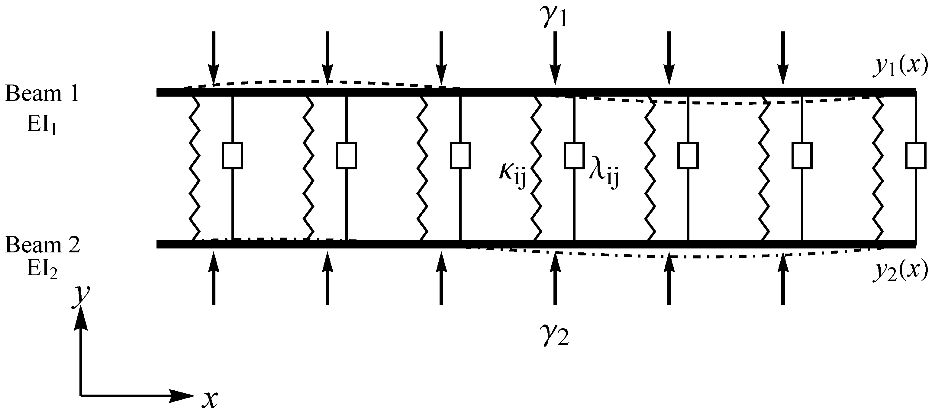
where $E{I}_i$ are bending stiffnesses, ${\kappa }_{ij}$ are elastic couplings, ${\lambda }_{ij}$ are Kelvin–Voigt-type couplings, and ${\gamma }_i$ are aerodynamic damping coefficients; see [22,23] for beam dynamics and damping models. We illustrate this in the following figure.

Figure 1 shows two parallel Euler–Bernoulli beams bending transversely along the longitudinal coordinate x. The beams are connected by distributed springs representing elastic coupling forces proportional to relative displacements, and by dashpots modeling viscoelastic, velocity-dependent damping between them. Additional arrows indicate aerodynamic damping acting on each beam individually. The diagram summarizes how elastic stiffness, internal dissipation, and external drag combine in a coupled fourth-order beam system. The deflections $y_1\left(x\right)$ and $y_2\left(x\right)$ are depicted as dashed and dot-dashed curves, respectively, illustrating the coupled deformation. The depiction of seven distributed elements is a purely schematic choice to provide a good balance and fill the space without being too cluttered; physically, the coupling is continuous (representing infinite springs and dashpots).

We fix the numerical values

$$E{I}_1=2.50,E{I}_2=1.80,$$

$$\left({\kappa }_{ij}\right)=\left[\begin{array}{cc}0& 40.0\\ 40.0& 0\end{array}\right],\left({\lambda }_{ij}\right)=\left[\begin{array}{cc}0& 1.60\\ 1.60& 0\end{array}\right],{\gamma }_1=0.40,{\gamma }_2=0.30,$$

and the external forcing

$$g_1\left(x\right)=0.50sin\left(2x\right),g_2\left(x\right)=0.25cos\left(3x\right).$$

Dividing (10) by $E{I}_i$ yields the explicit system $y^{\left(4\right)}=f(x,y,y^{\prime })$ with

$$f(x,y,y^{\prime })=\left[\begin{array}{c}{f}_1(x,y_1,y_2,y_1^{\prime },y_2^{\prime })\\ f_2(x,y_1,y_2,y_1^{\prime },y_2^{\prime })\end{array}\right],$$

$$f_1(x,y,y^{\prime })=-{\displaystyle \frac{40.0}{2.50}}(y_1-y_2)-{\displaystyle \frac{1.60}{2.50}}(y_1^{\prime }-y_2^{\prime })-{\displaystyle \frac{0.40}{2.50}}{y}_1^{\prime }+{\displaystyle \frac{0.50}{2.50}}sin\left(2x\right),$$

$$f_2(x,y,y^{\prime })=-{\displaystyle \frac{40.0}{1.80}}(y_2-y_1)-{\displaystyle \frac{1.60}{1.80}}(y_2^{\prime }-y_1^{\prime })-{\displaystyle \frac{0.30}{1.80}}{y}_2^{\prime }+{\displaystyle \frac{0.25}{1.80}}cos\left(3x\right).$$

For an initial value formulation (e.g., produced by a shooting approach from a boundary-value setting), we prescribe at $x_0=0$

$$y\left(0\right)=\left[\begin{array}{c}0\\ 0\end{array}\right],y^{\prime }\left(0\right)=\left[\begin{array}{c}0\\ 0\end{array}\right],y^{″}\left(0\right)=\left[\begin{array}{c}1\\ -{\displaystyle \frac{1}{2}}\end{array}\right],y^{‴}\left(0\right)=\left[\begin{array}{c}0\\ 0\end{array}\right].$$

This provides a fully specified vector test problem with explicit velocity dependence, structurally aligned with coupled beam models [22,23].

The zero displacements $y\left(0\right)$ and zero slopes $y^{\prime }\left(0\right)$ indicate that the beams are rigidly clamped at the start. The non-zero second derivatives $y^{″}\left(0\right)$ represent an initial bending moment applied to the supports, where the opposite signs of 1 and $-{\displaystyle \frac{1}{2}}$ imply the beams are bent in opposing directions. This pre-stress generates the subsequent deflection along the beam length. Finally, vanishing $y^{‴}\left(0\right)$ confirms there is no initial shear force at the boundary. The interval of integration was $x\in [0,4]$.

We tested our new pair along with four other conventional Runge–Kutta pairs of orders 6(5). Namely,

1.

T6(5), an FSAL pair presented in [14];

2.

DLMP6(5), an FSAL pair presented in [12];

3.

PD6(5), a pair given in [11];

4.

PTP6(5), an FSAL pair provided in [13].

• T6(5), DLMP6(5) and PTP6(5) are nine-stage pairs that effectively spend only eight function evaluations per step. PD6(5) is an eight-stage pair. Standard Runge–Kutta integration schemes are mathematically formulated exclusively for first-order ordinary differential equations. Consequently, their application to a fourth-order initial value problem, such as $y^{\left(4\right)}=f(x,y,y^{\prime })$, necessitates a structural reformulation. This mathematical procedure transforms the fourth-order equation into a coupled system of four distinct first-order equations. For illustrative purposes, considering a scalar problem paradigm, one introduces auxiliary variables representing the successive derivatives, specifically $y_1=y$, $y_2=y^{\prime }$, $y_3=y^{″}$, and $y_4=y^{‴}$. The original continuous system is equivalently expressed as

  $$y_1^{\prime }=y_2,y_2^{\prime }=y_3,y_3^{\prime }=y_4,y_4^{\prime }=f(x,y_1,y_2).$$

• This reduction protocol inherently quadruples the dimensionality of the state vector undergoing numerical integration. In conclusion, in all cases, we counted the evaluations of f only as an indicator of the computational cost of each pair.

All these pairs were run for tolerances ${10}^{-5},{10}^{-6},\dots ,{10}^{-11}$. All computations were performed using MATLAB [24]. For each tolerance, we recorded the number of stages expended and the endpoint error, since the exact value

$$y\left(4\right)=\left[\begin{array}{c}-9.3412980607233776\\ -3.4183632195980199\end{array}\right]$$

is known. The quantity y(4) denotes the highly accurate reference solution evaluated at the final point of the respective integration interval, specifically $x=4$. This reference value is strictly required to compute the global error at the end of the integration domain achieved by each pair. The computed end-point error is subsequently utilized to quantify the achieved number of accurate digits, which constitutes the performance metric plotted on the vertical axes of the efficiency curves.

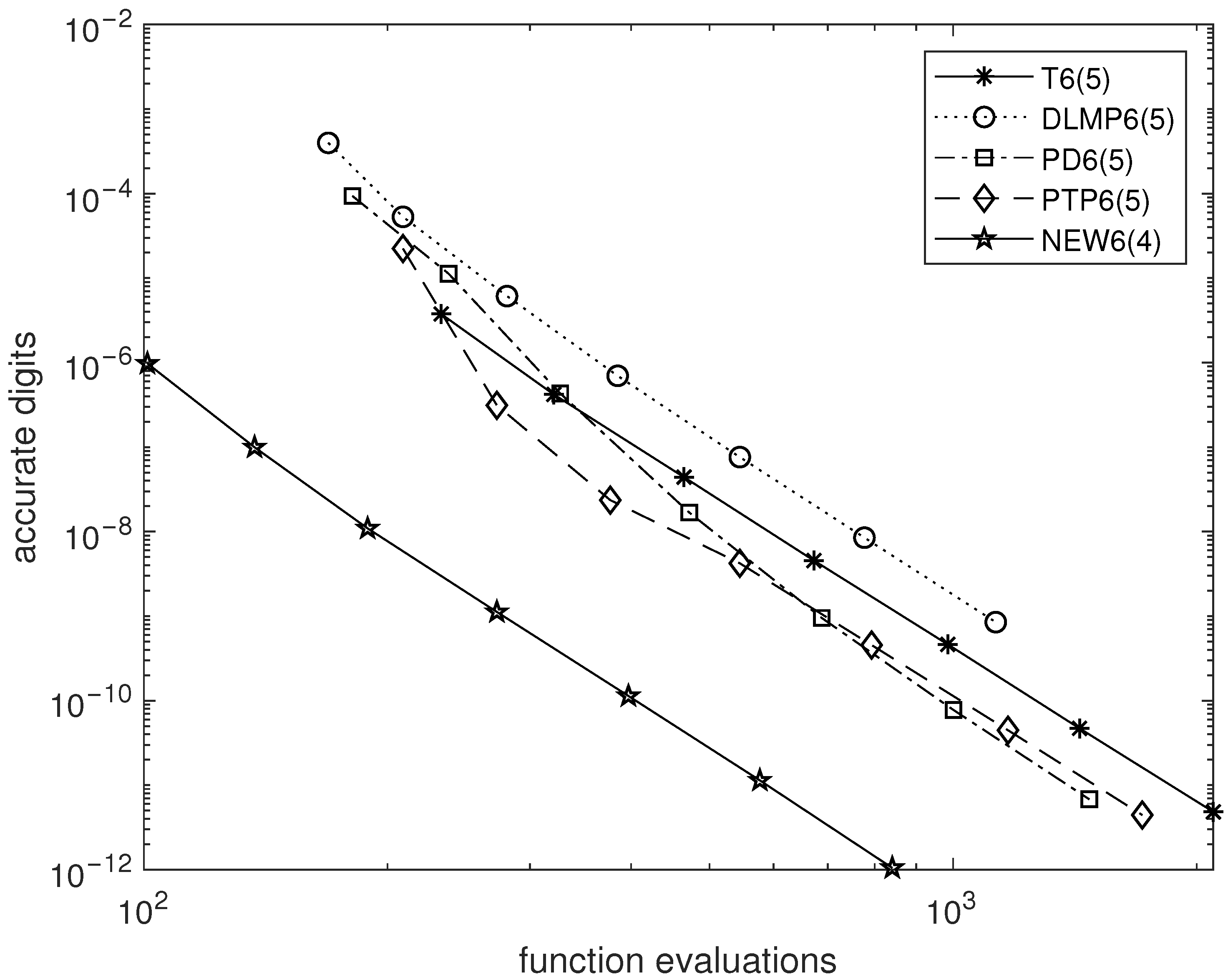
We put all these data in Figure 2 and form the corresponding efficiency curves for each pair. In these representations, the horizontal axis quantifies the computational effort, measured by the cumulative number of function evaluations required to complete the integration interval. The vertical axis denotes the achieved end-point accuracy, expressed as the number of correct digits. The comparability of the numerical schemes is ensured by executing each method across the identical set of strict local error tolerances. The step sizes are dynamically adjusted by the embedded step-size control algorithm to satisfy the prescribed tolerance constraint, guaranteeing a rigorous comparison of the actual computational cost exacted by each pair to achieve a specific level of precision.

We easily verify that our new proposal here gains from $2.5$ to four digits of accuracy, a rather astonishing difference for methods of the same order.

5.2. Problem 2: Modeling Structure–Acoustic Coupling in a Thin-Walled Duct

We consider a one-dimensional vibroacoustic model describing the interaction between a thin elastic duct wall and the acoustic pressure field inside a flow duct.

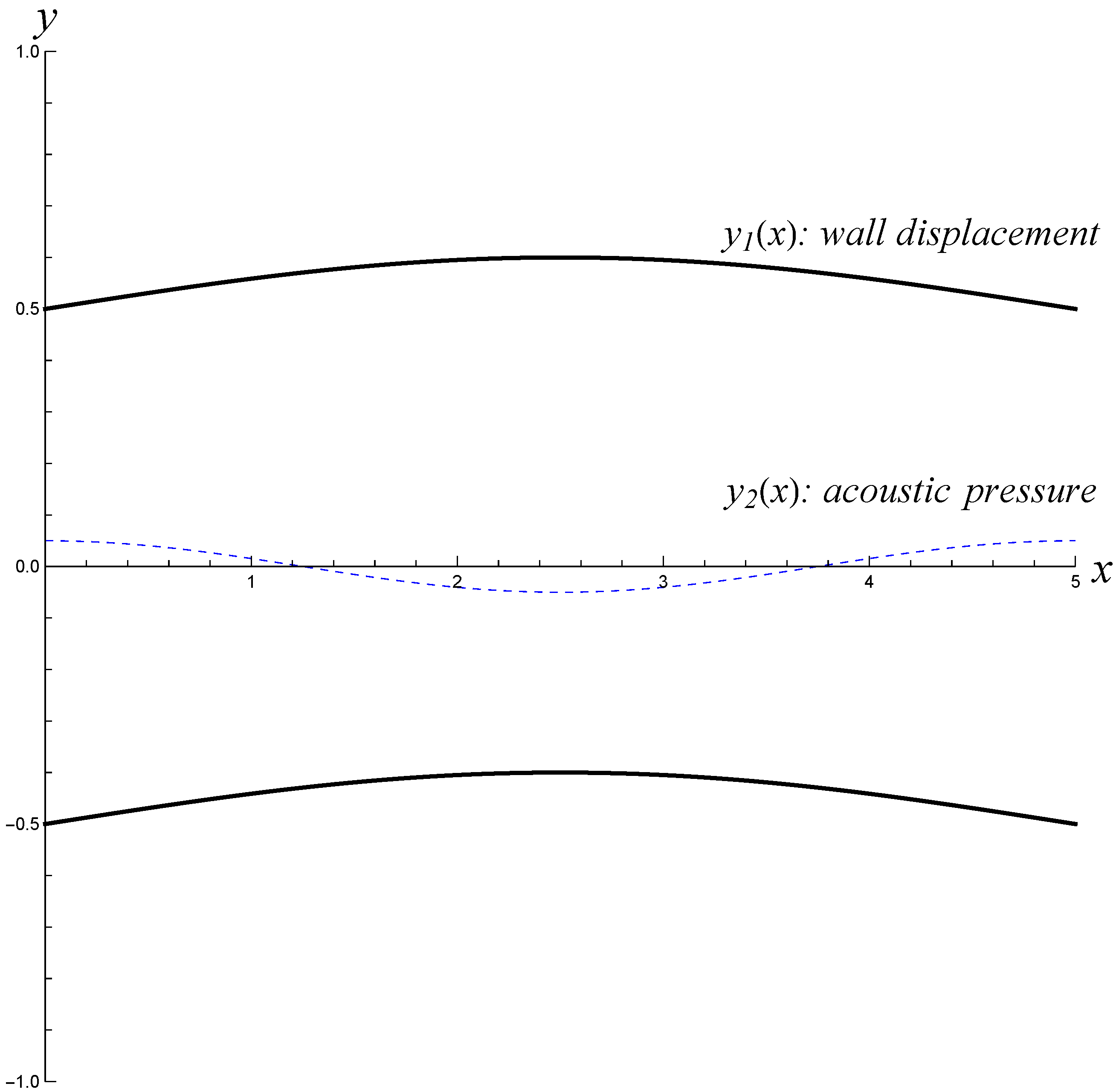
Figure 3 provides a conceptual illustration of this system. The solid lines represent the upper and lower duct walls vibrating transversely according to $y_1\left(x\right)$, while the dashed line shows the acoustic pressure wave $y_2\left(x\right)$ propagating along the duct. The horizontal axis corresponds to the axial position x, and the vertical axis shows the transverse displacement of the walls or the acoustic pressure amplitude y. This figure highlights the qualitative behavior of the coupled system based on the conceptual model used in this work, which captures the essential features of structure–acoustic interaction without requiring a fully detailed physical model. The approach is inspired by classical studies of vibroacoustic interaction in ducts and enclosed cavities [25,26,27,28].

Specifically, the unknown vector

$$y\left(x\right)=\left(\begin{array}{c}{y}_1\left(x\right)\\ y_2\left(x\right)\end{array}\right)\in {\mathbb{R}}^2$$

contains the transverse displacement of the duct wall $y_1\left(x\right)$ and the acoustic pressure amplitude $y_2\left(x\right)$. The coupled governing equations are

$$\left\{\begin{array}{c}{y}_1^{‴\prime }\left(x\right)=-5y_2\left(x\right)-0.8y_1^{\prime }\left(x\right),\hfill \\ y_2^{‴\prime }\left(x\right)=3y_1\left(x\right)-1.2y_2^{\prime }\left(x\right).\hfill \end{array}\right.$$

The system is posed as an initial value problem at the duct inlet $x=0$:

$$\begin{array}{cccccccc}\hfill y_1\left(0\right)& =0.001,\hfill & \hfill y_1^{\prime }\left(0\right)& =0,\hfill & \hfill y_1^{″}\left(0\right)& =0,\hfill & \hfill y_1^{‴}\left(0\right)& =0,\hfill \\ \hfill y_2\left(0\right)& =0.01,\hfill & \hfill y_2^{\prime }\left(0\right)& =0,\hfill & \hfill y_2^{″}\left(0\right)& =0,\hfill & \hfill y_2^{‴}\left(0\right)& =0.\hfill \end{array}$$

The initial values for the coupled vibroacoustic system define the physical state of the duct at the inlet $x=0$ by specifying that the wall begins with a prescribed transverse displacement $y_1\left(0\right)=0.001$ while remaining locally flat and free of internal mechanical stresses, as evidenced by the vanishing slope, bending moment, and shear force represented by the zero values of $y_1^{\prime }\left(0\right)$, $y_1^{″}\left(0\right)$, and $y_1^{‴}\left(0\right)$ respectively. Simultaneously, the acoustic pressure is initialized with an amplitude $y_2\left(0\right)=0.01$, while its spatial derivatives $y_2^{\prime }\left(0\right)$, $y_2^{″}\left(0\right)$, and $y_2^{‴}\left(0\right)$ are set to zero to ensure that the acoustic wave enters the duct with a uniform profile and without abrupt spatial gradients or shocks. Together, these conditions establish a well-defined starting configuration where the structural offset and the initial pressure amplitude can begin to interact through the coupling terms of the governing equations as the solution propagates along the axial length of the duct.

Physically, the first equation models the bending-dominated vibration of the duct wall. The fourth derivative represents wall rigidity, the term proportional to $y_2$ accounts for acoustic loading, and the term proportional to $y_1^{\prime }$ represents aerodynamic damping from the surrounding flow. The second equation describes the axial evolution of the acoustic pressure, with the coupling term proportional to $y_1$ modeling sound generation by the wall motion, and the term proportional to $y_2^{\prime }$ accounting for acoustic energy losses. Together, these equations capture the mutual interaction between structural vibration and acoustic wave propagation in the duct, representing a typical vibroacoustic problem. The interval of integration was $x\in [0,3]$.

Here, we ran our new method along PD6(5) which seemed to perform a little better than other pairs in the previous example. Since the present problem is linear, we also tried ST6(4), a pair that is especially constructed for addressing linear inhomogeneous problems [29]. The latter pair spent only six stages per step. We again ran the selected pairs for tolerances ${10}^{-5},{10}^{-6},\dots$, ${10}^{-11}$ and recorded for each tolerance the stages spent and the end-point error since we know that

$$y\left(3\right)=\left[\begin{array}{c}-0.1524075081008941\\ -4.5138842746137429·{10}^{-3}\end{array}\right].$$

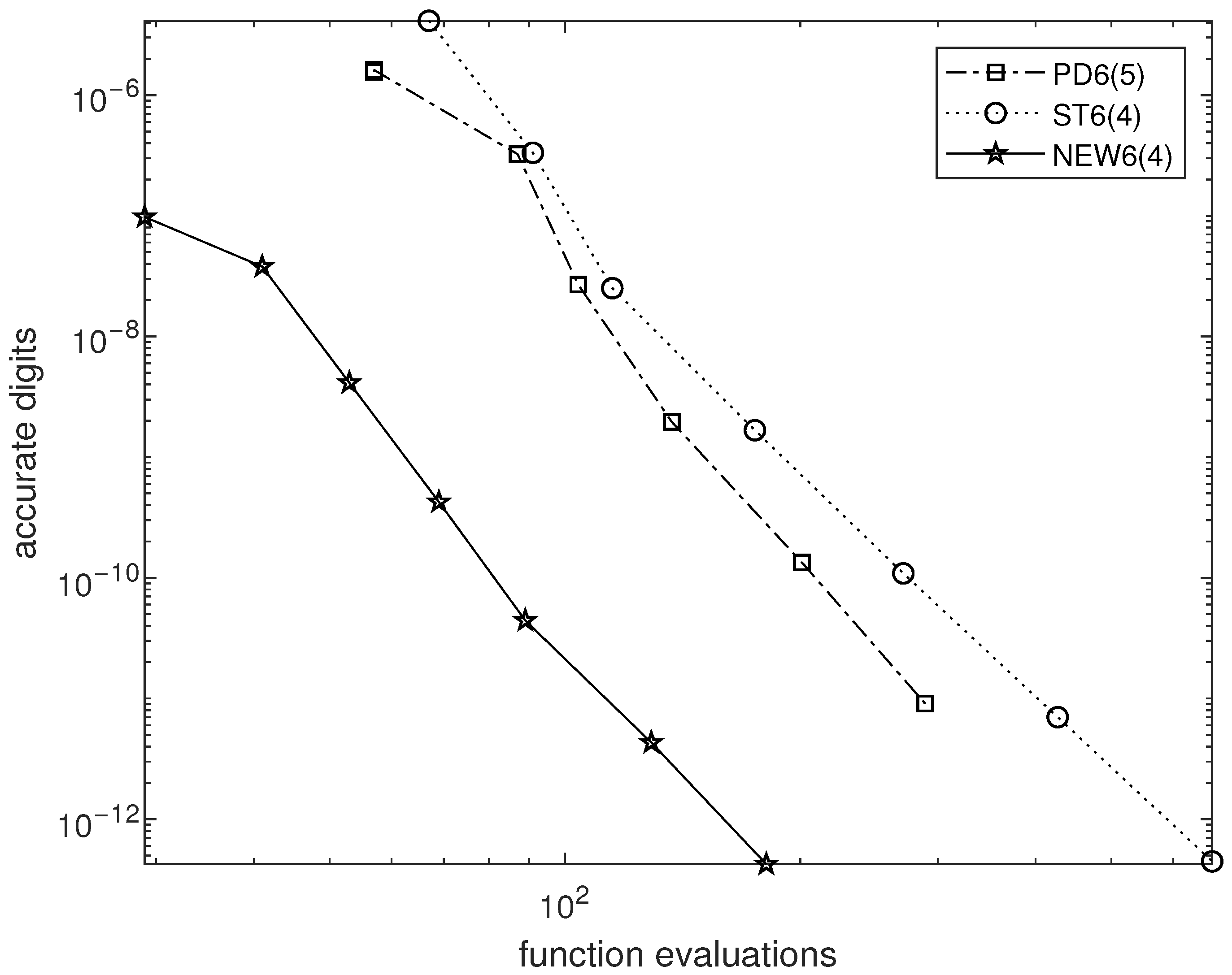
The efficiency curves for these runs are shown in Figure 4. It is clearly verified again that more than three digits of accuracy were gained by our new pair.

6. Conclusions

We established a framework for solving fourth-order ordinary differential equations with explicit dependence on the first derivative, $y^{\left(4\right)}=f(x,y,y^{\prime })$. The derivation of order conditions up to order seven confirmed that the inclusion of the first derivative requires distinct algebraic constraints involving the matrix D, which are absent in classical RKN formulations for $y^{\left(4\right)}=f(x,y)$.

The review of physical applications—spanning structural mechanics, microsystems, and theoretical physics—demonstrates that while many models are idealized to the form $f(x,y)$, realistic descriptions of phenomena such as coupled composite beams and nonlinear foundation interactions often benefit from or require the generality of derivative-dependent formulations. This extension of the RKN method therefore provides a vital tool for the high-precision simulation of a broader class of engineering and scientific problems.