Common Eigenvalues of Vertex-Decorated Regular Graphs

Abstract

Let $G=(V,E)$ be a simple graph with the vertex set V and the edge set E$\left(\left|V\right|=n,\left|E\right|=m\right)$. An example of a vertex-decorated graph $DG$ is a vertex-quadrangulated graph $QG$. The vertex quadrangulation $QG$ of 4-regular graph G visually looks like a graph whose vertices are depicted as empty squares, and the connecting edges are attached to the corners of the squares. If we contract each quadrangle of $QG$ to a point that takes over the incidence of the four edges that were previously joined to this quadrangle, then we can again get the original graph G. Any connected graph H that provides (some of) its vertices for external connections can play the role of a decorating graph, and any graph G with vertices of valency no greater than the number of contact vertices in H can be decorated with it. Herein, we consider the case when G is a regular graph. Since the decoration also depends on the way the edges are attached to the decorating graph, we clearly stipulate it. We show that all similarly decorated regular graphs $DG$ that meet our conditions have at least $\left|V\right(H\left)\right|$ predicted common eigenvalues. A number of related results are proven. As possible applications of these results in chemistry, cases of simplified findings of eigenvalues of a molecular graph even in the absence of the usual symmetry of the molecule may be of interest. This, in particular, can somewhat expand the possibilities of applying the simple Hückel method for large molecules.

1. Introduction

Graph theory has many diverse applications in the natural sciences and other fields. In particular, it has been used quite successfully in chemistry [1,2,3,4,5,6,7,8], where the use of molecular graphs is now firmly established. Studying the properties of molecular graphs helps to study the properties of the molecules themselves and also generates motivation for solving emerging graph-theoretical problems by mathematicians. Herein, we will specifically focus on the spectral approach to graph studies.

In mathematics, spectral graph theory [9,10] is the study of the properties of a graph in relationship to the characteristic polynomials, eigenvalues, and eigenvectors of matrices associated with the graph, such as its adjacency matrix or Laplacian matrix. The foundations of spectral graph theory were laid in the fifties and sixties of the last century. Most of the early results are concerned with the relationship between the spectral and structural properties of a graph, which also serves as an example for modern research, including this work. A detailed and specific bibliography on the topic will be presented by us as we proceed in the main part of the text. However, right now we would like to recommend [9,10,11,12,13,14] as sources of general information. In particular, [11] contains lists of famous lectures, both video recorded and simply written down on paper, by leading experts in the field of graph spectra; collection [12] contains papers on the application of spectral graph theory in a number of practical areas; and [13,14] are specifically devoted to applications in computer science.

For applied purposes, it is appropriate to compare the physical spectra of molecules and the spectra of their graphs. The most characteristic role is played by atomic line spectra, which uniquely represent the corresponding atoms and are widely used in physical methods of analyzing the elemental composition of chemical compounds. Energy (ultraviolet and infrared) spectra of molecules are given in a more complex continuous form, as a curve or broken line. Spectroscopy specialists study the shape of a continuous spectrum in its specific intervals. There are tables compiled on the basis of numerous experiments that present the relationship between atomic groups (radicals) known in (organic) chemistry and the corresponding sections of the physical (UV or IR) spectrum. This allows one to study the chemical structure of compounds. In chemistry, it is a widely used empirical fact that compounds containing identical chemical groups contain similar regions in their physical spectra.

From an informational point of view, the (discrete) spectra of molecular graphs complement physical spectra. When physical spectra are unavailable (e.g., if the corresponding chemical compound has not yet been synthesized), the theoretical graph spectrum can be used to predict the properties of the (imaginary) molecule under consideration. In our topic, an interesting case is when a group of molecules with some common property also has molecular graphs with a common part of their spectra. The practical interest of chemists in such correlations of the properties of molecules with the spectra of their graphs leads to the general mathematical problem of constructing graphs with a common part of the spectra (see [15,16,17,18,19,20,21,22,23,24,25,26] and bibl.).

However, it should be remembered that there is a semantic difference between the spectra of molecular graphs and the physical spectra of the corresponding molecules (taken with the help of spectral instruments). Namely, the former reflect the energy levels of the molecule, while the latter reflect the energies of the transitions between these levels. As long as there are no physical methods that allow researchers to directly determine the energies of the electron levels of a molecule (and not the transitions between them), quantum-mechanical methods of calculating energies, including the approximate methods using molecular graphs, remain the only approaches for assessing these energies.

Herein, we join the work of previous authors [15,16,17,18,19,20,21,22,23,24,25,26] and consider options for constructing families of graphs with a common eigenvalue part. Among the methods used to construct the graphs of interest to us are vertex decoration and the use of suitable graph products. While giving priority to general graph-theoretical reasoning, we also try to point out the possible application of the obtained results in (mathematical) chemistry. In particular, this concerns the calculation of the energy spectrum of molecules using the simple method of the linear combination of atomic orbitals (LCAO) proposed by Hückel. In the course of the presentation, a number of new results of applied significance are proven.

The work included the following stages. The first result defines a necessary spectral condition for a graph to admit rainbow coloring of its vertices. This can be used to search for rainbow graphs in a given large array of graphs. Determining the ranks of graph adjacency matrices by using the standard procedures of matrix theory is much simpler than writing a special program to study the given graphs by computing several of their parameters. For the main topic, k-rainbow-colorable graphs are examples of graphs that have at least $k-1$ common zero eigenvalues $(k\ge 2)$. Further, the main focus is on results related to the construction of not necessarily symmetric graphs obtained by homogeneously decorating the vertices of the original regular graph. The connection of contact vertices occurs according to strictly defined rules; these rules guarantee the existence of a given subspectrum in similarly decorated graphs. The obtained results allow one to consider the decoration of vertices by arbitrary graphs with the required number of contact vertices. This, in particular, includes the decoration of vertices of valency r with r-cycles $(r\ge 3)$, which was previously described only for the cases where $r\le 4$. An example of a graph with cycle-decorated vertices is the skeletal graph of a truncated polyhedron. For the needs of mathematical chemistry, cycle decoration of vertices transforms any, not necessarily regular, graph into a regular graph of chemical valency 3. The substitutional (homogeneous) decoration of graph vertices also simulates the (homo)polymerization process in polymer chemistry. Following the analysis of vertex-decorated graphs, the tensor and Cartesian products of graphs are rigorously described, along with the predicted common portion of their spectra. The study concludes with a consideration of several variants of the restricted rooted product of graphs, including both attaching the decorating graphs via an edge and directly merging the contact vertices of the decorating and decorated graphs.

The transition to the obtained results will require the introduction of strict terminology, which we will move on to in the next part of the text.

2. Preliminaries

We will use the most famous terms of graph theory without reference to sources. Let $G=(V,E)$ be a simple graph with the vertex set V and edge set E$\left(\left|V\right|=n,\left|E\right|=m\right)$. A simpler form of decorating a graph G without removing (replacing) its original vertices is the graph product studied by Godsil and McKay [27]. Let $\mathcal{H}=\{H_1,H_2,\dots ,H_n\}$ be a family of rooted graphs. Then, by $G\left(\mathcal{H}\right)$ we denote the graph obtained by identifying the root of $H_j$ with the j-th vertex of G$(j\in \{1,2,\dots ,n\left\}\right)$. The obtained graph $G\left(\mathcal{H}\right)$ is called the rooted product of G by $\mathcal{H}$ [27] ($G\left(\mathcal{H}\right)$ preserves all original vertices of G and $\mathcal{H}$, too). Interested readers may refer to references [28,29,30,31,32,33,34,35] for more information on this topic. It is also worth mentioning the decoration of graph edges by inserting a certain number of new vertices of valency 2 into them. Two graphs $G_1$ and $G_2$ are called homeomorphic if both can be obtained in this way from some third graph $G_3$ (or one from the other) [36,37]. In particular, the derived graph produced by inserting a degree-2 vertex into each edge of a graph G is called its subdivision (graph) $S\left(G\right)$ [9,10,38,39]; see usage in physical/chemical contexts [40,41].

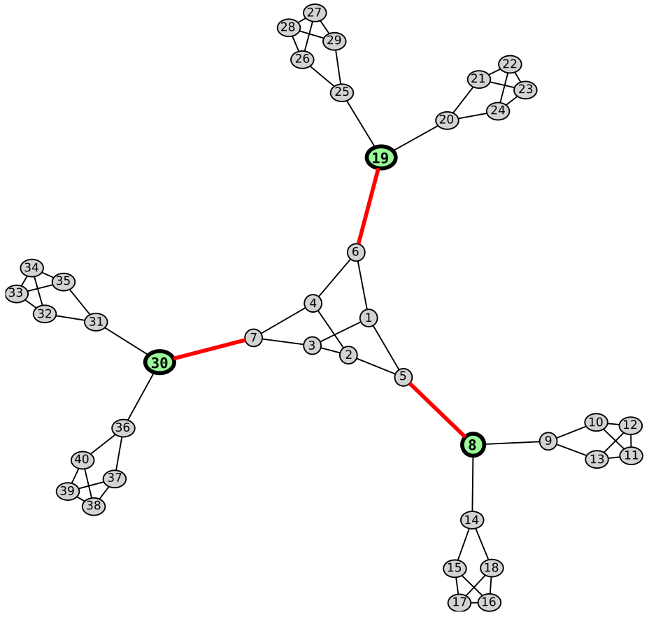
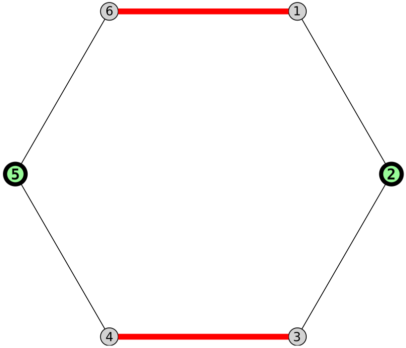
In an arbitrary simple graph H, choose several pairs of different vertices, e.g., $(1, 2), (3, 4)$, suitable for our further reasoning. Then, take n isomorphic copies of H and perform the following operation of joining these copies using edges: connect vertex 1 of each isomorphic copy of H with vertex 2 of any other copy and, similarly, vertex 3 of each copy with vertex 4 of yet another copy. We get an arbitrary (from possible) graph $DG$ consisting of n linked copies of H. If we contract the vertices of each isomorph of H in $DG$ into one vertex (without forming loops), this will give us a 4-regular simple graph G on n vertices. It is important for us that from the compressed graph G we can again obtain the graph $DG$ if we observe the rule of connecting the vertices ($1\&2$ and $3\&4)$ belonging to different copies of the subgraph H in $DG$. This is achieved by corresponding vertex decoration (replacement) of each vertex of the graph G with a copy of the graph H. The result is a ‘polymer’ graph $DG$, assembled from ‘monomer’ copies of graph H using graph G as a plan for connecting them. In what follows, the starting point for us will be the graph G, the vertices of which we will decorate with the graph H to obtain the graph $DG$ (the graph in the problem).

The above principle of connecting ‘monomer’ H-units with contact points designated $1, 2, \dots , r$ generally allows both homogeneous connections (like point 1 of one isomorphic copy of H with point 1 of another copy of H) and heterogeneous contacts (like point 1 of one copy of H with point 2 of another copy, and vice versa). The total number ${\kappa }_r$ of all possible connection schemes (implemented equally for all ‘monomer’ units) is equal to the number of all involutive permutations $\varpi$ of the symmetric group $S_r$ (${\varpi }^2=e$, where e is a unit of $S_r$). The first numbers ${\kappa }_r$ for $r=0, 1, 2, 3, 4, 5, 6, 7$ are $1, 1, 2, 4, 10, 26, 76, 232$, respectively. These numbers can be easily calculated recursively: ${\kappa }_r={\kappa }_{r-1}+(r-1){\kappa }_{r-2}$ [42,43,44]. In the absence of symmetry, ${\kappa }_r$ is also the number of ways to decorate all vertices of the original r-regular graph G in the same way using a decorating graph H with r labeled contact vertices. In the presence of symmetry, ${\kappa }_r$ serves as an upper bound on the number of such nonidentical decorations of all vertices of G using the mentioned graph H with r contact vertices.

There are various kinds of substitutional vertex graph decoration (the elimination of original vertices in exchange for decorating graphs), e.g., stellation, which yields paraline (or para-line) graphs [45,46,47,48,49,50,51,52,53], and vertex quadrangulation [54,55] (consider as a special case a square-octagon lattice [56,57,58,59,60,61,62,63,64,65,66,67,68,69]). In addition, vertex pentangulation, vertex hexangulation [70], vertex heptangulation [71], and more general types of vertex decoration allowing other decorating graphs were studied in [70,72,73,74,75,76,77]. Remember also the example of graphs of truncated polyhedra [78], which illustrates the process of vertex decoration with a cycle whose length equals the valency of the truncated vertex in the graph of the original nontruncated polyhedron. The term vertex truncation is also used as a synonym when referring to decorating the vertices of an arbitrary graph (not necessarily a polyhedral one) with cycles [70,71,72,73,74,75,76,77,79]. Moreover, the term generalized vertex truncation is used by some authors to refer to any sort of vertex decoration (not necessarily with cycles) [70,72,73,74,75,76,77].

We now turn from constructional questions to spectral ones. The characteristic polynomial $\mathrm{Ch}(G;x)$ of an arbitrary graph G is defined as the characteristic polynomial $\mathrm{Ch}(G;A)$ of its adjacency matrix $A=A\left(G\right)$ [9,10]:

$$\mathrm{Ch}(G;x):=\mathrm{Ch}(A;x)=det(xI-A),$$

(1)

where I is the identity matrix of the corresponding dimension. The spectrum $\mathrm{Sp}\left(G\right)=\{{\lambda }_1, {\lambda }_2, \dots , {\lambda }_n\}$ $({\lambda }_1\ge {\lambda }_2\ge \cdots \ge {\lambda }_n)$ of a graph G is the multiset of all eigenvalues ${\lambda }_j$$\left(j\in \{1, 2, \dots , n\right)$ of its adjacency matrix A, or all the roots of the characteristic polynomial $\mathrm{Ch}(G;x)\equiv \mathrm{Ch}(A;x)$ [9].

For an arbitrary square matrix $A={\left[a_{ij}\right]}_{i,j=1}^n$, there are $2^n$ ways to simultaneously partition all columns and rows of A into rectangular blocks. In the last, the original matrix A is used in two different ways: as a block matrix with $n^2$ $1\times 1$ blocks and A itself, which is one $n\times n$ block. For our purposes, out of all the $2^{2n}$ rectangular partitions of A, a simultaneous row and column partition will primarily be used, because only such a partition makes all diagonal blocks square blocks.

Let $B={\left[B_{kl}\right]}_{k,l=1}^q$$\left(q\in \{1, 2, \dots , n\}\right)$ be an arbitrary block partition of the matrix A, where the role of the entry $B_{kl}$ is played by the whole block $B_{kl}$ of A. For an arbitrary $p_k\times p_l$$\left(p_k,p_l\le n\right)$ block $B_{kl}$ of B, calculate the sums ${\rho }_t={\sum }_{u=1}^{p_l}{b}_{tu}$ of entries in rows, where the sum ranges over all $p_l$ entries $b_{tu}$ of the t-th row of $B_{kl}$. (Recall that the entries $b_{tu}$ of $B_{kl}$ are the corresponding entries $a_{ij}$ of A. But we do not consider this here.)

In general, the row entry sums ${\rho }_1, {\rho }_2, \dots , {\rho }_{p_k}$ may be different (numbers), for an arbitrarily chosen or even each block $B_{kl}$ of A (res. block-entry of B). Herein, a crucial role is played by block partitioning into such blocks, if any, where all row sums ${\rho }_t$ are equal to ${\rho }_{B_{kl}}=\mathrm{const}\left(B_{kl}\right)$ in each block, although different blocks may have different row entry sums ${\rho }_{B_{kl}}$’s.

We emphasize that, in the general case, an arbitrary matrix A (especially an adjacency matrix) does not guarantee a partition into $p_k\times p_l$$\left(p_k\ge 1,p_l\ge 2\right)$ blocks $B_{kl}$ so that each of them has a common value ${\rho }_{B_{kl}}$ of its row entry sums. However, quite often, a simple change in the numbering of rows (columns) or, in other words, the simultaneous rearrangement of rows and columns results in such a partition. Moreover, in this way we can sometimes get different partitions that satisfy our discussed conditions.

A well-known example of matrix partitioning is one that uses symmetry considerations to group row (column) indices. In this case, each set of indices numbering rows (columns) of the whole block $B_{kl}$ is an orbit of indices induced by the automorphism (symmetry) group $\mathrm{Aut}\left(A\right)$ of A. A subgroup $U\subseteq \mathrm{Aut}\left(A\right)$, in the general case, can induce a partition into its own orbits, generating the same or other orbits obtained by splitting those orbits induced by $\mathrm{Aut}\left(A\right)$.

We come to the general situation in which some symmetry may or may not play a role. Recall that any partition of A into blocks with common row sums ${\rho }_{B_{jk}}$ is an example of an equitable partition of matrix entries [80,81,82,83,84,85,86,87,88]. Accordingly, an equitable partition of a simple graph G is a partition of its vertex set V into parts $V_1, V_2, \dots , V_s$, such that (a) the vertices of each part $V_i$ induce a regular graph (possibly empty) and (b) the edges between $V_i$ and $V_j$ induce a semiregular graph (possibly regular or empty). In general, there may be different equitable partitions of the same graph that satisfy this definition. Note here that symmetry can only work with orbits of equal entries. However, the condition imposed on equal row entry sums in a block does not mean that rows with equal entry sums must necessarily contain equal entries. A common value of the sum ${\rho }_{B_{kl}}$ may be associated with different entries in row. Let us say that 10 is the sum $5+0+5$, but it is also the sum of $1+19+(-10)$, and there are infinitely many other additive representations of 10.

Herein, we are interested in just the equitable partition, since in the general case it can exist even in the absence of any symmetry (of our matrix or graph).

Let B be an equitable block partition of A. And let $\mathcal{B}={\left[b_{B_{kl}}\right]}_{k,l=1}^q$ be the matrix whose entries $b_{B_{kl}}$ are the common row entry sums of blocks $B_{kl}$$\left(k,l\le q;q\in \{1, 2, \dots , n\}\right)$. We may now show that equitable block partitions of a matrix A are really special. Using our notation, we present here the famous theorem from matrix theory (see [89,90] or Theorem 012 in [9]):

Theorem 1 

([89,90]). Let $B={\left[B_{kl}\right]}_{k,l=1}^q$ be an equitable block partition of a matrix A. Also, let $\mathcal{B}={\left[b_{B_{kl}}\right]}_{k,l=1}^q$ be the matrix whose entries $b_{B_{kl}}$ are the common row entry sums of blocks $B_{kl}$ of A (entries of B). Then, the spectrum of the eigenvalues of $\mathcal{B}$ is contained in the spectrum A (taking into account all multiplicities of eigenvalues).

Remark 1.

It is essential to note that the type of the matrix A in Theorem 1 does not imply that $\mathcal{B}$ is also of the same type. E.g., a Hermitian (res. symmetric) matrix A may have a non-Hermitian (res. nonsymmetric) divisor $\mathcal{B}$ (and vice versa). The matrix $\mathcal{B}$ can be viewed as a weighted matrix of a weighted digraph Γ (possibly with loops) or, if it is a symmetric nonnegative integer matrix, it can also represent a multigraph with parallel unweighted edges.

In other words, Theorem 1 states that the characteristic polynomial $\mathrm{Ch}(\mathcal{B};x)$ of a matrix $\mathcal{B}$ divides the characteristic polynomial $\mathrm{Ch}(A;x)$ of a matrix A. This is why the matrix $\mathcal{B}$ is called a (front) divisor (or quotient matrix) of the matrix A [86,89,90,91]. Similarly, the weighted (di)graph $\Gamma \left(\mathcal{B}\right)$ with $\mathcal{B}$ as its weighted adjacency matrix is called a (front) divisor (or quotient graph) of the graph G [9,10,91], with A as the adjacency matrix (see applications [54,55]). We can also universally call either of the two divisors simply divisor. Usually, there can be no contradiction, since the (weighted) graph and its (weighted) adjacency matrix uniquely represent each other. An example of a divisor graph $\Gamma \left(\mathcal{B}\right)$ is the graph of the unit cell of a crystal with periodic (cyclic, toroidal) boundary conditions (see [92,93]). Such cells have long been used in solid state physics to calculate the energy bands in crystalline solids [93]. In addition, note that the quotient graph $\Gamma \left(\mathcal{B}\right)$ is a weighted homomorphic image of the original graph G (see graph homomorphisms as the principal topic in [94]).

Let ${\lambda }_j$ and ${\mathfrak{v}}_j=(s_{1j}, s_{2j}, \dots , s_{nj})$ be an eigenvalue and the corresponding eigenvector of an arbitrary $n\times n$ matrix M; $j\in \{1, 2, \dots , n\}$. If the vector ${\mathfrak{v}}_j$ is not orthogonal to the n-vector $(1, 1, \dots , 1)$ of all ones, or, equivalently, ${\sum }_{i=1}^n{s}_{ij}\ne 0$, then ${\lambda }_j$ is called a main eigenvalue of M [95,96] (see pp. $46,107,142$ in [9]). In general, M can have more than one main eigenvalue. Of particular interest to us is that the number of main eigenvalues of the adjacency matrix A of a graph G is at most the number of orbits generated by its automorphism group $\mathrm{Aut}\left(G\right)$ on the vertex set $V\left(G\right)$ or of any other orbits (e.g., generated by an equitable partition); see Theorem 4 in [96] together with Theorem 1 in [95] or with Theorem 1 in [96]. Thus, the number of main eigenvalues is a lower bound on the minimum possible number of vertex orbits of G and an estimate of the degree of symmetry of G when the orbits are generated by its automorphism group $\mathrm{Aut}\left(G\right)$ or by its semigroup (monoid) $\mathrm{End}\left(G\right)$ of strict endomorphisms (see [97,98]). Let us say that a vertex-transitive graph G (all of whose vertices are symmetrically equivalent and form only one orbit) can have only one main eigenvalue (equal to a common valency of its vertices), while a graph with ‘many’ main eigenvalues will have a larger number of equivalence classes of vertices (where vertices from different classes are not symmetrically equivalent). As an example, the vertex-quadrangulated graphs $QG$ with equitable partitions of their vertices into four orbits, previously studied in [54,55], can have at most four main eigenvalues. In fact, as a 3-regular graph, $QG$ has only one main eigenvalue, 3.

The topic we are considering echoes with the topic of coloring the vertices and/or edges of graphs. A proper vertex (edge) k-coloring of G is defined as a vertex (edge) coloring from a set of k colors such that no two adjacent vertices (edges) share a common color. The chromatic number $\chi \left(G\right)$ (chromatic index ${\chi }^{\prime }\left(G\right)$) is the smallest number of colors needed for a proper coloring of the vertices (edges) of a graph G. Another type of coloring has only attracted attention in recent decades; it is, as it were, one step back from proper coloring. This is a rainbow coloring (of vertices) in which each vertex of the r-regular graph has exactly one adjacent vertex of each of the fixed (for all vertices) r colors, including its own color (see [99] and bibl.). For example, when a red vertex in a (cubic) 3-regular graph has exactly one adjacent vertex in green, one in yellow, and one in its own red; and this same coloring method is repeated up to color permutation for all vertices.

However, not all regular graphs can be rainbow colored, only those that satisfy a certain set of properties, summarized in the following statement, given here in its original form of Proposition 1.1 in [99]:

Proposition 2 

([99]). Let Γ be a rainbow graph with v vertices and e edges, and let $\pi :V\left(\Gamma \right)\mapsto C$ be a rainbow coloring of Γ. Then, the following hold.

(a) 

Γ is k-regular, where k is the size of the color set C.

(b) 

Γ contains a perfect matching.

(c) 

Each color $c\in C$ occurs equally often in $(\Gamma ;\pi )$.

(d) 

$k\mid v$ and $k^2\mid e$.

(e) 

For any subset $C^{\prime }$ of C the induced subgraph $\Gamma \left[V^{\prime }\right]$, where $V^{\prime }={\pi }^{-1}\left(C^{\prime }\right)$, is a rainbow graph with rainbow coloring ${\pi |}_{V^{\prime }}:V^{\prime }\mapsto C^{\prime }$.

Remark 2.

Note that the second assertion, $k^2\mid e$, of (d) in Proposition 2 is stronger than the first, $k\mid v$, and implies it. Since (in terms of Proposition 2) $e=kv/2$, the second statement can be rewritten as $k^2\mid kv/2$, which is reduced to $2k\mid v$ and thus is stronger than $k\mid v$. Moreover, if the first four conditions (statements) (a)–(d) of Proposition 2 are satisfied, the last fifth assertion (e) also similarly holds for all $k^{\prime }$-colored $k^{\prime }$-regular $C^{\prime }$-induced subgraphs of Γ, where $k^{\prime }=\left|C^{\prime }\right|\ge 3$$(C^{\prime }\subseteq C)$, while the case $|C^{\prime }|=2$ is possible only if $C^{\prime }$-induced subgraph $\Gamma \left[V^{\prime }\right]$ is a disjoint union of cycles of evenly even lengths (divisible by 4).

In connection with the subsequent application of Proposition 2, recall the following definitions. An s-matching of a graph G is the set of its s nonincident edges $(0\le s\le \lfloor n/2\rfloor )$. A perfect matching $\mathcal{M}$ of a graph G on an even number n of vertices is the set of $n/2$ nonincident edges of G that cover all of its vertices.

Here, we will move on to the main part of our text, where we will continue the previous study of the spectra of vertex-decorated graphs [54,55].

3. The Main Part

We begin by extending the list of properties of rainbow graphs given in Proposition 2 of Woldar [99] by adding one more.

Proposition 3.

Let Γ be a rainbow graph with v vertices and e edges, and let $\pi :V\left(\Gamma \right)\mapsto C$ be a rainbow k-coloring of Γ. Let also Γ satisfy items (a)–(e) of Proposition 2. Then, the spectrum of Γ contains an eigenvalue $\lambda =k$ (as any k-regular graph) and at least $k-1$ eigenvalues $\lambda =0$.

Proof. 

Since each vertex of $\Gamma$ has exactly one adjacent vertex of each of the k colors (including its own color), the adjacency matrix $A\left(\Gamma \right)$ of $\Gamma$ has a divisor J, which is a principal $k\times k$ submatrix of all 1’s, having the spectrum $\mathrm{Sp}\left(\Gamma \right)=\{k, 0^{k-1}\}$. Whence the proof follows. □

Thus, if and arbitrary unweighted graph $\Gamma$ has less than $k-1$ zero eigenvalues, it cannot be a k-colorable rainbow graph. In particular, if Γ has no zero eigenvalues, it cannot be a rainbow graph for any k.

Proposition 3 allows one to determine the common part of the spectra of all k-colored rainbow graphs, which is a challenging task in itself, but it does not allow one to determine the full spectrum of such a graph. However, some rainbow graphs from among paraline graphs (clique-inserted graphs) [45,46,47,48,49,50,51,52,53] $CG$ (a special case of $DG$) are graphs whose spectrum is completely determined by an independent method if the characteristic polynomial (or spectrum) of G is known. An example is the paraline graph $CG$ of an r-regular graph G with r edge-disjoint perfect matchings ${\mathcal{M}}_1, {\mathcal{M}}_2, \dots , {\mathcal{M}}_r$ $({\cup }_{j=1}^r{\mathcal{M}}_j=G; {\chi }^{\prime }\left(G\right)=r)$, which $\left(G\right)$, particularly for an even number r, can be a bipartite Eulerian graph. In the paraline graph $CG$ that we construct, all edges of every perfect matching ${\mathcal{M}}_j$ of G become edges connecting copies of the complete graph $K_r$. We will show that the graph $CG$ obtained in this way is indeed a rainbow graph by proving the following statement:

Proposition 4.

Let $CG$ be the paraline graph of an r-regular graph G with r edge-disjoint perfect matchings ${\mathcal{M}}_1, {\mathcal{M}}_2, \dots , {\mathcal{M}}_r$ $({\cup }_{j=1}^r{\mathcal{M}}_j=G; {\chi }^{\prime }\left(G\right)=r)$. Then, $CG$ has a rainbow r-coloring (i.e., is a rainbow graph).

Proof. 

Color all edges of each connecting n-matching ${\mathcal{M}}_j$ $(j\in \{1, 2, \dots , r\left\}\right)$ in one chosen color, which different from the color of the edges in other such matchings. Further, color all vertices of $CG$ in the colors of edges incident to them. As a result, all pairwise adjacent vertices belonging to any copy of the complete graph $K_r$ are colored in different colors, and the adjacency of vertices through which any two adjacent copies of $K_r$ are connected are colored in one common color. This satisfies the definition of a rainbow r-coloring. The proof is complete. □

Corollary 4.1.

Let $CG$ be the paraline graph of an r-regular bipartite Eulerian graph G. Then, $CG$ is an r-colorable rainbow graph that has at least $r-1$ zero eigenvalues.

Proof. 

By the famous 2-factor theorem (see [100]) discovered by Petersen, every r-regular bipartite Eulerian graph G $(r=2s)$ can be partitioned into s edge-disjoint 2-factors (being in our case spanning subgraphs each component of which is a cycle of even length). Since a cycle of even length has two edge-disjoint perfect matchings, every 2-factor has at least two perfect matchings. Thus, all the s 2-factors contain at least one set $\{{\mathcal{M}}_1, {\mathcal{M}}_2, \dots , {\mathcal{M}}_r\}$ of r edge-disjoint perfect matchings of G. By Proposition 4, $\Gamma$ is an r-colorable rainbow graph, and, by Proposition 3, it has at least $r-1$ zero eigenvalues. This completes the proof. □

The characteristic polynomial $\mathrm{Ch}(CG;x)$ of the paraline graph $CG$ of an r-regular graph [45,46,47,48,49,50,51,52,53] is calculated by Formula (9) given in [45] for $P_{L_2\left(G\right)}\left(\lambda \right)$, which denotes our $\mathrm{Ch}(CG;x)$ below:

$$\mathrm{Ch}(CG;x)={\left[x(x+2)\right]}^{m-n}\mathrm{Ch}(G;x^2-(r-2)x-r),$$

(2)

from where the spectrum of $CG$ can be computed by solving the equation $\mathrm{Ch}(CG;x)=0$ (R.H.S. of $\left(2\right)$ equated to 0). From (2), it is seen that $CG$ has at least $m-n$ zero eigenvalues, which for all $r\ge 3$ is greater than the lower bound $r-1$ estimated by Proposition 3. For $r=2$, $m-n=0$ and $CG$ is an evenly even cycle of length $4s$, which has 2 zero eigenvalues $(2>r-1=1>m-n=0)$. For $r=1$, $m-n=1-2=-1$ and $CG=C{K}_2=K_2$, which has no zero eigenvalue $(r-1=0>m-n=-1)$.

Paraline graphs of molecules, in particular, have applications in modern theoretical chemistry, where spectral aspects of graph theory play an important role [47,48,49,50,51]. These are decorated graphs that are relatively easy to study. However, now, we want to focus on a more general form of vertex-decorated graph $DG$ in which an arbitrary connected graph H is used to decorate the vertices of the original graph G. Such $DG$ graphs are not rainbow graphs in general, but we will use some of the general considerations we presented above for the latter case.

Let H again be a decorating graph with r$(r\le |V\left(H\right)\left|\right)$ contact vertices marked with numbers $1, 2, \dots , r$. Recall that marking the vertices is necessary both to designate vertices of different types and to take into account their relative position in the graph (even if they are equivalent; for example, to give a fixed cyclic order of their sequence in the cycle). In our text, we will consider only uniform decoration of the vertices of the original graph G, when the condition of connecting the vertex of each decorating copy of H with the vertex of another copy of H is specified by a fixed involutive permutation $\varpi =\left(\begin{array}{cccc}1& 2& \cdots & r\\ j_1& j_2& \cdots & j_r\end{array}\right)$ $(\{j_1, j_2, \dots , j_r\}=\{1, 2, \dots , r\})$, where the reversible correspondence $s\iff j_s$ means that the contact vertex s of one copy of H is connected to the vertex $j_s$ of another copy of H (according to the construction of decorated graph G), and vice versa.

Naturally, the simplest case is decoration that corresponds to the identity permutation $\varpi =\left(\begin{array}{cccc}1& 2& \cdots & r\\ 1& 2& \cdots & r\end{array}\right)$, which specifies that a vertex of each copy of H labeled s is connected only to a vertex of the same type s of another copy; $s\in \{1, 2, \dots , r\}$. One example is the case (discussed above) where the resulting graph $DG$ is a rainbow graph. In the case where $H=K_3$ (triangle), coloring the vertices of each of the triangles in three different colors allows us to connect vertices of the same colors belonging to different triangles. (The graph $K_{3}G$ obtained by such decoration is also a paraline graph.) However, in general (rainbow and nonrainbow cases), the coloring of the contact vertices of the graph in different colors is suitable for our topic, provided that only vertices of the same or two distinct, but ‘linked’ in a pair, colors are connected.

The study of the spectra of r-regular graphs after decorating their vertices with cycles of the appropriate length has hardly gone beyond quadrangulations of 4-regular graphs [54,55]. Cases of decoration with cycles of lengths of 5 or more have been practically unstudied. Even in the mentioned case of quadrangulation, not everything has yet been investigated. In particular, it is known that on a set (of graph vertices), in the general case, there can be more than one equitable partition and, as a consequence, there can be different divisors of the graph (characteristic polynomial) with different spectra. This adds to the already discovered obligatory eigenvalues additional ones that the graph $QG$ must have.

Previously [54,55], the eigenvalues $\{3, {(-1)}^3\}$ (spectrum of the complete graph $K_4$ or the skeletal graph of the tetrahedron) and $\{3, 1^3, {(-1)}^3, -3\}$ (spectrum of the cube graph) in bipartite graphs $QG$ were studied, where the superscripts indicate the multiplicity of corresponding eigenvalues. Here, we make a small addition to [54,55] for the case when the original 4-regular graph G has ${\chi }^{\prime }=4$ and all 4-cycles in the vertex-quadrangulated graph $QG$ can be colored with four different colors in the same cyclic order for them or in two opposite orders for different cycles, so that each edge connecting two 4-cycles is incident to vertices of the same color. Then, in the case of the decorating graph $H=C_4$ with adjacency matrix $A\left(C_4\right)$ and its spectrum $\mathrm{Sp}\left(A\right)=\{2, 0^2, -2\}$ there exists another divisor with adjacency matrix $\mathcal{B}$:

$$A\left(C_4\right)=\left[\begin{array}{cccc}0& 1& 0& 1\\ 1& 0& 1& 0\\ 0& 1& 0& 1\\ 1& 0& 1& 0\end{array}\right]\Rightarrow \mathcal{B}=\left[\begin{array}{cccc}1& 1& 0& 1\\ 1& 1& 1& 0\\ 0& 1& 1& 1\\ 1& 0& 1& 1\end{array}\right],$$

(3)

with spectrum $\mathrm{Sp}\left(\mathcal{B}\right)=\{3, 1^2, -1\}$, which adds two more obligatory eigenvalues equal to 1 to those that were found for nonbipartite graphs $QG$ [54,55]. The matrix $\mathcal{B}$ is the adjacency matrix of the divisor graph $\Gamma \left(\mathcal{B}\right)$; its diagonal unit entries indicate the adjacency of vertices with the same label (of the same color) described above (in particular, when considering the rainbow coloring of rainbow graphs). If the vertices of an r-regular r-edge-colorable graph G are decorated with cycles of length r (using all r vertices for contacts, each for contact with a vertex of the same color), then the resulting decorated graph $C_{r}G$ is an edge-disjoint union of perfect m-matching and n disjoint copies of the r-cycle, where $m=rn/2$ and n are the number of edges and vertices of G, respectively.

Here, we make some generalization to the case of quadrangulation considered in this text (not taken into account in previous works).

Lemma 5.

Let the decorated graph $C_{r}G$ (defined above) be cellularly embedded in a surface so that all decorating r-cycles in it are faces on this surface and can be colored with the same set of r different colors, arranged in the same cyclic order or in two opposite orders for different cycles so that each edge connecting two face r-cycles is incident to vertices of the same color. Then, $C_{r}G$ has a divisor graph $\Gamma \left(\mathcal{B}\right)$ with an $r\times r$ adjacency matrix $\mathcal{B}$ that has an all-ones diagonal:

$$\mathcal{B}=\left[\begin{array}{ccccc}1& 1& 0& \cdots & 1\\ 1& 1& 1& \cdots & 0\\ 0& 1& 1& \cdots & 0\\ ⋮& ⋮& ⋮& \ddots & 0\\ 1& \cdots & \cdots & 1& 1\end{array}\right]=A\left(C_r\right)+I_r,$$

(4)

where $A\left(C_r\right)$ and $I_r$ are the adjacency matrix of an r-cycle and the identity matrix of the dimension $r\times r$, respectively.

Proof. 

First, label the vertices in each cycle with numbers $1, 2, \dots , r$, so that adjacent vertices of r-cycles connected by an edge have the same labeling number. Next, we renumber all the vertices of the graph $C_{r}G$ so that, first, all n vertices that previously had the number 1 are numbered, then all vertices marked 2, …, and so on through r inclusive. The adjacency matrix with such numbering of vertices is divided into r-by-r blocks of two types, consisting of only zeros and containing exactly one unit in each row and each column (because each vertex of a cycle has exactly one adjacent vertex in some other cycle). Replacing zero blocks with zeros and blocks containing units with ones leads to the derivative $r\times r$ $(0, 1)$-matrix, which is exactly the matrix $\mathcal{B}$. □

Corollary 5.1.

Let $C_{r}G$ be as in Lemma 5. Then, $C_{r}G$ has r obligatory eigenvalues $\{\lambda \mid \lambda =1+\cos ({\displaystyle \frac{2\pi j}{r}}); j=0, 1, \dots , r-1\}$ belonging to the matrix $\mathcal{B}$.

Also, we present here the following obvious corollary.

Corollary 5.2.

The divisor graph $\Gamma \left(\mathcal{B}\right)$ corresponding to the adjacency matrix $\mathcal{B}$ in Lemma 5 has a loop of weight 1 attached to each vertex.

Note that Lemma 5 and Corollaries 5.1 and 5.2, as formulated above (for a fixed cellular embedding of $C_{r}G$ in a surface), are universal and do not depend on the nature of the r-regular graph G but only on the valency r of its vertices and the labeling of the r-cycle $C_r$ (which is circular in this case).

Now, we turn to the consideration of the most general case in this particular work, when the vertices of an r-regular graph G are decorated by an arbitrary connected graph H$\left(\right|V\left(H\right|)\ge r)$ with a fixed choice of r vertices for contact connections. What the divisor graph $\Gamma \left(\mathcal{B}\right)$ of the resulting union of isomorphic copies of the graph H will look like will depend on the choice of a particular uniform decoration scheme. In general, it may contain both new edges and loops added to a copy of the graph H as a result of connections between the contact vertices of different copies of H. We will consider loops as degenerated edges whose end vertices coincide (while the general notation $jk$ of an edge reduces to $jj$ by its form). As we have already indicated above, for a given numbering of contact vertices in a graph H, the procedure for decorating the vertices of the graph G is completely determined by the involutive permutation $\varpi =\left(\begin{array}{cccc}1& 2& \cdots & r\\ j_1& j_2& \cdots & j_r\end{array}\right)$ $(\{j_1, j_2, \dots , j_r\}=\{1, 2, \dots , r\})$ acting on the set of numbers of contact vertices. Any permutation $\varpi$ of r symbols has an equivalent representation as an $r\times r$ permutation (0,1)-matrix $M_{\varpi }={\left[{\mathfrak{a}}_{st}\right]}_{s,t=1}^r$, which has exactly one 1 in each row and each column. The matrix entry is determined by the rule

$${\mathfrak{a}}_{st}=\left\{\begin{array}{c}1\mathrm{if}t=j_s,\hfill \\ 0,\mathrm{otherwise}\hfill \end{array}\right.(s, t=1, 2, \dots , r).$$

(5)

Let the contact vertices in the graph H correspond to the first r numbers $(r\le |V\left(H\right)\left|\right)$ among the numbers of its vertices. We construct an auxiliary augmented matrix $U_H={\left[{\mathfrak{u}}_{st}\right]}_{s,t=1}^{\left|V\right(H\left)\right|}$, in which the upper diagonal $r\times r$ block is the permutation matrix $M_{\varpi }$, and all other entries are equal to 0. The matrix $U_H$ is symmetric: ${\mathfrak{u}}_{st}={\mathfrak{u}}_{ts}$ (since $\varpi$ is involutive permutation, which implies that $M_{\varpi }$ is symmetric). Obviously, the identity entries of $U_H$ correspond to the adjacencies of contact vertices of one copy of the graph H with contact vertices of its neighbors. Specifically, the entry ${\mathfrak{u}}_{st}=1$ indicates the adjacency of vertex s with vertex t in two corresponding adjacent copies of H. In the case $s\ne t$, this creates an edge $st$ in the divisor graph $\Gamma \left(\mathcal{B}\right)$; in the case $s=t$, it creates a loop $tt$ in it. From what has been written, we can formulate the following technical result regarding our example, which generalizes (4) belonging to Lemma 5:

Lemma 6.

The matrix divisor $\mathcal{B}$ of the divisor graph $\Gamma \left(\mathcal{B}\right)$ is $\mathcal{B}=A\left(H\right)+U_H$.

Since we know how to construct the matrix $\mathcal{B}$, we recall why we need it by generalizing Lemma 5 with the following:

Proposition 7.

Let $DG$ be the graph obtained by homogeneously decorating the vertices of an arbitrary r-regular r-edge-colorable graph G with an arbitrary labeled graph H with r vertices for contacts, according to the permutation ϖ. Also, let $\Gamma \left(\mathcal{B}\right)$ be the (weighted) divisor graph as above. Then, the spectrum $DG$ includes all spectra of $\Gamma \left(\mathcal{B}\right)$ (taking into account all multiplicities of eigenvalues).

Remark 3.

Since the entire scheme of establishing adjacencies between copies of a labeled decorating graph H in $DG$ is uniquely represented by a permutation ϖ, there is no need to assume that $DG$ is embedded in the surface (as was done in Lemma 5).

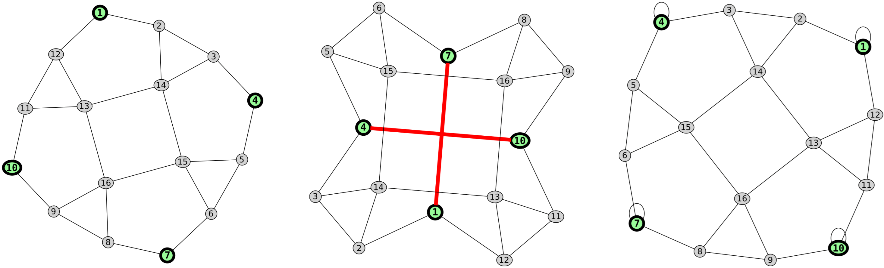
As an example of a decorating graph H, consider the graph of a potentially possible polycyclic molecule in Figure 1. Although we will be only interested in some mathematical manipulations using such a graph, we note briefly and without references that molecules with conditionally planar polycyclic fragments play many roles in nature and synthetic chemistry. Here, we can first recall two important molecules of life that are responsible for supplying living cells with oxygen: chlorophyll for flora and porphyrin for fauna. Other similar molecules are widely used as drugs, dyes, semiconductors, molecular magnets, and monomers to create functional polymers, the latter of which are most closely related to our topic of graph decoration.

The middle graph $H_1$ in Figure 1 with two (red) edges added to the original graph H on the left is a front divisor of any decorated construct in which the contact vertices of any two adjacent copies of H are connected, as corresponds to the endpoints of the highlighted edges of $H_1$. When connecting only the identically labeled vertices of any pair of adjacent copies of H, the front divisor $H_2$ is the graph with loops on the right-hand side of Figure 1. Note that the latter is feasible only in the case of decorating a quasibipartite 4-regular graph G, which in this text is the union of its edge-disjoint 2-factors (2-regular spanning subgraphs), each of which consists of cycles of the same even length, regardless of whether G is a bipartite graph or not. In our example, due to the symmetry of H, differently labeled vertices in pairs $(1, 7)$ and $(4, 10)$ are equivalent in their location in the graph, which allows for a combined case as a variant of decorating the quasibipartite graph G, when graphs $H_1$ and $H_2$ will both simultaneously be frontal divisors of $DG$.

The spectra of the three graphs (obtained with Maple) are as follows:

$$\begin{array}{cc}\hfill \mathrm{Sp}\left(H\right)=& \{3.236067977, {2.342923083}^2, 1.561552813, 1^2, {0.4706834203}^2, {(-1)}^3,\hfill \\ & -1.236067977, -{1.813606504}^2, -2, -2.561552813\};\hfill \\ \hfill \mathrm{Sp}\left(H_1\right)=& \{3.342923083, {2.236067977}^2, 1.732050808, 1.561552813, 1.470683420, 0^2,\hfill \\ & -0.813606504, {(-1)}^3, -1.732050808, -{2.236067977}^2, -2.561552813\}; \hfill \\ \hfill \mathrm{Sp}\left(H_2\right)=& \{3.342923083, {2.561552813}^2,1.732050808, 1.561552813, 1.470683420, 1^2,\hfill \\ & -0.813606504, {(-1)}^3, -{1.561552813}^2, -1.732050808, -2.561552813\}.\hfill \end{array}$$

All these spectra have a subspectrum of five eigenvalues: $\{1.561552813, {(-1)}^3, -2.561552813\}$. Of interest is the presence of 10 common eigenvalues for the front divisors $H_1$ and $H_2$: $\{3.342923083, 1.732050808, 1.561552813, 1.470683420, -0.813606504, {(-1)}^3, -1.732050808, -2.561552813\}$. Thus, the above-discussed scheme of connecting copies of the graph H when decorating any quasibipartite 4-regular graph G allows for a variant with presence in the spectrum of the decorated graph $DG$ of at least $16\times 2=32$ common eigenvalues (with repetitions of some of them), among which there are at least $16\times 2-10=22$ distinct eigenvalues. Specifically, these include $\mathrm{Sp}\left(H_1\right)\cup \mathrm{Sp}\left(H_2\right)=\{3.342923083, {2.561552813}^2, {2.236067977}^2, 1.732050808, 1.561552813, 1.470683420, 1^2, 0^2, -0.813606504, {(-1)}^3, -{1.561552813}^2, -1.732050808, -{2.236067977}^2, -2.561552813\}$ (which plays a role below).

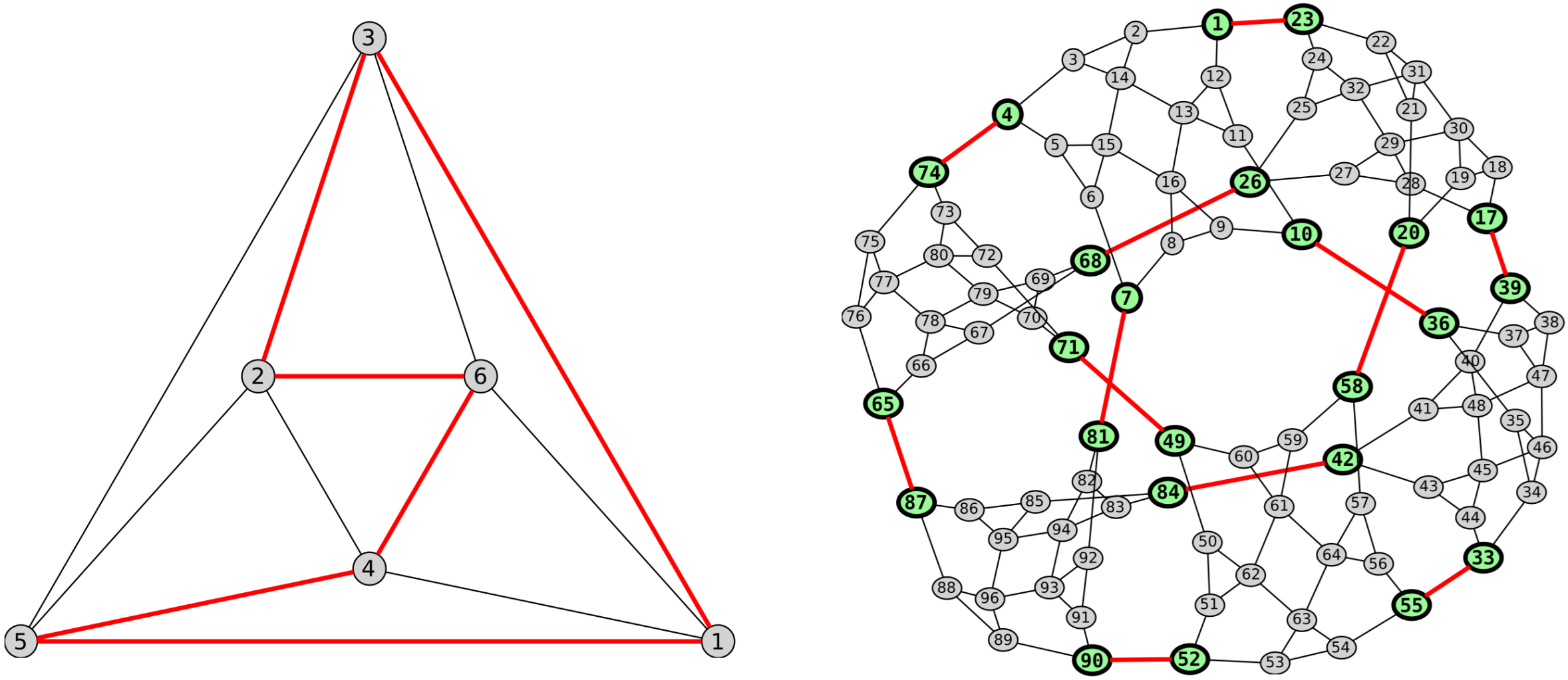
To show how the theory we describe is confirmed in practice, let us consider an example of vertex decoration of the second-smallest quasibipartite 4-regular graph O of the octahedron by the graph H from Figure 1, which results in the graph $HO$ from Figure 2. In passing, we note that the graph O of the octahedron often arises, for example, when considering structural problems of crystallography and the chemistry of coordination compounds, such as $\mathrm{Mo}{\left(\mathrm{CO}\right)}_6,{\left[\mathrm{Co}{\left({\mathrm{NH}}_3\right)}_6\right]}^{3+},{\left[\mathrm{Co}{\left(\mathrm{Cl}\right)}_6\right]}^{3-}$, and many others.

The spectrum of $HO$ is

$$\begin{array}{cc}\hfill & \mathrm{Sp}\left(HO\right)=\{\mathbf{3.342923083}, 2.341924782, {3.270445532}^2, 3.269080177, 3.228713000, 3.225434333,\hfill \\ & {\mathbf{2.561552813}}^{\mathbf{2}}, 2.505938397, {2.495372895}^2, 2.478434161, {2.334955886}^2, 2.329887095,\hfill \\ & {\mathbf{2.236067977}}^{\mathbf{2}}, \mathbf{1.732050808}, {\mathbf{1.561552813}}^{\mathbf{6}}, 1.480460971, \mathbf{1.470683420}, {1.460814387}^2,\hfill \\ & 1.425065119, 1.205249627, {1.180216752}^2,1.165242339, {\mathbf{1}}^{\mathbf{2}},{0.09704550594}^2, 0.6197646484,\hfill \\ & 0.5398257877, 0.4783213042, {0.4022276804}^2, 0.2618692558, 0.1149062658, 0.08795302234,\hfill \\ & {\mathbf{0}}^{\mathbf{2}}, -\mathbf{0.813606504}, {(-\mathbf{1})}^{\mathbf{18}}, -{1.168919470}^2, -1.173630588, -1.334353903, -1.367738905,\hfill \\ & -{\mathbf{1.561552813}}^{\mathbf{2}}, -1.595070783, -{1.614698386}^2, -\mathbf{1.732050808},-2.016356901, -2.068891533,\hfill \\ & -{2.131047156}^2, -2.143501108, -{\mathbf{2.236067977}}^{\mathbf{2}}, -2.318907319, -{2.326413626}^2,\hfill \\ & -2.361632749, -2.377986497, -{\mathbf{2.561552813}}^{\mathbf{6}}\},\hfill \end{array}$$

where the eigenvalues in bold belong to the union $\mathrm{Sp}\left(H_1\right)\cup \mathrm{Sp}\left(H_2\right)$ of the spectra of both divisors $H_1$ and $H_2$ described above, and some of these eigenvalues can be represented in the spectrum of the decorated graph $HO$, even with greater multiplicity than in $\mathrm{Sp}\left(H_1\right)\cup \mathrm{Sp}\left(H_2\right)$. Thus, the theory we are discussing is indeed workable. We only want to remind readers that if the graph G being decorated is not quasibipartite, then the graph $HG$ obtained by its vertex decoration with the graph H is not required to have the graph $H_2$ as its divisor, although there may be a decoration variant in which $HG$ has as its divisor the graph $H_1$. We invite readers to verify this for themselves using the simplest nonquasibipartite 4-regular graph $G=K_5$. By partial analogy with quasibipartite graphs, this graph can be decomposed (in 12 ways) into two edge-disjoint Hamiltonian 5-cycles (which are 2-factors), and the vertices can be decorated according to any pair of such complementary cycles, just as was performed with the Hamiltonian 6-cycles ${\mathrm{Ham}}_1$ and ${\mathrm{Ham}}_2$ of the octahedron above (see description to Figure 2). The resulting graph $H{K}_5$ will have divisor $H_1$, but will not have divisor $H_2$.

Proposition 7 allows us to define the entire class $\Pi$ of $DG$ graphs obtained as stated in its conditions with the same permutation $\varpi$ (matrix $M_{\varpi }$) and the same graph H, with the same labeling of its contact vertices, taking only different r-regular r-edge-colorable graphs G. Thus, all graphs $Q\in \Pi$ have at least $\left|V\right(H\left)\right|$ common eigenvalues belonging to the divisor graph $\Gamma \left(\mathcal{B}\right)$. Graphs that have a common subspectrum of eigenvalues are called subspectral [15,16,17,18,19,20,21,22,23,24], and graphs whose spectra are completely identical are called cospectral or isospectral [9,10,15,25,26,36]. Families of subspectral dendrimers in which the spectrum of each subsequent member completely includes the spectrum of any of its predecessors (taking into account all multiplicities of eigenvalues) are studied in [30]. The problem of cospectrality of graphs from $\Pi$ has been studied only for paraline graphs (recall in a broader context [45,46,47,48,49,50,51,52,53]), which are all included in this class. As follows from $\left(2\right)$ [45], $\forall r\in {\mathbb{N}}_{+}$, two nonisomorphic paraline graphs $K_r{G}_1$ and $K_r{G}_2$ are cospectral if and only if the r-regular graphs $G_1$ and $G_2$ are cospectral.

It should be noted that one can think in advance which (labeled) graph X to choose as a decorating graph (in the role of H) for G in order to obtain a given divisor graph $\Gamma \left(\mathcal{B}\right)$ of the graph $DG$ with the desired spectrum. For example, in [54,55], we considered a decorating graph $X=H$ isomorphic to a cycle $C_4$ of length 4 to obtain a divisor graph $\Gamma \left(\mathcal{B}\right)$ isomorphic to the complete graph $K_4$ (the skeletal graph of a tetrahedron), but the decorating principle was different than in the case of graphs of $\Pi$.

From an applied point of view, it is worth remembering that the second definition of a decorated graph $DG$ is a polymer obtained by ‘polymerization’ of graph H as a ‘monomer’ (according to ‘plan’ G). This acquires real meaning if we keep in mind molecular graphs and talk about what they represent without quotation marks. The chemical process of uniform polymerization with the same method of connecting identical monomer units can be represented at an abstract level, for example, in the same way as the construction of graphs of the set $\Pi$. If we mention in passing nonuniform polymerization (with its graph-theoretical interpretation as above), its product (a ‘copolymer’, if in the case of several different ‘monomers’) can also be compared to a ‘quasicrystal’. In this case, the differently connected monomer units are compared to the different types of environments of atoms by their neighbors in a quasicrystalline lattice. Despite the lack of translational symmetry, a quasicrystal can also have a unit cell defined using equitable partition [92].

In chemistry, it is common practice to synthesize larger molecules using smaller ones as their constituent parts. The diversity of the resulting products is achieved not only due to the different chemical compositions of the initial molecular blocks but also by the way they are connected in the synthesized molecule. This is consistently reflected in the study of topological and other properties of molecular graphs. A good example of this is the series of works [101,102,103,104,105,106,107,108,109], where attention was initially focused on the simplest dimers of the monomeric graph H. Then, in the case of two nonequivalent contact vertices a and b in H, two different dimers can be obtained. One of them, called the S-isomer, connects the identical vertices of two isomorphic copies of H by edges (that is, an a-vertex with an a-vertex and a b-vertex with a b-vertex), while the other, the T-isomer, connects vertices of different sorts (a with b and b with a). The study of $S,T$-isomers served as the beginning of the study of more complex graph constructions with a larger number of not necessarily identical constituent parts and with the use of a larger number of contact vertices in the latter. Using what was said above about the class $\Pi$ graphs, we can make some addition to the study of dimers of isomorphic copies of the graph H under the condition of an arbitrary admissible number $r\ge 2$ of links between two copies of H.

We will need some supporting facts.

Lemma 8.

Let ${}^{2}H$ be the dimer of a labeled graph H obtained by connecting $r\ge 2$ vertices of one isomorphic copy of H via r nonincident edges to the set of the same r vertices of the other copy, according to an involutive permutation ϖ acting on the set of labels of contact vertices. Then, by simultaneously permuting the rows and columns, the adjacency matrix $A\left({}^{2}H\right)$ of ${}^{2}H$ can be reduced to the following $2p\times 2p$ form $(p=|V\left(H\right)\left|\right)$:

$$A\left({}^{2}H\right)=\left[\begin{array}{cc}A\left(H\right)& U_H\\ U_H& A\left(H\right)\end{array}\right],$$

(6)

where $U_H$ is the matrix with the involutive permutation matrix $M_{\varpi }$ as its upper diagonal $r\times r$ block and all other entries being 0s (as above).

Proof. 

$A\left({}^{2}H\right)$ is a $(0,1)$-matrix. The unit $jk$-entry $(j\in \{1, 2, \dots , r\}; k\in \{p+1, p+2, \dots , p+r\left\}\right)$ indicates that the j-th vertex of the first copy of H is connected to the k-th vertex of the second copy. But it is also, in fact, the $(j, k-p)$-th entry of the permutation matrix $M_{\varpi }$. This holds for all unit entries of the same offdiagonal block. Thus, the upper offdiagonal $p\times p$ block of $A\left({}^{2}H\right)$ is indeed equal to $U_H$. Similarly, considering the unit $jk$-entry $(j\in \{p+1, p+2, \dots , p+r\}; k\in \{1, 2, \dots , r\left\}\right)$ of the lower offdiagonal block, we can demonstrate that this block is also equal to $U_H$. Since the nature of both diagonal $p\times p$ blocks is clear, this completes the proof. □

Matrix $\left(6\right)$ has a form convenient enough for its characteristic polynomial to be represented as a product of the characteristic polynomial of the divisor $\mathcal{B}$ of this matrix (defined above and having the same main eigenvalues) and some complementary polynomial of the same power. This is reflected by the following statement:

Proposition 9.

Let $\mathrm{Ch}({}^{2}H;x)$ be the characteristic polynomial of the dimer ${}^{2}H$ of a graph H, as above. Then,

$$\mathrm{Ch}({}^{2}H;x)=\mathrm{Ch}[A\left(H\right)+U_H;x]·\mathrm{Ch}[A\left(H\right)-U_H;x]=\mathrm{Ch}[\mathcal{B}\left(H\right);x]·\mathrm{Ch}[A\left(H\right)-U_H;x],$$

(7)

where $\mathrm{Ch}\left[\mathcal{B}\right(H);x]$ is the characteristic polynomial of the front divisor of the dimer ${}^{2}H$.

Proof. 

For the determinant $det[xI-A\left({}^{2}H\right)]$, the following linear transformations are easy to perform:

$$\begin{array}{c}\hfill \det [x{I}_{2p}-A{}^{2}H)]=\left|\begin{array}{cc}x{I}_p-A\left(H\right)& U_H\\ U_H& x{I}_p-A\left(H\right)\end{array}\right|=\left|\begin{array}{cc}x{I}_p-A\left(H\right)-U_H& U_H\\ U_H-x{I}_p+A\left(H\right)& x{I}_p-A\left(H\right)\end{array}\right|=\\ \hfill \left|\begin{array}{cc}x{I}_p-A\left(H\right)-U_H& U_H\\ O& x{I}_p-A\left(H\right)+U_H\end{array}\right|=\det [x{I}_p-A\left(H\right)-U_H]\det [x{I}_p-A\left(H\right)+U_H]=\\ \hfill \mathrm{Ch}[A\left(H\right)+U_H;x]·\mathrm{Ch}[A\left(H\right)-U_H;x]=\mathrm{Ch}[\mathcal{B}\left(H\right);x]·\mathrm{Ch}[A\left(H\right)-U_H;x],\end{array}$$

(8)

which is the proof. □

By concentrating our attention on the equitable partition of graph vertices (resp. entries of the adjacency matrix), we practically considered polymer graphs constructed from one type of structural unit (in another interpretation, isomorph copies of a graph decorating the vertices of the original graph). However, in the general case, for our purposes it is also possible to construct a larger graph with a given subspectrum from smaller graphs of different types. Here, we are talking about using suitable graph products. From a fairly large arsenal of such operations on graphs, we will consider only two of the most famous and best studied, which, it seems to us, is enough for an interested reader to get an idea of and become acquainted with other such operations (in the context of graph spectra, see [9,10,110]). Here, it should be emphasized that, as follows from the definition of the characteristic polynomial of a graph, spectral graph theory is organically based on matrix theory in its specific application to the adjacency matrices of graphs. Our following examples also serve to confirm what has already been said.

The cardinal, tensor, or Kronecker product $H=H_1\times H_2$ of two graphs, $H_1$ and $H_2$ [110,111,112,113], with the vertex sets $V_1$ and $V_2$, respectively, has $V_1\times V_2$ as its vertex set, and a vertex $u=(u_1,u_2)$ is adjacent to $v=(v_1,v_2)$ in H whenever $u_1\sim v_1$ in $H_1$ and $u_2\sim v_2$ in $H_2$, where ”∼” denotes “adjacent”. The name of the product is due to the fact that the adjacency matrix $A\left(H\right)$ of H is a tensor or Kronecker product $A_1\otimes A_2$ [114,115] of the adjacency matrices $A_1$ and $A_2$ of the graphs $H_1$ and $H_2$, respectively. The operation ⊗ is associative (for the product of three or more matrices), $A_1\otimes A_2\otimes A_3=(A_1\otimes A_2)\otimes A_3=A_1\otimes (A_2\otimes A_3)$, but is not commutative (when $A_1\otimes A_2\ne A_2\otimes A_1$ as it looks like) in general; however, graphs with adjacency matrices $A_1\otimes A_2$ and $A_2\otimes A_1$ are always isomorphic and differ only in the numbering of the vertices: $G_1\times G_2\cong G_2\times G_1$.

We will name some important properties of the tensor product of graphs. First, we present the following combined (of two) theorem [111,113]:

Theorem 10.

The tensor (Kronecker) product $H=H_1\times H_2$ of graphs $H_1$ and $H_2$ is connected if and only if both factors $H_1$ and $H_2$ are connected and at least one is not bipartite. Moreover, if either $H_1$ or $H_2$ is bipartite, then so is their product H; H is regular if both $H_1$ and $H_2$ are regular.

In the context of this work, the following theorem [110] has practical significance:

Theorem 11.

Let $H_1$ and $H_2$ be two graphs on $n_1$ and $n_2$ vertices, respectively. Let ${\lambda }_1,{\lambda }_2,\dots ,{\lambda }_{n_1}$ be the eigenvalues of $H_1$ and ${\mu }_1, {\mu }_2, \dots , {\mu }_{n_2}$ be those of $H_2$ (listed according to multiplicity). Then, the eigenvalues of $H_1\times H_2$ are ${\lambda }_i{\mu }_j$ $(i=1, 2, \dots , n_1; j=1, 2, \dots , n_2)$.

Proof . 

(A known fact [110].) The adjacency matrix $A(H_1\times H_2)$ is the tensor (Kronecker) product of adjacency matrices of $H_1$ and $H_2$, that is, $A(H_1\times H_2)=A\left(H_1\right)\otimes A\left(H_2\right)$ (see [9], p. 67). The statement follows from the common spectral properties of the tensor (Kronecker) product of arbitrary (square) matrices [114,115]. □

We also derive the following corollary, which is particularly important to us:

Corollary 11.1.

Let $H_1$ be a graph with $\mathfrak{m}\left(1\right)\ge 1$ eigenvalues equal to 1. Then, the spectrum of the tensor product $H_1\times H_2$ of $H_1$ and arbitrary graph $H_2$ contains $\mathfrak{p}\ge \mathfrak{m}\left(1\right)$ occurrences of the full spectrum of $H_2$ as a subspectrum (taking into account the multiplicities of the eigenvalues). If $H_2$ is bipartite (and $H_1$ is not), $\mathfrak{p}\ge \mathfrak{m}\left(1\right)+\mathfrak{m}(-1)$, where $\mathfrak{m}(-1)$ is the multiplicity of the eigenvalue $(-1)$ of the graph $H_1$. The tensor product $H_1\times H_2$ can simultaneously include the spectra $H_1$ and $H_2$ if both of the latter consistently satisfy the conditions for separate inclusion of their spectra.

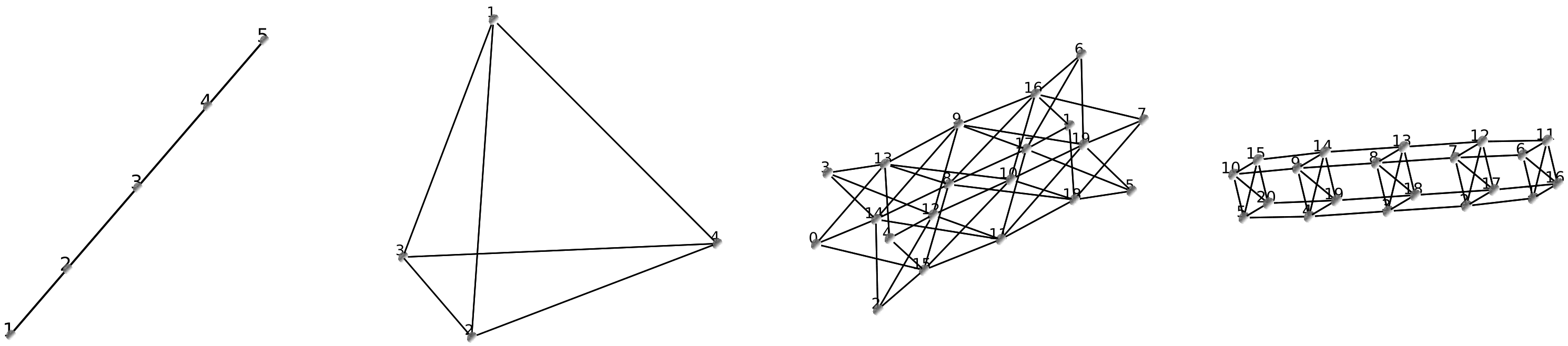
As an example, we perform the described actions with matrices $A\left(P_5\right)={\left[a_{ij}\right]}_{i,j=1}^5$ and $\mathcal{B}=A\left(K_4\right)={\left[b_{kl}\right]}_{kl}^4$ of the path on 5 vertices and the complete graph $K_4$ on 4 vertices, respectively (nonregular graphs also suite us in general). The adjacency matrix of $P_5\times K_4$ (see Figure 3) is

$$A(P_5\times K_4)=\left[\begin{array}{ccccc}O& \mathcal{B}& O& O& O\\ \mathcal{B}& O& \mathcal{B}& O& O\\ O& \mathcal{B}& O& \mathcal{B}& O\\ O& O& \mathcal{B}& O& \mathcal{B}\\ O& O& O& \mathcal{B}& O\end{array}\right]=\left[\begin{array}{cccccccccccccccccccc}0& 0& 0& 0& 0& 1& 1& 1& 0& 0& 0& 0& 0& 0& 0& 0& 0& 0& 0& 0\\ 0& 0& 0& 0& 1& 0& 1& 1& 0& 0& 0& 0& 0& 0& 0& 0& 0& 0& 0& 0\\ 0& 0& 0& 0& 1& 1& 0& 1& 0& 0& 0& 0& 0& 0& 0& 0& 0& 0& 0& 0\\ 0& 0& 0& 0& 1& 1& 1& 0& 0& 0& 0& 0& 0& 0& 0& 0& 0& 0& 0& 0\\ 0& 1& 1& 1& 0& 0& 0& 0& 0& 1& 1& 1& 0& 0& 0& 0& 0& 0& 0& 0\\ 1& 0& 1& 1& 0& 0& 0& 0& 1& 0& 1& 1& 0& 0& 0& 0& 0& 0& 0& 0\\ 1& 1& 0& 1& 0& 0& 0& 0& 1& 1& 0& 1& 0& 0& 0& 0& 0& 0& 0& 0\\ 1& 1& 1& 0& 0& 0& 0& 0& 1& 1& 1& 0& 0& 0& 0& 0& 0& 0& 0& 0\\ 0& 0& 0& 0& 0& 1& 1& 1& 0& 0& 0& 0& 0& 1& 1& 1& 0& 0& 0& 0\\ 0& 0& 0& 0& 1& 0& 1& 1& 0& 0& 0& 0& 1& 0& 1& 1& 0& 0& 0& 0\\ 0& 0& 0& 0& 1& 1& 0& 1& 0& 0& 0& 0& 1& 1& 0& 1& 0& 0& 0& 0\\ 0& 0& 0& 0& 1& 1& 1& 0& 0& 0& 0& 0& 1& 1& 1& 0& 0& 0& 0& 0\\ 0& 0& 0& 0& 0& 0& 0& 0& 0& 1& 1& 1& 0& 0& 0& 0& 0& 1& 1& 1\\ 0& 0& 0& 0& 0& 0& 0& 0& 1& 0& 1& 1& 0& 0& 0& 0& 1& 0& 1& 1\\ 0& 0& 0& 0& 0& 0& 0& 0& 1& 1& 0& 1& 0& 0& 0& 0& 1& 1& 0& 1\\ 0& 0& 0& 0& 0& 0& 0& 0& 1& 1& 1& 0& 0& 0& 0& 0& 1& 1& 1& 0\\ 0& 0& 0& 0& 0& 0& 0& 0& 0& 0& 0& 0& 0& 1& 1& 1& 0& 0& 0& 0\\ 0& 0& 0& 0& 0& 0& 0& 0& 0& 0& 0& 0& 1& 0& 1& 1& 0& 0& 0& 0\\ 0& 0& 0& 0& 0& 0& 0& 0& 0& 0& 0& 0& 1& 1& 0& 1& 0& 0& 0& 0\\ 0& 0& 0& 0& 0& 0& 0& 0& 0& 0& 0& 0& 1& 1& 1& 0& 0& 0& 0& 0\end{array}\right].$$

(9)

The characteristic polynomial $\mathrm{Ch}(P_5\times K_4;x)$ of the graph $P_5\times K_4$ in Figure 3 (or the matrix $A(P_5\times K_4)$ in $\left(9\right)$) is

$$\begin{array}{cc}\hfill & x^{20}-48x^{18}+732x^{16}-5104x^{14}+18918x^{12}-39312x^{10}+45468x^8-27216x^6+6561x^4.\hfill \end{array}$$

The corresponding spectrum is $\mathrm{Sp}(P_5\times K_4)=\{\pm 3\sqrt{3}, \pm 3, {(\pm \sqrt{3})}^3, \pm 1^3, 0^4\}$, where superscripts denote the multiplicities of the eigenvalues. Also, the spectra of $P_5$ and $K_4$ are $\mathrm{Sp}\left(P_5\right)=\{\sqrt{3}, 1, 0, -1, -\sqrt{3}\}$ and $\mathrm{Sp}\left(K_4\right)=\{3, {(-1)}^3\}$. It is easy to check that the spectrum $\mathrm{Sp}(P_5\times K_4)$ consists of all binary products of the eigenvalues of the graphs $P_5$ and $K_4$, as follows from Theorem 11, and contains as subspectra a threefold full spectrum of the graph $P_5$ and a single full spectrum of the graph $K_4$, which is consistent with Corollary 11.1. In the first case, the threefoldness follows from the fact that the graph $P_5$ is bipartite, and the graph $K_4$ has three eigenvalues $(-1)$; in the second case, the onefoldness is explained by the fact that the graph $P_5$ has only one eigenvalue, 1, and the graph $K_4$ is not bipartite. It is necessary to pay attention to the fact that copies of the spectra of $P_5$ and $K_4$ inside the spectrum of $P_5\times H_2$ have three common eigenvalues $(-1)$ in total. Also, it should be noted that the product graph $P_5\times K_4$ is bipartite (and thus all its eigenvalues are represented with both signs ±) because $P_5$ is bipartite (see Theorem 10).

Above, we focused on the topic of equitable partition and graph divisors. It is quite compatible with the topic of graph products. Here, we want to again use our spectral example to illustrate the the usefulness of another corollary we deduced from Theorem 11:

Corollary 11.2.

Let $H_1^{\prime }$ and $H_2^{\prime }$ be arbitrary divisors of graphs $H_1$ and $H_2$, respectively. Then, $H_1^{\prime }\times H_2^{\prime }$ is a divisor of the tensor product $H_1\times H_2$, where all the named graphs are, in general, weighted graphs with weighted adjacency matrices.

The first graph $H_1=P_5$ in Figure 3 allows, due to its symmetry, an equitable partition of its vertex set into orbits $\{1, 5\}$, $\{2, 4\}$, and $\left\{3\right\}$. The corresponding divisor graph $H_1^{\prime }$ has a weighted adjacency matrix

$$W\left(H_1^{\prime }\right)=\left[\begin{array}{ccc}0& 1& 0\\ 1& 0& 1\\ 0& 2& 0\end{array}\right]$$

(10)

with eigenvalues $\{\pm \sqrt{3},0\}$, which indeed all fall into the spectrum of $P_5$ (see above). The minimum-size divisor $H_2^{\prime }$ corresponds to an equitable partition of the second graph $H_2=K_4$, with one orbit $\{1,2,3,4\}$ (where the vertex numbering is related to $H_2$); it has a weighted adjacency matrix $W\left(H_2^{\prime }\right)=\left[3\right]$ with one entry 3 and one eigenvalue 3, which is also an eigenvalue of $H_2=K_4$. A weighted adjacency matrix of $H_1^{\prime }\times H_2^{\prime }$ is

$$W(H_1^{\prime }\times H_2^{\prime })=\left[\begin{array}{ccc}0·\left[3\right]& 1·\left[3\right]& 0·\left[3\right]\\ 1·\left[3\right]& 0·\left[3\right]& 1·\left[3\right]\\ 0·\left[3\right]& 2·\left[3\right]& 0·\left[3\right]\end{array}\right]=\left[\begin{array}{ccc}0& 3& 0\\ 3& 0& 3\\ 0& 6& 0\end{array}\right]$$

(11)

with eigenvalues $\{\pm 3\sqrt{3}, 0\}$, which are all actually included in the spectrum of $H_1\times H_2$. Corollary 11.2 can help in finding divisors of the tensor product of graphs in cases when all graphs involved are large and/or have many divisors. This also applies to equitable partitions of the mentioned graphs.

Figure 3. Original graphs $P_5$ and $K_4$ with their products $P_5\times K_4$ and $P_5$□$K_4$ (from left to right). [Used Maple].

Figure 3. Original graphs $P_5$ and $K_4$ with their products $P_5\times K_4$ and $P_5$□$K_4$ (from left to right). [Used Maple].

The simplest examples of regular tensor (Kronecker) products are 3-regular $H\times K_2$ and 4-regular $C_{n_1}\times C_{n_2}$ products, where H is a nonbipartite cubic graph and at least one of the cycles $C_{n_1}$ and $C_{n_2}$ is odd. Given their low, quite chemical vertex valencies, such regular products may (with homeomorphic realization) turn out to be potential molecular graphs and objects of study in mathematical chemistry [116]. We will not dwell on this issue here, but will move on to considering another graph product.

In graph theory, the Cartesian product $G_1\square G_2$ of graphs $G_1$ and $G_2$ [110,111,112,117,118] is a graph such that the vertex set of $G_1\square G_2$ is the Cartesian product $V\left(G_1\right)\times V\left(G_2\right)$ of their vertex sets $\left(\right|V(G_1|=n_1;|V\left(G_2\right)|=n_2)$; and any two vertices $(u,u^{\prime })$ and $(v,v^{\prime })$ are adjacent in $G_1\square G_2$ if and only if either $u=v$ and $u^{\prime }$ is adjacent with $v^{\prime }$ in $G_2$, or $u^{\prime }=v^{\prime }$ and u is adjacent with v in $G_1$. As in the previous case, this definition can be equivalently expressed in matrix form. The adjacency matrix $A(G_1\square G_2)$ of the Cartesian product $G_1\square G_2$ (see p. 37 in [119]) is

$$A(G_1\square G_2)=A(G_1\otimes I_{n_2}+I_{n_1}\otimes A\left(G_2\right)).$$

(12)

This product is associative and commutative: for any graphs $G_1,G_2,G_3$, $G_1\square G_2\square G_3=(G_1\square G_2)\square G_3=G_1\square (G_2\square G_3)$ and $G_1\square G_2\cong G_2\square G_1$. Similar to the case of the tensor (Kronecker) product, the adjacency matrices $A(G_1\square G_2)$ and $A(G_2\square G_1)$ look different in general, but they represent isomorphic graphs that differ only in the numbering of the vertices. The following statement was proved by Sabidussi ([120], Lemma $2.3$; [117], Corollary $5.2$, p. 41):

Theorem 12.

For the Cartesian product $G=G_1\square G_2$ of graphs $G_1$ and $G_2$, the inequality $\kappa \left(G\right)\ge \kappa \left(G_1\right)+\kappa \left(G_2\right)$ holds, where $\kappa \left(G\right)$ is the vertex connectivity of G. In particular, $G=G_1\square G_2$ is connected if both $G_1$ and $G_2$ are connected.

In our context, the following theorem [110] plays an important practical role:

Theorem 13.

Let $G_1$ and $G_2$ be two graphs on $n_1$ and $n_2$ vertices, respectively. Let ${\lambda }_1,{\lambda }_2,\dots ,{\lambda }_{n_1}$ be the eigenvalues of $G_1$ and ${\mu }_1,{\mu }_2,\dots ,{\mu }_{n_2}$ be those of $G_2$ (listed according to multiplicity). Then, the eigenvalues of $G_1\square G_2$ are ${\lambda }_i+{\mu }_j$$(i=1,2,\dots ,n_1;j=1,2,\dots ,n_2)$.

From Theorem 13, we obtain a corollary directly related to the inclusion of the full spectrum of one of the factors in the spectrum of the product:

Corollary 13.1.

Let $G_1$ be a graph with $\mathfrak{m}\left(0\right)\ge 1$ eigenvalues equal to 0. Then, the spectrum of the Cartesian product $G_1\square G_2$ of $G_1$ and arbitrary graph $G_2$ contains $\mathfrak{p}\ge \mathfrak{m}\left(0\right)$ occurrences of the full spectrum of $G_2$ as a subspectrum (taking into account the multiplicities of the eigenvalues). The Cartesian product $G_1\square G_2$ can simultaneously include the spectra $G_1$ and $G_2$ if both of the latter consistently satisfy the conditions for separate inclusion of their spectra.

As an example, we can explicitly write the adjacency matrix $A(P_3\square K_4)$ of the Cartesian product $P_5\square K_4$ (see Figure 3) according to the R.H.S. of $\left(12\right)$:

$$A(P_5\square K_4)=\left[\begin{array}{cccccccccccccccccccc}0& 0& 0& 0& 1& 0& 0& 0& 0& 0& 0& 0& 0& 0& 0& 0& 0& 0& 0& 0\\ 0& 0& 0& 0& 0& 1& 0& 0& 0& 0& 0& 0& 0& 0& 0& 0& 0& 0& 0& 0\\ 0& 0& 0& 0& 0& 0& 1& 0& 0& 0& 0& 0& 0& 0& 0& 0& 0& 0& 0& 0\\ 0& 0& 0& 0& 0& 0& 0& 1& 0& 0& 0& 0& 0& 0& 0& 0& 0& 0& 0& 0\\ 1& 0& 0& 0& 0& 0& 0& 0& 1& 0& 0& 0& 0& 0& 0& 0& 0& 0& 0& 0\\ 0& 1& 0& 0& 0& 0& 0& 0& 0& 1& 0& 0& 0& 0& 0& 0& 0& 0& 0& 0\\ 0& 0& 1& 0& 0& 0& 0& 0& 0& 0& 1& 0& 0& 0& 0& 0& 0& 0& 0& 0\\ 0& 0& 0& 1& 0& 0& 0& 0& 0& 0& 0& 1& 0& 0& 0& 0& 0& 0& 0& 0\\ 0& 0& 0& 0& 1& 0& 0& 0& 0& 0& 0& 0& 1& 0& 0& 0& 0& 0& 0& 0\\ 0& 0& 0& 0& 0& 1& 0& 0& 0& 0& 0& 0& 0& 1& 0& 0& 0& 0& 0& 0\\ 0& 0& 0& 0& 0& 0& 1& 0& 0& 0& 0& 0& 0& 0& 1& 0& 0& 0& 0& 0\\ 0& 0& 0& 0& 0& 0& 0& 1& 0& 0& 0& 0& 0& 0& 0& 1& 0& 0& 0& 0\\ 0& 0& 0& 0& 0& 0& 0& 0& 1& 0& 0& 0& 0& 0& 0& 0& 1& 0& 0& 0\\ 0& 0& 0& 0& 0& 0& 0& 0& 0& 1& 0& 0& 0& 0& 0& 0& 0& 1& 0& 0\\ 0& 0& 0& 0& 0& 0& 0& 0& 0& 0& 1& 0& 0& 0& 0& 0& 0& 0& 1& 0\\ 0& 0& 0& 0& 0& 0& 0& 0& 0& 0& 0& 1& 0& 0& 0& 0& 0& 0& 0& 1\\ 0& 0& 0& 0& 0& 0& 0& 0& 0& 0& 0& 0& 1& 0& 0& 0& 0& 0& 0& 0\\ 0& 0& 0& 0& 0& 0& 0& 0& 0& 0& 0& 0& 0& 1& 0& 0& 0& 0& 0& 0\\ 0& 0& 0& 0& 0& 0& 0& 0& 0& 0& 0& 0& 0& 0& 1& 0& 0& 0& 0& 0\\ 0& 0& 0& 0& 0& 0& 0& 0& 0& 0& 0& 0& 0& 0& 0& 1& 0& 0& 0& 0\end{array}\right]+\left[\begin{array}{cccccccccccccccccccc}0& 1& 1& 1& 0& 0& 0& 0& 0& 0& 0& 0& 0& 0& 0& 0& 0& 0& 0& 0\\ 1& 0& 1& 1& 0& 0& 0& 0& 0& 0& 0& 0& 0& 0& 0& 0& 0& 0& 0& 0\\ 1& 1& 0& 1& 0& 0& 0& 0& 0& 0& 0& 0& 0& 0& 0& 0& 0& 0& 0& 0\\ 1& 1& 1& 0& 0& 0& 0& 0& 0& 0& 0& 0& 0& 0& 0& 0& 0& 0& 0& 0\\ 0& 0& 0& 0& 0& 1& 1& 1& 0& 0& 0& 0& 0& 0& 0& 0& 0& 0& 0& 0\\ 0& 0& 0& 0& 1& 0& 1& 1& 0& 0& 0& 0& 0& 0& 0& 0& 0& 0& 0& 0\\ 0& 0& 0& 0& 1& 1& 0& 1& 0& 0& 0& 0& 0& 0& 0& 0& 0& 0& 0& 0\\ 0& 0& 0& 0& 1& 1& 1& 0& 0& 0& 0& 0& 0& 0& 0& 0& 0& 0& 0& 0\\ 0& 0& 0& 0& 0& 0& 0& 0& 0& 1& 1& 1& 0& 0& 0& 0& 0& 0& 0& 0\\ 0& 0& 0& 0& 0& 0& 0& 0& 1& 0& 1& 1& 0& 0& 0& 0& 0& 0& 0& 0\\ 0& 0& 0& 0& 0& 0& 0& 0& 1& 1& 0& 1& 0& 0& 0& 0& 0& 0& 0& 0\\ 0& 0& 0& 0& 0& 0& 0& 0& 1& 1& 1& 0& 0& 0& 0& 0& 0& 0& 0& 0\\ 0& 0& 0& 0& 0& 0& 0& 0& 0& 0& 0& 0& 0& 1& 1& 1& 0& 0& 0& 0\\ 0& 0& 0& 0& 0& 0& 0& 0& 0& 0& 0& 0& 1& 0& 1& 1& 0& 0& 0& 0\\ 0& 0& 0& 0& 0& 0& 0& 0& 0& 0& 0& 0& 1& 1& 0& 1& 0& 0& 0& 0\\ 0& 0& 0& 0& 0& 0& 0& 0& 0& 0& 0& 0& 1& 1& 1& 0& 0& 0& 0& 0\\ 0& 0& 0& 0& 0& 0& 0& 0& 0& 0& 0& 0& 0& 0& 0& 0& 0& 1& 1& 1\\ 0& 0& 0& 0& 0& 0& 0& 0& 0& 0& 0& 0& 0& 0& 0& 0& 1& 0& 1& 1\\ 0& 0& 0& 0& 0& 0& 0& 0& 0& 0& 0& 0& 0& 0& 0& 0& 1& 1& 0& 1\\ 0& 0& 0& 0& 0& 0& 0& 0& 0& 0& 0& 0& 0& 0& 0& 0& 1& 1& 1& 0\end{array}\right]$$

(13)

and, finally,

$$A(P_5\square K_4)=\left[\begin{array}{cccccccccccccccccccc}0& 1& 1& 1& 1& 0& 0& 0& 0& 0& 0& 0& 0& 0& 0& 0& 0& 0& 0& 0\\ 1& 0& 1& 1& 0& 1& 0& 0& 0& 0& 0& 0& 0& 0& 0& 0& 0& 0& 0& 0\\ 1& 1& 0& 1& 0& 0& 1& 0& 0& 0& 0& 0& 0& 0& 0& 0& 0& 0& 0& 0\\ 1& 1& 1& 0& 0& 0& 0& 1& 0& 0& 0& 0& 0& 0& 0& 0& 0& 0& 0& 0\\ 1& 0& 0& 0& 0& 1& 1& 1& 1& 0& 0& 0& 0& 0& 0& 0& 0& 0& 0& 0\\ 0& 1& 0& 0& 1& 0& 1& 1& 0& 1& 0& 0& 0& 0& 0& 0& 0& 0& 0& 0\\ 0& 0& 1& 0& 1& 1& 0& 1& 0& 0& 1& 0& 0& 0& 0& 0& 0& 0& 0& 0\\ 0& 0& 0& 1& 1& 1& 1& 0& 0& 0& 0& 1& 0& 0& 0& 0& 0& 0& 0& 0\\ 0& 0& 0& 0& 1& 0& 0& 0& 0& 1& 1& 1& 1& 0& 0& 0& 0& 0& 0& 0\\ 0& 0& 0& 0& 0& 1& 0& 0& 1& 0& 1& 1& 0& 1& 0& 0& 0& 0& 0& 0\\ 0& 0& 0& 0& 0& 0& 1& 0& 1& 1& 0& 1& 0& 0& 1& 0& 0& 0& 0& 0\\ 0& 0& 0& 0& 0& 0& 0& 1& 1& 1& 1& 0& 0& 0& 0& 1& 0& 0& 0& 0\\ 0& 0& 0& 0& 0& 0& 0& 0& 1& 0& 0& 0& 0& 1& 1& 1& 1& 0& 0& 0\\ 0& 0& 0& 0& 0& 0& 0& 0& 0& 1& 0& 0& 1& 0& 1& 1& 0& 1& 0& 0\\ 0& 0& 0& 0& 0& 0& 0& 0& 0& 0& 1& 0& 1& 1& 0& 1& 0& 0& 1& 0\\ 0& 0& 0& 0& 0& 0& 0& 0& 0& 0& 0& 1& 1& 1& 1& 0& 0& 0& 0& 1\\ 0& 0& 0& 0& 0& 0& 0& 0& 0& 0& 0& 0& 1& 0& 0& 0& 0& 1& 1& 1\\ 0& 0& 0& 0& 0& 0& 0& 0& 0& 0& 0& 0& 0& 1& 0& 0& 1& 0& 1& 1\\ 0& 0& 0& 0& 0& 0& 0& 0& 0& 0& 0& 0& 0& 0& 1& 0& 1& 1& 0& 1\\ 0& 0& 0& 0& 0& 0& 0& 0& 0& 0& 0& 0& 0& 0& 0& 1& 1& 1& 1& 0\end{array}\right].$$

(14)

The characteristic polynomial $\mathrm{Ch}(P_5\square K_4;x)$ of the graph $P_5\square K_4$ in Figure 3 (or the matrix $A(P_5\square K_4)$ in $\left(14\right)$) is

$$\begin{array}{c}{x}^{20}-46x^{18}-40x^{17}+789x^{16}+1216x^{15}-5976x^{14}-12576x^{13}+19224x^{12}+54592x^{11}-\hfill \\ 21312x^{10}-107584x^9-2032x^8+102912x^7+14080x^6-48384x^5-5376x^4+9216x^3.\hfill \end{array}$$

The corresponding spectrum is $\mathrm{Sp}(P_5\square K_4)=\left\{\right(\sqrt{3}+3), 4, 3, 2, (-\sqrt{3}+3), {(\sqrt{3}-1)}^3, 0^3, {(-1)}^3, {(-2)}^3, {(-\sqrt{3}-1)}^3\}$, where superscripts denote the multiplicities of the eigenvalues. Also, the spectra of $P_5$ and $K_4$ are $\mathrm{Sp}\left(P_5\right)=\{\sqrt{3}, 1, 0, -1, -\sqrt{3}\}$ and $\mathrm{Sp}\left(K_4\right)=\{3, {(-1)}^3\}$. It is easy to check that the spectrum $\mathrm{Sp}(P_5\square K_4)$ consists of all binary sums of the eigenvalues of the graphs $P_5$ and $K_4$, as follows from Theorem 13, and contains as subspectra a onefold full spectrum of the graph $G_2=K_4$, which is consistent with Corollary 13.1. This follows from the fact that the graph $G_1=P_5$ has a unique eigenvalue 0.

We can also formulate another corollary of Theorem 13, similar to Corollary 11.2:

Corollary 13.2.

Let $G_1^{\prime }$ and $G_2^{\prime }$ be arbitrary divisors of graphs $G_1$ and $G_2$, respectively. Then, $G_1^{\prime }\square G_2^{\prime }$ is a divisor of the tensor product $G_1\square G_2$, where all the named graphs are, in general, weighted graphs with weighted adjacency matrices.

For illustration, we use the same weighted adjacency matrices $W\left(H_1^{\prime }\right)$ and $W\left(H_2^{\prime }\right)$ of the weighted divisors of the graphs $H_1=P_5$ and $H_2=K_4$, respectively, that were used above, after Corollary 11.2. Then, the weighted matrix $W(H_1^{\prime }\square H_2^{\prime })$, taking into account $\left(12\right)$, is calculated as

$$W(H_1^{\prime }\square H_2^{\prime })=\left[\begin{array}{ccc}0·\left[1\right]& 1·\left[1\right]& 0·\left[1\right]\\ 1·\left[1\right]& 0·\left[1\right]& 1·\left[1\right]\\ 0·\left[1\right]& 2·\left[1\right]& 0·\left[1\right]\end{array}\right]+\left[\begin{array}{ccc}1·\left[3\right]& 0·\left[3\right]& 0·\left[3\right]\\ 0·\left[3\right]& 1·\left[3\right]& 0·\left[3\right]\\ 0·\left[3\right]& 0·\left[3\right]& 1·\left[3\right]\end{array}\right]=\left[\begin{array}{ccc}0& 1& 0\\ 1& 0& 1\\ 0& 2& 0\end{array}\right]+\left[\begin{array}{ccc}3& 0& 0\\ 0& 3& 0\\ 0& 0& 3\end{array}\right]=\left[\begin{array}{ccc}3& 1& 0\\ 1& 3& 1\\ 0& 2& 3\end{array}\right]$$

(15)

with the characteristic polynomial $\mathrm{Ch}[W\left(H_1^{\prime }\right)\otimes W\left(H_2^{\prime }\right);x]=x^3-9x^2+24x-18$ and whose spectrum is $\{3,(\sqrt{3}+3),(-\sqrt{3}+3)\}$, which is indeed included in the spectrum of $H_1\square H_2=P_5\square K_4$ or the matrix $A(P_5\square K_4)$ in $\left(14\right)$, and which thus illustrates Corollary 13.2.

As for the nonspectral properties of the Cartesian product of graphs, this is described in detail in a special monograph [117] and, of course, in subsequent publications. Among simpler products, $G_1\square G_2$ are skeletal graphs $C_p\square K_2$ of prisms and $C_p\square C_q$$(p,q\ge 3)$ of tori, which are objects of particular interest to specialists in (mathematical) chemistry.

The topic of graph products is combined with the topics of vertex decoration and the equitable partition of graphs with the corresponding divisors. Adjacency matrices of products have a clearly distinguishable structure of partitioning into square blocks. We can conditionally say that these are decorated matrices, where decoration can be understood as inserting the mentioned blocks instead of the entries of the matrix of one of the factors. This same block partition allows replacing blocks in the opposite direction, implementing an equitable partition of adjacency matrices; such a partition is generally not unique and can generate several divisors.

One can take any adjacency $(0,1)$ matrix $A={\left[a_{kl}\right]}_{k,l=1}^n$ of a simple graph G and arbitrarily replace its unit entries with any positive integers while maintaining the symmetry of the matrix, resulting in the matrix $\mathcal{B}={\left[b_{kl}\right]}_{k,l=1}^n$. Having chosen an appropriate common dimension p of the inserted square matrices, insert an arbitrary $p\times p$ $(0, 1)$-block with the same row sums ${\rho }_{{\mathcal{B}}_{kl}}$ equal to the replaced entry $b_{kl}$ in the weighted matrix $\mathcal{B}$. This results in a $pn\times pn$ matrix M of the derived (di)graph whose divisor is the weighted matrix $\mathcal{B}$. There is any countable set of derived (di)graphs on $pn$$(p\in \mathbb{N})$ vertices with a common divisor $\mathcal{B}$. The obtained symmetric matrices M will be adjacency matrices of undirected graphs. This allows us to obtain a countably infinite set of graphs with a common spectrum of the divisor matrix $\mathcal{B}$. Here, recall for example that the matrices on the last sides of $\left(11\right)$ and $\left(15\right)$ are divisors of the matrices on the last sides of $\left(9\right)$ and $\left(14\right)$, respectively. However, they are not symmetric matrices and therefore cannot be used in the role of $\mathcal{B}$ to derive undirected graphs as described above, although both are suitable for constructing directed graphs (possibly with loops).

In general, the tensor and Cartesian products of the same pair of graphs are not isomorphic, but there is a case when they are isomorphic. This is the case of $C_3\times C_3\cong C_3\square C_3$ with characteristic polynomial $x^9-18x^7-12x^6+81x^5+36x^4-168x^3+144x-64$ and spectrum $\{4, 1^4, {(-2)}^4\}$. The 4-regular graph $C_3^{2_{\square }}$ corresponding to these equivalent products can be embedded in the torus as a graph with quadrilateral (rectangular) faces. It can be viewed as the skeletal graph of the ring obtained by gluing three (flexible) triangular prisms at their bases.

The graph $C_3^{2_{\square }}$ and the entire series of toroidal graphs $C_p\square C_q$$(p,q\ge 3)$ are of interest in mathematical chemistry as templates for new molecules (see [54,55]). Here, we deliberately did not immediately call them potential molecular graphs, meaning molecules isomorphic to them. On the one hand, this is because the existence of such molecules cannot be guaranteed in advance; but on the other hand, toroidal graphs are certainly a promising starting material for constructing derivative graphs of potentially synthesized molecules [54,55]. There are at least two approaches to solving such a design problem. First, inventors of new molecules can consider as potential molecular graphs ones homeomorphic to Cartesian products of cycles; see general graph theory in [36] and, in particular, [9,10,38,39] for graph spectra and [116] (with bibl.) for chemical applications. Secondly, one can consider all possible variants of vertex and/or edge decoration of graphs, particularly what we previously started to do in the case of their vertex quadrangulation [54,55] and now continue to discuss in the more general case of any vertex decoration in this paper.

Among other possible methods for determining the common subspectrum of graphs, we would like to mention determining select eigenvalues by embedding, which has found particularly successful application in the work of Dias [18]. This method is not directly related to the equitable partition of graph vertices discussed above, but (when possible) allows finding more general divisors in it that are not front divisors (as above). This more general type of graph divisor is characterized by the absence of a common maximum eigenvalue with the original graph, and the absence of other common main eigenvalues is also possible. All characterization is limited only by the fact that the characteristic polynomial $\mathrm{Ch}(\mathfrak{D};x)$ of the divisor $\mathfrak{D}$ divides the characteristic polynomial $\mathrm{Ch}(G;x)$ of the original graph G. In the context we are describing, $\mathfrak{D}$ is a proper edge subgraph of G$\left(V\right(\mathfrak{D})=V(G);E(\mathfrak{D})\subset E(G\left)\right)$; that is, $\mathfrak{D}$ is also an undirected unweighted subgraph of G (possibly disconnected), while the front divisor $\Gamma \left(\mathcal{B}\right)$ is, in general, a weighted oriented graph (thus, in general, $\Gamma \left(\mathcal{B}\right)⊈G$). Here, we need to move on to reasoning related to eigenvectors.

Let $A={\left[a_{kl}\right]}_{k,l=1}^n$ be the adjacency matrix of a simple graph G with their common eigenvalue spectrum $\{{\lambda }_1, {\lambda }_2, \dots , {\lambda }_n\}$. Also, let ${\mathfrak{v}}_j={(s_{1j}, s_{2j} \dots , s_{nj})}^{\top }$ be the eigenvector corresponding to the eigenvalue ${\lambda }_j$ of the matrix $A\left(G\right)$; $j\in \{1, 2, \dots , n\}$. In general, there is a subset $\mathfrak{S}\subset \{1, 2, \dots , n\}$ of indices (marking the vertices or vertices themselves) for which the corresponding entries of the eigenvector ${\mathfrak{v}}_j$ are equal to zero: $\forall i\in \mathfrak{S}$, $s_{ij}=0$. What does this entail? Let matrix $A^{\prime }$ be the matrix obtained by replacing with zeros all (unit) entries $a_{kl}$ of matrix A for $k, l\in \mathfrak{S}$ (that is, all entries of $A^{\prime }$ in k-th and l-th rows and columns are equal to 0; $k,l\in \mathfrak{S}$). The matrix $A^{\prime }$ is the adjacency matrix of the induced disconnected edge subgraph $G^{\prime }$ of the graph G$(G^{\prime }\subset G)$, in which the vertices corresponding to the zero rows and columns of the matrix $A^{\prime }$ are isolated vertices. In this case, obviously,

$$A^{\prime }{\mathfrak{v}}_j=A^{\prime }\left[\begin{array}{c}{s}_{1j}\\ s_{2j}\\ ⋮\\ s_{nj}\end{array}\right]=A\left[\begin{array}{c}{s}_{1j}\\ s_{2j}\\ ⋮\\ s_{nj}\end{array}\right]=\left[\begin{array}{c}{\lambda }_j{s}_{1j}\\ {\lambda }_j{s}_{2j}\\ ⋮\\ {\lambda }_j{s}_{nj}\end{array}\right]={\lambda }_j{\mathfrak{v}}_j,$$

(16)

that is, ${\lambda }_j$ is simultaneously an eigenvalue of both matrices $A^{\prime }$ and A, as well as of the subgraph $G^{\prime \prime }$ obtained by removing all $\left|\mathfrak{S}\right|$ isolated “zero” vertices from $G^{\prime }$ (or “zero” vertices from G).

As a simple example, consider the eigenvectors of the cycle $C_6$ (benzene graph); see Figure 4.

The motivation for this choice of “zero” vertices is the following column eigenvectors of the cycle $C_6$ (calculated by Maple):

$$\left[\begin{array}{c}2\\ 1\\ 1\\ -1\\ -1\\ -2\end{array}\right], \left[\begin{array}{cccccc}1& -1& 1& -1& -1& -1\\ 1& -1& 0& 1& 0& 1\\ 1& 0& -1& 0& 1& -1\\ 1& 1& -1& -1& -1& 1\\ 1& 1& 0& 1& 0& -1\\ 1& 0& 1& 0& 1& 1\end{array}\right].$$

(17)

On the right-hand side of $\left(17\right)$, the third and fifth column vectors have zero entries in the second and fifth rows, which implies that vertices 2 and 5 are “zero” vertices $(\mathfrak{S}=\{2, 5\left\}\right)$. Alternatively, one can also notice that both the second and fourth column vectors have common zeros in the third and sixth positions from the top $(\mathfrak{S}=\{3, 6\left\}\right)$.

From Figure 4, it follows that the embedding graph $G^{\prime \prime }$ (G less “zero” vertices) consists of two disjoint edges $(1, 6)$ and $(3, 4)$, the total spectrum of which is $\{1^2, {(-1)}^2\}$ and is entirely contained in the spectrum $\{2, 1^2, {(-1)}^2, (-2)\}$ of the cycle $C_6$. Figure 4, chosen as an example, demonstrates a ready-made solution to the problem of partial covering of the original graph $C_6$ by graph divisors of general type (in this case, by two copies of the graph $K_2$) or, in other words, embedding the mentioned copies of the graph $K_2$. But we found the divisors on the basis of already known eigenvectors, whereas the method of embedding was invented precisely for finding divisors (when they exist) without a full spectral solution, based on the structure of the graph under consideration. This method itself is discussed in detail in the mentioned book by Dias [18]. Our goal here was simply to show that there are also graph divisors of the general type whose discovery is not related to either the use of symmetry or more general considerations of equitable partition.

Chemists and physicists constantly need quantum-mechanical calculations of the properties of molecules and solids. There is a fundamental theory that allows one to describe these properties accurately at an abstract level. However, when it comes to precise numerical (ab initio) calculations, they can only be performed for relatively simple molecules with a small number of valence electrons. Approximate methods come to the rescue, the most accessible of which (although not the most accurate) is the simple method of linear combination of atomic orbitals (LCAO) from Hückel (see [18,121,122,123,124]). Because of its simplicity, the Hückel method has proven itself in terms of calculating conjugated $\pi$-electron systems, in which it is generally assumed that each atom contributes one electron to the overall electron system. An example is benzoaromatic hydrocarbons [18,19]. The energy of the electron level in such a system is calculated using the Hückel method as ${\epsilon }_j=\alpha +{\lambda }_j\beta$. Here, $\alpha$ is the Coulomb integral (estimating the energy of the corresponding electron being removed from the atom), $\beta$ is the resonance integral (which determines the strength of interaction between two chemically bonded atoms), and ${\lambda }_j$, with its notation already familiar to us, is the j-th eigenvalue of the corresponding molecular graph (in which the vertices represent atoms and the edges represent chemical bonds between them) [18,121,122,123,124]. Note that $\alpha <0$ and $\beta <0$; therefore, the ground-state level with the minimum electron energy corresponds to the maximum eigenvalue of the molecular graph, while the energy of the upper excited electron level corresponds to the minimum (negative) eigenvalue of this graph. Add that, usually, when the Coulomb integral is conditionally equated to zero, not the absolute energy of the molecule is considered but the energy of its formation from the initial atoms. As a result, the energy levels of the molecule are described only by a constant resonance integral and, as the only dynamic parameter, the corresponding eigenvalue of the molecular graph, that is, as ${\epsilon }_j={\lambda }_j\beta$. Here, it becomes clear why the topic we have outlined is important in quantum chemistry.

The spectral properties of vertex-decorated (regular) graphs of a fairly general type discussed above contribute, in particular, to the development of methods for solving Hückel problems using noncomputer-oriented manual methods. As formulated in [40], such methods allow calculations that “are performed by back-of-the-envelope calculation, bypassing any diagonalization step, even within Hückel theory”. Examples of this can be found in [15,16,17,18,19,20,21,22,23,24]. Note that [24] places special emphasis on degenerate eigenvalues of graphs (with local symmetries), while [125] specifically treats the zero eigenvalue. The structural origin of specific eigenvalues $(\pm 1,\pm 2,\pm \sqrt{2},\pm \sqrt{3},0)$ in graphs of planar molecules was investigated by Dias [126]. Separate attention to eigenvalue $+1$ was given by Randić, El-Basil, and King [127]. See also the paper [39] by Fowler and Rogers and that by Rosenfeld [54], which presents a new result concerning perfect star packing in regular graphs related to the eigenvalue $-1$. Some other structural aspects of the eigenvalues $\pm 1$ were also studied in [54,55]. In a broader context (not just in connection with the application in Hückel’s method), more examples can be found in the books by Cvetković, Doob, and Sachs [9] and Cvetković, Doob, Gutman, and Torgašev [10]. Two books by Cvetković, Rowlinson, and Simić [128,129] describe other cases of graphs having definite eigenvalues; in particular, their second book is specially devoted to graphs with minimal eigenvalue $-2$.

The classical general definition of the rooted product $G\left(H\right)$ of graphs, which was mentioned at the beginning [28,29,30,31,32,33,34,35], in principle, allows for the possibility of decorating the core graph G with different rooted graphs $H_i$ $(i=1, 2,\dots , n=|V\left(G\right)\left|\right)$. However, to our knowledge, this possibility has been used very limitedly by authors in the field of spectral graph theory. For example, in [31], the independent decoration of two parts of a bipartite graph with rooted graphs of two different types was considered. As before, keeping in mind the spectral aspects, we will show below that several alternative ways of decorating an arbitrary subset of the vertices of the graph G with graphs $H_i$ of different types have long been considered. To do this, we will need to use some known facts, particularly the following [9,130]:

Theorem 14.

(Heilbronner [130]). Let Γ be the graph obtained by joining a vertex u of a graph G to a vertex v of a graph H by an edge. Let $G-u(H-v)$ be the induced subgraph of $G\left(H\right)$ obtained by deleting the vertex $u\left(v\right)$ from $G\left(H\right)$. Then,

$$\mathrm{Ch}(\Gamma ;x)=\mathrm{Ch}(G;x)\mathrm{Ch}(H;x)-\mathrm{Ch}(G-u;x)\mathrm{Ch}(H-v;x).$$

(18)

Note that the graph $\Gamma$ from Theorem 14 is essentially the simplest example of a rooted product with a single graph H connected with an edge to the core G. However, Heilbronner’s theorem serves as a starting point for deriving a formula for a more complicated rooted product $G\left(\mathcal{H}\right)$, possibly with a family $\mathcal{H}=\{H_1, H_2, \dots , H_r\}$ of different rooted graphs connected via an edge and with a not necessarily fully utilized core.

Let $N_r$ denote the set $\{0,1,2,\dots ,r\}$, and let $G-V_{\sigma }$$(\sigma \subset N_r)$ denote the graph G less the subset $V_{\sigma }$ of all its vertices $u_k$, whose indices k belong to the subset $\sigma \subseteq N_r$; in particular, $V_{\varnothing }:=\varnothing$. Repeated use of Theorem 14 leads to the corresponding more general result:

Theorem 15.

Let $\Gamma =G\left(\mathcal{H}\right)$ be the rooted product of the core graph G and the family $\mathcal{H}=\{H_1, H_2, \dots , H_r\}$ of $r\le \left|V\right(G\left)\right|$ graphs obtained by connecting by an edge the root $v_j$ of $H_j$ with the vertex $u_j$ of G $(j=1, 2, \dots , r)$. Then, the characteristic polynomial of Γ is

$$\begin{array}{c}\hfill \mathrm{Ch}(\Gamma ;x)=\prod _{j\in N_r\setminus 0}\mathrm{Ch}(H_j;x)\sum _{\forall \sigma \subset N_r}{(-1)}^{\left|\sigma \right|}\mathrm{Ch}(G-V_{\sigma };x)\prod _{j\in \sigma }{\displaystyle \frac{\mathrm{Ch}(H_j-v_j;x)}{\mathrm{Ch}(H_j;x)}}\\ \hfill (N_r=\{1, 2, \dots , r\};{(-1)}^{|V_{\varnothing }|}:=1;\mathrm{Ch}(G-V_{\varnothing };x)\equiv \mathrm{Ch}(G;x);\mathrm{Ch}[G-V\left(G\right);x]:=1).\end{array}$$

(19)

Since the characteristic polynomial (eigenvalue spectrum) of a graph is the characteristic polynomial (spectrum) of its matrix, we can adapt to this particular case the well-known Cauchy’s interlacing theorem for the eigenvalues of Hermitian matrices; see [131,132] and Theorem 4.3.17, p. 242 in [133]):

Theorem 16.

Let $A\left(H\right)$ and $A(H-v)$ be the adjacency matrices of graphs H and $H-v$ above, with the spectra of eigenvalues $\mathrm{Sp}\left(H\right)=\{{\lambda }_1, {\lambda }_2, \dots , {\lambda }_{\left|V\right(H\left)\right|}\}$ and $\mathrm{Sp}(H-v)=\{{\mu }_1, {\mu }_2, \dots , {\mu }_{\left|V\right(H\left)\right|-1}\}$, respectively. Then,

$${\lambda }_j\ge {\mu }_j\ge {\lambda }_{j+1}(j=1, 2, \dots , |V\left(H\right)|-1).$$

(20)

For us, the following obvious corollary of the last theorem is important:

Corollary 16.1.

Let ${\lambda }_j, {\lambda }_{j+1}, \dots , {\lambda }_{j+s-1}$ be $s\ge 1$ consecutive eigenvalues of $A\left(H\right)$ in nonincreasing order $(j+s-1=1, 2, \dots , |V\left(H\right)\left|\right)$. If ${\lambda }_j={\lambda }_{j+1}=\cdots ={\lambda }_{j+s-1}=\alpha$, then ${\mu }_j={\mu }_{j+1}=\cdots ={\mu }_{j+s-2}=\alpha$, where ${\mu }_j, {\mu }_{j+1}, \dots , {\mu }_{j+s-2}$ are consecutive eigenvalues of $A(H-v)$.

Corollary 16.1 can be reinterpreted in graph-theoretical terms with additional consideration of the multiplicities of the eigenvalues:

Corollary 16.2.

Let a graph H have a degenerated eigenvalue α of multiplicity $s\ge 2$. Then, its induced subgraph $H-v$ also has an eigenvalue α of multiplicity t satisfying the two-sided inequality $s-1\le t\le s+1$.

Proof. 

All we need to prove is that $s-1\le t\le s+1$. Let ${\lambda }_j={\lambda }_{j+1}=\cdots ={\lambda }_{j+s-1}=\alpha$, while ${\lambda }_{j-1}\ne \alpha$ and ${\lambda }_{j+s}\ne \alpha$ are as in Corollary 16.1. Given the nonstrictness of interlacing Cauchy’s inequalities $\left(19\right)$, there are only four possible cases:

(1)

${\mu }_{j-1}>{\lambda }_j$ and ${\lambda }_{j+s-1}>{\mu }_{j+s-1}$;

(2)

${\mu }_{j-1}>{\lambda }_j$ and ${\lambda }_{j+s-1}={\mu }_{j+s-1}$;

(3)

${\mu }_{j-1}={\lambda }_j$ and ${\lambda }_{j+s-1}>{\mu }_{j+s-1}$;

(4)

${\mu }_{j-1}={\lambda }_j$ and ${\lambda }_{j+s-1}={\mu }_{j+s-1}$.

• Obviously, in the first case the only $\mu$-eigenvalues equal to $\alpha$ are those that are inside the interval $[{\lambda }_j, \dots , {\lambda }_{j+s-1}]$ of s $\lambda$-values; this gives the lower bound $t=s-1$ (this bound will also be true if we additionally consider the case $s=1$, which is not taken into account by the Corollary 16.2). In the second and third cases, another $\mu$-eigenvalue outside this interval is also equal to $\alpha$, which gives a median value $t=s$. In the final case, two $\mu$-eigenvalues equal to $\alpha$ are added to $s-1$ of the first case, which gives the upper bound $t=s+1$. This completes the proof. □

As an illustration for Corollary 16.2, consider a symmetric tree on seven vertices (the hydrogen-depleted molecular graph of 3-ethyl-n-pentane) that has a double eigenvalue $\pm 1$ $(s=2)$. For H and its three nonisomorphic subgraphs with one vertex deleted, $H-v$, we have

$$\begin{array}{c}•-•-•{<}_{•-•}^{•-•}\{2, {\mathbf{1}}^2, 0, {(-\mathbf{1})}^2, -2\}\mathrm{with}s=s_{\pm 1}=2;\hfill \\ •-•{<}_{•-•}^{•-•}\left\{\sqrt{2+\sqrt{3}}, \mathbf{1}, \sqrt{2-\sqrt{3}}, -\sqrt{2-\sqrt{3}}, -\mathbf{1}, -\sqrt{2+\sqrt{3}}\right\}\mathrm{with}t=s-1=1;\hfill \\ ••{<}_{•-•}^{•-•}\{\sqrt{3}, \mathbf{1}, 0^2, -\mathbf{1}, -\sqrt{3}\}\mathrm{with}t=s-1=1;\hfill \\ {•-•}_{•-•}^{•-•}\{{\mathbf{1}}^3, {(-\mathbf{1})}^3\}\mathrm{with}t=s+1=3.\hfill \end{array}$$

Combining Theorem 14 of Heilbronner and Corollary 16.2 allows us to formulate their common corollary:

Corollary 16.3. 

Let Γ be the graph obtained by joining an arbitrary vertex u of a graph G to an arbitrary vertex v of a graph H by an edge. If H has an eigenvalue α of multiplicity $s\ge 2$, then Γ has the eigenvalue α of multiplicity $t\ge s-1$.

The following theorem seems to be very useful for constructing restricted rooted products with a given subspectrum.

Theorem 17.

Let $\Gamma =G\left(\mathcal{H}\right)$ be the rooted product of the core graph G and the family $\mathcal{H}=\{H_1, H_2, \dots , H_r\}$ of $r\le \left|V\right(G\left)\right|$ graphs obtained by connecting by an edge the root $v_j$ of $H_j$ with the vertex $u_j$ of G $(j=1, 2, \dots , r)$. If $H_j$ has an eigenvalue α of multiplicity $s_j\ge 2$$(j=1, 2, \dots , r)$, then Γ has $t\ge {\sum }_{j=1}^r(s_j-1)$ eigenvalues α. The upper bound for t is at least ${\sum }_{j=1}^r(s_j+1)$ and depends on G and the choice of r contact vertices in it.

Proof. 

First, we note that each term in the full expansion of the right-hand side of $\left(19\right)$ as a sum of terms contains as its factor either $\mathrm{Ch}(H_j;x)$ or $\mathrm{Ch}(H_j-v_j;x)$ $(j=1, 2, \dots , r)$. By virtue of Corollary 16.2, each of the mentioned terms is thus divisible by the factor ${(x-\alpha )}^t$, where $t\ge {\sum }_{j=1}^r(s_j-1)$. It is obvious that, according to Corollary 16.2, a possible upper bound on the value of t is at least ${\sum }_{j=1}^r(s_j+1)$; however, in general, additional eigenvalues equal to $\alpha$ may appear due to the participation of the characteristic polynomials $\mathrm{Ch}(G-V_{\sigma };x)$ in $\left(19\right)$. This completes the proof. □

Since Theorem 17 can be applied to several different eigenvalues in parallel, as was done with a single value of $\alpha$, we can ensure the existence of a graph $\Gamma$ with a given subspectrum by preselecting a family $\mathcal{H}=\{H_1,H_2,\dots ,H_r\}$ of rooted graphs. For example, if we need the eigenvalues $+1$ and $-1$, we can include in $\mathcal{H}$ the seven-vertex tree (hydrogen-depleted molecular graph of 3-ethyl-n-pentane) from our last example. A valuable feature of Theorem 17 is that it is valid for any choice of both r contact vertices in graph G and root vertices in graphs $H_j$ of $\mathcal{H}$, whereas the results we have previously considered generally depend significantly on the connection options of the decorating graphs. Also, ideologically close to Theorem 17 are results that we will consider separately in the next section.

4. Subsequent Results

Consider a couple of more specific cases. Let w be an isolated vertex, $\mathcal{H}=\{H_1, H_2, \dots , H_b\}$ be a family of disjoint connected graphs, and $u_j\in V\left(H_j\right)$ $(j=1, 2, \dots , b)$, then the bridge coalescence graph $K_1·\mathcal{H}$ [134] is obtained from the graphs of $\mathcal{H}$ by adding new edges $w{u}_j$$(j=1, 2, \dots , b)$. The characteristic polynomial $\mathrm{Ch}(K_1·\mathcal{H};x)$ of $K_1·\mathcal{H}$ could be calculated by repeatedly applying Theorem 14 (of Heilbronner), which was already done in Theorem 2.5 of [134]. Since we are only interested in the special case where all graphs $H_j$ in the family $\mathcal{H}$ are isomorphic, we present here only Proposition 2.6 from [134]:

Proposition 18.

Let all graphs $H_1,H_2,\dots ,H_b$ in $\mathcal{H}$ be isomorphic to H, then the characteristic polynomial of the b-tuple bridge coalescence graph $K_1·\mathcal{H}$ is given by

$$\mathrm{Ch}(K_1·\mathcal{H};x)=x{\left[\mathrm{Ch}(H;x)\right]}^b-b\mathrm{Ch}(H-u;x){\left[\mathrm{Ch}(H;x)\right]}^{b-1}(b\ge 2),$$

(21)

where u is a contact vertex of H.

The following corollary (derived using the R.H.S. of $\left(21\right)$) is important for us:

Corollary 18.1.

Let all graphs $H_1,H_2,\dots ,H_b$ in $\mathcal{H}$ be isomorphic to H, then the characteristic polynomial $\mathrm{Ch}(K_1·\mathcal{H};x)$ of the b-tuple $(b\ge 2)$ bridge coalescence graph $K_1·\mathcal{H}$ is divisible by ${\left[\mathrm{Ch}(H;x)\right]}^{b-1}$. In other words, the spectrum $\mathrm{Sp}(K_1·\mathcal{H})$ of $K_1·\mathcal{H}$ contains at least $(b-1)$ times the full spectrum $\mathrm{Sp}\left(H\right)$ of H.

Let $H^{\prime }=K_1·\mathcal{H}$ and $\mathcal{H}$ be a multiset of b isomorph copies of $H^{\prime }$. We want to go a little further and use the entire bridge coalescence graph $K_1·\mathcal{H}$ as a decorating graph with contact vertex w instead of graph H when forming an (incomplete) rooted product $G\left({\mathcal{H}}^{\prime }\right)$ by a via-edge attachment of graphs of ${\mathcal{H}}^{\prime }$ to an arbitrary core graph G. For the simplest case of ${\mathcal{H}}^{\prime }=\left\{H^{\prime }\right\}$, the combined use of Theorem 14 and Corollary 18.1 allows us to formulate the following lemma:

Lemma 19.

Let $\mathcal{H}$ be a family of $b\ge 2$ isomorphic copies of a connected graph H, and let $H^{\prime }=K_1·\mathcal{H}$ be the b-tuple bridge coalescence graph as above. Moreover, let a contact vertex w of $K_1·\mathcal{H}$ be attached via an edge to an arbitrary vertex of an arbitrary connected graph G. Then,

$$\begin{array}{c}\mathrm{Ch}(\Gamma ;x)=\mathrm{Ch}(G;x)\mathrm{Ch}(K_1·\mathcal{H};x)-\mathrm{Ch}(G-u;x)\mathrm{Ch}[(K_1·\mathcal{H})-w;x]=\hfill \\ \mathrm{Ch}(G;x)\mathrm{Ch}(K_1·\mathcal{H};x)-\mathrm{Ch}(G-u;x){\left[\mathrm{Ch}(H;x)\right]}^b=P\left(x\right){\left[\mathrm{Ch}(H;x)\right]}^{b-1}(b\ge 2),\hfill \end{array}$$

(22)

where $P\left(x\right)$ is a polynomial in x whose roots do not necessarily contain any roots of the characteristic polynomial $\mathrm{Ch}(H;x)$. In other words, the spectrum of Γ contains at least $(b-1)$ times the full spectrum $\mathrm{Sp}\left(H\right)$ of H.

Proof. 

By virtue of Corollary 18.1, the first product on the third side of $\left(22\right)$ is divisible by ${\left[\mathrm{Ch}(H;x)\right]}^{b-1}$ and the second product on the third side is divisible by ${\left[\mathrm{Ch}(H;x)\right]}^b$, which means that the entire third side is divisible by ${\left[\mathrm{Ch}(H;x)\right]}^{b-1}$. This is the proof. (In slightly different terms, the equality of the first and last sides of $\left(22\right)$ was also proven in Lemma 11 of [30]). □

As noted above, Lemma 19 is formulated using Heilbronner’s theorem for the characteristic polynomial of a pair of graphs connected by an edge (the case of $G\left({\mathcal{H}}^{\prime }\right)$, when ${\mathcal{H}}^{\prime }=\left\{H^{\prime }\right\}$). In the same way, the result can be obtained step by step for the more general case when the family ${\mathcal{H}}^{\prime }$ contains an arbitrary number of isomorphic copies of $H^{\prime }$. To solve such a problem, one can also use the symmetry of the graphs under consideration. The graph $H^{\prime }=K_1·\mathcal{H}$ can be symbolically represented as a propeller with b blades sharing a common center point. For us, it is enough to see that our propeller has a b-fold symmetry axis (although there may also be other elements of symmetry). The formulae for the characteristic polynomial of a (molecular) graph with b-fold $(b\ge 2)$ symmetry axis are well known (see [30,135,136,137,138,139,140,141]); in particular, Lemma 11 of [30] presents the result in a form equivalent to the last side of $\left(22\right)$.

Lemma 19 considers attaching a single copy of $H^{\prime }$ to the core graph G via an edge; in the general case, when the number of similarly joined copies of $H^{\prime }$ is $r\ge 1$, we can formulate a more general statement for the resulting graph ${\Gamma }^{\prime }$, which is also a corollary of Theorem 15:

Proposition 20.

Let ${\mathcal{H}}^{\prime }=\{H_1^{\prime }, H_2^{\prime }, \dots , H_r^{\prime }\}$ be a multiset of $r\ge 1$ isomorph copies $H_j^{\prime }$ of the b-tuple bridge coalescence graph $H^{\prime }=K_1·H$ as above. Moreover, let a contact vertex $w_j$ of each copy $H_j^{\prime }$ be connected with an edge to an arbitrary vertex $v_j$ of an arbitrary connected graph G; $j=1, 2, \dots , r$. Then, the characteristic polynomial of the resulting graph ${\Gamma }^{\prime }=G·{\mathcal{H}}^{\prime }$ is

$$\begin{array}{c}\hfill \mathrm{Ch}({\Gamma }^{\prime };x)=\sum _{\forall \sigma \subset N_r}{(-1)}^{\left|\sigma \right|}\mathrm{Ch}(G-V_{\sigma };x){\left[\mathrm{Ch}(H^{\prime }-w;x)\right]}^{\left|\sigma \right|}{\left[\mathrm{Ch}(H^{\prime };x)\right]}^{r-\left|\sigma \right|}\\ \hfill (N_r=\{1, 2, \dots , r\};{(-1)}^{|V_{\varnothing }|}:=1;\mathrm{Ch}(G-V_{\varnothing };x)\equiv \mathrm{Ch}(G;x);\mathrm{Ch}[G-V\left(G\right);x]:=1).\end{array}$$

(23)

Proof. 

Making a substitution in the formula $\left(19\right)$, $\Gamma \Rightarrow {\Gamma }^{\prime },H_j\Rightarrow H^{\prime },v_j\Rightarrow w$, we get

$$\begin{array}{c}\hfill \mathrm{Ch}({\Gamma }^{\prime };x)={\left[\mathrm{Ch}(H^{\prime };x)\right]}^r\sum _{\forall \sigma \subset N_r}{(-1)}^{\left|\sigma \right|}\mathrm{Ch}(G-V_{\sigma };x){\left[{\displaystyle \frac{\mathrm{Ch}(H^{\prime }-w;x)}{\mathrm{Ch}(H^{\prime };x)}}\right]}^{\left|\sigma \right|}=\\ \hfill \sum _{\forall \sigma \subset N_r}{(-1)}^{\left|\sigma \right|}\mathrm{Ch}(G-V_{\sigma };x){\left[\mathrm{Ch}(H^{\prime }-w;x)\right]}^{\left|\sigma \right|}{\left[\mathrm{Ch}(H^{\prime };x)\right]}^{r-\left|\sigma \right|},\end{array}$$

which is the proof. □

The following corollary is important for us:

Corollary 20.1.

Let ${\mathcal{H}}^{\prime }$ be a multiset of $r\ge 1$ isomorph copies of the b-tuple $(b\ge 2)$ bridge coalescence graph $H^{\prime }=K_1·H$, and let ${\Gamma }^{\prime }=G·{\mathcal{H}}^{\prime }$ be as in Proposition 20. Then, the characteristic polynomial $\mathrm{Ch}({\Gamma }^{\prime };x)$ of ${\Gamma }^{\prime }$ is divisible by ${\left[\mathrm{Ch}(H;x)\right]}^{r(b-1)}$. In other words, the spectrum $\mathrm{Sp}\left({\Gamma }^{\prime }\right)$ of ${\Gamma }^{\prime }$ contains at least $r(b-1)$ times the full spectrum $\mathrm{Sp}\left(H\right)$ of H.

Proof. 

By virtue of Corollary 18.1, the characteristic polynomial $\mathrm{Ch}(H^{\prime };x)$ of $H^{\prime }$ is divisible by ${\left[\mathrm{Ch}(H;x)\right]}^{b-1}$, while $\mathrm{Ch}(H^{\prime }-w;x)={\left[\mathrm{Ch}(H;x)\right]}^b$. Any term in the sum on the right-hand side of $\left(23\right)$ contains a factor of the general form ${\left[\mathrm{Ch}(H^{\prime }-w;x)\right]}^{\left|\sigma \right|}{\left[\mathrm{Ch}(H^{\prime };x)\right]}^{r-\left|\sigma \right|}$. This means that it is divisible by the polynomial ${\left[\mathrm{Ch}(H;x)\right]}^{\left|\sigma \right|(b-1)+(r-|\sigma \left|\right)b}{=\mathrm{Ch}(H;x)]}^s$, where $s=rb-\left|\sigma \right|\ge r(b-1)$. This ensures the divisibility of $\mathrm{Ch}({\Gamma }^{\prime };x)$ by ${\left[\mathrm{Ch}(H;x)\right]}^{r(b-1)}$ and thus leads to the proof. □

As an example illustrating the applicability of Corollary 20.1, see Figure 5 and the accompanying notes, which show the graph ${\Gamma }^{\prime }=DG$ (graph G after decoration) logically constructed step by step according to the scheme $K_1\cup 2H\Rightarrow H^{\prime };G\cup 3H^{\prime }\Rightarrow DG$. The hero of this example is graph H, whose spectrum appears three times in the spectrum of the presented version of $DG$. Meanwhile, the core graph G plays a passive role and can be replaced by any connected graph with three contact vertices; under any such replacement, the spectrum of $DG$ is guaranteed to contain three times the full spectrum of H.

Spectral information regarding Figure 5 is given below.

$$\begin{array}{c}\mathrm{Ch}(H;x)=x^5-7x^3-4x^2+2x;\hfill \\ \mathrm{Sp}\left(H\right)=\{\mathbf{2.855772506}, \mathbf{0.3216371743}, \mathbf{0}, -\mathbf{1}, -\mathbf{2.177409682}\};\hfill \end{array}$$

$$\begin{array}{cc}\hfill & \mathrm{Ch}(H^{\prime };x)=x^{11}-16x^9-8x^8+77x^7+72x^6-86x^5-112x^4-8x^3+16x^2;\hfill \\ \hfill \mathrm{Sp}\left(H^{\prime }\right)=& \{2.942720595, \mathbf{2.855772506}, 1.325836877, \mathbf{0.3216371743}, {\mathbf{0}}^2, -0.8466182458, -{\mathbf{1}}^2,\hfill \\ & -\mathbf{2.177409682}, -2.421939226\};\hfill \end{array}$$

$$\begin{array}{c}\mathrm{Ch}(DG;x)=x^{40}-60x^{38}-24x^{37}+1610x^{36}+1266x^{35}-25238x^{34}-29438x^{33}+\hfill \\ 253133x^{32}+395484x^{31}-1667823x^{30}-3380902x^{29}+7056015x^{28}+19099244x^{27}-\hfill \\ 17063799x^{26}-71735774x^{25}+10800774x^{24}+175826492x^{23}+63702755x^{22}-\hfill \\ 268173218x^{21}-209056613x^{20}+230126842x^{19}+291569073x^{18}-83535460x^{17}-\hfill \\ 213734808x^{16}-10392976x^{15}+87329652x^{14}+17363232x^{13}-20943920x^{12}-\hfill \\ 5104288x^{11}+3084016x^{10}+610368x^9-264832x^8-22272x^7+8640x^6;\hfill \end{array}$$

$$\begin{array}{c}\mathrm{Sp}\left(DG\right)=\{3, 2.959522246, 2.957719610, {\mathbf{2.855772506}}^3, 2.726291374, 1.760553690,\hfill \\ 1.680431295, 1.364889224, 0.8122930643, 0.5968160270, 0.3988001491, {\mathbf{0.3216371743}}^3, {\mathbf{0}}^6,\hfill \\ -0.2538532963, -0.7951094971, -0.9666534664, -{\mathbf{1}}^6, -1.332296488, -1.926864259,\hfill \\ -{\mathbf{2.177409682}}^3, -2.301716573, -2.481389936, -2.536634053, -2.662799109\}.\hfill \end{array}$$

Having taken up the consideration of coalescent graphs in which the attachment of a vertex of the decorating graph H or $H^{\prime }$ occurs via an edge, we somewhat forgot about the classical rooted products $G\left(\mathcal{H}\right)$ in which the attachment of each decorating graph H to the core G occurs not via an edge but directly using the root vertex w of H. And here, we return to the theme of the classic rooted product [27]. The following assertion is due to Lemma 1 of [31]:

Lemma 21.

Let H be a connected graph with an arbitrary chosen root vertex w, and let $G\left(H\right)$ denote the rooted product of the core graph G $\left(\right|V\left(G\right)|=n)$ and n copies of H, each of which is attached to G by the root w. If 0 is a k-fold $(k\ge 1)$ eigenvalue of G, then ${\left[\mathrm{Ch}(H;x)\right]}^k$ divides $\mathrm{Ch}\left[G\right(H);x]$, or, in other words, the spectrum of $\mathrm{Sp}\left[G\right(H\left)\right]$ contains the k-fold full spectrum $\mathrm{Sp}\left(H\right)$ of H.

Since many types of core graphs G definitely have zero eigenvalues, Lemma 21 can have many corollaries formulated for specific types of them, for example, for the subdivision of $(r\ge 3)$-regular graphs, paraline (clique-inserted) graphs, or rainbow graphs (with $(k\ge 2)$-coloring), discussed above.

Here, we can consider the case of bipartite graphs separately. Let the bipartite graph B contain $n_1$ and $n_2$ vertices in its parts, respectively; $n_1+n_2=n=\left|V\left(B\right)\right|;n_1\ge n_2$. Consider the restricted rooted product $B{\left(H\right)}_1$ [31] in which isomorphic copies of the graph H are joined to the core graph B in the same way as in the classical rooted product $G\left(H\right)$ [27], but only to all vertices of the first part of B. The following is known (Corollary 2 of [28] and Corollary 9.4 of [31]):

Proposition 22.

Let B be a bipartite graph whose parts have $n_1$ and $n_2$ vertices, respectively, $(n_1\ge n_2)$. Let $B{\left(H\right)}_1$ be the restricted rooted product of graphs B and H, where the root $w_j$ of the j-th isomorphic copy of H is coalesced with the vertex $v_j$ of the first part of B; $j=1, 2, \dots , n_1$. Then, the characteristic polynomial $\mathrm{Ch}[B{\left(H\right)}_1;x]$ of the restricted rooted product $B{\left(H\right)}_1$ is divisible by the polynomial ${\left[\mathrm{Ch}(H;x)\right]}^{n_1-n_2}$, or, in other words, the spectrum $\mathrm{Sp}\left[B{\left(H\right)}_1\right]$ of the graph $B{\left(H\right)}_1$ contains at least $n_1-n_2$ times the full spectrum $\mathrm{Sp}\left(H\right)$ of the decorating graph H.

Note that characteristic polynomials and spectra under independent decoration of parts of a weighted bipartite graph are considered in [31]. But we want to pause here, setting aside some unaddressed issues for later discussion.

5. Conclusions

In this text, we have considered several ways of decorating the original graphs to construct infinite sets of graphs whose spectra contain a given multiset of eigenvalues. In general, there may be many inequivalent ways of decorating the vertices of graph G using graph H, which in turn leads to different spectra of the resulting $DG$ graphs. All this makes it impossible to find any general formula describing the full spectra of, say, graphs from the class $\Pi$. Such a formula simply does not exist, so we have to accumulate only particular results for narrow classes of graphs.

The availability of various methods for simplifying the determination of eigenvalues and eigenvectors of adjacency matrices in the case of large and complex graphs is always of practical use. We find it particularly interesting to further study various cases of vertex (as well as edge) decoration of the original graph. Although spectral problems can currently be solved directly by solving them all at once using a computer, there is also a practical need to express the spectrum of a decorated graph in terms of the spectra of the original graph and the graph or graphs used for decoration. This is particularly important in mathematical chemistry, the mathematical problems of which are related to the practical problems of bench chemistry. Therefore, we assume that the present work will serve as a an introduction to further work that will certainly follow.