Survival Analysis of Type-II Lehmann Fréchet Parameters via Progressive Type-II Censoring with Applications

Abstract

A new three-parameter Type-II Lehmann Fréchet distribution (LFD-TII), as a reparameterized version of the Kumaraswamy–Fréchet distribution, is considered. In this study, using progressive Type-II censoring, different estimation methods of the LFD-TII parameters and its lifetime functions, namely, reliability and hazard functions, are considered. In a frequentist setup, both the likelihood and product of the spacing estimators of the considered parameters are obtained utilizing the Newton–Raphson method. From the normality property of the proposed classical estimators, based on Fisher’s information and the delta method, the asymptotic confidence interval for any unknown parametric function is obtained. In the Bayesian paradigm via likelihood and spacings functions, using independent gamma conjugate priors, the Bayes estimators of the unknown parameters are obtained against the squared-error and general-entropy loss functions. Since the proposed posterior distributions cannot be explicitly expressed, by combining two Markov-chain Monte-Carlo techniques, namely, the Gibbs and Metropolis–Hastings algorithms, the Bayes point/interval estimates are approximated. To examine the performance of the proposed estimation methodologies, extensive simulation experiments are conducted. In addition, based on several criteria, the optimum censoring plan is proposed. In real-life practice, to show the usefulness of the proposed estimators, two applications based on two different data sets taken from the engineering and physics fields are analyzed.

1. Introduction

Fréchet distribution, known also as inverse Weibull distribution or Type-II extreme value, is one of the common lifetime distributions in extreme value theory. It has the ability to model different failure rates compared to other known distributions, so it has been widely used in several fields such as engineering, biology, physics and others. The three-parameter Kumaraswamy–Fréchet distribution (KFD) was introduced by Shahbaz et al. [1] to fit real-life data with various shapes of failure rate. Recently, Tomazella et al. [2] showed that the KFD has a simple structure but its parameters are non-identifiable. They, thus, proposed a new parameterized (identifiable) KFD which was also referred to as Type-II Lehmann Fréchet distribution (LFD-TII). Further, they studied various characteristics of LFD-TII and stated that it is flexible for data modelling with a unimodal hazard rate shape. Suppose X is a random variable, used to test the lifetime of a unit (or product), which follows the LFD-TII with two shape parameters $\delta ,\alpha >0$ and a scale parameter $\mu >0$ as $X\sim \mathrm{LFD}-\mathrm{TII}\left(\underline{\theta }\right)$ where $\underline{\theta }={(\delta ,\alpha ,\mu )}^{\mathsf{T}}$.

Subsequently, its probability density function (PDF, say, $f(·)$) and cumulative distribution function (CDF say $F(·)$) are given, respectively, by

$$\begin{array}{cccc}\hfill f(x;\underline{\theta })& =\delta \alpha {\mu }^{\alpha }{x}^{-(\alpha +1)}{e}^{-{\left(\frac{\mu }{x}\right)}^{\alpha }}{\left(1-e^{-{\left(\frac{\mu }{x}\right)}^{\alpha }}\right)}^{\delta -1},\hfill & \hfill & x>0\hfill \end{array}$$

(1)

$$\begin{array}{cccc}\hfill F(x;\underline{\theta })& =1-{\left(1-e^{-{\left(\frac{\mu }{x}\right)}^{\alpha }}\right)}^{\delta }.\hfill & \hfill & \hfill \end{array}$$

(2)

In addition, its reliability function (RF, say, $R(·)$) and hazard function (HF, say, $h(·)$), for $t>0$, are given by

$$\begin{array}{cccc}\hfill R(t;\underline{\theta })& ={\left(1-e^{-{\left(\frac{\mu }{t}\right)}^{\alpha }}\right)}^{\delta },\hfill & \hfill & t>0\hfill \end{array}$$

(3)

$$\begin{array}{cccc}\hfill h(t;\underline{\theta })& =\delta \alpha {\mu }^{\alpha }{t}^{-(\alpha +1)}{e}^{-{\left(\frac{\mu }{t}\right)}^{\alpha }}{\left(1-e^{-{\left(\frac{\mu }{t}\right)}^{\alpha }}\right)}^{-1}.\hfill & \hfill & \hfill \end{array}$$

(4)

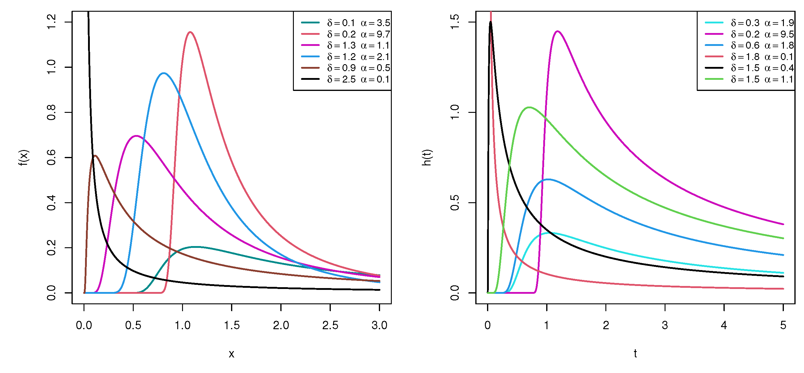
respectively. Putting $\delta =1$ in (1), the Fréchet distribution is acquired as a special case. Various shapes of the density and hazard functions, when $\mu =1$ and some specified values of $\delta$ and $\alpha$, of the LFD-TII are shown in Figure 1. It shows that the density function has a long right tail and that the peak of the distribution decreases when the parameter values of $\delta$ and $\alpha$ increase. Further, the HF plots indicate that the failure rate function has a unimodal shape.

Figure 1. Shapes of density and hazard functions of the LFD-TII.

In the context of reliability experiments, practitioners prefer to deal with a progressive Type-II censoring scheme (PCS-TII) compared to a conventional Type-II (failure) censoring scheme because it allows the removal of survival item(s) during experiments at different stages other than the termination point. Before starting the experiment, n(test sample size), $m(<n)$ (effective sample size) and $R_i,i=1,2,\cdots ,m$ (removal pattern) must be predetermined by the experimenter. When the first failure $x_{1:m:n}$ occurs, the $R_1$ of survival units are randomly drawn from the remaining $n-1$ units. Again, when the second failure $x_{2:m:n}$ occurs, the $R_2$ of survival units are randomly drawn from the remaining $n-1-R_1$ units, and so on. Lastly, when the mth failure $x_{m:m:n}$ occurs, $R_m=n-m-{\sum }_{i=1}^{m-1}{R}_i$ are removed from the test and terminated. For more details, see an excellent monograph published by Balakrishnan and Cramer [3].

In this case, the likelihood function for $x_{i:m:n},i=1,2,\cdots ,m,$ is defined as

$$L\left(\left.\underline{\theta }\right|\mathbf{x}\right)=C{\prod }_{i=1}^{m}f\left(x_{i:m:n};\underline{\theta }\right){\left[1-F\left(x_{i:m:n};\underline{\theta }\right)\right]}^{R_i},$$

(5)

where $C=n(n-1-R_1)\cdots (n-(m-1)-{\sum }_{i=1}^{m-1}{R}_i)$.

In this study, besides the conventional likelihood function (LF) given in (5), the product of spacing (PS) method is also used. This method was independently introduced and discussed by Cheng and Amin [4] and Ranneby [5] as an alternative approach for estimating parameter(s) of continuous univariate distributions.

Following the same philosophy of deriving the maximum likelihood estimators (MLEs), the maximum product of spacing estimators (MPSEs) are derived by determining the parameter choices that maximize the product of the spacings between the ordered values of the target distribution. In addition, in the case of small sample sizes for heavy-tailed or skewed distributions, Anatolyev and Kosenok [6] indicated that the product of spacing estimators are highly efficient compared to the estimators of likelihood method. According to Ng et al. [7], the PS function of PCS-TII data is defined as

$$P\left(\underline{\theta }\right)={\prod }_{i=1}^{m+1}\left[F\left(x_{i:m:n};\underline{\theta }\right)-F\left(x_{i-1:m:n};\underline{\theta }\right)\right]{\prod }_{i=1}^m{\left[1-F\left(x_{i:m:n};\underline{\theta }\right)\right]}^{R_i},$$

(6)

where $F(x_{0:m:n};\underline{\theta })\equiv 0$ and $F(x_{m+1:m:n};\underline{\theta })\equiv 1$.

In the literature, we have not come across any study related to the problem of estimating any unknown parameter of the LFD-TII under any incomplete (censored) data, to the best of our knowledge. To address this gap, the objectives of the present study are fourfold. First, we will mainly focus on both classical and Bayesian estimations to develop the point and interval estimates of $\delta$, $\alpha$, $\mu$, $R\left(t\right)$ and $h\left(t\right)$. Using Fisher’s information, approximate confidence intervals (ACIs) for $\delta$, $\alpha$, $\mu$ or any of their related functions are constructed. Since classical estimators cannot be obtained explicitly, they are evaluated numerically by applying the Newton–Raphson (N-R) method via the ‘maxLik’ package in $\mathsf{R}$ programming software; see Henningsen and Toomet [8]. Using both LF and PS methods, the Bayes estimators against the squared-error loss (SEL) and general-entropy loss (GEL) functions cannot be obtained in closed expressions. To adapt to this problem, utilizing gamma priors, Monte-Carlo Markov-chain (MCMC) techniques are considered to approximate the Bayes estimates and also to construct the highest posterior density (HPD) intervals. Thus, to carry out the Bayesian computations, the ’coda’ package via $\mathsf{R}$ programming software proposed by Plummer et al. [9], which simulates MCMC variates, is used. The second objective discusses how to determine the optimum PCS-TII plan from a set of all possible removal patterns. Third, to compare the performance of the proposed methods, Monte-Carlo simulations are presented. The behavior of the point estimates is compared in terms of their root mean squared-errors (RMSEs) and mean relative absolute biases (MRABs), while the behavior of the interval estimates is compared using their average confidence lengths (ACLs) and coverage probabilities (CPs). The last goal is to demonstrate the suitability and flexibility of the LFD-TII compared to six other popular distributions in modeling real data sets, as well as validating the proposed methodologies in a real-life scenario. We also provide some recommendations.

The next sections of the paper are arranged as follows: Section 2 concerns the classical inference. Bayesian inference is investigated in Section 3. Two-sided ACI/HPD intervals are presented in Section 4. Simulation outputs are presented in Section 5. In Section 6, some criteria of optimal censoring are presented. Two real applications are provided in Section 7. We conclude the article in Section 8.

2. Frequentist Estimation

This section considers the LF and PS methods to derive the point estimators of $\delta$, $\alpha$, $\mu$, $R\left(t\right)$ and $h\left(t\right)$.

2.1. Likelihood Estimators

Suppose $(x_{1:m:n},x_{2:m:n},\cdots ,x_{m:m:n})$ with $(R_1,R_2,\cdots ,R_m)$ is a PCS-TII sample obtained from the LFD-TII. To simplify, $x_i$ is set in place of $x_{i:m:n}$. Substituting (1) and (2) into (5), we can write (5) as

$$\begin{array}{cc}\hfill L\left(\left.\underline{\theta }\right|\mathbf{x}\right)& =C{\left(\delta \alpha {\mu }^{\alpha }\right)}^m{e}^{-{\sum }_{i=1}^m{\rm Y}\left(x_i;\alpha ,\mu \right)}\underset{i=1}{\stackrel{m}{\Pi }}{x}_i^{-\left(\alpha +1\right)}{\left(1-e^{-{\rm Y}(x_i;\alpha ,\mu )}\right)}^{\delta \left(R_i+1\right)-1},\hfill \end{array}$$

(7)

where ${\rm Y}(x_i;\alpha ,\mu )={(\mu /x_i)}^{\alpha },i=1,2,\cdots ,m.$ Taking the natural logarithm of (7) as $\ell (·)\propto logL(·)$ we obtain

$$\begin{array}{cc}\hfill \ell \left(\left.\underline{\theta }\right|\mathbf{x}\right)& \propto mlog\left(\delta \alpha {\mu }^{\alpha }\right)-\alpha \sum _{i=1}^{m}log\left(x_i\right)-\sum _{i=1}^m{\rm Y}\left(x_i;\alpha ,\mu \right)\hfill \\ \hfill & +\sum _{i=1}^m\left(\delta \left(R_i+1\right)-1\right)log\left(1-e^{-{\rm Y}(x_i;\alpha ,\mu )}\right).\hfill \end{array}$$

(8)

Differentiating (8) partially with respect to $\delta$, $\alpha$ and $\mu$, the MLEs $\widehat{\delta }$, $\widehat{\alpha }$ and $\widehat{\mu }$ of $\delta$, $\alpha$ and $\mu$ can be obtained, respectively, by solving the following nonlinear likelihood equations as

$$\frac{\partial \ell }{\partial \delta }=\frac{m}{\delta }+\sum _{i=1}^m\left(R_i+1\right)log\left(1-e^{-{\rm Y}(x_i;\alpha ,\mu )}\right),$$

$$\begin{array}{cc}\hfill \frac{\partial \ell }{\partial \alpha }& =m\left({\alpha }^{-1}+log\left(\mu \right)\right)-\sum _{i=1}^{m}log\left(x_i\right)-\sum _{i=1}^m{{\rm Y}}_{\alpha }^{\prime }\left(x_i;\alpha ,\mu \right)\hfill \\ \hfill & +{\sum _{i=1}^m\left(\delta \left(R_i+1\right)-1\right){{\rm Y}}_{\alpha }^{\prime }\left(x_i;\alpha ,\mu \right)e^{-{\rm Y}(x_i;\alpha ,\mu )}\left(1-e^{-{\rm Y}(x_i;\alpha ,\mu )}\right)}^{-1},\hfill \end{array}$$

and

$$\begin{array}{cc}\hfill \frac{\partial \ell }{\partial \mu }& =\frac{m\alpha }{\mu }-\sum _{i=1}^m{{\rm Y}}_{\mu }^{\prime }\left(x_i;\alpha ,\mu \right)\hfill \\ \hfill & +\sum _{i=1}^m\left(\delta \left(R_i+1\right)-1\right){{\rm Y}}_{\mu }^{\prime }\left(x_i;\alpha ,\mu \right)e^{-{\rm Y}\left(x_i;\alpha ,\mu \right)}{\left(1-e^{-{\rm Y}\left(x_i;\alpha ,\mu \right)}\right)}^{-1},\hfill \end{array}$$

(9)

where ${{\rm Y}}_{\alpha }^{\prime }\left(x_i;\alpha ,\mu \right)={\rm Y}\left(x_i;\alpha ,\mu \right)log\left(\mu /x_i\right)$ and ${{\rm Y}}_{\mu }^{\prime }\left(x_i;\alpha ,\mu \right)={\rm Y}\left(x_i;\alpha ,\mu \right)\left(\alpha /\mu \right),$ for $i=1,2,\cdots ,m.$

From (9), the exact solutions of $\delta$, $\alpha$ and $\mu$ are not available. Thus, for any given data set $(x_i,R_i),i=1,2,\cdots ,m$, the calculated estimates of $\delta$, $\alpha$ or $\mu$ can be easily obtained via the N-R method. Using the invariance characteristic, once the MLEs $\widehat{\delta }$, $\widehat{\alpha }$ and $\widehat{\mu }$ are calculated, the MLEs $\widehat{R}\left(t\right)$ and $\widehat{h}\left(t\right)$ of $R\left(t\right)$ and $h\left(t\right)$, respectively, at time $t>0$ can be easily evaluated.

2.2. Product of Spacings Estimators

The MPSEs of $\delta$, $\alpha$, $\mu$, $R\left(t\right)$ and $h\left(t\right)$ are obtained in this subsection. Thus, following Ng et al. [7], substituting (1) and (2) into (6), the PS function (6) becomes

$$\begin{array}{cc}\hfill P\left(\underline{\theta }\right)& =\prod _{i=1}^{m+1}\left[{\left(1-e^{-{\rm Y}\left(x_{i-1};\alpha ,\mu \right)}\right)}^{\delta }-{\left(1-e^{-{\rm Y}(x_i;\alpha ,\mu )}\right)}^{\delta }\right]\prod _{i=1}^m{{\left(1-e^{-{\rm Y}(x_i;\alpha ,\mu )}\right)}^{\delta }}^{R_i}.\hfill \end{array}$$

(10)

From (10), by maximizing the log-PS function (say, $S(·)\propto logP(·)$), the MPSEs $\widehat{\delta }$, $\widehat{\alpha }$ and $\widehat{\mu }$ of $\delta$, $\alpha$ and $\mu$ can be obtained from the following equation

$$\begin{array}{c}\hfill S\left(\underline{\theta }\right)=\xi \left(\underline{\theta }\right)+\zeta \left(\underline{\theta }\right),\end{array}$$

(11)

where

$$\xi \left(\underline{\theta }\right)={\sum }_{i=1}^{m+1}log\left[{\left(1-e^{-{\rm Y}\left(x_{i-1};\alpha ,\mu \right)}\right)}^{\delta }-{\left(1-e^{-{\rm Y}(x_i;\alpha ,\mu )}\right)}^{\delta }\right],$$

and

$$\zeta \left(\underline{\theta }\right)={\sum }_{i=1}^m\delta R_{i}log\left(1-e^{-{\rm Y}(x_i;\alpha ,\mu )}\right).$$

Differentiating (11) with respect to $\delta$, $\alpha$ and $\mu$, the estimators $\widehat{\delta }$, $\widehat{\alpha }$ and $\widehat{\mu }$ can be obtained as

$$\begin{array}{c}\hfill \widehat{\delta }={\xi }_{\delta }^{\prime }\left(\underline{\theta }\right)+{\zeta }_{\delta }^{\prime }\left(\underline{\theta }\right),\\ \hfill \widehat{\alpha }={\xi }_{\alpha }^{\prime }\left(\underline{\theta }\right)+{\zeta }_{\alpha }^{\prime }\left(\underline{\theta }\right),\end{array}$$

and

$$\begin{array}{c}\hfill \widehat{\mu }={\xi }_{\mu }^{\prime }\left(\underline{\theta }\right)+{\zeta }_{\mu }^{\prime }\left(\underline{\theta }\right),\end{array}$$

(12)

where

$$\begin{array}{cc}\hfill {\xi }_{\delta }^{\prime }\left(\underline{\theta }\right)& ={{\sum }_{i=1}^{m+1}\left[{\overline{F}}_{\delta }^{\prime }\left(x_{i-1}\right)-{\overline{F}}_{\delta }^{\prime }\left(x_i\right)\right]\left[\overline{F}\left(x_{i-1}\right)-\overline{F}\left(x_i\right)\right]}^{-1},\hfill \\ \hfill {\xi }_{\alpha }^{\prime }\left(\underline{\theta }\right)& ={{\sum }_{i=1}^{m+1}\left[{\overline{F}}_{\alpha }^{\prime }\left(x_{i-1}\right)-{\overline{F}}_{\alpha }^{\prime }\left(x_i\right)\right]\left[\overline{F}\left(x_{i-1}\right)-\overline{F}\left(x_i\right)\right]}^{-1},\hfill \\ \hfill {\xi }_{\mu }^{\prime }\left(\underline{\theta }\right)& ={{\sum }_{i=1}^{m+1}\left[{\overline{F}}_{\mu }^{\prime }\left(x_{i-1}\right)-{\overline{F}}_{\mu }^{\prime }\left(x_i\right)\right]\left[\overline{F}\left(x_{i-1}\right)-\overline{F}\left(x_i\right)\right]}^{-1},\hfill \\ \hfill {\zeta }_{\delta }^{\prime }\left(\underline{\theta }\right)& ={\sum }_{i=1}^m{R}_{i}log\left(1-e^{-{\rm Y}(x_i;\alpha ,\mu )}\right),\hfill \\ \hfill {\zeta }_{\alpha }^{\prime }\left(\underline{\theta }\right)& ={\sum }_{i=1}^m\delta R_i{{\rm Y}}_{\alpha }^{\prime }\left(x_i;\alpha ,\mu \right)e^{-{\rm Y}(x_i;\alpha ,\mu )}{\left(1-e^{-{\rm Y}(x_i;\alpha ,\mu )}\right)}^{-1},\hfill \\ \hfill {\zeta }_{\mu }^{\prime }\left(\underline{\theta }\right)& ={\sum }_{i=1}^m\delta R_i{{\rm Y}}_{\mu }^{\prime }\left(x_i;\alpha ,\mu \right)e^{-{\rm Y}(x_i;\alpha ,\mu )}{\left(1-e^{-{\rm Y}(x_i;\alpha ,\mu )}\right)}^{-1},\hfill \\ \hfill F\left(x_w\right)& =1-{\left(1-exp\left(-{\rm Y}\left(x_w;\alpha ,\mu \right)\right)\right)}^{\delta },\forall w=\left(i,i-1\right),\hfill \\ \hfill \overline{F}\left(x_w\right)& ={\left(1-exp\left(-{\rm Y}\left(x_w;\alpha ,\mu \right)\right)\right)}^{\delta },\forall w=\left(i,i-1\right),\hfill \\ \hfill {\overline{F}}_{\delta }^{\prime }\left(x_w\right)& ={\left(1-exp\left(-{\rm Y}\left(x_w;\alpha ,\mu \right)\right)\right)}^{\delta }log\left(1-exp\left(-{\rm Y}\left(x_w;\alpha ,\mu \right)\right)\right),\forall w=\left(i,i-1\right),\hfill \\ \hfill {\overline{F}}_{\alpha }^{\prime }\left(x_w\right)& =\delta {{\rm Y}}_{\alpha }^{\prime }\left(x_w;\alpha ,\mu \right)exp\left(-{\rm Y}\left(x_w;\alpha ,\mu \right)\right){\left(1-exp\left(-{\rm Y}\left(x_w;\alpha ,\mu \right)\right)\right)}^{\delta -1},\forall w=\left(i,i-1\right),\hfill \\ \hfill {\overline{F}}_{\mu }^{\prime }\left(x_w\right)& =\delta {{\rm Y}}_{\mu }^{\prime }\left(x_w;\alpha ,\mu \right)exp\left(-{\rm Y}\left(x_w;\alpha ,\mu \right)\right){\left(1-exp\left(-{\rm Y}\left(x_w;\alpha ,\mu \right)\right)\right)}^{\delta -1},\forall w=\left(i,i-1\right).\hfill \end{array}$$

As it seems from (12), similar to the MLEs, there is no explicit form for the MPSEs. Therefore, the N-R method is utilized to calculate the MPSEs also. Similar to the likelihood estimators, the MPSEs are also consistent, illustrate the invariance principle and provide asymptotic properties. Then, the MPSEs $\widehat{R}\left(t\right)$ and $\widehat{h}\left(t\right)$ of $R\left(t\right)$ and $h\left(t\right)$ can be derived by replacing $\delta$, $\alpha$ and $\mu$ by their $\widehat{\delta }$, $\widehat{\alpha }$ and $\widehat{\mu }$ (for $t>0$), respectively, as

$$\widehat{R}\left(t\right)={(1-e^{-\widehat{{\rm Y}}(t;\widehat{\alpha },\widehat{\mu })})}^{\widehat{\delta }}$$

and

$$\widehat{h}\left(t\right)=\widehat{\delta }\widehat{\alpha }{\widehat{\mu }}^{\widehat{\alpha }}{t}^{-(\widehat{\alpha }+1)}{e}^{-\widehat{{\rm Y}}(t;\widehat{\alpha },\widehat{\mu })}{(1-e^{-\widehat{{\rm Y}}(t;\widehat{\alpha },\widehat{\mu })})}^{-1},$$

where $\widehat{{\rm Y}}(t;\widehat{\alpha },\widehat{\mu })={(\widehat{\mu }/t)}^{\widehat{\alpha }}$.

3. Bayes Procedures

In this section, using both LF and PS approaches, we consider the Bayesian approach to estimate the parameters, reliability and hazard functions of the LFD-TII from PCS-TII data.

3.1. Prior Information and Loss Functions

The selection of prior distributions is an important issue in Bayesian inference. The gamma distribution, depending on its parameter values, gives a variety shapes of its density; see Kundu [10]. Therefore, the gamma density priors are used to adapt support of the LFD-TII parameters. However, the unknown parameters $\delta$, $\alpha$ and $\mu$ are assumed to be stochastically independent, and distributed with gamma conjugate prior distributions such as $\delta \sim Gamma(a_1,b_1)$, $\alpha \sim Gamma(a_2,b_2)$ and $\mu \sim Gamma(a_3,b_3)$.

Thus, the joint PDF of $\delta$, $\alpha$ and $\mu$ is

$$\pi \left(\delta ,\alpha ,\mu \right)\propto {\delta }^{a_1-1}{\alpha }^{a_2-1}{\mu }^{a_3-1}{e}^{-\left(b_1\delta +b_2\alpha +b_3\mu \right)},\delta ,\alpha ,\mu >0,$$

(13)

where $a_i,b_i>0,i=1,2,3$.

The most common loss function in the Bayesian literature is called the SEL function because it assumes that the overestimation and underestimation are treated equally. Under this loss, the Bayes estimate is obtained directly by taking the posterior mean. Therefore, it is clear, concise and fairly easy for inferential issues. Suppose ${\tilde{\nu }}_S$ is an estimate of $\nu$; then, the SEL function is defined as

$$l_S(\nu ,\tilde{\nu })={(\tilde{\nu }-\nu )}^2.$$

(14)

On the other hand, the GEL function is a commonly used asymmetric loss and is defined as

$$l_G(\nu ,\tilde{\nu })={\left(\frac{\tilde{\nu }}{\nu }\right)}^{\tau }-\tau log\left(\frac{\tilde{\nu }}{\nu }\right)-1,\tau \ne 0,$$

(15)

where $\tau$ is a shape parameter. Setting $\tau =-1$ in (15), the Bayes estimate from (15) coincides with the same Bayes estimate from (14). From (15), the minimum of errors occurs when $\tilde{\nu }=\nu$; the positive error has a greater impact than a negative error when $\tau >0$; and the negative error has a greater impact than a positive error when $\tau <0$. Using (15), the Bayes estimate ${\tilde{\nu }}_G$ of $\nu$ is given by

$${\tilde{\nu }}_G={\left[E_{\nu }\left(\left.{\nu }^{-\tau }\right|\mathbf{x}\right)\right]}^{-1/\tau },\tau \ne 0,$$

(16)

where $E_{\nu }(·)$ must exist and be finite.

Next, utilizing both likelihood and spacing functions, we shall develop the Bayes estimates for any parametric function of $\delta$, $\alpha$ and $\mu$ from PCS-TII.

3.2. Posterior Function via Likelihood Data

Following the continuous Bayes’ theorem, based on the likelihood function, the joint posterior PDF (say ${\Psi }_L(·)$) of $\delta$, $\alpha$ and $\mu$ is given by

$${\Psi }_L\left(\left.\delta ,\alpha ,\mu \right|\mathbf{x}\right)=\frac{1}{{\kappa }_1}\pi \left(\delta ,\alpha ,\mu \right)L\left(\left.\delta ,\alpha ,\mu \right|\mathbf{x}\right),$$

(17)

where ${\kappa }_1={\int }_0^{\infty }{\int }_0^{\infty }{\int }_0^{\infty }\pi \left(\delta ,\alpha ,\mu \right)L\left(\left.\delta ,\alpha ,\mu \right|\mathbf{x}\right)\mathrm{d}\delta \mathrm{d}\alpha \mathrm{d}\mu$ is the normalizing constant.

Combining (7) with (13) and substituting into (17), the joint posterior PDF of $\delta$, $\alpha$ and $\mu$ can be written as

$$\begin{array}{cc}\hfill {\Psi }_L\left(\left.\delta ,\alpha ,\mu \right|\mathbf{x}\right)& \propto {\delta }^{m+a_1-1}{\alpha }^{m+a_2-1}{\mu }^{m\alpha +a_3-1}{e}^{-\left(b_1\delta +b_2\alpha +b_3\mu \right)}\hfill \\ \hfill & \times e^{-{\sum }_{i=1}^m{\rm Y}\left(x_i;\alpha ,\mu \right)}\prod _{i=1}^m{x}_i^{-\alpha }{\left(1-e^{-{\rm Y}(x_i;\alpha ,\mu )}\right)}^{\delta \left(R_i+1\right)-1}.\hfill \end{array}$$

(18)

Subsequently, the Bayes estimate of $\delta$, $\alpha$ or $\mu$, say $\Omega (\delta ,\alpha ,\mu )$, under SEL and GEL functions, are given by

$$\begin{array}{c}\hfill {\tilde{\Omega }}_S\left(\delta ,\alpha ,\mu \right)=\frac{1}{{\kappa }_1}{\int }_0^{\infty }{\int }_0^{\infty }{\int }_0^{\infty }\Omega \left(\delta ,\alpha ,\mu \right){\Psi }_L\left(\left.\delta ,\alpha ,\mu \right|\mathbf{x}\right)\mathrm{d}\delta \mathrm{d}\alpha \mathrm{d}\mu ,\end{array}$$

(19)

and

$$\begin{array}{c}\hfill {\tilde{\Omega }}_G\left(\delta ,\alpha ,\mu \right)={\left[\frac{1}{{\kappa }_1}{\int }_0^{\infty }{\int }_0^{\infty }{\int }_0^{\infty }{(\Omega \left(\delta ,\alpha ,\mu \right))}^{-\tau }{\Psi }_L\left(\left.\delta ,\alpha ,\mu \right|\mathbf{x}\right)\mathrm{d}\delta \mathrm{d}\alpha \mathrm{d}\mu \right]}^{-1/\tau },\tau \ne 0,\end{array}$$

(20)

respectively.

From (19) and (20), due to the complex form of (7), the Bayes estimate for any function of $\delta$, $\alpha$ and $\mu$ is obtained in a complex form. For this reason, to obtain the Bayes estimates and also to construct the respective HPD intervals, some MCMC techniques are considered, see Gelman et al. [11]. First, from (18), the conditional distributions of $\delta$, $\alpha$ and $\mu$ are obtained, respectively, as

$${\Psi }_L^{\delta }\left(\left.\delta \right|\alpha ,\mu ,\mathbf{x}\right)\propto {\delta }^{m+a_1-1}{e}^{-\delta b_1^{*}\left(x_i;\alpha ,\mu \right)},$$

(21)

$$\begin{array}{cc}\hfill {\Psi }_L^{\alpha }\left(\left.\alpha \right|\delta ,\mu ,\mathbf{x}\right)& \propto {\alpha }^{m+a_2-1}{\mu }^{m\alpha +a_3-1}{e}^{-b_2\alpha }{e}^{-{\sum }_{i=1}^m{\rm Y}\left(x_i;\alpha ,\mu \right)}\hfill \\ \hfill & \times \prod _{i=1}^m{x}_i^{-\alpha }{\left(1-e^{-{\rm Y}(x_i;\alpha ,\mu )}\right)}^{\delta \left(R_i+1\right)-1},\hfill \end{array}$$

(22)

and

$$\begin{array}{c}\hfill {\Psi }_L^{\mu }\left(\left.\mu \right|\delta ,\alpha ,\mathbf{x}\right)\propto {\mu }^{m\alpha +a_3-1}{e}^{-b_3\mu }{e}^{-{\sum }_{i=1}^m{\rm Y}\left(x_i;\alpha ,\mu \right)}\prod _{i=1}^m{\left(1-e^{-{\rm Y}(x_i;\alpha ,\mu )}\right)}^{\delta \left(R_i+1\right)-1},\end{array}$$

(23)

where $b_1^{*}\left(x_i;\alpha ,\mu \right)=b_1-{\displaystyle \sum _{i=1}^m}\left(R_i+1\right)log\left(1-e^{-{\rm Y}(x_i;\alpha ,\mu )}\right).$

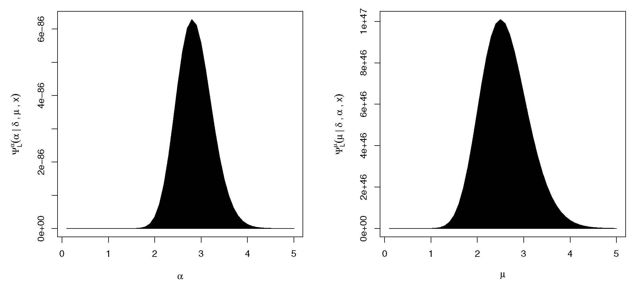
From (21), the conditional PDF of $\delta$ follows $Gamma(m+a_1,b_1^{*}(x_i;\alpha ,\mu ))$. Thus, the samples of $\delta$ can be easily obtained by any gamma generator. From (22) and (23), the conditional posterior distributions of $\alpha$ and $\mu$, respectively, cannot be reduced to any well-known distributions. The diagram plot of the posterior distributions ${\Psi }_L^{\alpha }$ and ${\Psi }_L^{\mu }$, depicted in Figure 2, shows that these distributions behave almost symmetrically. Therefore, Metropolis–Hastings (M-H) is used to simulate MCMC samples from ${\Psi }_L^{\alpha }(·)$ and ${\Psi }_L^{\mu }(·)$.

Figure 2. Diagram plot of the conditional PDFs based on LF of $\alpha$ and $\mu$.

3.3. Posterior Function via Product of Spacing Data

Using a similar fashion of obtaining the Bayes estimates from likelihood data, the joint posterior density of $\delta$, $\alpha$ and $\mu$ based on a PS function, say ${\Psi }_P(·)$, is given by

$${\Psi }_P\left(\left.\delta ,\alpha ,\mu \right|\mathbf{x}\right)=\frac{1}{{\kappa }_2}\pi \left(\delta ,\alpha ,\mu \right)P\left(\left.\delta ,\alpha ,\mu \right|\mathbf{x}\right),$$

(24)

where ${\kappa }_2={\int }_0^{\infty }{\int }_0^{\infty }{\int }_0^{\infty }\pi \left(\delta ,\alpha ,\mu \right)P\left(\left.\delta ,\alpha ,\mu \right|\mathbf{x}\right)\mathrm{d}\delta \mathrm{d}\alpha \mathrm{d}\mu$ is the normalizing constant.

Combining (10) and (13), the joint posterior PDF using the PS function (24) of $\delta$, $\alpha$ and $\mu$ can be expressed as

$$\begin{array}{cc}\hfill {\Psi }_P\left(\left.\delta ,\alpha ,\mu \right|\mathbf{x}\right)& \propto {\delta }^{a_1-1}{\alpha }^{a_2-1}{\mu }^{a_3-1}exp\left(-\left(b_2\alpha +b_3\mu -\sum _{i=1}^{m+1}logG\left(x_i;\delta ,\alpha ,\mu \right)\right)\right)\hfill \\ \hfill & \times exp\left(-\delta \left[b_1-\sum _{i=1}^m{R}_{i}log\left(1-e^{-{\rm Y}(x_i;\alpha ,\mu )}\right)\right]\right),\hfill \end{array}$$

(25)

where $G(x_i;\delta ,\alpha ,\mu )=\left[{\left(1-e^{-{\rm Y}(x_{i-1};\alpha ,\mu )}\right)}^{\delta }-{\left(1-e^{-{\rm Y}(x_i;\alpha ,\mu )}\right)}^{\delta }\right],i=1,2,\cdots ,m+1$.

From (25), the conditional distributions of $\delta$, $\alpha$ and $\mu$ are given, respectively, by

$${\Psi }_P^{\delta }\left(\left.\delta \right|\alpha ,\mu ,\mathbf{x}\right)\propto {\delta }^{a_1-1}exp\left(-\delta \left(b_1-\sum _{i=1}^m{R}_{i}log\left(1-e^{-{\rm Y}\left(x_i;\alpha ,\mu \right)}\right)\right)+\sum _{i=1}^{m+1}logG\left(x_i;\delta ,\alpha ,\mu \right)\right),$$

(26)

$${\Psi }_P^{\alpha }\left(\left.\alpha \right|\delta ,\mu ,\mathbf{x}\right)\propto {\alpha }^{a_2-1}exp\left(-b_2\alpha +\delta \sum _{i=1}^m{R}_{i}log\left(1-e^{-{\rm Y}\left(x_i;\alpha ,\mu \right)}\right)+\sum _{i=1}^{m+1}logG\left(x_i;\delta ,\alpha ,\mu \right)\right),$$

(27)

and

$${\Psi }_P^{\mu }\left(\left.\mu \right|\delta ,\alpha ,\mathbf{x}\right)\propto {\mu }^{a_3-1}exp\left(-b_3\mu +\delta \sum _{i=1}^m{R}_{i}log\left(1-e^{-{\rm Y}\left(x_i;\alpha ,\mu \right)}\right)+\sum _{i=1}^{m+1}logG\left(x_i;\delta ,\alpha ,\mu \right)\right).$$

(28)

As expected, the conditional distributions of $\delta$, $\alpha$ and $\mu$ given by (26), (27) and (28), respectively, cannot follow any standard statistical distribution. Thus, to approximate the Bayesian (point/interval) estimates, the M-H algorithm is proposed to generate MCMC samples from the conditional distributions of $\delta$, $\alpha$ and $\mu$. Now, to generate posterior samples from (18) and (25), the hybrid MCMC algorithm is proposed to obtain the Bayes (point/interval) estimates of $\delta$, $\alpha$, $\mu$, $R\left(t\right)$ or $h\left(t\right)$.

3.4. Hybrid MCMC Algorithm

The hybrid MCMC algorithm, combining the Gibbs sampling (for updating $\delta$) and M-H algorithm sampler (for updating $\alpha$ and $\mu$), is proposed in this subsection. However, to produce MCMC samples via the likelihood function (MCMC-LF) of $\delta$, $\alpha$, $\mu$, $R\left(t\right)$ or $h\left(t\right)$, the following generation process is performed:

Step 1:

Set the initial guesses $({\delta }^{\left(0\right)},{\alpha }^{\left(0\right)},{\mu }^{\left(0\right)})=(\widehat{\delta },\widehat{\alpha },\widehat{\mu })$.

Step 2:

Set $d=1$.

Step 3:

Obtain ${\delta }^{\left(d\right)}$ from $Gamma\left(m+a_1,b_1^{*}\left(x_i;\alpha ,\mu \right)\right)$.

Step 4:

Obtain ${\alpha }^{*}$ and ${\mu }^{*}$ from $N(\widehat{\alpha },{\widehat{\sigma }}_{\alpha }^2)$ and $N(\widehat{\mu },{\widehat{\sigma }}_{\mu }^2)$, respectively, then apply the M-H algorithm as

(a)

Calculate $q_{\alpha }=\frac{{\Psi }_L^{\alpha }\left(\left.{\alpha }^{*}\right|{\delta }^{\left(d\right)},{\mu }^{(d-1)},\mathbf{x}\right)}{{\Psi }_L^{\alpha }\left(\left.{\alpha }^{(d-1)}\right|{\delta }^{\left(d\right)},{\mu }^{(d-1)},\mathbf{x}\right)}$ and $q_{\mu }=\frac{{\Psi }_L^{\mu }\left(\left.{\mu }^{*}\right|{\delta }^{\left(d\right)},{\alpha }^{\left(d\right)},\mathbf{x}\right)}{{\Psi }_L^{\mu }\left(\left.{\mu }^{(d-1)}\right|{\delta }^{\left(d\right)},{\alpha }^{\left(d\right)},\mathbf{x}\right)}$.

(b)

Obtain $Q_{\alpha }=min\{1,q_{\alpha }\}$ and $Q_{\mu }=min\{1,q_{\mu }\}$.

(c)

Obtain $u_1$ and $u_2$ from uniform $U(0,1)$ distribution.

(d)

If $u_1⩽Q_{\alpha }$, set ${\alpha }^{\left(d\right)}={\alpha }^{*}$ else set ${\alpha }^{\left(d\right)}={\alpha }^{(d-1)}$. Repeat this step for $\mu$.

Step 5:

Obtain $R^{\left(d\right)}\left(t\right)$ and $h^{\left(d\right)}(t$) for any time $t>0$ as

$$R^{\left(d\right)}\left(t\right)={\left(1-exp\left(-{\left(\frac{{\mu }^{\left(d\right)}}{t}\right)}^{{\alpha }^{\left(d\right)}}\right)\right)}^{{\delta }^{\left(d\right)}},$$

and

$$h^{\left(d\right)}\left(t\right)={\delta }^{\left(d\right)}{\alpha }^{\left(d\right)}{{\mu }^{\left(d\right)}}^{{\alpha }^{\left(d\right)}}{t}^{-({\alpha }^{\left(d\right)}+1)}{e}^{-{\left(\frac{{\mu }^{\left(d\right)}}{t}\right)}^{{\alpha }^{\left(d\right)}}}{\left(1-exp\left(-{\left(\frac{{\mu }^{\left(d\right)}}{t}\right)}^{{\alpha }^{\left(d\right)}}\right)\right)}^{-1},$$

respectively.

Step 6:

Set $d=d+1$.

Step 7:

Redo Steps 3-6 $\mathcal{N}$ times and ignore the first simulated variates, say ${\mathcal{N}}_0$, as burn-in of $\delta$, $\alpha$, $\mu$, $R\left(t\right)$ and $h\left(t\right)$ (say $\vartheta$) as

$${\vartheta }^{\left(d\right)}=\left({\delta }^{\left(d\right)},{\alpha }^{\left(d\right)},{\mu }^{\left(d\right)},R^{\left(d\right)}\left(t\right),h^{\left(d\right)}\left(t\right)\right),d={\mathcal{N}}_0+1,\cdots ,\mathcal{N}.$$

Step 8:

Obtain the MCMC estimates of $\vartheta$ from (14) and (15), respectively, as

$${\tilde{\vartheta }}_S=\frac{1}{\mathcal{N}-{\mathcal{N}}_0}\sum _{d={\mathcal{N}}_0+1}^{\mathcal{N}}{\vartheta }^{\left(d\right)},$$

and

$${\tilde{\vartheta }}_G={\left[\frac{1}{\mathcal{N}-{\mathcal{N}}_0}\sum _{d={\mathcal{N}}_0+1}^{\mathcal{N}}{\left({\vartheta }^{\left(d\right)}\right)}^{-\tau }\right]}^{-1/\tau },\tau \ne 0.$$

In addition, to develop the Bayesian MCMC estimates utilizing the PS function (MCMC-PS) of $\delta$, $\alpha$, $\mu$, $R\left(t\right)$ or $h\left(t\right)$, one can easily redo the same steps of the M-H algorithm as described in Section 3.4.

4. Interval Estimators

In this section, using the asymptotic normality of the MLEs and MPSEs of $\delta$, $\alpha$, $\mu$, $R\left(t\right)$ and $h\left(t\right)$, the corresponding two-sided ACIs are constructed, see Lawless [12]. Furthermore, using the MCMC simulated variates of the same unknown parameters, the associated HPD intervals are also obtained by implementing the method suggested by Chen and Shao [13].

4.1. Asymptotic Confidence Intervals

To obtain the ACIs for any function of $\delta$, $\alpha$ and $\mu$, a $3\times 3$ asymptotic variance–covariance (V-C) matrix is first obtained by inverting the Fisher information matrix ${\mathbf{I}}_{ij}\left(\underline{\theta }\right)$. According to Lawless [12], the asymptotic V-C matrix, ${\mathbf{I}}^{-1}\left(\underline{\widehat{\theta }}\right)$, for the MLEs $\underline{\widehat{\theta }}={(\widehat{\delta },\widehat{\alpha },\widehat{\mu })}^{\mathsf{T}}$, can be approximated as

$${\mathbf{I}}^{-1}\left(\underline{\widehat{\theta }}\right)\cong {\left[\begin{array}{ccc}-{\mathcal{L}}_{11}& & \\ -{\mathcal{L}}_{21}& -{\mathcal{L}}_{22}& \\ -{\mathcal{L}}_{31}& -{\mathcal{L}}_{32}& -{\mathcal{L}}_{33}\end{array}\right]}_{(\underline{\theta }=\underline{\widehat{\theta }})}^{-1}=\left[\begin{array}{ccc}{\widehat{\sigma }}_{\widehat{\delta }}^2& & \\ {\widehat{\sigma }}_{\widehat{\alpha }\widehat{\delta }}& {\widehat{\sigma }}_{\widehat{\alpha }}^2& \\ {\widehat{\sigma }}_{\widehat{\mu }\widehat{\delta }}& {\widehat{\sigma }}_{\widehat{\mu }\widehat{\alpha }}& {\widehat{\sigma }}_{\widehat{\mu }}^2\end{array}\right].$$

(29)

Similarly, the approximate V-C matrix, ${\mathbf{I}}^{-1}\left(\underline{\widehat{\theta }}\right)$, of the MPSEs $\underline{\widehat{\theta }}={(\widehat{\delta },\widehat{\alpha },\widehat{\mu })}^{\mathsf{T}}$ is given by

$${\mathbf{I}}^{-1}\left(\underline{\widehat{\theta }}\right)\cong {\left[\begin{array}{ccc}-{\mathcal{S}}_{11}& & \\ -{\mathcal{S}}_{21}& -{\mathcal{S}}_{22}& \\ -{\mathcal{S}}_{31}& -{\mathcal{S}}_{32}& -{\mathcal{S}}_{33}\end{array}\right]}_{(\underline{\theta }=\underline{\widehat{\theta }})}^{-1}=\left[\begin{array}{ccc}{\widehat{\sigma }}_{\widehat{\delta }}^2& & \\ {\widehat{\sigma }}_{\widehat{\alpha }\widehat{\delta }}& {\widehat{\sigma }}_{\widehat{\alpha }}^2& \\ {\widehat{\sigma }}_{\widehat{\mu }\widehat{\delta }}& {\widehat{\sigma }}_{\widehat{\mu }\widehat{\alpha }}& {\widehat{\sigma }}_{\widehat{\mu }}^2\end{array}\right],$$

(30)

where ${\mathcal{S}}_{\delta \delta }={\xi }_{\delta }^{″}+{{\zeta }^{″}}_{\delta }$, ${\mathcal{S}}_{\alpha \alpha }={\xi }_{\alpha }^{″}+{\zeta }_{\alpha }^{″}$, ${\mathcal{S}}_{\mu \mu }={\xi }_{\mu }^{″}+{\zeta }_{\mu }^{″}$, ${\mathcal{S}}_{\delta \alpha }={\mathcal{S}}_{\alpha \delta }={\xi }_{\delta \alpha }^{″}+{\zeta }_{\delta \alpha }^{″}$, ${\mathcal{S}}_{\delta \mu }={\mathcal{S}}_{\mu \delta }={\xi }_{\delta \mu }^{″}+{\zeta }_{\delta \mu }^{″}$ and ${\mathcal{S}}_{\alpha \mu }={\mathcal{S}}_{\mu \alpha }={\xi }_{\alpha \mu }^{″}+{\zeta }_{\alpha \mu }^{″}$. From (8) and (11), the Fisher elements in (29) and (30) are obtained and reported as supplementary materials.

To construct the $100(1-\gamma )\%$ two-sided ACI for $R\left(t\right)$ and $h\left(t\right)$, the delta method is considered to estimate these variances, see Greene [14]. Therefore, using this method, the estimated variance of $R\left(t\right)$ and $h\left(t\right)$ at their MLEs $\underline{\theta }=\underline{\widehat{\theta }}$ (or their MPSEs $\underline{\theta }=\underline{\widehat{\theta }}$), are given, respectively, by

$${\sigma }_{R\left(t\right)}^2={\mathcal{D}}_{R\left(t\right)}^{\mathsf{T}}{\mathbf{I}}^{-1}\left(\underline{\theta }\right){\mathcal{D}}_{R\left(t\right)}$$

and

$${\sigma }_{h\left(t\right)}^2={\mathcal{D}}_{h\left(t\right)}^{\mathsf{T}}{\mathbf{I}}^{-1}\left(\underline{\theta }\right){\mathcal{D}}_{h\left(t\right)},$$

where ${\mathcal{D}}_{R\left(t\right)}$ and ${\mathcal{D}}_{h\left(t\right)}$ are the gradient of $R\left(t\right)$ and $h\left(t\right)$ with respect to $\delta$, $\alpha$ and $\mu$, which are given by

$${\mathcal{D}}_{R\left(t\right)}^{\mathsf{T}}=\left[\frac{\partial }{\partial \delta }R\left(t\right),\frac{\partial }{\partial \alpha }R\left(t\right),\frac{\partial }{\partial \mu }R\left(t\right)\right],$$

and

$${\mathcal{D}}_{h\left(t\right)}^{\mathsf{T}}=\left[\frac{\partial }{\partial \delta }h\left(t\right),\frac{\partial }{\partial \alpha }h\left(t\right),\frac{\partial }{\partial \mu }h\left(t\right)\right].$$

Since the MLEs $\underline{\widehat{\theta }}$ and the MPSEs $\underline{\widehat{\theta }}$ are approximately distributed as multivariate normal distribution as $\underline{\widehat{\theta }}\sim \mathcal{N}(\underline{\theta },{\mathbf{I}}^{-1}\left(\underline{\widehat{\theta }}\right))$ and $\underline{\widehat{\theta }}\sim \mathcal{N}(\underline{\theta },{\mathbf{I}}^{-1}\left(\underline{\widehat{\theta }}\right))$, respectively, see Lawless [12], the $100(1-\gamma )\%$ ACI for $\vartheta$ is given by

$$\widehat{\vartheta }\mp z_{\gamma /2}\sqrt{{\widehat{\sigma }}_{\widehat{\vartheta }}^2},$$

where $\widehat{\vartheta }$ denotes the MLE (or MPSE) of $\vartheta$, ${\widehat{\sigma }}_{\widehat{\vartheta }}^2$ is the approximated variance of $\vartheta$ and $z_{\gamma /2}$ is the ${(\gamma /2)}^{th}$ standard normal variate.

4.2. HPD Intervals

To construct the HPD interval of $\delta$, $\alpha$, $\mu$, $R\left(t\right)$ or $h\left(t\right)$, the simulated MCMC-LF samples of ${\vartheta }^{\left(d\right)}$ for $d={\mathcal{N}}_0+1,\cdots ,\mathcal{N}$ must be arranged as ${\vartheta }_{({\mathcal{N}}_0+1)},{\vartheta }_{({\mathcal{N}}_0+2)},\cdots ,{\vartheta }_{\left(\mathcal{N}\right)}$, see Chen and Shao [13]. Thus, the $100(1-\gamma )\%$ two-sided HPD interval of $\vartheta$ is given by

$$\left({\vartheta }_{\left(d^{*}\right)},{\vartheta }_{(d^{*}+(1-\gamma )(\mathcal{N}-{\mathcal{N}}_0))}\right),$$

where $d^{*}={\mathcal{N}}_0+1,\cdots ,\mathcal{N}$ is specified such that

$${\vartheta }_{\left(d^{*}+\left[(1-\gamma )(\mathcal{N}-{\mathcal{N}}_0)\right]\right)}-{\vartheta }_{\left(d^{*}\right)}=\underset{1⩽d⩽\gamma \left(\mathcal{N}-{\mathcal{N}}_0\right)}{min}\left({\vartheta }_{\left(d+\left[(1-\gamma )(\mathcal{N}-{\mathcal{N}}_0)\right]\right)}-{\vartheta }_{\left(d\right)}\right).$$

Here, $\left[w\right]$ represents the largest integer less (or equal) than w.

In a similar manner, the associated HPD intervals of the same unknown parameters depending on the PS approach can be easily obtained.

5. Simulation Study

In this section, the behavior of the proposed frequentist and Bayesian estimators is evaluated through an extensive Monte-Carlo simulation study.

Following Balakrishnan and Cramer [3], for various combinations of n, m and R, we replicated 1,000 times from $\mathrm{LFD}-\mathrm{TII}(0.5,2.5,0.5)$. At mission time $t=0.25$, the corresponding actual value of $R\left(t\right)$ and $h\left(t\right)$ is taken as 0.998 and 0.099, respectively. Taking $n=$40 and 80, the failure percentages (FPs), $\frac{m}{n}\times 100\%$, are used as 50 and 90%. In addition, for each set of n and m, various patterns of $R_i,i=1,2,\cdots ,m$ are used, namely:

$$\begin{array}{cccc}\hfill & \mathrm{Scheme}-1:R_1=n-m,\hfill & \hfill & R_i=0fori\ne 1,\hfill \\ \hfill & \mathrm{Scheme}-2:R_{\frac{m}{2}}=n-m,\hfill & \hfill & R_i=0fori\ne \frac{m}{2},\hfill \\ \hfill & \mathrm{Scheme}-3:R_m=n-m,\hfill & \hfill & R_i=0fori\ne m.\hfill \end{array}$$

In Bayesian calculations, two different sets of hyperparameters for $\delta$, $\alpha$ and $\mu$ are used called, Prior 1: $(a_1,a_2,a_3)=(0.5,2.5,0.5)$ and $b_i=1,i=1,2,3$; and Prior 2: $(a_1,a_2,a_3)=(2,10,2)$ and $b_i=4,i=1,2,3$. Using the hybrid strategy proposed in Section 3.4, we simulate $\mathcal{N}=12,000$ samples from the MCMC-LF (or MCMC-PS) approach and discard the first 2000 values ${\mathcal{N}}_0=2000$ as burn-in. Hence, based on 10,000 MCMC-LF samples, the Bayes estimates and 95% HPD intervals are computed using SEL and GEL (with $\tau =(-5,5)$) functions.

Using the following formulae, the average estimates (AE) of $\delta$, $\alpha$, $\mu$, $R\left(t\right)$ and $h\left(t\right)$, say, ($\varphi$), with their RMSEs and MRABs are calculated, respectively, as

$$\begin{array}{c}\hfill \overline{{\widehat{\varphi }}_{\eta }}=\frac{1}{\mathcal{M}}{\sum }_{i=1}^{\mathcal{M}}{\widehat{\varphi }}_{\eta }^{\left(i\right)},\end{array}$$

$$\begin{array}{c}\hfill \mathrm{RMSE}\left({\widehat{\varphi }}_{\eta }\right)=\sqrt{\frac{1}{\mathcal{M}}{\sum }_{i=1}^{\mathcal{M}}{\left({\widehat{\varphi }}_{\eta }^{\left(i\right)}-{\varphi }_{\eta }\right)}^2},\end{array}$$

and

$$\begin{array}{c}\hfill \mathrm{MRAB}\left({\widehat{\varphi }}_{\eta }\right)=\frac{1}{\mathcal{M}}{\sum }_{i=1}^{\mathcal{M}}\frac{1}{{\varphi }_{\eta }}\left|{\widehat{\varphi }}_{\eta }^{\left(i\right)}-{\varphi }_{\eta }\right|,\end{array}$$

where $\eta =1,2,3,4,5;$$\mathcal{M}$ is the number of generated sequences; ${\widehat{\varphi }}_{\eta }^{\left(i\right)}$ is the calculated estimate obtained at $i^{th}$ sample of ${\varphi }_{\eta }$, ${\varphi }_1=\delta$, ${\varphi }_2=\alpha$, ${\varphi }_3=\mu$, ${\varphi }_4=R\left(t\right)$ and ${\varphi }_5=h\left(t\right)$.

In addition, the ACLs and CPs of $100(1-\gamma )\%$ ACI (or HPD) intervals of ${\varphi }_{\eta }$ are given by

$${\mathrm{ACL}}_{(1-\gamma )\%}\left({\varphi }_{\eta }\right)=\frac{1}{\mathcal{M}}{\sum }_{i=1}^{\mathcal{M}}\left({\mathcal{U}}_{{\widehat{\varphi }}_{\eta }^{\left(i\right)}}\left({\varphi }_{\eta }\right)-{\mathcal{L}}_{{\widehat{\varphi }}_{\eta }^{\left(i\right)}}\left({\varphi }_{\eta }\right)\right),$$

and

$${\mathrm{CP}}_{(1-\gamma )\%}\left({\varphi }_{\eta }\right)=\frac{1}{\mathcal{M}}{\sum }_{j=1}^{\mathcal{M}}{\mathbf{1}}_{\left({\mathcal{L}}_{{\widehat{\varphi }}_{\eta }^{\left(i\right)}};{\mathcal{U}}_{{\widehat{\varphi }}_{\eta }^{\left(i\right)}}\right)}\left({\varphi }_{\eta }\right),$$

respectively, where ${\mathcal{L}}_{{\widehat{\varphi }}_{\eta }^{\left(i\right)}}(·)$ and ${\mathcal{U}}_{{\widehat{\varphi }}_{\eta }^{\left(i\right)}}(·)$ denote the lower and upper sides, respectively, and $\mathbf{1}(·)$ is the indicator function.

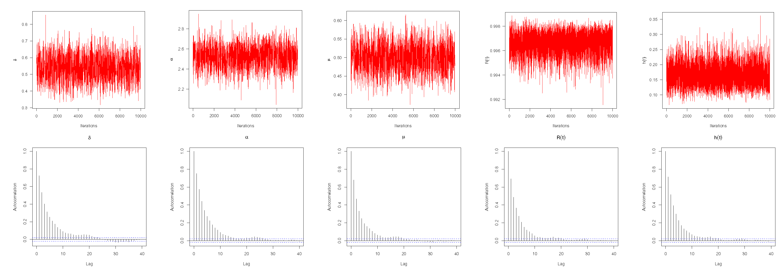
The convergence status of the hybrid MCMC algorithm for the simulated MCMC draws of each unknown parameter is evaluated via both trace and autocorrelation plots (when $(n,m)=(80,40)$ and censoring $(n-m,0^{*}(m-1))$ as an example), see Figure 3. This demonstrates that the trace plots resemble random noise as well as the autocorrelation values close to zero when the lag-value grows. As a result, MCMC draws are appropriately mixed and the estimate results are reasonable.

Figure 3. Trace (top) and autocorrelation (bottom) plots for MCMC draws of $\delta$, $\alpha$, $\mu$, $R\left(t\right)$ and $h\left(t\right)$.

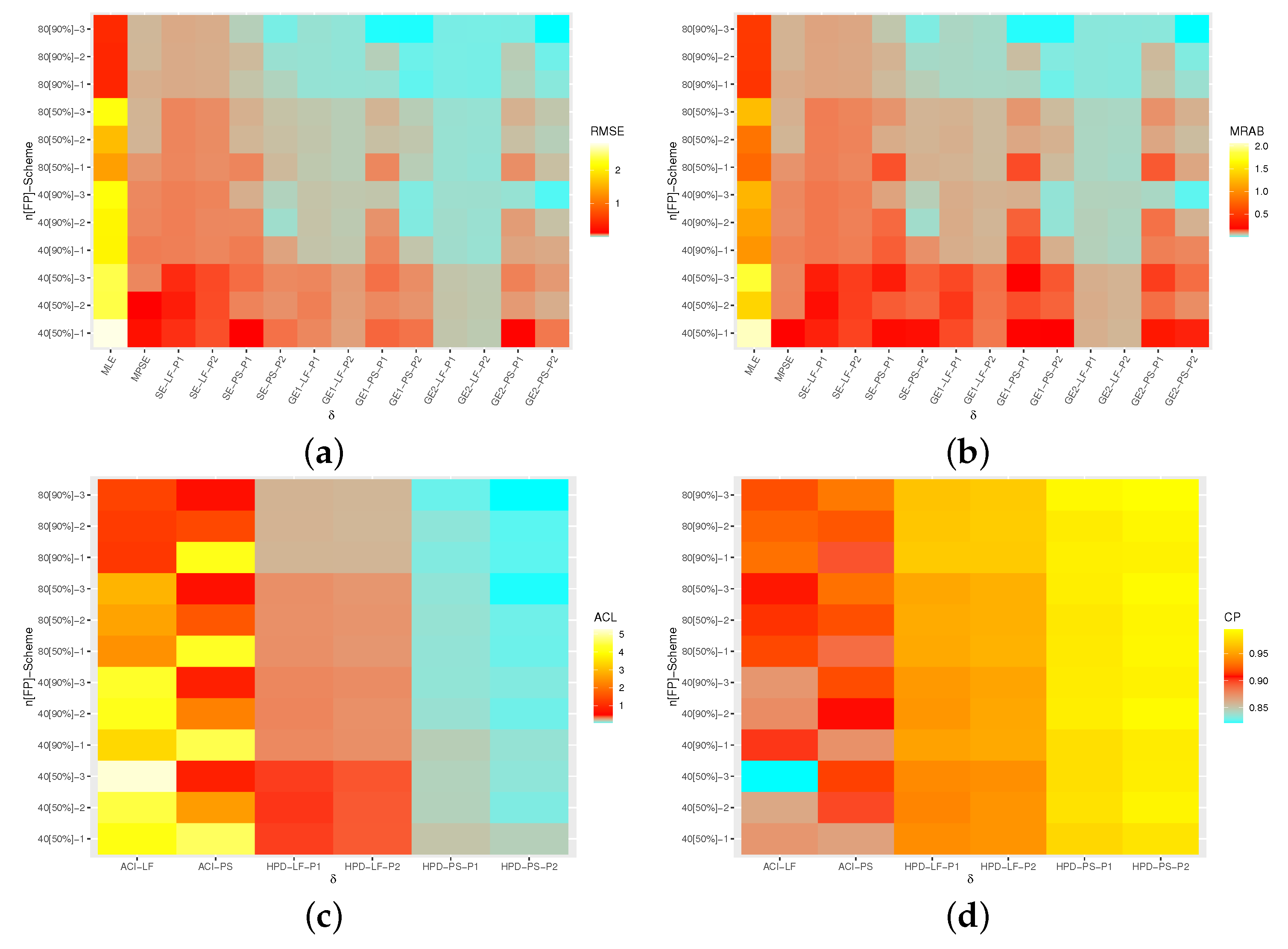
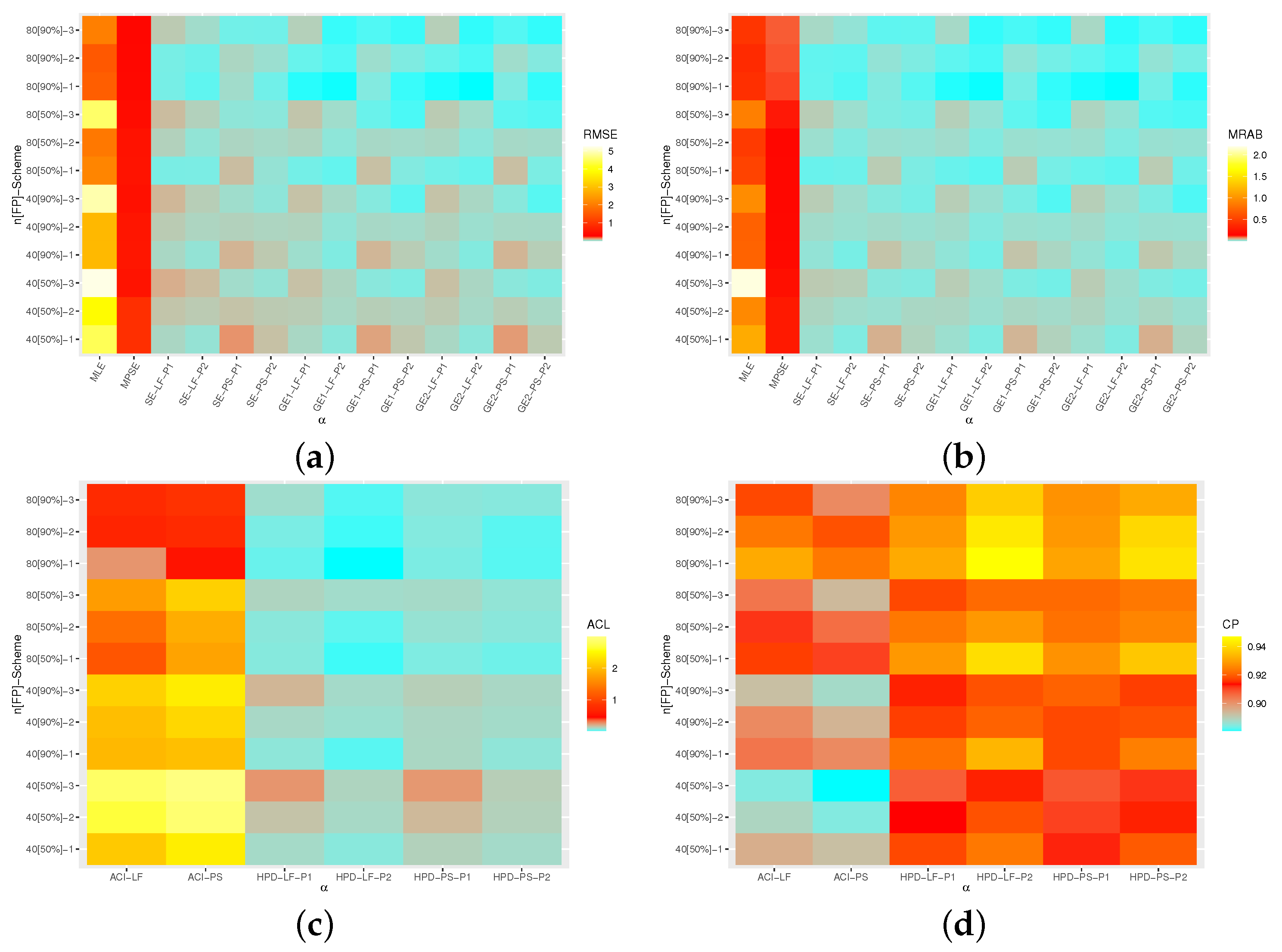
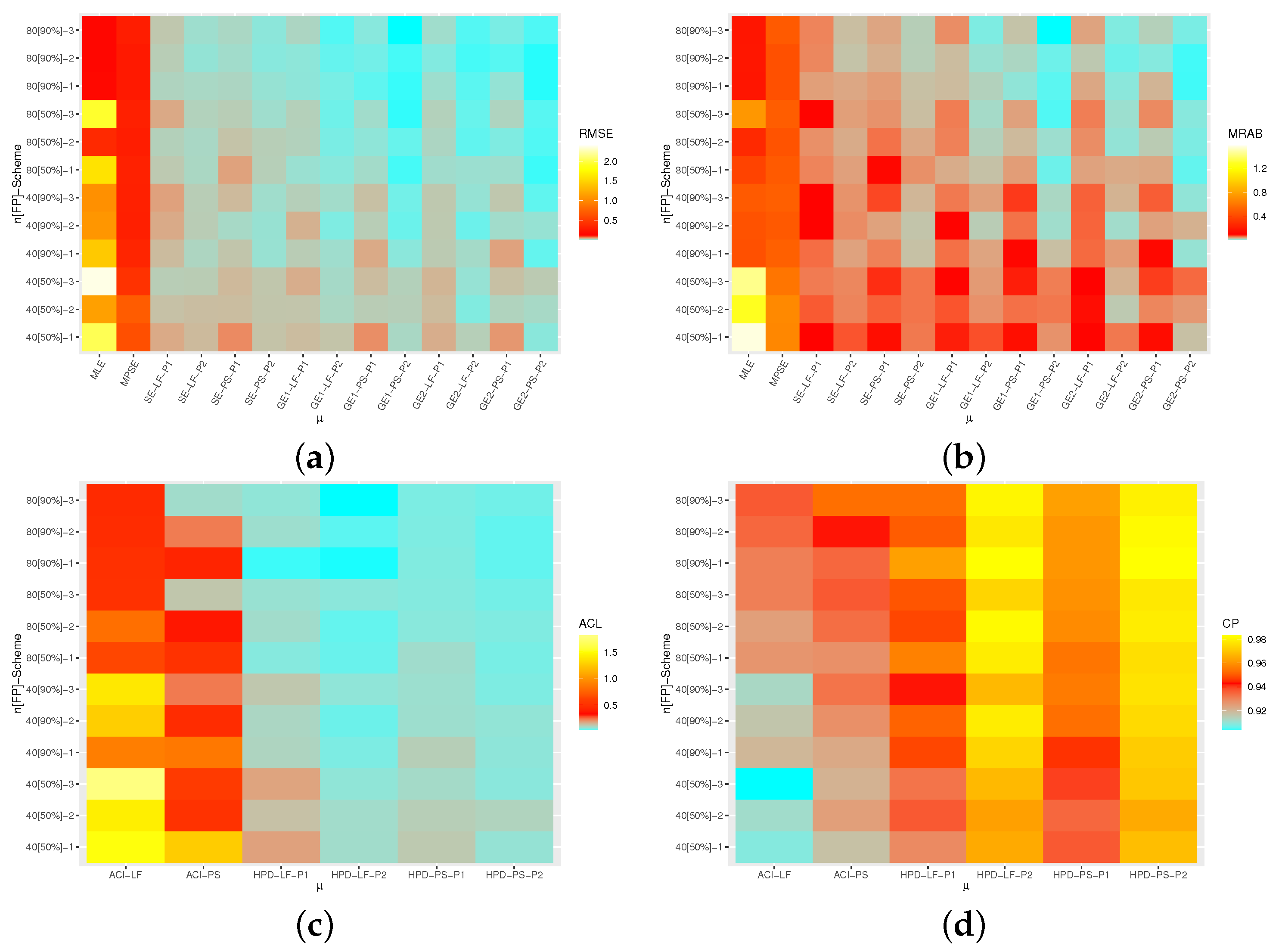
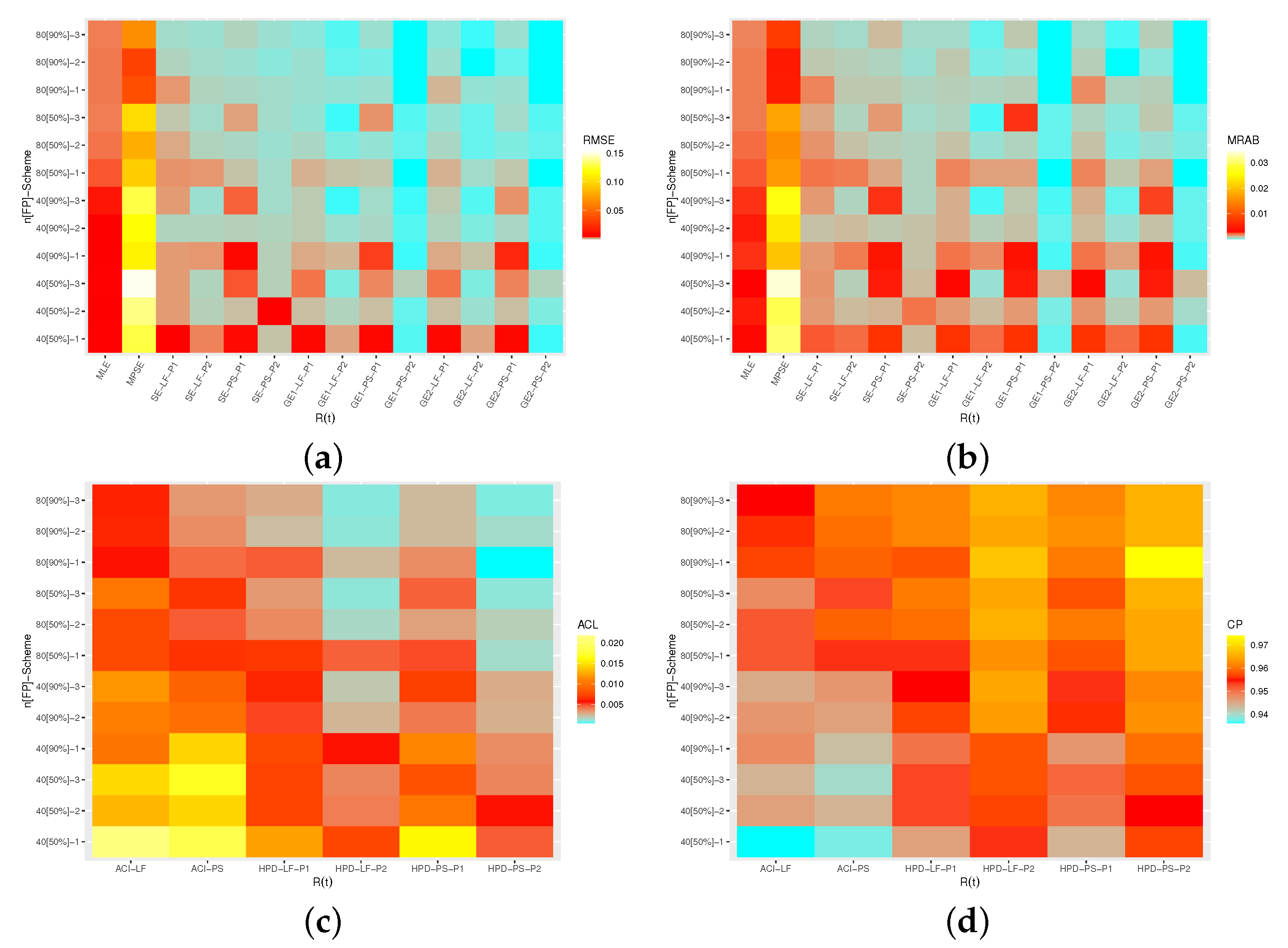
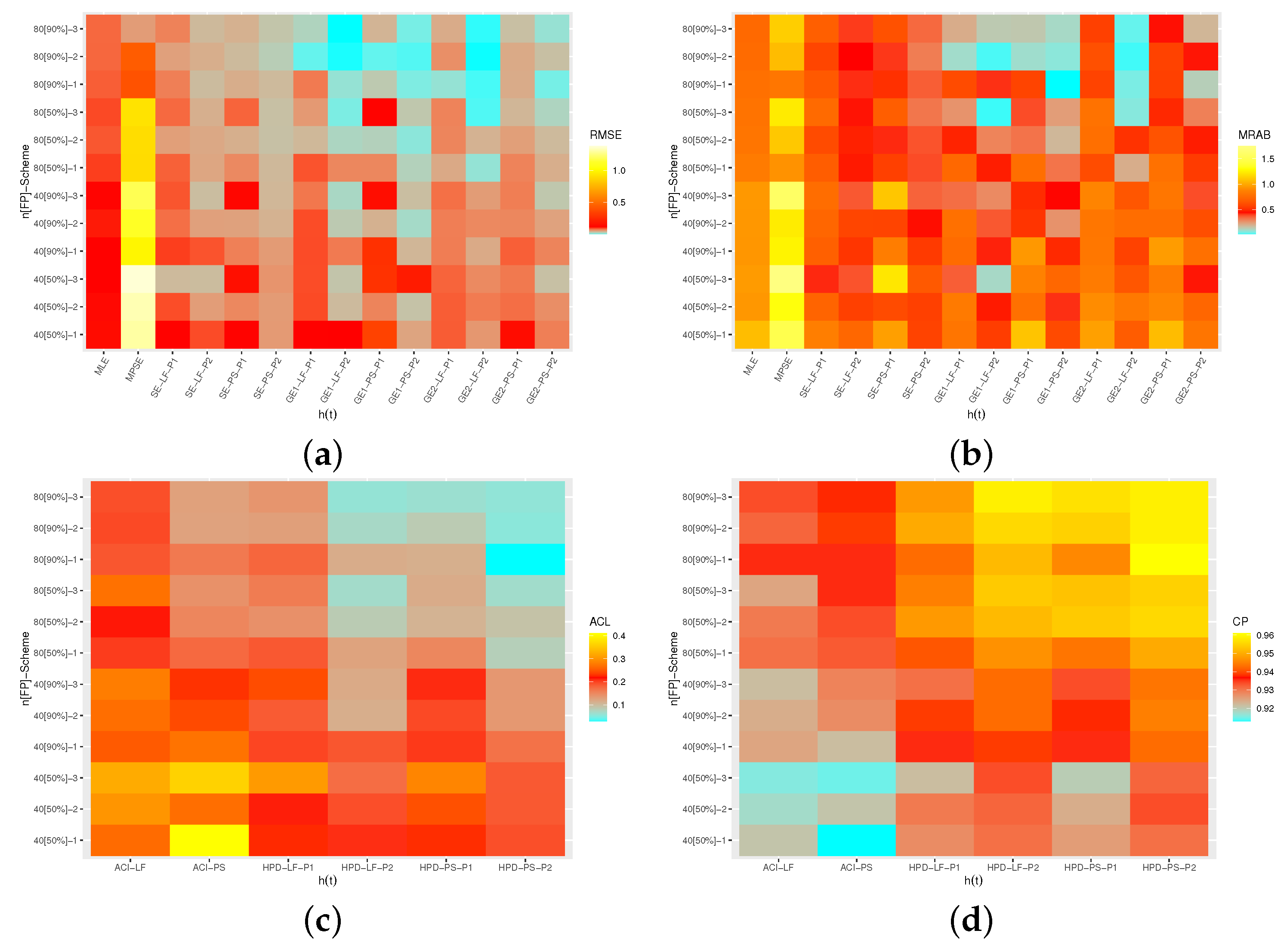
Graphically, the RMSEs, MRABs, ACLs and CPs of $\delta$, $\alpha$, $\mu$, $R\left(t\right)$ and $h\left(t\right)$ are shown with heatmaps, see Figure 4, Figure 5, Figure 6, Figure 7 and Figure 8, respectively, while all simulation results of the same unknown parameters are available in the supplementary file. All numerical evaluations were coded in $\mathsf{R}$ 4.0.4 software. The $\mathsf{R}$ scripts that support the Monte-Carlo findings are available from the corresponding author upon reasonable request. For specification, based on Prior 1 (say, P1) as an example, several notations of the proposed estimation methods are used, such as: Bayes estimates under SEL function from LF method mentioned as “SE-LF-P1”; Bayes estimates under GEL function from LF method for $\tau =(-5,5)$ mentioned as “GE1-LF-P1” and “GE1-LF-P2”, respectively; and the HPD intervals from the LF method denoted as “HPD-LF-P1”.

Figure 4. Heatmap for the simulation results of $\delta$. (a) RMSE. (b) MRAB. (c) ACL. (d) CP.

Figure 5. Heatmap for the simulation results of $\alpha$. (a) RMSE. (b) MRAB. (c) ACL. (d) CP.

Figure 6. Heatmap for the simulation results of $\mu$. (a) RMSE. (b) MRAB. (c) ACL. (d) CP.

Figure 7. Heatmap for the simulation results of $R\left(t\right)$. (a) RMSE. (b) MRAB. (c) ACL. (d) CP.

Figure 8. Heatmap for the simulation results of $h\left(t\right)$. (a) RMSE. (b) MRAB. (c) ACL. (d) CP.

From Figure 4, Figure 5, Figure 6, Figure 7 and Figure 8, we are able to make the following comments:

• All estimates of $\delta$, $\alpha$, $\mu$, $R\left(t\right)$ or $h\left(t\right)$ perform better in terms of lowest RMSEs, MRABs and ACLs as well highest CPs.
• As n (or FP) increases, the proposed estimates become even better than expected. A similar pattern is also observed when ${\sum }_{i=1}^m{R}_i$ decreases.
• Bayesian (point/interval) estimates of all unknown parameters have satisfactory behavior compared to the frequentist (point/interval) estimates, as expected. Since the variance in Prior 2 is lower than the variance in Prior 1, it is observed that the Bayes MCMC estimates using Prior 2 have performed better.
• Bayes estimates of $\delta$, $\alpha$, $\mu$, $R\left(t\right)$ and $h\left(t\right)$ are underestimates (overestimates) when $\tau$ has a positive (negative) value. Meanwhile, the Bayes estimates obtained based on the GEL behave satisfactorily compared to those calculated from the SEL.
• The MPSE/MCMC-PS estimates of $\delta$, $\alpha$ and $\mu$ performed better than others while the MLE/MCMC-LF estimates of $R\left(t\right)$ and $h\left(t\right)$ performed better than others.
• The ACI/HPD interval estimates, in most cases, of $\delta$ and $\mu$ obtained from LF performed better than others while the ACI/HPD interval estimates of $\alpha$, $R\left(t\right)$ and $h\left(t\right)$ obtained from PS performed better than others in terms of the smallest ACLs and largest CPs.
• Comparing the Scheme-1 (first stage) and Scheme-3 (last stage), in terms of their lowest RMSE, MRAB and ACL values as well as their highest CP values, it is clear that the MLE/MCMC-LF estimates for $\delta$, $\alpha$ and $\mu$ are greater under Scheme-3 than -1, while $R\left(t\right)$ and $h\left(t\right)$ are greater under Scheme-1 than Scheme-3.
• The ACLs of the proposed interval estimates obtained by the MPSE/MCMC-PS of all estimates are greater based on Scheme-1 than Scheme-3. In addition, the ACLs of the proposed interval estimates obtained by the MLE/MCMC-LF of $\delta$ and $\alpha$ are narrower under Scheme-1 than Scheme-3, while those associated with $\mu$, $R\left(t\right)$ and $h\left(t\right)$ are greater under Scheme-1 than Scheme-3. The opposite behavior of 95% ACI/HPD intervals is also observed in terms of their CPs.
• To sum up, the Bayes Markov-chain Monte-Carlo approach is recommended to estimate the Type-II Lehmann–Fréchet parameters under progressive censoring.

6. Optimum Censoring

In reliability experiments, one of the most significant challenges for any practitioner is how to select an optimal censoring from a group of all probable plans which provides a significant amount of information about the unknown distribution parameter(s) of interest. To specify the optimum PCS plan $(R_1,R_2,\cdots ,R_m)$, the values of n and m must be fixed in advance; see Ng et al. [15]. In the literature, several authors have also discussed the issue of comparing two (or more) different schemes, see, for example, Pradhan and Kundu [16], Lee and Cho [17], and Elshahhat and Abu El Azm [18], among others.

In this study, using the MLEs/MPSEs of $\underline{\theta }$, several criteria of optimum PCS-TII plans are used, namely:

• $C_1\to \mathrm{Max}\mathrm{trace}\left({\mathbf{I}}_{3\times 3}\left(\underline{\theta }\right)\right)$.
• $C_2\to \mathrm{Min}det\left({\mathbf{I}}_{3\times 3}^{-1}\left(\underline{\theta }\right)\right)$.
• $C_3\to \mathrm{Min}\mathrm{trace}\left({\mathbf{I}}_{3\times 3}^{-1}\left(\underline{\theta }\right)\right)$.
• $C_4\to \mathrm{Min}\widehat{var}(log\left({\mathcal{T}}_{\upsilon }\right))$.
• $C_5\to \mathrm{Min}{\int }_0^1\widehat{var}(log\left({\mathcal{T}}_{\upsilon }\right))w\left(\upsilon \right)d\upsilon$.

Regarding criterion $C_1$, with respect to the MLEs (or MPSEs) of $\delta$, $\alpha$ and $\mu$, the experimenter aims to maximize the trace of Fisher’s elements ${\mathcal{L}}_{11}$, ${\mathcal{L}}_{22}$ and ${\mathcal{L}}_{33}$; regarding criteria $C_2$ and $C_3$, the experimenter aims to minimize the determinant (det) and trace values of the V-C matrices (29) and (30); regarding criterion $C_4$, the experimenter aims to minimize the variance in the logarithmic $\upsilon -th$ quantile, say $log\left({\mathcal{T}}_{\upsilon }\right)$, where $0<\upsilon <1$. From (2), the logarithmic of the quantile function is

$$log\left({\mathcal{T}}_{\upsilon }\right)=log\left[\mu {(-log(1-{(1-\upsilon )}^{1/\delta }))}^{-1/\alpha }\right],0<\upsilon <1.$$

(31)

Using (31), the approximated variance estimate of $log\left({\mathcal{T}}_{\upsilon }\right)$ is given by

$$\widehat{var}\left(log\left({\mathcal{T}}_{\upsilon }\right)\right)={\left[{\mathcal{D}}_{log\left({\mathcal{T}}_{\upsilon }\right)}^{\mathsf{T}}{\mathbf{I}}^{-1}\left(\underline{\theta }\right){\mathcal{D}}_{log\left({\mathcal{T}}_{\upsilon }\right)}\right]}_{(\widehat{\delta },\widehat{\alpha },\widehat{\mu })},$$

where

$${\mathcal{D}}_{log\left({\mathcal{T}}_{\upsilon }\right)}^{\mathsf{T}}={\left[\frac{\partial }{\partial \delta }log\left({\mathcal{T}}_{\upsilon }\right)\phantom{\partial log\left({\mathcal{T}}_{\upsilon }\right)},\frac{\partial }{\partial \alpha }log\left({\mathcal{T}}_{\upsilon }\right),\frac{\partial }{\partial \mu }log\left({\mathcal{T}}_{\upsilon }\right)\right]}_{(\widehat{\delta },\widehat{\alpha },\widehat{\mu })}.$$

7. Real-Life Applications

To examine the applicability of the theoretical results of $\delta$, $\alpha$, $\mu$, $R\left(t\right)$ and $h\left(t\right)$ to a real situation, two real data sets from the engineering and physics fields are analyzed. The first data set (say Data-I), reported by Caroni [19], consists of the number of million rotations before the failure of each of 22 ball bearings. The second data set (say, Data-II), presented by Hinkley [20] and discussed by Elshahhat et al. [21], represents thirty consecutive values of March precipitation (in inches) at Minneapolis/St Paul. Both data sets I and II are reported in Table 1.

Table 1. Ordered lifetime data of ball bearing and March precipitation.

Data	Failure Times
I	17.88, 28.92, 33.00, 41.52, 42.12, 45.60, 48.80, 51.84, 51.96, 54.12, 55.56, 67.80, 68.64, 68.64, 68.88, 84.12, 93.12, 98.64, 105.12, 127.92, 128.04, 173.40
II	0.32, 0.47, 0.52, 0.59, 0.77, 0.81, 0.81, 0.90, 0.96, 1.18, 1.20, 1.20, 1.31, 1.35, 1.43, 1.51, 1.62, 1.74, 1.87, 1.89, 1.95, 2.05, 2.10, 2.20, 2.48, 2.81, 3.00, 3.09, 3.37, 4.75

We first fit the LFD-TII to both complete data sets in Table 1 along with six lifetime models as competitors, namely: inverse Weibull distribution (IWD), Kumaraswamy-inverse Rayleigh distribution (KIRD), Kumaraswamy-inverted exponential distribution (KIED), Kumaraswamy exponentiated inverse Rayleigh distribution (KEIRD), Kumaraswamy-inverse Weibull distribution (KIWD) and Kumaraswamy-inverse Gompertz distribution (KIGD). All the densities of the competing models (for $x>0$ and $\delta ,\alpha ,\mu ,\theta >0$) are reported in Table 2. To select the best model, different criteria are used, namely: (i) the Kolmogorov–Smirnov (K-S) statistic with its p value; (ii) negative log-likelihood (NL); (iii) Akaike’s (A), (iv) consistent Akaike’s (CA); (v) Bayesian (B); and (vi) Hannan–Quinn (HQ) information criteria.

Table 2. Several competing models of Type-II Lehmann–Fréchet distribution.

Model	Density	Author(s)
IWD	$\delta \mu x^{-(\delta +1)}exp(-\mu x^{-\delta })$	Keller et al. [22]
KIRD	$2\delta \mu x^{-3}exp(-\mu x^{-2}){(1-exp(-\mu x^{-2}))}^{\delta -1}$	Hussian and Amin [23]
KIED	$\delta \mu \theta x^{-2}exp(-\theta \mu /x){(1-exp(-\theta \mu /x\left)\right)}^{\delta -1}$	Oguntunde et al. [24]
KEIRD	$2\delta \alpha \mu \theta x^{-3}exp\left(-\alpha \mu \theta x^{-2}\right){(1-exp(-\alpha \mu \theta x^{-2}))}^{\delta -1}$	Haq [25]
KIWD	$\delta \alpha \theta {\mu }^{\alpha }{x}^{-(\alpha +1)}exp(-\theta {(\mu /x)}^{\alpha }){(1-exp(-\theta {(\mu /x)}^{\alpha }))}^{\delta -1}$	Shahbaz et al. [1]
KIGD	$\delta \alpha x^{-2}{e}^{\mu /x}exp(-(\alpha /\mu )(e^{\mu /x}-1)){(1-exp(-(\alpha /\mu )\left(e^{\mu /x}-1\right)))}^{\delta -1}$	El-Morshedy et al. [26]

Via the ‘AdequacyModel’ package in $\mathsf{R}$ programming software proposed by Marinho et al. [27], using the two data sets I and II listed in Table 1, the MLEs of model parameters and selection criteria are computed and provided in Table 3. In addition, the K-S statistics with their p values are listed in Table 4. Among all the fitted lifetime models, Table 3 and Table 4 show that the LFD-TII has the lowest values with respect to NL, A, CA, B, HQ information criteria and K-S statistics, as well as the highest p value. Thus, the LFD-TII provides the best fit, for both given data sets, than all the competitive distributions. As an example, the $\mathsf{R}$ script used to fit the LFD-TII parameters, to evaluate the model selection criteria, and to compute the K-S distance with its p value, is reported in Appendix A.

Table 3. Fitting results of the competitive models based on data sets I and II.

Data	Model	$\widehat{\mathit{\delta }}$	$\widehat{\mathit{\alpha }}$	$\widehat{\mathit{\mu }}$	$\widehat{\mathit{\theta }}$	NL	A	CA	B	HQ
I	LFD-TII	5.3207	0.9900	126.45	-	108.02	222.034	223.367	225.307	222.805
	IWD	1.8549	-	47.549	-	110.05	224.100	224.732	226.283	224.615
	KIRD	1.0562	-	2248.9	-	110.17	224.330	224.962	226.512	224.844
	KIED	5.3140	-	13.659	9.3079	108.02	222.042	223.375	225.315	222.813
	KEIRD	1.0561	12.567	9.1495	19.534	110.17	228.330	230.683	232.695	229.358
	KIWD	28.314	0.5878	21.106	7.0946	107.64	223.272	225.625	227.636	224.300
	KIGD	4.2497	106.45	5.6089	-	108.31	222.622	223.955	225.895	223.393
II	LFD-TII	21.016	0.5422	13.717	-	38.307	82.6149	83.5380	86.8185	83.9597
	IWD	1.5496	-	1.0162	-	41.917	87.8340	88.2785	90.6364	88.9170
	KIRD	0.7316	-	0.6867	-	43.201	90.4023	90.8468	93.2047	91.2989
	KIED	3.3203	-	0.4503	4.9354	39.660	85.3192	86.2422	89.5228	86.6640
	KEIRD	0.7288	0.5041	1.3073	1.0356	43.201	94.4029	96.0029	100.007	96.1959
	KIWD	4.7258	0.8390	1.7612	1.6008	39.170	86.3429	87.9429	91.9477	88.1360
	KIGD	5.9365	3.7276	0.4919	-	38.590	83.1793	84.1023	87.3829	84.5240

Table 4. K-S results under data sets I and II.

Model	Data-I		Data-II
	Statistic	p-Value	Statistic	p-Value
LFD-TII	0.0990	0.9822	0.0841	0.9837
IWD	0.1400	0.7814	0.1524	0.4893
KIRD	0.1478	0.7226	0.1985	0.1880
KIED	0.0884	0.9954	0.1217	0.7658
KEIRD	0.1479	0.7218	0.1990	0.1858
KIWD	0.1124	0.9439	0.1125	0.8420
KIGD	0.1095	0.9545	0.0769	0.9943

Furthermore, Figure 9 display (i) the histogram plot of data sets I and II and the estimated densities and (ii) the plot of estimated and empirical reliability parameters. It shows that the LFD-TII is the best lifetime model among other competing models for both data sets I and II. It also supports the same findings listed in Table 3 and Table 4.

Figure 9. Plots of the fitted PDFs (left) and fitted RFs (right) of LFD-TII and its competing models based on data sets I and II.

From Table 1, taking $m=10$, three different PCS-TII samples are obtained and provided in Table 5, where the censoring plan $R=(4,0,0,0,4)$ is referred as $R=(4,0^3,4)$ for short. Since we do not have any prior information on $\delta$, $\alpha$ and $\mu$, the Bayes estimates based on SEL and GEL (for $\tau (=-3,-0.03,+3)$) are developed using the improper gamma prior. We also take 0.0001 for all given hyperparameters. Using the MCMC algorithm described in Section 3, for each unknown parameter, the first 10,000 simulated values of 50,000 MCMC samples are discarded. To run the MCMC sampler, the frequentist estimates of $\delta$, $\alpha$ and $\mu$ are used as initial values. According to the LF and PS methods, using each sample in Table 5, the point estimates with their standard errors (St.Es) as well as the interval estimates with their lengths of $\delta$, $\alpha$, $\mu$, $R\left(t\right)$ and $h\left(t\right)$ are calculated and reported in Table 6 and Table 7. The acquired estimators of $R\left(t\right)$ and $h\left(t\right)$ are evaluated at $t=50$ and 1 for data sets I and II, respectively. It is observed, from Table 6 and Table 7, that the Bayes MCMC estimates of all unknown parameters performed better than the frequentist approaches in terms of the minimum St.Es, as well as, the HPD interval estimates also behaving better than others in terms of the shortest lengths.

Table 5. Three different generated progressively censored data sets.

Data	Scheme	PCS-TII Data
I	${\mathcal{R}}_1=(12,0^9)$	17.88, 28.92, 42.12, 51.96, 55.56, 68.64, 84.12, 98.64, 105.12, 128.04
	${\mathcal{R}}_2=(0^4,6^2,0^4)$	17.88, 28.92, 33.00, 41.52, 42.12, 51.96, 67.80, 68.64, 93.12, 105.12
	${\mathcal{R}}_3=(0^9,12)$	17.88, 28.92, 33.00, 41.52, 42.12, 45.60, 48.80, 51.84, 51.96, 54.12
II	${\mathcal{R}}_1=(20,0^9)$	0.32, 0.77, 0.81, 0.96, 1.18, 1.43, 1.51, 2.05, 2.48, 3.09
	${\mathcal{R}}_2=(0^4,{10}^2,0^4)$	0.32, 0.47, 0.52, 0.59, 0.77, 1.18, 1.74, 1.87, 2.48, 3.00
	${\mathcal{R}}_3=(0^9,20)$	0.32, 0.47, 0.52, 0.59, 0.77, 0.81, 0.81, 0.90, 0.96, 1.18

Table 6. Point estimates (first column) with their St.Es (second column) of $\delta$, $\alpha$, $\mu$, $R\left(t\right)$ and $h\left(t\right)$ based on data sets I and II.

Data		Par.	Classical		SEL		GEL
$\mathit{\tau }\to$							−3		−0.03		3
			LF Approach
I	${\mathcal{R}}_1$	$\delta$	73.056	9.5317	73.030	0.0002	73.030	0.0262	73.030	0.0262	73.030	0.0263
		$\alpha$	0.4665	0.0233	0.4620	0.0001	0.4629	0.0036	0.4615	0.0050	0.4601	0.0065
		$\mu$	1691.0	3.2292	1690.9	0.0005	1690.9	0.0999	1690.9	0.0999	1690.9	0.0999
		$R\left(50\right)$	0.6590	0.1100	0.6289	0.0005	0.6458	0.0132	0.6198	0.0392	0.5874	0.0716
		$h\left(50\right)$	0.0202	0.0056	0.0217	0.0001	0.0231	0.0029	0.0211	0.0009	0.0186	0.0016
	${\mathcal{R}}_2$	$\delta$	160.21	13.642	160.19	0.0002	160.19	0.0261	160.19	0.0262	160.19	0.0262
		$\alpha$	0.4627	0.0151	0.4612	0.0001	0.4617	0.0010	0.4610	0.0017	0.4604	0.0023
		$\mu$	2506.5	9.8757	2506.4	0.0005	2506.4	0.1037	2506.4	0.1037	2506.4	0.1037
		$R\left(50\right)$	0.7023	0.0869	0.6870	0.0004	0.6969	0.0055	0.6819	0.0204	0.6644	0.0379
		$h\left(50\right)$	0.0200	0.0053	0.0210	0.0001	0.0222	0.0022	0.0204	0.0004	0.0182	0.0018
	${\mathcal{R}}_3$	$\delta$	154.08	7.4435	154.05	0.0003	154.05	0.0252	154.05	0.0252	154.05	0.0253
		$\alpha$	0.5284	0.0163	0.5267	0.0001	0.5271	0.0013	0.5264	0.0020	0.5257	0.0027
		$\mu$	1403.9	4.3632	1403.8	0.0005	1403.8	0.1013	1403.8	0.1013	1403.8	0.1013
		$R\left(50\right)$	0.6341	0.0901	0.6195	0.0004	0.6315	0.0025	0.6133	0.0207	0.5923	0.0418
		$h\left(50\right)$	0.0281	0.0064	0.0293	0.0001	0.0306	0.0025	0.0286	0.0005	0.0263	0.0018
II	${\mathcal{R}}_1$	$\delta$	52.308	10.023	52.286	0.0002	52.286	0.0228	52.286	0.0229	52.286	0.0229
		$\alpha$	0.4639	0.0285	0.4599	0.0001	0.4610	0.0030	0.4593	0.0046	0.4576	0.0063
		$\mu$	30.930	2.7366	30.833	0.0005	30.834	0.0961	30.833	0.0966	30.833	0.0971
		$R\left(1\right)$	0.6801	0.1050	0.6527	0.0005	0.6677	0.0124	0.6447	0.0354	0.6163	0.0638
		$h\left(1\right)$	0.8821	0.2443	0.9437	0.0012	0.9983	0.1163	0.9150	0.0329	0.8135	0.0686
	${\mathcal{R}}_2$	$\delta$	419.81	12.008	419.79	0.0003	419.79	0.0289	419.79	0.0289	419.79	0.0289
		$\alpha$	0.2910	0.0069	0.2910	0.0001	0.2911	0.0001	0.2909	0.0001	0.2907	0.0003
		$\mu$	1009.1	1.5645	1009.1	0.0003	1009.1	0.0261	1009.1	0.0261	1009.1	0.0261
		$R\left(1\right)$	0.7901	0.0663	0.7827	0.0003	0.7880	0.0021	0.7800	0.0100	0.7710	0.0191
		$h\left(1\right)$	0.5135	0.1463	0.5299	0.0007	0.5683	0.0548	0.5105	0.0029	0.4459	0.0676
	${\mathcal{R}}_3$	$\delta$	813.14	11.876	813.12	0.0003	813.12	0.0266	813.12	0.0266	813.12	0.0266
		$\alpha$	0.2475	0.0049	0.2475	0.0001	0.2476	0.0002	0.2475	0.0001	0.2474	0.0001
		$\mu$	4249.0	0.7103	4249.0	0.0002	4249.0	0.0277	4249.0	0.0277	4249.0	0.0277
		$R\left(1\right)$	0.7408	0.0715	0.7358	0.0003	0.7420	0.0012	0.7327	0.0081	0.7219	0.0189
		$h\left(1\right)$	0.5870	0.1534	0.5997	0.0007	0.6358	0.0487	0.5818	0.0053	0.5209	0.0662
			PS Approach
I	${\mathcal{R}}_1$	$\delta$	48.600	15.867	48.531	0.0004	48.531	0.0692	48.531	0.0694	48.531	0.0696
		$\alpha$	0.5926	0.0455	0.5824	0.0002	0.5841	0.0084	0.5815	0.0110	0.5789	0.0137
		$\mu$	723.00	6.3394	722.90	0.0005	722.90	0.0994	722.90	0.0994	722.90	0.0994
		$R\left(50\right)$	0.6875	0.1186	0.6447	0.0005	0.6624	0.0251	0.6352	0.0524	0.5993	0.0882
		$h\left(50\right)$	0.0217	0.0069	0.0241	0.0001	0.0256	0.0039	0.0232	0.0015	0.0204	0.0013
	${\mathcal{R}}_2$	$\delta$	48.323	7.3799	48.260	0.0004	48.261	0.0628	48.260	0.0630	48.260	0.0632
		$\alpha$	0.6977	0.0350	0.6880	0.0002	0.6893	0.0084	0.6874	0.0104	0.6854	0.0124
		$\mu$	499.90	1.1073	499.80	0.0005	499.80	0.0989	499.80	0.0990	499.80	0.0990
		$R\left(50\right)$	0.7178	0.0890	0.6845	0.0004	0.6948	0.0230	0.6791	0.0387	0.6601	0.0577
		$h\left(50\right)$	0.0231	0.0060	0.0253	0.0001	0.0265	0.0033	0.0246	0.0015	0.0225	0.0006
	${\mathcal{R}}_3$	$\delta$	12.086	8.7069	12.022	0.0004	12.023	0.0634	12.022	0.0642	12.021	0.0650
		$\alpha$	0.9979	0.1504	0.9621	0.0003	0.9657	0.0322	0.9603	0.0375	0.9547	0.0431
		$\mu$	168.95	1.9830	168.86	0.0005	168.86	0.0980	168.86	0.0981	168.86	0.0981
		$R\left(50\right)$	0.6552	0.0963	0.6122	0.0003	0.6199	0.0353	0.6082	0.0470	0.5949	0.0603
		$h\left(50\right)$	0.0289	0.0137	0.0308	0.0001	0.0311	0.0022	0.0306	0.0017	0.0300	0.0011
II	${\mathcal{R}}_1$	$\delta$	8.5676	9.9608	8.4808	0.0004	8.5016	0.0660	8.5005	0.0672	8.4993	0.0683
		$\alpha$	0.9330	0.4239	0.8809	0.0004	0.8870	0.0460	0.8779	0.0550	0.8686	0.0643
		$\mu$	3.4884	3.2439	3.3926	0.0005	3.3955	0.0929	3.3912	0.0972	3.3868	0.1016
		$R\left(1\right)$	0.7021	0.1246	0.6252	0.0004	0.6347	0.0674	0.6204	0.0818	0.6046	0.0976
		$h\left(1\right)$	1.0805	0.4127	1.2270	0.0007	1.2420	0.1614	1.2191	0.1386	1.1912	0.1107
	${\mathcal{R}}_2$	$\delta$	997.07	16.797	997.06	0.0001	997.06	0.0062	997.06	0.0062	997.06	0.0062
		$\alpha$	0.2891	0.0060	0.2892	0.0001	0.2894	0.0003	0.2892	0.0001	0.2890	0.0001
		$\mu$	1602.8	0.4502	1602.8	0.0002	1602.8	0.0256	1602.8	0.0256	1602.8	0.0256
		$R\left(1\right)$	0.8063	0.0653	0.8003	0.0003	0.8055	0.0008	0.7975	0.0088	0.7883	0.0181
		$h\left(1\right)$	0.5252	0.1632	0.5412	0.0008	0.5909	0.0657	0.5163	0.0090	0.4352	0.0900
	${\mathcal{R}}_3$	$\delta$	63.886	1.2808	63.880	0.0001	63.880	0.0065	63.880	0.0065	63.880	0.0065
		$\alpha$	0.3315	0.0122	0.3306	0.0001	0.3310	0.0005	0.3304	0.0011	0.3298	0.0017
		$\mu$	167.77	0.1759	167.75	0.0002	167.75	0.0249	167.75	0.0249	167.75	0.0249
		$R\left(1\right)$	0.7626	0.0706	0.7513	0.0003	0.7574	0.0052	0.7482	0.0144	0.7376	0.0250
		$h\left(1\right)$	0.4921	0.1197	0.5094	0.0006	0.5352	0.0431	0.4964	0.0043	0.4522	0.0399

Table 7. Interval estimates of $\delta$, $\alpha$, $\mu$, $R\left(t\right)$ and $h\left(t\right)$ based on data sets I and II.

Data	Scheme	Par.	ACI						HPD
			MLE			MPSE			LF			PS
			Lower	Upper	Length	Lower	Upper	Length	Lower	Upper	Length	Lower	Upper	Length
I	${\mathcal{R}}_1$	$\delta$	54.374	91.738	37.364	17.502	79.699	62.197	72.938	73.129	0.1911	48.380	48.688	0.3078
		$\alpha$	0.4209	0.5121	0.0912	0.5033	0.6818	0.1785	0.4192	0.5009	0.0817	0.5202	0.6443	0.1240
		$\mu$	1684.6	1697.3	12.658	710.58	735.43	24.850	1690.7	1691.0	0.3692	722.72	723.09	0.3704
		$R\left(50\right)$	0.4435	0.8745	0.4311	0.4550	0.9201	0.4650	0.4268	0.8299	0.4030	0.4269	0.8418	0.4149
		$h\left(50\right)$	0.0091	0.0312	0.0221	0.0082	0.0352	0.0270	0.0113	0.0324	0.0211	0.0126	0.0365	0.0239
	${\mathcal{R}}_2$	$\delta$	133.47	186.95	53.477	33.859	62.788	28.929	160.08	160.28	0.1911	48.109	48.403	0.2945
		$\alpha$	0.4331	0.4923	0.0592	0.6291	0.7663	0.1372	0.4353	0.4901	0.0548	0.6304	0.7486	0.1183
		$\mu$	2487.2	2525.9	38.712	497.73	502.07	4.3404	2506.2	2506.6	0.3765	499.61	499.99	0.3748
		$R\left(50\right)$	0.5320	0.8727	0.3407	0.5433	0.8923	0.3490	0.5340	0.8545	0.3205	0.5165	0.8452	0.3288
		$h\left(50\right)$	0.0097	0.0303	0.0206	0.0114	0.0349	0.0235	0.0108	0.0305	0.0197	0.0144	0.0362	0.0219
	${\mathcal{R}}_3$	$\delta$	139.49	168.67	29.178	0.0001	29.151	29.151	153.96	154.15	0.1965	11.877	12.181	0.3049
		$\alpha$	0.4965	0.5602	0.0637	0.7031	1.2926	0.5896	0.4981	0.5589	0.0608	0.8504	1.0788	0.2284
		$\mu$	1395.4	1412.5	17.104	165.07	172.84	7.7730	1403.7	1404.0	0.3679	168.64	169.03	0.3896
		$R\left(50\right)$	0.4575	0.8106	0.3532	0.4664	0.8440	0.3776	0.4499	0.7835	0.3336	0.4790	0.7467	0.2678
		$h\left(50\right)$	0.0155	0.0407	0.0252	0.0020	0.0558	0.0538	0.0167	0.0411	0.0244	0.0241	0.0367	0.0126
II	${\mathcal{R}}_1$	$\delta$	32.664	71.953	39.290	0.0001	28.090	28.090	52.191	52.382	0.1912	8.3324	8.6587	0.3263
		$\alpha$	0.4081	0.5198	0.1117	0.1022	1.7638	1.6616	0.4180	0.5070	0.0890	0.7381	1.0230	0.2850
		$\mu$	25.566	36.293	10.727	0.0001	9.8462	9.8462	30.651	31.031	0.3800	3.2065	3.5888	0.3823
		$R\left(1\right)$	0.4743	0.8860	0.4117	0.4580	0.9463	0.4882	0.4518	0.8371	0.3853	0.4560	0.7649	0.3089
		$h\left(1\right)$	0.4033	1.3609	0.9576	0.2717	1.8893	1.6176	0.5139	1.4045	0.8906	0.9580	1.4778	0.5198
	${\mathcal{R}}_2$	$\delta$	396.28	443.35	47.070	964.15	1030.0	65.843	419.68	419.88	0.1975	997.01	997.11	0.0995
		$\alpha$	0.2775	0.3045	0.0270	0.2772	0.3009	0.0237	0.2777	0.3041	0.0264	0.2774	0.3012	0.0238
		$\mu$	1006.0	1012.1	6.1327	1601.9	1603.7	1.7646	1008.9	1009.1	0.1966	1602.7	1602.9	0.1916
		$R\left(1\right)$	0.6602	0.9200	0.2598	0.6784	0.9343	0.2559	0.6604	0.9064	0.2460	0.6730	0.9197	0.2467
		$h\left(1\right)$	0.2267	0.8003	0.5736	0.2053	0.8452	0.6399	0.2523	0.8034	0.5511	0.2384	0.8652	0.6267
	${\mathcal{R}}_3$	$\delta$	789.87	836.42	46.552	61.376	66.397	5.0206	813.02	813.22	0.1994	63.831	63.928	0.0978
		$\alpha$	0.2379	0.2570	0.0191	0.3077	0.3554	0.0478	0.2389	0.2576	0.0188	0.3081	0.3538	0.0457
		$\mu$	4247.6	4250.4	2.7842	167.43	168.12	0.6897	4248.9	4249.1	0.1868	167.65	167.84	0.1943
		$R\left(1\right)$	0.6007	0.8809	0.2801	0.6242	0.9009	0.2767	0.6031	0.8674	0.2643	0.6114	0.8736	0.2622
		$h\left(1\right)$	0.2864	0.8877	0.6012	0.2575	0.7267	0.4693	0.3178	0.8936	0.5757	0.2958	0.7435	0.4478

Using the estimated variances and covariances of MLEs and MPSEs, for data sets I and II, the problem of selecting the optimum PCS-TII censoring is discussed and listed in Table 8. To distinguish, the selected optimal censoring scheme is marked with an asterisk. From Table 8, it is noted that

Table 8. Optimum PCS-TII plan from data sets I and II.

Data	Scheme	${\mathit{C}}_1$	${\mathit{C}}_2$	${\mathit{C}}_3$	${\mathit{C}}_4$
					${\mathbf{C}}_{\mathbf{5}}$
$\mathbf{\upsilon }\to$					0.3	0.6	0.9
LF Approach
I	${\mathcal{R}}_1$	2082.015	101.2823	0.389996	62.52783	112.7259	233.2256
					11.90311	37.69464	85.23925
	${\mathcal{R}}_2$	${}^{*}$ 4688.305	283.6424	1.719240	38.36798	65.59991	122.6290
					7.502976	22.88584	49.32795
	${\mathcal{R}}_3$	3891.927	${}^{*}$ 74.44370	${}^{*}$ 0.174372	${}^{*}$ 22.93697	${}^{*}$ 35.75104	${}^{*}$ 59.00037
					${}^{*}$ 4.757512	${}^{*}$ 13.49737	${}^{*}$ 27.07779
II	${\mathcal{R}}_1$	1785.684	${}^{*}$ 107.9508	0.417767	${}^{*}$ 0.029229	${}^{*}$ 0.055956	${}^{*}$ 0.141237
					${}^{*}$ 0.004819	${}^{*}$ 0.017898	${}^{*}$ 0.043607
	${\mathcal{R}}_2$	21164.55	146.6347	0.016392	0.037272	0.085652	0.217545
					0.006003	0.023741	0.064289
	${\mathcal{R}}_3$	${}^{*}$ 42203.38	141.5372	${}^{*}$ 0.001686	0.038252	0.079309	0.219933
					0.005486	0.020675	0.060050
PS Approach
I	${\mathcal{R}}_1$	810.7222	291.9464	10.95177	62.02883	97.68337	235.7884
					13.66927	37.09831	80.02598
	${\mathcal{R}}_2$	${}^{*}$ 949.3561	${}^{*}$ 55.68957	${}^{*}$ 0.070385	${}^{*}$ 21.93534	${}^{*}$ 42.03723	${}^{*}$ 72.05208
					${}^{*}$ 6.154700	${}^{*}$ 17.30182	${}^{*}$ 33.26023
	${\mathcal{R}}_3$	188.1588	79.76426	1.561285	29.40803	98.88016	844.3476
					6.671761	20.66986	114.7031
II	${\mathcal{R}}_1$	75.72609	109.9195	1.507518	${}^{*}$ 0.027046	${}^{*}$ 0.055033	${}^{*}$ 0.166123
					${}^{*}$ 0.005775	${}^{*}$ 0.018031	${}^{*}$ 0.053759
	${\mathcal{R}}_2$	${}^{*}$ 27426.55	282.3439	0.002085	0.034347	0.072679	0.280724
					0.006669	0.021365	0.053968
	${\mathcal{R}}_3$	6812.186	${}^{*}$ 1.671493	${}^{*}$ 0.000007	0.045375	0.116979	0.349823
					0.006962	0.030021	0.090265

* Optimum progressive censoring plan.

(i)

From Data-I: Using the LF approach: ${\mathcal{R}}_2$ is the best censoring plan under $C_1$, while ${\mathcal{R}}_3$ is the best under $C_i,i=2,3,4,5$. Using the PS approach: ${\mathcal{R}}_2$ is the best censoring plan for all the given optimum criteria.

(ii)

From Data-II: Using the LF approach: ${\mathcal{R}}_3$ is the best censoring plan under $C_i,i=1,3$, while ${\mathcal{R}}_1$ is the best under $C_i,i=2,4,5$. Using the PS approach: ${\mathcal{R}}_1$ is the best censoring plan under $C_i,i=4,5$; ${\mathcal{R}}_2$ is the best censoring plan under $C_1$; while ${\mathcal{R}}_3$ is the best censoring plan under $C_i,i=2,3$.

To demonstrate the performance of the 40,000 MCMC simulated variates of $\delta$, $\alpha$, $\mu$, $R\left(t\right)$ or $h\left(t\right)$, both trace and histogram plots based on ${\mathcal{R}}_1$ from data sets I and II are available as supplementary materials. In each trace plot, the symmetric Bayes estimate and its bounds of 95% HPD interval are expressed by solid (—) and dashed (- - -) horizontal lines, respectively. In addition, the symmetric Bayes estimate is plotted with vertical dash-dotted line in histogram plots. However, the trace plots show that the proposed MCMC algorithm converges well. In addition, in most cases, the generated posteriors of all unknown parameters behave most symmetrically. As a conclusion, we can say that the proposed estimation methodologies using LF and PF approaches based on the given data sets I and II provide a good demonstration of Type-II Lehmann–Fréchet distribution lifetime model.

8. Conclusions

In this article, different estimation procedures for some unknown parameters of life of the Type-II Lehmann–Fréchet lifetime model using progressively Type-II censoring were considered. Likelihood and spacing estimates as well as asymptotic interval estimates of all unknown parameters were obtained. Using independent gamma priors relative to symmetric and asymmetric loss functions, the Bayes estimates were developed. A hybrid MCMC algorithm was proposed to approximate the Bayesian theoretical results of all unknown parameters. Numerical comparisons via Monte Carlo were made and indicated that the estimates obtained based on the Bayesian approach perform pretty well when compared to the proposed classical approaches. Using different optimality criteria, optimum progressive censoring plans were proposed. To verify how the proposed estimates can be used in real practice, two data sets related to engineering and physics areas were analyzed. As a future work, one can consider the inferential methodologies suggested in this study for other lifetime models, for example, the new generalized exponential distribution proposed by Erem et al. [28]. We hope that the inferential methods proposed in this study will be beneficial to researchers, experimenters and quality controllers when such a progressive censoring plan is implemented.

References

1. Shahbaz, M.Q.; Shahbaz, S.; Butt, N.S. The Kumaraswamy-inverse Weibull distribution. Pak. J. Stat. Oper. Res. 2012, 8, 479–489. [Google Scholar] [CrossRef]
2. Tomazella, V.L.; Ramos, P.L.; Ferreira, P.H.; Mota, A.L.; Louzada, F. The Lehmann type II inverse Weibull distribution in the presence of censored data. Commun. Stat.-Simul. Comput. 2020, 51, 7057–7073. [Google Scholar] [CrossRef]
3. Balakrishnan, N.; Cramer, E. The Art of Progressive Censoring; Springer: New York, NY, USA, 2014. [Google Scholar]
4. Cheng, R.C.H.; Amin, N.A.K. Estimating parameters in continuous univariate distributions with a shifted origin. J. R. Stat. Soc. Ser. B 1983, 45, 394–403. [Google Scholar] [CrossRef]
5. Ranneby, B. The maximum spacing method: An estimation method related to the maximum likelihood method. Scand. J. Stat. 1984, 11, 93–112. [Google Scholar]
6. Anatolyev, S.; Kosenok, G. An alternative to maximum likelihood based on spacings. Econom. Theory 2005, 21, 472–476. [Google Scholar] [CrossRef] [Green Version]
7. Ng, H.K.T.; Luo, L.; Hu, Y.; Duan, F. Parameter estimation of three-parameter Weibull distribution based on progressively type-II censored samples. J. Stat. Comput. Simul. 2012, 82, 1661–1678. [Google Scholar] [CrossRef]
8. Henningsen, A.; Toomet, O. maxLik: A package for maximum likelihood estimation in R. Comput. Stat. 2011, 26, 443–458. [Google Scholar] [CrossRef]
9. Plummer, M.; Best, N.; Cowles, K.; Vines, K. coda: Convergence diagnosis and output analysis for MCMC. R News 2006, 6, 7–11. [Google Scholar]
10. Kundu, D. Bayesian inference and life testing plan for the Weibull distribution in presence of progressive censoring. Technometrics 2008, 50, 144–154. [Google Scholar] [CrossRef]
11. Gelman, A.; Carlin, J.B.; Stern, H.S.; Dunson, D.B.; Vehtari, A.; Rubin, D.B. Bayesian Data Analysis, 2nd ed.; Chapman and Hall/CRC: Boca Raton, FL, USA, 2004. [Google Scholar]
12. Lawless, J.F. Statistical Models and Methods For Lifetime Data, 2nd ed.; John Wiley and Sons: Hoboken, NJ, USA, 2003. [Google Scholar]
13. Chen, M.H.; Shao, Q.M. Monte Carlo estimation of Bayesian credible and HPD intervals. J. Comput. Graph. Stat. 1999, 8, 69–92. [Google Scholar]
14. Greene, W.H. Econometric Analysis, 7th ed.; Pearson Prentice-Hall: Upper Saddle River, NJ, USA, 2012. [Google Scholar]
15. Ng, H.K.T.; Chan, P.S.; Balakrishnan, N. Optimal progressive censoring plans for the Weibull distribution. Technometrics 2004, 46, 470–481. [Google Scholar] [CrossRef]
16. Pradhan, B.; Kundu, D. Inference and optimal censoring schemes for progressively censored Birnbaum–Saunders distribution. J. Stat. Plan. Inference 2013, 143, 1098–1108. [Google Scholar] [CrossRef]
17. Lee, K.; Cho, Y. Bayesian and maximum likelihood estimations of the inverted exponentiated half logistic distribution under progressive Type II censoring. J. Appl. Stat. 2017, 44, 811–832. [Google Scholar] [CrossRef]
18. Elshahhat, A.; Abu El Azm, W.S. Statistical reliability analysis of electronic devices using generalized progressively hybrid censoring plan. Qual. Reliab. Eng. Int. 2022, 38, 1112–1130. [Google Scholar] [CrossRef]
19. Caroni, C. The correct “ball bearings” data. Lifetime Data Anal. 2002, 8, 395–399. [Google Scholar] [CrossRef] [PubMed]
20. Hinkley, D. On quick choice of power transformation. J. R. Stat. Soc. Ser. C 1977, 26, 67–69. [Google Scholar] [CrossRef]
21. Elshahhat, A.; Muse, A.H.; Egeh, O.M.; Elemary, B.R. Estimation for parameters of life of the Marshall-Olkin generalized-exponential distribution using progressive Type-II censored data. Complexity 2022, 2022, 8155929. [Google Scholar] [CrossRef]
22. Keller, A.Z.; Goblin, M.T.; Farnworth, N.R. Reliability analysis of commercial vehicle engines. Reliab. Eng. 1985, 10, 15–25. [Google Scholar] [CrossRef]
23. Hussian, M.; Amin, E.A. Estimation and prediction for the Kumaraswamy-inverse Rayleigh distribution based on records. Int. J. Adv. Stat. Probab. 2014, 2, 21–27. [Google Scholar] [CrossRef] [Green Version]
24. Oguntunde, P.E.; Babatunde, O.S.; Ogunmola, A.O. Theoretical analysis of the Kumaraswamy-inverse exponential distribution. Int. J. Stat. Appl. 2014, 4, 113–116. [Google Scholar]
25. Haq, M.A. Kumaraswamy exponentiated inverse Rayleigh distribution. Math. Theory Model. 2016, 6, 93–104. [Google Scholar]
26. El-Morshedy, M.; El-Faheem, A.A.; El-Dawoody, M. Kumaraswamy inverse Gompertz distribution: Properties and engineering applications to complete, Type-II right censored and upper record data. PLoS ONE 2020, 15, e0241970. [Google Scholar] [CrossRef]
27. Marinho, P.R.D.; Silva, R.B.; Bourguignon, M.; Cordeiro, G.M.; Nadarajah, S. AdequacyModel: An R package for probability distributions and general purpose optimization. PLoS ONE 2019, 14, e0221487. [Google Scholar] [CrossRef] [PubMed] [Green Version]
28. Erem, A.; Bilgehan, B.; Özyapıcı, A.; Sensoy, Z.B. Further theories on application of new generalized probability density function and its applications. Qual. Reliab. Eng. Int. 2022, 38, 2405–2419. [Google Scholar] [CrossRef]