A Modified Gamma Model: Properties, Estimation, and Applications

Abstract

Statistical methods are essential for describing, predicting, and modeling natural phenomena in numerous application areas. These methods are helpful for modeling and predicting data in medicine, reliability engineering, actuarial science, and other fields. This paper presents a novel, simple, and fully flexible modified gamma model. The new model provides various forms of densities, including symmetric, asymmetric, unimodal, and reversed-J shapes, as well as a bathtub-shaped failure rate, which is suitable for modeling the lifespan of patients with an increased risk of death. Some basic and dynamic properties of the model are examined. Four methods for estimating its parameters are discussed, and a simulation study is used to examine the consistency and efficiency of these estimators. Finally, the usefulness of the proposed model is demonstrated in the analysis of some data sets.

1. Introduction

The gamma model has wide applications in probability theory, reliability theory, survival analysis, durability testing, physics, econometrics, hydrology, engineering, and many other scientific fields. It is used to model data from a variety of sources, such as the size of atmospheric particles (Petty and Huang [1]), the age distribution of cancers (Belikov [2]), the size of insurance claims (Boland [3]), the amount of precipitation accumulated in a reservoir (Aksoy [4]), or the interspike intervals in neuroscience (Wright et al. [5]). The Gamma model is also considered a well-known conjugate prior of Bayesian statistics.

Many authors have extended the Gamma family to develop more flexible models to describe natural phenomena. Williams [6] introduced a modified gamma model for analyzing particle size spectra in coagulating aerosols. Ong and Shan [7] applied a generalized power gamma model to analyze raindrop data from Singapore. Muralidharan and Kale [8] introduced a modified version of the gamma distribution with a singularity at zero. Gebrenegus [9] considered an extended gamma model and Nadarajah and Gupta [10] defined an exponentiated gamma extension and applied it to model data on hydrological processes. Shawky and Bakoban [11] discussed the problem of estimating exponentiated gamma extensions. Cordeiro et al. [12] proposed a generalization of gamma by applying the Weibull model. Feroze and Elbatal [13] introduced and studied a beta-exponentiated generalization of the gamma model. Barriga et al. [14] used the Marshal–Olkin [15] model to generalize the gamma distribution. Mead et al. [16] defined a generalization version of the gamma model. Altun et al. [17] used a mixture of the gamma and xgamma distributions in their study. Saboor et al. [18] defined a further extended model from the gamma baseline model and proved some interesting results. The gamma model and many of its extended or modified forms have eventually increased risk.

This paper aims to define a new modified gamma (MG) model with a risk intensity control parameter at the right tail. We propose a modified gamma (MG) model with various forms of densities, including symmetric, asymmetric, unimodal, and reversed-J forms, as well as a bathtub-shaped failure rate (FR). It is particularly suitable when increased risks are involved, such as in patients with severe diseases that progress over time. We add a coefficient that attenuates the distribution’s right tail to the ordinary gamma reliability function. From this point of view, the proposed MG is suitable for data that initially follow a gamma model but have a thinner right tail than the corresponding gamma model. The model is relatively simple but completely flexible.

The paper is organized as follows. Section 2 introduces the new model, and some essential properties are explored in addition to its dynamic features. Section 3 discusses four methods for estimating the model parameters. In Section 4, a simulation study is conducted to investigate the behavior of these estimators. An illustrative example in Section 5 shows that this model can describe the data better than alternatives. Finally, Section 6 concludes the paper with further extended explanations, descriptions, and recommendations for further research.

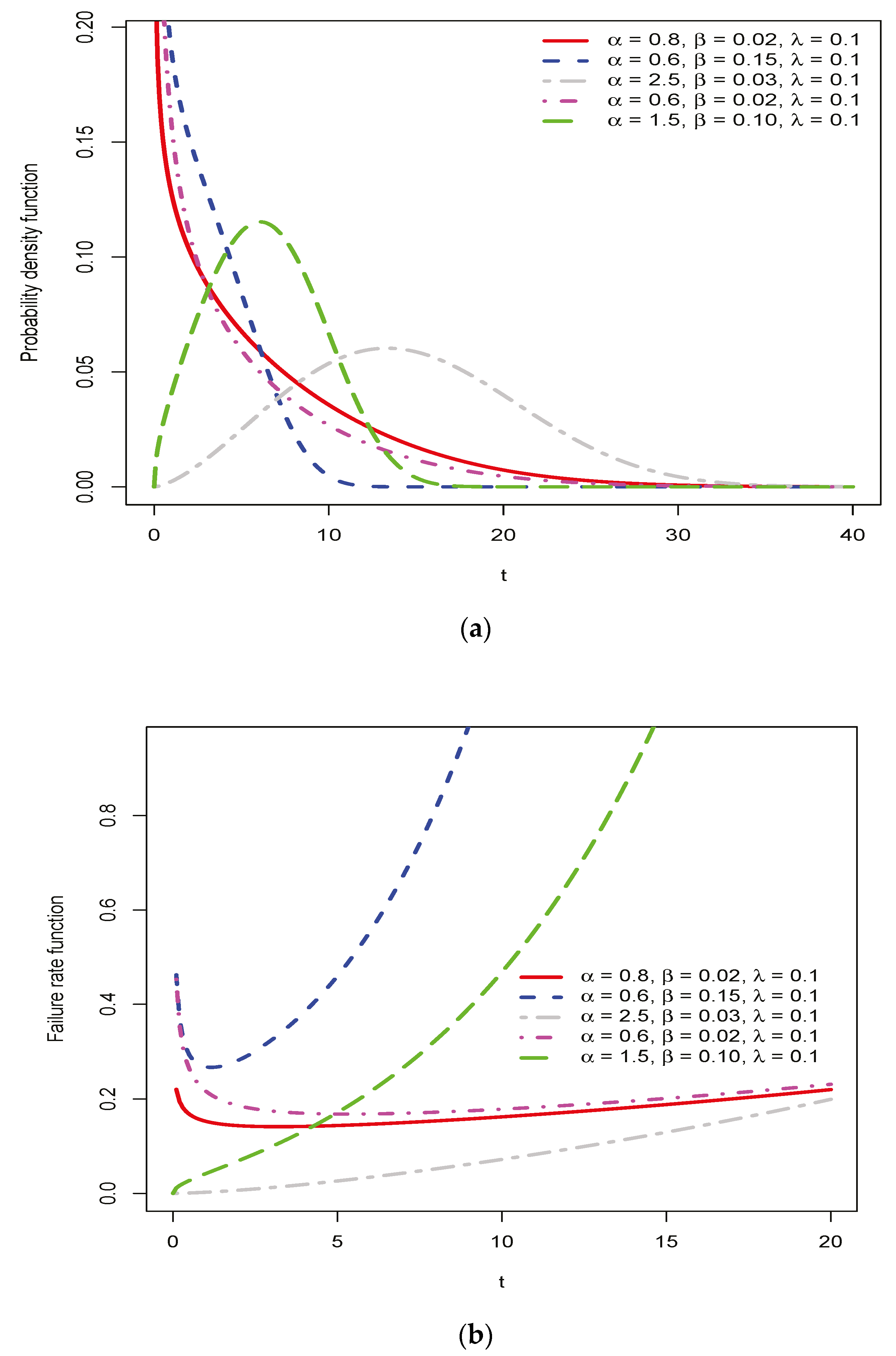
2. Model Formulation

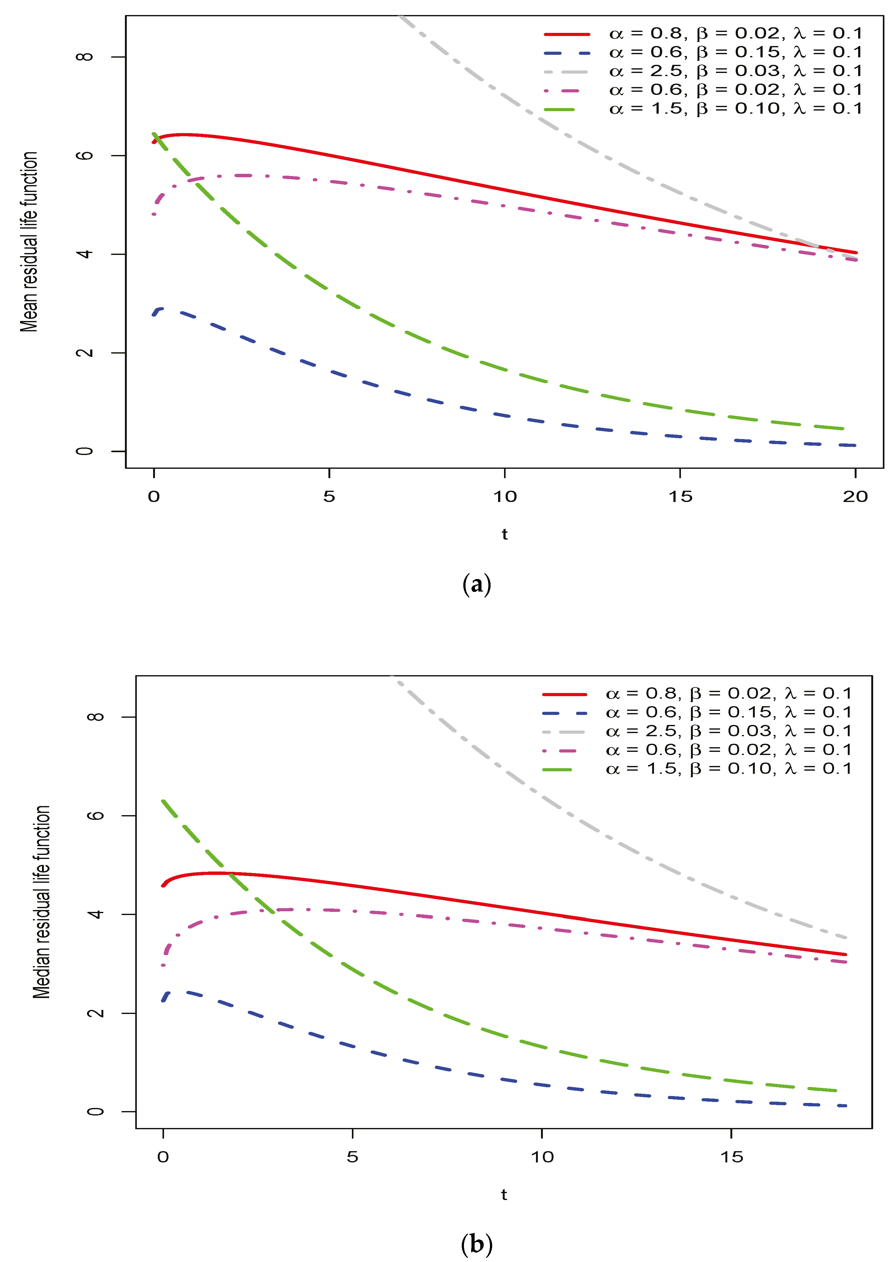
The gamma model is known by the probability distribution function (PDF)

$$f\left(t\right)=\frac{{\lambda }^{\alpha }}{\mathsf{\Gamma }\left(\alpha \right)}{t}^{\alpha -1}{e}^{-\lambda t},\alpha >0,\lambda >0,t\ge 0,$$

(1)

where $\alpha$ and $\lambda$ are shape and rate parameters, respectively.

The new modified gamma model $MG\left(\alpha ,\beta ,\lambda \right)$ can be characterized by the reliability function

$$R\left(t\right)=\frac{\mathsf{\Gamma }\left(\alpha ,\lambda t{e}^{\beta t}\right)}{\mathsf{\Gamma }\left(\alpha \right)},\alpha >0,\lambda >0,\beta >0, t\ge 0,$$

(2)

where $\mathsf{\Gamma }\left(\alpha ,x\right)={{\displaystyle \int }}_x^{\infty }{y}^{\alpha -1}{e}^{-y}dy$ shows the upper incomplete gamma function. The PDF of this model is

$$f\left(t\right)=\frac{1}{\mathsf{\Gamma }\left(\alpha \right)}{\lambda }^{\alpha }{t}^{\alpha -1}{e}^{\alpha \beta t}{e}^{-\lambda t{e}^{\beta t}}\left(1+\beta t\right),\alpha >0,\lambda >0,\beta >0, t\ge 0.$$

(3)

This model reduces to the gamma model when $\beta =0$. For $\alpha =1$. It is a special case of the modified Weibull model defined by Lai et al. [19]. As for the shape of the PDF, as shown in Figure 1a, it shows a decreasing and unimodal shape. The coefficient $e^{\beta t}$ ensures that the reliability function falls below the reliability of the baseline gamma distribution. If an object’s lifetime or life regularly follows the gamma model, it is exposed to a risk that increases with time under certain conditions. Such conditions may be the survival times of patients with serious diseases in which the disease progresses over time.

Figure 1. The PDF (a) and the FR function (b) of the MG model for some parameters.

The proposed MG model has a light right tail, and, in comparison with the gamma distribution, we have

$$\underset{t\to \infty }{\lim }\frac{R\left(t\right)}{R_G\left(t\right)}=\underset{t\to \infty }{\lim }\frac{{{\displaystyle \int }}_{\lambda t{e}^{\beta t}}^{\infty }{y}^{\alpha -1}{e}^{-y}dy}{{{\displaystyle \int }}_{\lambda t}^{\infty }{y}^{\alpha -1}{e}^{-y}dy}=\underset{t\to \infty }{\lim }{e}^{\alpha \beta t}{e}^{\lambda t\left(1-e^{\beta t}\right)}\left(1+\beta t\right)=0,$$

where $R\left(t\right)$ and $R_G\left(t\right)$ are the reliability functions of the MG and baseline gamma distributions, respectively. Thus, the MG model could properly fit to data with light right tail.

The $k$th moment of a random variable $T$ from $MG\left(\alpha ,\beta ,\lambda \right)$ is

$$\begin{array}{ll}E\left(T^k\right)\hfill & ={{\displaystyle \int }}_0^{\infty }k{t}^{k-1}R\left(t\right)dt=\frac{1}{\mathsf{\Gamma }\left(\alpha \right)}{{\displaystyle \int }}_0^{\infty }k{t}^{k-1}{{\displaystyle \int }}_{\lambda t{e}^{\beta t}}^{\infty }{y}^{\alpha -1}{e}^{-y}dydt\hfill \\ \hfill & =\frac{1}{\mathsf{\Gamma }\left(\alpha \right)}{{\displaystyle \int }}_0^{\infty }{y}^{\alpha -1}{e}^{-y}{(g^{-1}\left(y\right))}^{k}dy<\frac{1}{\mathsf{\Gamma }\left(\alpha \right){\lambda }^k}{{\displaystyle \int }}_0^{\infty }{y}^{\alpha +k-1}{e}^{-y}dy\hfill \\ \hfill & =E\left(X^k\right),\hfill \end{array}$$

(4)

where $X$ follows from $G\left(\alpha ,\lambda \right)$. The function $g$ is defined by $g\left(t\right)=\lambda t{e}^{\beta t}$, $t\ge 0$, and $g^{-1}$ is its inverse. The last inequality follows from the fact that $g^{-1}\left(y\right)<{\left(\frac{y}{\lambda }\right)}^k$. Thus, since the moments of the gamma distribution are finite, the moments of the MG distribution are also finite.

Figure 1 below shows various forms of densities at (a), including symmetric, asymmetric, unimodal, and reversed-J shapes. At (b), the FR function accommodates increasing or bathtub-shaped forms.

The $p$th quantile function $q\left(p\right)$, which determines the point $t_0$ for which $F\left(t_0\right)=p$ holds, can be computed numerically by solving the following equation as a function of $t$:

$$\mathsf{\Gamma }\left(\alpha ,\lambda t{e}^{\beta t}\right)=\left(1-p\right)\mathsf{\Gamma }\left(\alpha \right).$$

(5)

Dynamic Measures

There are many characterizations of the various lifespan distributions in the literature. These characterizations are essential because they offer new insights into the meaning of reliability features. For a random event at time $T$, the failure rate (FR) function at time $t$ indicates the instantaneous risk for the occurrence of the event and is mathematically defined by

$$r\left(t\right)=\frac{f\left(t\right)}{R\left(t\right)},t\ge 0,$$

which for $MG\left(\alpha ,\beta ,\lambda \right)$ simplifies to

$$r\left(t\right)=\frac{{\lambda }^{\alpha }{t}^{\alpha -1}{e}^{\alpha \beta t-\lambda t{e}^{\beta t}}\left(1+\beta t\right)}{\mathsf{\Gamma }\left(\alpha ,\lambda t{e}^{\beta t}\right)},\hspace{1em}t\ge 0.$$

The function of the mean residual life (MRL) of a random life $T$ at time $t$ represents the conditional remaining lifetime, given it has been survived until $t$, i.e.,

$$m\left(t\right)=E\left(T-t|T>t\right)=\frac{{{\displaystyle \int }}_t^{\infty }R\left(x\right)dx}{R\left(t\right)}=\frac{{{\displaystyle \int }}_t^{\infty }\mathsf{\Gamma }\left(\alpha ,\lambda x{e}^{\beta x}\right)dx}{\mathsf{\Gamma }\left(\alpha ,\lambda t{e}^{\beta t}\right)}.\hspace{1em}t\ge 0.$$

It could not be simplified further and should be computed numerically.

Similarly, the p-quantile residual life (p-QRL) function of a random life $T$ at time $t$ gives the pth quantile of its conditional residual life if it has survived to t and is formally written as follows:

$$q_p\left(t\right)=q\left(p|T>t\right)=R^{-1}\left(\overline{p}R\left(t\right)\right)-t,\hspace{1em}t\ge 0.$$

(6)

The special case $p=0.5$ is called the median residual life function and is a good alternative to the MRL function. Figure 2 shows the MRL and median residual life functions for some parameters and has decreasing and unimodal forms.

Figure 2. The MRL (a) and the median residual life (b) functions of MG model for some parameters.

As a valuable tool to develop different properties of models, stochastic orders by quantifying the concept of one random variable being more significant than another are considered. These, however, are partial orders, thus one random variable X may be neither stochastically greater than, less than, nor equal to another random variable Y. Many different orders have various applications, as per Lai and Xie [20]. The following results show that the MG distribution is ordered under the right conditions concerning the usual stochastic and failure rate orders.

Proposition 1.

Let$T_1\sim MG\left(\alpha ,{\beta }_1,\lambda \right)$, $T_2\sim MG\left(\alpha ,{\beta }_2,\lambda \right)$, and${\beta }_1<{\beta }_2$. Then,$T_2<T_1$in stochastic ordering.

Proof. 

Suppose that $R_1$ and $R_2$ represent the reliability functions of $T_1$ and $T_2$, respectively. Following the definition of stochastic order (see Lai and Xie [20]), we should show that $R_1\left(t\right)\ge R_2\left(t\right)$ for all $t\ge 0,$ which is clear. □

Specially, if $T_1\sim G\left(\alpha ,\lambda \right)$ and $T_2\sim MG\left(\alpha ,\beta ,\lambda \right)$, then $T_2<T_1$ in stochastic ordering.

Proposition 2.

Let$\alpha \ge 1$,$T_1\sim MG\left(\alpha ,{\beta }_1,\lambda \right)$, $T_2\sim MG\left(\alpha ,{\beta }_2,\lambda \right)$, and${\beta }_1<{\beta }_2$. Then, $T_2<T_1$in FR ordering.

Proof. 

Suppose that $R_1$ and $R_2$ are the reliability functions of $T_1$ and $T_2$, respectively. Following the definition of FR order (see Lai and Xie [20]), we should show that the following expression is increasing for all $t\ge 0$:

$$\eta \left(t\right)=\frac{R_1\left(t\right)}{R_2\left(t\right)}=\frac{{{\displaystyle \int }}_{\lambda t{e}^{{\beta }_{1}t}}^{\infty }{y}^{\alpha -1}{e}^{-y}dy}{{{\displaystyle \int }}_{\lambda t{e}^{{\beta }_{2}t}}^{\infty }{y}^{\alpha -1}{e}^{-y}dy}.$$

To reduce the complexity of differentiation, take $l_i=\lambda t{e}^{{\beta }_{i}t}$ and $i=1,2$. Thus

$$\eta \left(t\right)=\frac{{{\displaystyle \int }}_{l_1\left(t\right)}^{\infty }{y}^{\alpha -1}{e}^{-y}dy}{{{\displaystyle \int }}_{l_2\left(t\right)}^{\infty }{y}^{\alpha -1}{e}^{-y}dy}.$$

By differentiating $\eta$ with respect to $t$, it can be verified that the sign of ${\eta }^{\prime }\left(t\right)$ is the same as the sign of the following expression, where $l_i$ represents $l_i\left(t\right)$ for simplicity.

$$\begin{array}{ll}{\eta }^{\prime }\left(t\right)\hfill & \propto {l^{\prime }}_2\left(t\right)l_2^{\alpha -1}{e}^{-l_2}{{\displaystyle \int }}_{l_1}^{\infty }{y}^{\alpha -1}{e}^{-y}dy-{l^{\prime }}_1\left(t\right)l_1^{\alpha -1}{e}^{-l_1}{{\displaystyle \int }}_{l_2}^{\infty }{y}^{\alpha -1}{e}^{-y}dy\hfill \\ \hfill & ={l^{\prime }}_2\left(t\right){{\displaystyle \int }}_{l_1}^{\infty }{(l_{2}y)}^{\alpha -1}{e}^{-\left(y+l_2\right)}dy-{l^{\prime }}_1\left(t\right){{\displaystyle \int }}_{l_2}^{\infty }{(l_{1}y)}^{\alpha -1}{e}^{-\left(y+l_1\right)}dy\ge 0,\hfill \end{array}$$

(7)

since ${l^{\prime }}_1\left(t\right)<{l^{\prime }}_2\left(t\right)$ and $\alpha \ge 1$

$${{\displaystyle \int }}_{l_1}^{\infty }{(l_{2}y)}^{\alpha -1}{e}^{-\left(y+l_2\right)}dy\ge {{\displaystyle \int }}_{l_2}^{\infty }{(l_{1}y)}^{\alpha -1}{e}^{-\left(y+l_1\right)}dy.$$

Thus, by $\left(7\right)$, $\eta \left(t\right)$ is increasing and, consequently, $T_2<T_1$ in FR ordering. □

As a direct consequence of Proposition 2, and with the assumptions of this proposition, we can write that $T_2<T_1$ in MRL and $p$-QRL orderings (see Lai and Xie [20]).

3. Parameters Estimation

Parameters estimation is essential in machine learning, statistics, communication systems, radar, and many other fields. Suppose we have an ordered independent and identically distributed realization $t_1\le t_2\le \dots \le t_n$ of $MG\left(\alpha ,\beta ,\lambda \right)$. In this section, we discuss some methods for estimating the parameters.

3.1. Maximum Likelihood Method

Model parameters are estimated using the MG distribution’s maximum likelihood estimators (MLEs). The log–likelihood function corresponding to the MG model is

$$l\left(\alpha ,\beta ,\lambda ;t\right)=-n\ln \mathsf{\Gamma }\left(\alpha \right)+n\alpha \ln \lambda +\left(\alpha -1\right){\displaystyle \sum }_{i=1}^n\ln t_i+\alpha \beta {\displaystyle \sum }_{i=1}^n{t}_i+{\displaystyle \sum }_{i=1}^n\ln \left(1+\beta t_i\right)-\lambda {\displaystyle \sum }_{i=1}^n{t}_i{e}^{\beta t_i}.$$

(8)

To estimate the parameters, we can maximize the log–likelihood function with respect to $\left(\alpha ,\beta ,\lambda \right)$. In another approach, the answer to the following log–likelihood equations can be considered as maximum likelihood (ML) estimation.

$$\frac{\partial }{\partial \alpha }l\left(\alpha ,\beta ,\lambda ;t\right)=-n\frac{{\mathsf{\Gamma }}^{\prime }\left(\alpha \right)}{\mathsf{\Gamma }\left(\alpha \right)}+n\ln \lambda +{\displaystyle \sum }_{i=1}^n\ln t_i+\beta {\displaystyle \sum }_{i=1}^n{t}_i=0,$$

$$\frac{\partial }{\partial \beta }l\left(\alpha ,\beta ,\lambda ;t\right)=\alpha {\displaystyle \sum }_{i=1}^n{t}_i+{\displaystyle \sum }_{i=1}^n\frac{t_i}{1+\beta t_i}-\lambda {\displaystyle \sum }_{i=1}^n{t}_i^2{e}^{\beta t_i}=0,$$

and

$$\frac{\partial }{\partial \lambda }l\left(\alpha ,\beta ,\lambda ;t\right)=\frac{n\alpha }{\lambda }-{\displaystyle \sum }_{i=1}^n{t}_i{e}^{\beta t_i}=0.$$

To approximate the asymptotic variance of the maximum likelihood estimator (MLE), we can calculate the observed Fisher information matrix to be $\left(\widehat{\alpha },\widehat{\beta },\widehat{\lambda }\right)$

$$M=\left[\begin{array}{lll}-\frac{{\partial }^2}{\partial {\alpha }^2}\hfill & -\frac{{\partial }^2}{\partial \alpha \partial \beta }\hfill & -\frac{{\partial }^2}{\partial \alpha \partial \lambda }\hfill \\ -\frac{{\partial }^2}{\partial \beta \partial \alpha }\hfill & -\frac{{\partial }^2}{\partial {\beta }^2}\hfill & -\frac{{\partial }^2}{\partial \beta \partial \lambda }\hfill \\ -\frac{{\partial }^2}{\partial \lambda \partial \alpha }\hfill & -\frac{{\partial }^2}{\partial \lambda \partial \beta }\hfill & -\frac{{\partial }^2}{\partial {\lambda }^2}\hfill \end{array}\right]l\left(\alpha ,\beta ,\lambda ;t\right).$$

(9)

Then, $\left(\widehat{\alpha }-\alpha ,\widehat{\beta }-\beta ,\widehat{\lambda }-\lambda \right)$ converges weakly to the multivariate normal $N\left(0,M^{-1}\right).$ Therefore, approximate confidence intervals for the MLE can be calculated using the inverse of the observed information matrix and the standard normal quantiles.

3.2. Least Squared Error Method

In the least squared error (LSE) approach to estimate the parameters, we should minimize the sum of squared distances between the estimated distribution function and the empirical distribution function, i.e., the following expression should be minimized.

$$S^2={\displaystyle \sum }_{i=1}^n{(F\left(t_i\right)-\widehat{F}\left(t_i\right))}^2,$$

which can be simplified to

$$S^2={\displaystyle \sum }_{i=1}^n{\left(\frac{\mathsf{\Gamma }\left(\alpha ,\lambda t_i{e}^{\beta t_i}\right)}{\mathsf{\Gamma }\left(\alpha \right)}-\frac{n-i}{n}\right)}^2.$$

Thus, the LSE estimates are computed by

$$\left(\widehat{\alpha },\widehat{\beta },\widehat{\lambda }\right)=\arg \underset{(\alpha >0,\beta >0,\lambda >0)}{\min }{\displaystyle \sum }_{i=1}^n{\left(\frac{\mathsf{\Gamma }\left(\alpha ,\lambda t_i{e}^{\beta t_i}\right)}{\mathsf{\Gamma }\left(\alpha \right)}-\frac{n-i}{n}\right)}^2.$$

3.3. Anderson-Darling Method

In the Anderson–Darling (AD) method, a weighted sum of the squares of the distances between the estimated distribution function and the empirical distribution function is minimized. The proper weights are $\frac{1}{F\left(t_i\right)\left(1-F\left(t_i\right)\right)}$. Thus, the estimate could be obtained as in the following.

$$\left(\widehat{\alpha },\widehat{\beta },\widehat{\lambda }\right)=\arg \underset{(\alpha >0,\beta >0,\lambda >0)}{\min }{\displaystyle \sum }_{i=1}^n\frac{1}{F\left(t_i\right)\left(1-F\left(t_i\right)\right)}{(\frac{\mathsf{\Gamma }\left(\alpha ,\lambda t_i{e}^{\beta t_i}\right)}{\mathsf{\Gamma }\left(\alpha \right)}-\frac{n-i}{n})}^2.$$

3.4. Quantile Based Method

The quantile-based (QB) method considers the distances between the quantiles of the estimated model and the empirical quantiles of the data. Thus, the QB estimate of the parameters is

$$\left(\widehat{\alpha },\widehat{\beta },\widehat{\lambda }\right)=\arg \underset{(\alpha >0,\beta >0,\lambda >0)}{\min }{\displaystyle \sum }_{i=1}^n{\left(q\left(\frac{i}{n}\right)-t_i\right)}^2,$$

where the quantile function $q$ is defined by (5).

4. Investigation of the Estimator’s Behavior

The efficiency and consistency of the discussed estimators of the parameters are investigated by simulations. To generate an instance $T$ of $MG\left(\alpha ,\beta ,\lambda \right)$, we solve the following equation:

$$\frac{\mathsf{\Gamma }\left(\alpha ,\lambda T\right)}{\mathsf{\Gamma }\left(\alpha \right)}=U,$$

(10)

where $U$ is a random instance of the standard uniform model.

In each run, $r=1000$ replicates of samples of size $n=80$ or $150$ from MG are simulated with selected parameters. Then, the parameters for each sample are estimated using ML, LSE, AD, or QB methods. The optimizations are performed using the built-in function “optim” or the programming language R for all methods. The initial values needed for the optimization are chosen randomly from a uniform distribution, for example, for α on the interval $\left(0.9\alpha ,1.1\alpha \right)$ and similarly for $\beta$ and $\lambda$. Table 1 shows the bias (B) and mean square error (MSE) of the ML and QB estimators for all parameters. Similarly, Table 2 shows the results for the LSE and AD estimators. From these tables, the following observations can be made.

Table 1. Simulation results for methods ML and QB. The first, second, and third lines of each cell refer to $\alpha$, $\beta$, and $\lambda$, respectively.

		$\mathit{n}$
Method	$\mathit{\alpha }, \mathit{\beta }, \mathit{\lambda }$	80		150
		B	MSE	B	MSE
ML	1.1, 0.01, 0.1	0.0086	0.04794	0.0054	0.02583
		0.0046	0.00017	0.0021	0.00007
		−0.0009	0.00125	0.0003	0.00072
	1, 0.1, 0.05	0.0681	0.10696	0.0219	0.04698
		0.0051	0.00191	0.0045	0.00093
		0.0120	0.00212	0.0044	0.00079
	2, 0.5, 0.01	0.7002	5.2393	0.3272	1.76903
		0.0495	0.06745	0.02533	0.03287
		0.05366	0.02518	0.0201	0.00395
QB	1.1, 0.01, 0.1	−0.0014	0.00492	0.0002	0.00403
		−0.000013	$3.44\times {10}^{-7}$	$2.11\times {10}^{-6}$	$3.336\times {10}^{-7}$
		−0.00012	$3.54\times {10}^{-5}$	$2.09\times {10}^{-5}$	$3.335\times {10}^{-5}$
	1, 0.1, 0.05	−0.0039	0.00328	−0.0021	0.00032
		−0.00038	$3.28\times {10}^{-5}$	−0.0002	$3.12\times {10}^{-5}$
		−0.00020	$8.21\times {10}^{-6}$	−0.00010	$8.01\times {10}^{-6}$
	2, 0.5, 0.01	−0.0054	0.01338	0.0009	0.01311
		−0.0014	0.00087	0.00024	0.00081
		$2.74\times {10}^{-5}$	$3.64\times {10}^{-7}$	$4.77\times {10}^{-6}$	$3.43\times {10}^{-7}$

Table 2. Simulation results for the methods LSE and AD. The first, second, and third lines of each cell refer to $\alpha$, $\beta$, and $\lambda$, respectively.

		$\mathit{n}$
Method	$\mathit{\alpha }, \mathit{\beta }, \mathit{\lambda }$	80		150
		B	MSE	B	MSE
LSE	1.1, 0.01, 0.1	−0.0475	0.0705	−0.0190	0.03801
		0.0091	0.00051	0.0044	0.00020
		−0.0052	0.00193	−0.0020	0.00110
	1, 0.1, 0.05	0.01710	0.16723	0.0089	0.09612
		0.0204	0.00534	0.0123	0.00241
		0.0117	0.00363	0.0064	0.00189
	2, 0.5, 0.01	0.1615	0.92601	0.1485	0.65873
		0.0299	0.02355	0.0167	0.01754
		0.0112	0.00104	0.0089	0.00064
AD	1.1, 0.01, 0.1	−0.0870	0.05139	−0.0458	0.02675
		0.0079	0.00030	0.0042	0.00013
		−0.0113	0.00132	−0.0062	0.00078
	1, 0.1, 0.05	−0.0867	0.08498	−0.0474	0.04829
		0.0266	0.00348	0.0133	0.00138
		−0.0042	0.00133	−0.00211	0.00079
	2, 0.5, 0.01	−0.1091	0.85380	−0.0697	0.59151
		0.0794	0.03572	0.0540	0.02315
		0.0074	0.00112	0.0052	0.00058

• All estimators are consistent and efficient for estimating the model parameters.
• The AD estimator, a weighted form of the LSE method, outperforms the LSE estimator.
• The QB estimator has a very small MSE but does not improve significantly with sample size.

5. Applications

In this section, we present two applications with real data to demonstrate the MG model’s flexibility empirically.

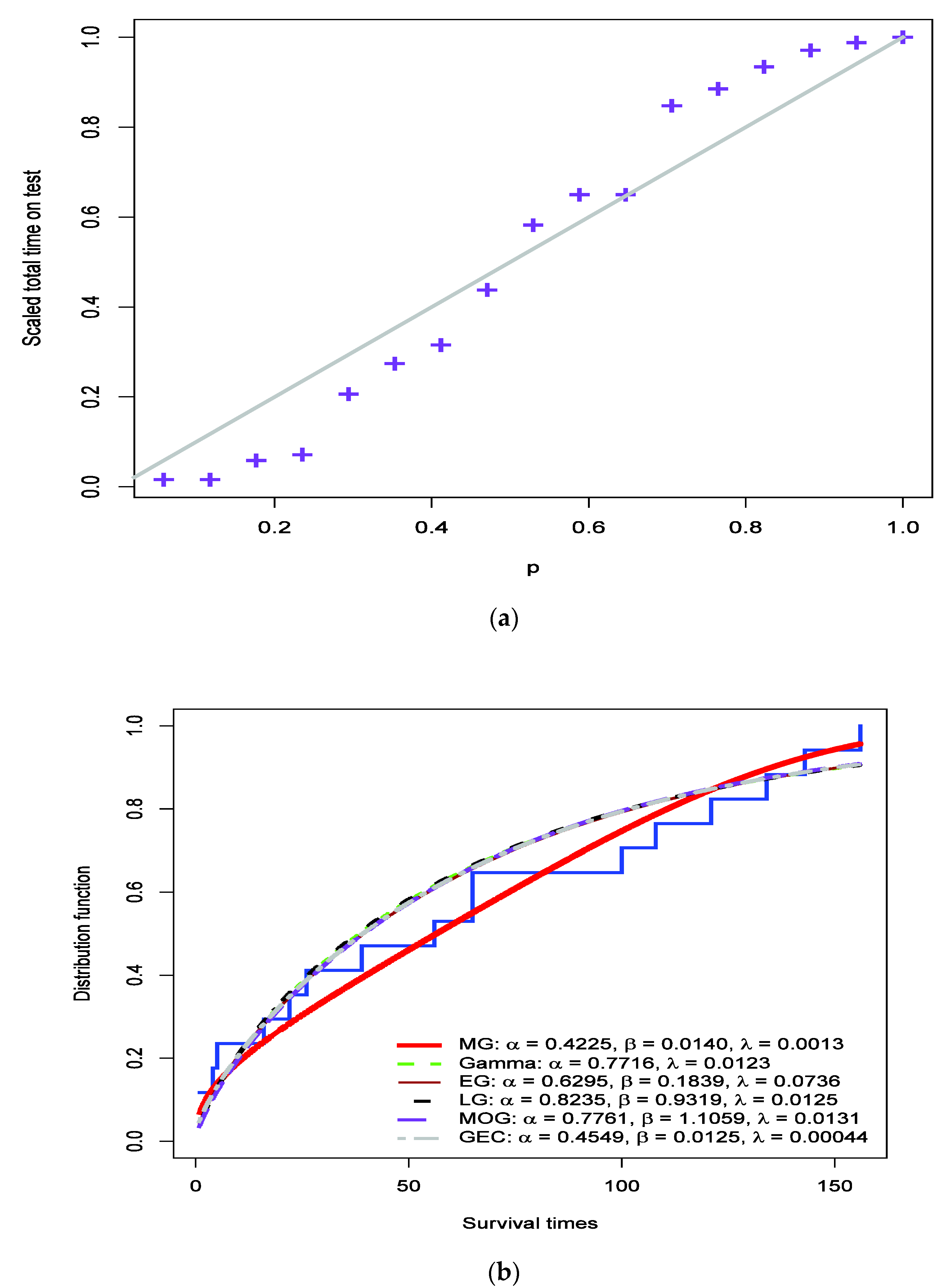
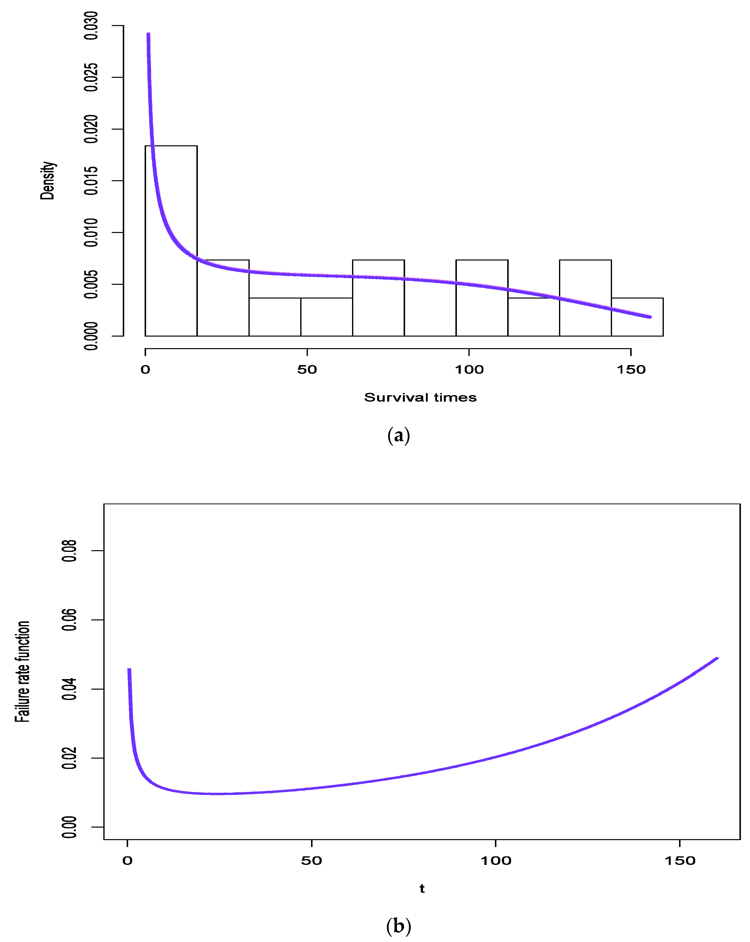
5.1. Application 1 Survival Times of AG Positive Patients Data

Table 3 shows 17 survival times in weeks for a group of patients who died from acute myelogenous leukemia. These patients are designated as AG positive, meaning that they are identified by the presence of Auer rods and significant granulation of leukemic cells in the bone marrow at diagnosis. For more details on this dataset and patient specifications, see Feigl and Zelen [21].

Table 3. Survival times (weeks) of a group of AG positive patients.

65	156	100	134	16	108	121	4	39	143
56	26	22	1	1	5	65

In a comparative analysis, the alternative distributions gamma, Lehmann gamma (LG), exponentiated gamma (EG), Marshal–Olkin gamma (MOG), and gamma-exponential-competitive-risk (GEC) models, respectively, with the following reliability functions are considered.

$$R\left(t\right)=\frac{\mathsf{\Gamma }\left(\alpha ,\lambda t\right)}{\mathsf{\Gamma }\left(\alpha \right)},\alpha >0,\lambda >0,t\ge 0,$$

$$R\left(t\right)=1-{(1-\frac{\mathsf{\Gamma }\left(\alpha ,\lambda t\right)}{\mathsf{\Gamma }\left(\alpha \right)})}^{\beta },\alpha >0,\lambda >0,\beta >0,t\ge 0,$$

$$R\left(t\right)={(\frac{\mathsf{\Gamma }\left(\alpha ,\lambda t\right)}{\mathsf{\Gamma }\left(\alpha \right)})}^{\beta },\alpha >0,\beta >0,\lambda >0,t\ge 0,$$

$$R\left(t\right)=\frac{\beta \mathsf{\Gamma }\left(\alpha ,\lambda t\right)}{\mathsf{\Gamma }\left(\alpha \right)-\overline{\beta }\mathsf{\Gamma }\left(\alpha ,\lambda t\right)},\alpha >0,\beta >0,\lambda >0,t\ge 0,$$

and

$$R\left(t\right)=\frac{\mathsf{\Gamma }\left(\alpha ,\lambda t\right)}{\mathsf{\Gamma }\left(\alpha \right)}{e}^{-\beta t},\alpha >0,\beta >0,\lambda >0,t\ge 0,$$

where $\overline{\beta }=1-\beta$. Then, the parameters of all models are estimated using the ML method. The results of the analysis are summarized in Table 4. Indicated are the Akaike information criterion (AIC), Bayesian information criterion (BIC), the Kolmogorov–Smirnov (KS) statistic, the Cramer-von Mises (CVM) statistic, and the Anderson–Darling (AD) statistic, as well as the corresponding p-values. Based on these benchmarks, MG performs significantly better than the other candidates. Figure 3 shows the Total Time on Test (TTT) plot indicating a bathtub-shaped FR function for this dataset. This plot shows the empirical and the fitted CDF for the selected models, which graphically confirms that the MG model provides a better fit than the other models considered. Figure 4 shows the estimated PDF and FR functions for the MG model. It provides a bathtub-shaped FR function and a decreasing shape for PDF.

Table 4. Results of fitting the MG distribution and some alternatives to survival times data.

Model	$\widehat{\mathit{\alpha }}$	$\widehat{\mathit{\beta }}$	$\widehat{\mathit{\lambda }}$	AIC	BIC	K-S p-Value	CVM p-Value	AD p-Value
MG	0.4225	0.0140	0.0013	175.67	178.17	0.1015 0.9948	0.0384 0.9459	0.2695 0.9588
Gamma	0.7716	—	0.0123	177.74	179.41	0.1464 0.8591	0.0758 0.7229	0.5217 0.7223
LG	0.8235	0.9319	0.0125	179.72	182.22	0.1466 0.8584	0.0785 0.7227	0.5197 0.7243
EG	0.6295	0.1839	0.0736	179.54	182.04	0.1437 0.8739	0.0678 0.7717	0.4690 0.7763
MOG	0.7761	1.1059	0.0131	179.61	182.11	0.1457 0.8630	0.0720 0.7458	0.5186 0.7254
GEC	0.4549	0.0125	0.00044	179.81	182.31	0.1444 0.8705	0.0680 0.7704	0.4658 0.7795

Figure 3. (a): The TTT representation of the survival times data. (b): The empirical and adjusted CDF to MG and alternative models for this data set.

Figure 4. The PDF (a) and the FR function (b) of the fitted MG model for survival times data.

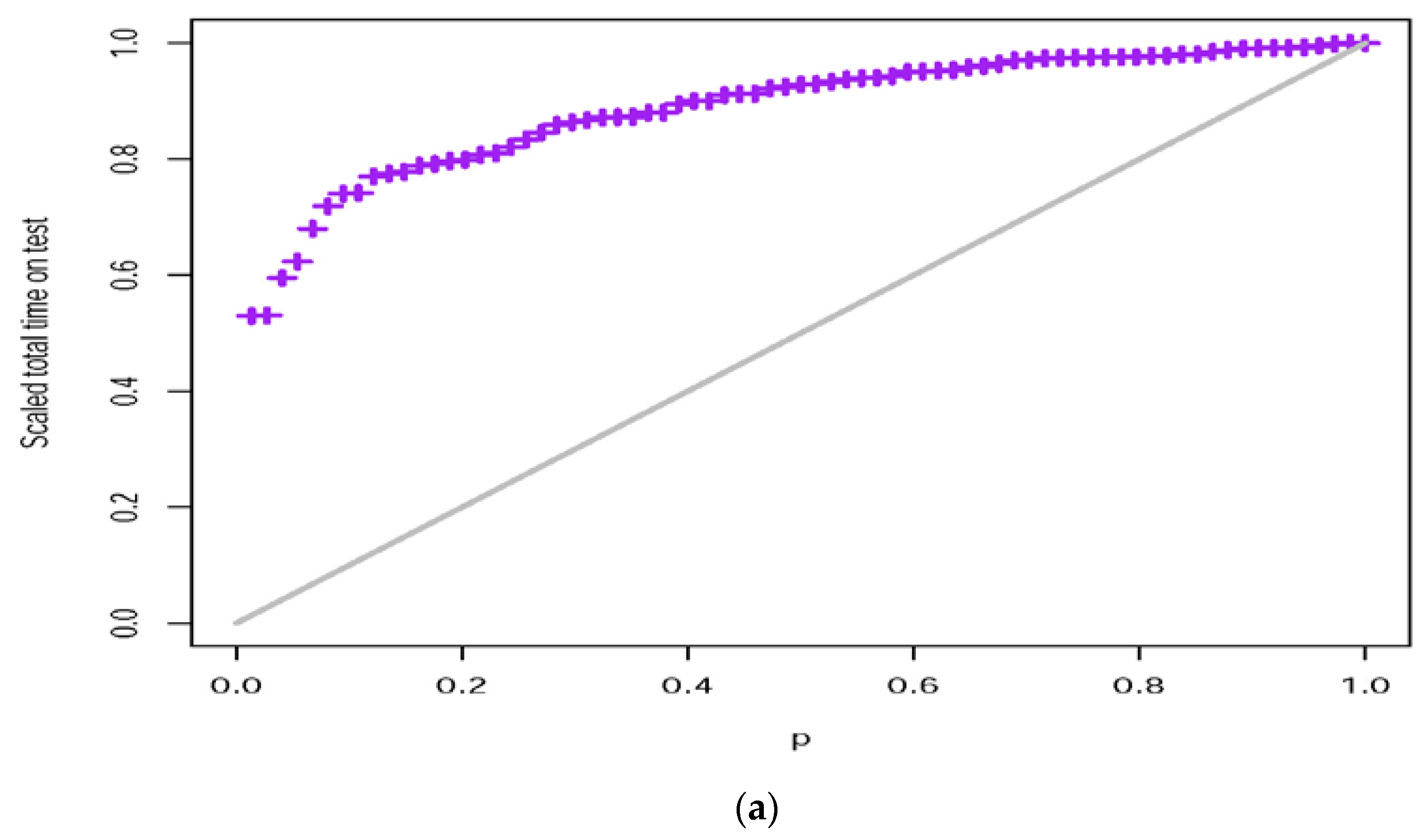
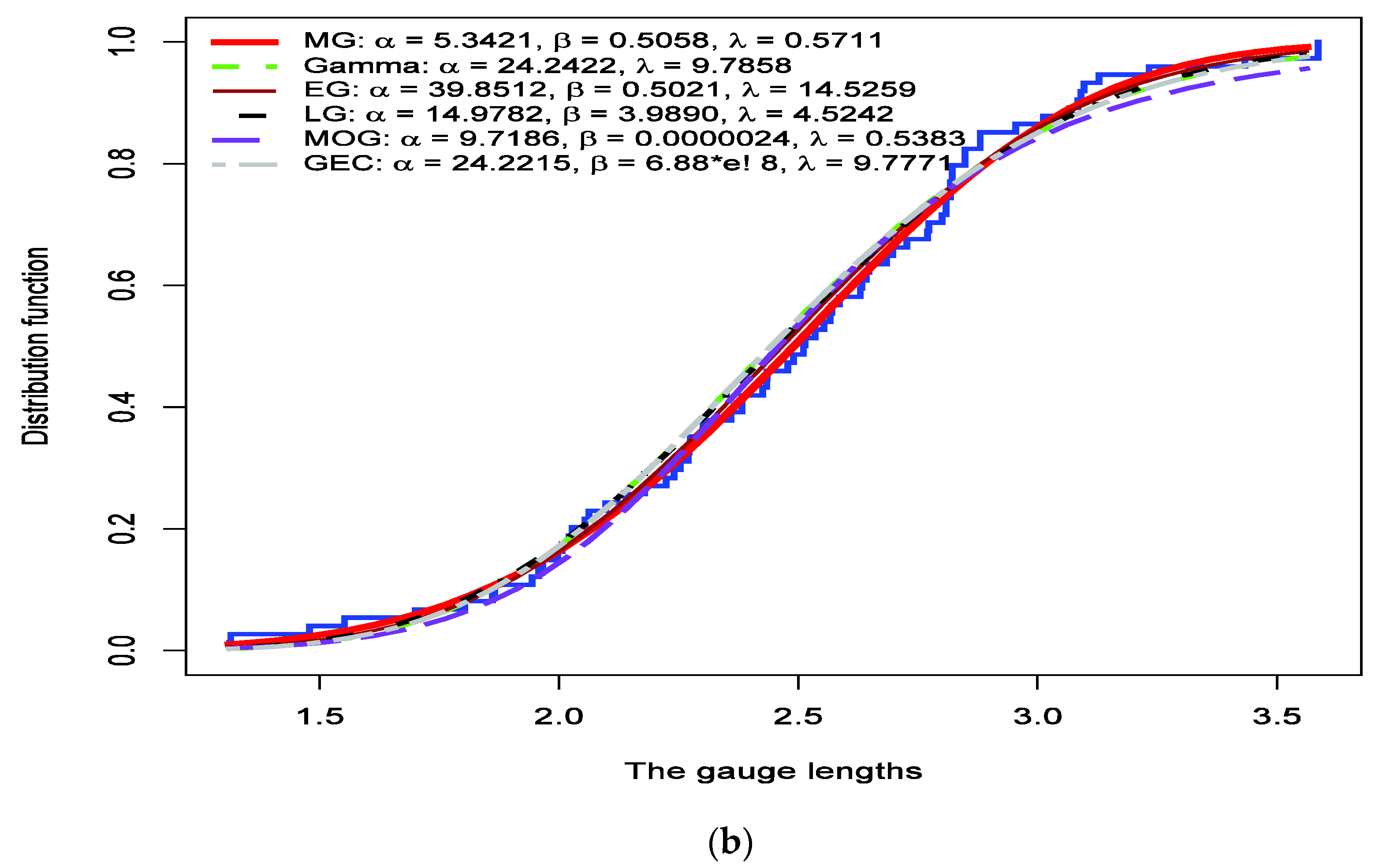
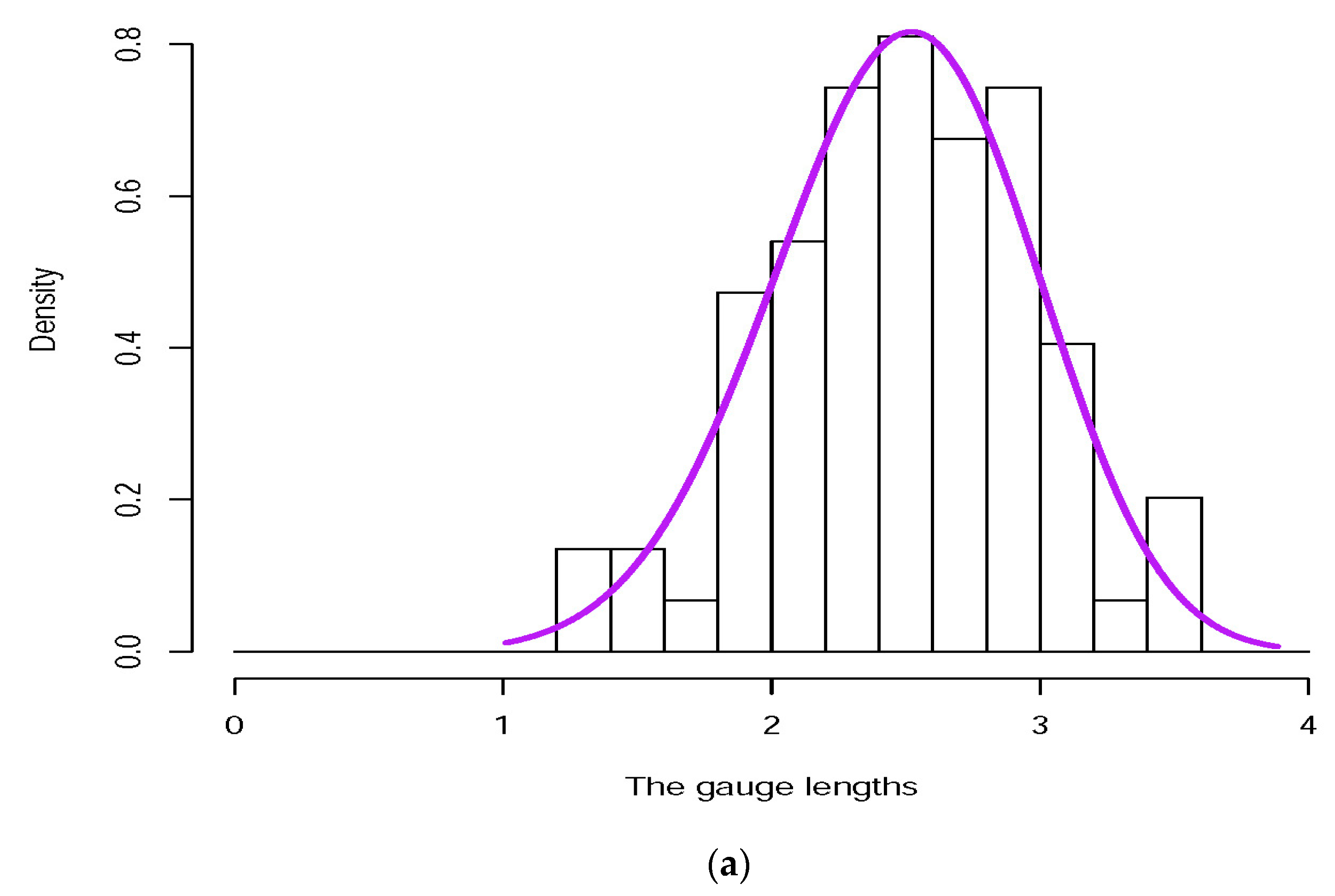
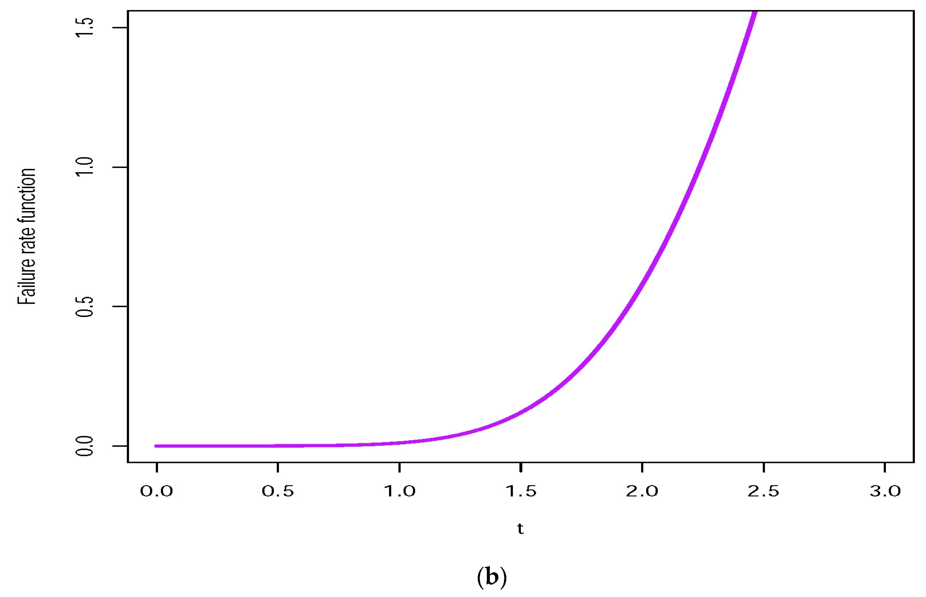
5.2. Application 2 The Gauge Lengths Data

Table 5 reports 74 observations of the gauge lengths of 20 mm. The data set was previously studied by Alfaer et al. [22] and Ahmed et al. [23].

Table 5. The gauge lengths of 20 mm.

1.312	1.314	1.479	1.552	1.700	1.803	1.861	1.865	1.944	1.958
1.966	1.997	2.006	2.021	2.027	2.055	2.063	2.098	2.140	2.179
2.224	2.240	2.253	2.270	2.272	2.274	2.301	2.301	2.359	2.382
2.426	2.434	2.435	2.382	2.478	2.554	2.514	2.511	2.490	2.535
2.566	2.570	2.586	2.629	2.800	2.773	2.770	2.809	3.585	2.818
2.642	2.726	2.697	2.684	2.648	2.633	3.128	3.090	3.096	3.233
2.821	2.880	2.848	2.818	3.067	2.821	2.954	2.809	3.585	3.084
3.012	2.880	2.848	3.433

The parameters of the MG model and all alternatives considered in the previous example are estimated by the ML method. The results of the analysis are included in Table 6.

Table 6. Results of fitting the MG distribution and some alternatives to gauge lengths data.

Model	$\widehat{\mathbf{\alpha }}$	$\widehat{\mathbf{\beta }}$	$\widehat{\mathbf{\lambda }}$	AIC	BIC	K-S p-Value	CVM p-Value	AD p-Value
MG	5.3421	0.5058	0.5711	108.34	115.25	0.0582 0.9632	0.0265 0.9866	0.2087 0.9878
Gamma	24.2422	—	9.7858	110.33	114.94	0.0681 0.8821	0.0864 0.6570	0.5642 0.6818
LG	39.8512	0.5021	14.5259	110.76	117.67	0.0619 0.9387	0.0726 0.7368	0.4633 0.7839
EG	14.9782	3.9890	4.5242	109.49	116.41	0.0557 0.9758	0.0474 0.8932	0.3246 0.9183
MOG	9.7186	0.0000024	0.5383	115.17	122.08	0.0631 0.9301	0.0767 0.7124	0.6256 0.6235
GEC	24.2215	6.88 × 10−8	9.7771	112.33	119.24	0.0680 0.8830	0.0863 0.6577	0.5639 0.6822

The AIC, BIC, KS, CVM, AD, as well as the corresponding p-values, are reported. Based on the results, the MG proves to be better than others. Figure 5a shows the TTT plot, which shows an increasing failure rate function. Figure 5b draws the empirical and fitted CDFs for the selected models and shows a very close competition for describing the data between selected models. Additionally, Figure 6 provides the estimated PDF and FR functions for the MG model.

Figure 5. (a): The TTT representation of the gauge lengths data. (b): The empirical and adjusted CDF to MG and alternative models for this data set.

Figure 6. The PDF (a) and the FR function (b) of the fitted MG model for gauge lengths data.

6. Conclusions

Statistical models play an essential role in survival analysis and the medical field. These models provide satisfactory results in modeling various types of data sets. In this paper, we have implemented a novel model to update the flexibility level of the existing models. A modified gamma model is introduced, and some basic properties are investigated. The FR function can be increasing or bathtub shaped. In addition, the MRL and p-QRL functions are studied. Four methods, ML, LSE, AD, and QB, to estimate the proposed model parameters are discussed. The simulation results show that these estimators are consistent and efficient. The results of the comparative analysis show that the proposed model is useful for modeling survival data. In general, the new model could be presented as a flexible and simple model for the analysis of survival data when the upper tail seems to be lighter than that of an ordinary gamma model (due to the increased risk in the occurrence of the event), and the data have a bathtub-shaped FR function. The results offer new concepts and applications in survival analysis, medical statistics, and risk theory. The new model will be beneficial to researchers in the future and will be considered a better choice over the baseline model. Further properties and applications of the new model may be considered in the future of this research. In particular, the following topics are exciting and remain open problems:

• Bayesian and E-Bayesian estimation based on complete and different censoring schemes;
• Proposing a bivariate family of this model to extend the univariate case.

References

- Petty, G.W.; Huang, W. The modified gamma size distribution applied to inhomogeneous and nonspherical particles: Key relationships and conversions. J. Atmos. Sci. 2011, 68, 1460–1473. [Google Scholar] [CrossRef]
- Belikov, A.V. The number of key carcinogenic events can be predicted from cancer incidence. Sci. Rep. 2017, 7, 12170. [Google Scholar] [CrossRef] [PubMed]
- Boland, P.J. Statistical and Probabilistic Methods in Actuarial Science; Chapman and Hall (CRC): Boca Raton, FL, USA, 2007. [Google Scholar]
- Aksoy, H. Use of gamma distribution in hydrological analysis. Turk. J. Eng. Environ. Sci. 2000, 24, 419–428. [Google Scholar]
- Wright, M.C.M.; Winter, I.M.; Forster, J.J.; Bleeck, S. Response to best-frequency tone bursts in the ventral cochlear nucleus is governed by ordered inter-spike interval statistics. Hear. Res. 2014, 317, 23–32. [Google Scholar] [CrossRef] [PubMed]
- Williams, M.M.R. On the modified gamma distribution for representing the size spectra of coagulating aerosol particles. J. Colloid Interface Sci. 1985, 103, 516–527. [Google Scholar] [CrossRef]
- Ong, J.T.; Shan, Y.Y. Modified gamma model for Singapore rain drop size distribution. IGARSS’97. In Proceedings of the 1997 IEEE International Geoscience and Remote Sensing Symposium Proceedings. Remote Sensing—A Scientific Vision for Sustainable Development, Singapore, 3–8 August 1997; Volume 4, pp. 1757–1759. [Google Scholar]
- Muralidharan, K.; Kale, B.K. Modified gamma distribution with singularity at zero. Commun. Stat.-Simul. Comput. 2002, 31, 143–158. [Google Scholar] [CrossRef]
- Gebrenegus, G. The extended generalized gamma model and its special cases: Applications to modeling marriage durations. Qual. Quant. 2005, 39, 71–85. [Google Scholar]
- Nadarajah, S.; Gupta, A.K. The exponentiated gamma distribution with application to drought data. Calcutta Stat. Assoc. Bull. 2007, 59, 29–54. [Google Scholar] [CrossRef]
- Shawky, A.I.; Bakoban, R.A. Exponentiated gamma distribution: Different methods of estimations. J. Appl. Math. 2012, 2012, 284296. [Google Scholar] [CrossRef]
- Cordeiro, G.M.; Lima, M.S.; Gomes, A.E. The gamma extended Weibull distribution. J. Stat. Distrib. Appl. 2016, 5, 1–19. [Google Scholar] [CrossRef]
- Feroze, N.; Elbatal, I. Beta exponentiated gamma distribution: Some properties and estimation. Pak. J. Stat. Oper. Res. 2016, 12, 141–154. [Google Scholar] [CrossRef][Green Version]
- Barriga, G.D.; Cordeiro, G.M.; Dey, D.K.; Cancho, V.G.; Louzada, F.; Suzuki, A.K. The Marshall-Olkin generalized gamma distribution. Commun. Stat. Appl. Methods 2018, 25, 245–261. [Google Scholar] [CrossRef]
- Marshall, A.W.; Olkin, I. A new method for adding a parameter to a family of distributions with application to the exponential and Weibull families. Biometrika 1997, 84, 641–652. [Google Scholar] [CrossRef]
- Mead, M.; Nassar, M.M.; Dey, S. A generalization of generalized gamma distributions. Pak. J. Stat. Oper. Res. 2018, 14, 121–138. [Google Scholar] [CrossRef]
- Altun, E.; Korkmaz, M.C.; El-Morshedy, M.; Eliwa, M.S. The extended gamma distribution with regression model and applications. AIMS Math. 2021, 6, 2418–2439. [Google Scholar] [CrossRef]
- Saboor, A.; Rahman, G.; Ali, H.; Nisar, K.S.; Abdeljawad, T. Properties and Applications of a New Extended Gamma Function Involving Confluent Hypergeometric Function. J. Math. 2021, 2021, 2491248. [Google Scholar] [CrossRef]
- Lai, C.D.; Xie, M.; Murthy, D.N.P. A modified Weibull distribution. IEEE Trans. Reliab. 2003, 52, 33–37. [Google Scholar] [CrossRef]
- Lai, C.D.; Xie, M. Stochastic Ageing and Dependence for Reliability; Springer: Berlin/Heidelberg, Germany, 2006. [Google Scholar]
- Feigl, P.; Zelen, M. Estimation of exponential survival probabilities with concomitant information. Biometrics 1965, 21, 826–838. [Google Scholar] [CrossRef] [PubMed]
- Alfaer, N.M.; Gemeay, A.M.; Aljohani, H.M.; Afify, A.Z. The extended log-logistic distribution: Inference and actuarial applications. Mathematics 2021, 9, 1386. [Google Scholar] [CrossRef]
- Afify, A.Z.; Cordeiro, G.M.; Shafique Butt, N.; Ortega, E.M.; Suzuki, A.K. A new lifetime model with variable shapes for the hazard rate. Braz. J. Probab. Stat. 2017, 31, 516–541. [Google Scholar] [CrossRef]
Disclaimer/Publisher’s Note: The statements, opinions and data contained in all publications are solely those of the individual author(s) and contributor(s) and not of MDPI and/or the editor(s). MDPI and/or the editor(s) disclaim responsibility for any injury to people or property resulting from any ideas, methods, instructions or products referred to in the content. |
© 2023 by the authors. Licensee MDPI, Basel, Switzerland. This article is an open access article distributed under the terms and conditions of the Creative Commons Attribution (CC BY) license (https://creativecommons.org/licenses/by/4.0/).