
Article

Robust Regression Estimators in Magnetotelluric Data Processing: Performance and Evaluation

1
Key Laboratory of Intraplate Volcanoes and Earthquakes (China University of Geosciences, Beijing), Ministry of Education, Beijing 100083, China
2
State Key Laboratory of Deep Earth Exploration and Imaging, School of Geophysics and Information Technology, China University of Geosciences (Beijing), Beijing 100083, China
*
Author to whom correspondence should be addressed.
Minerals 2026, 16(8), 824; https://doi.org/10.3390/min16080824
Submission received: 9 June 2026 / Revised: 7 August 2026 / Accepted: 8 August 2026 / Published: 10 August 2026

Abstract

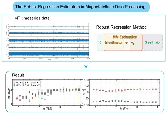
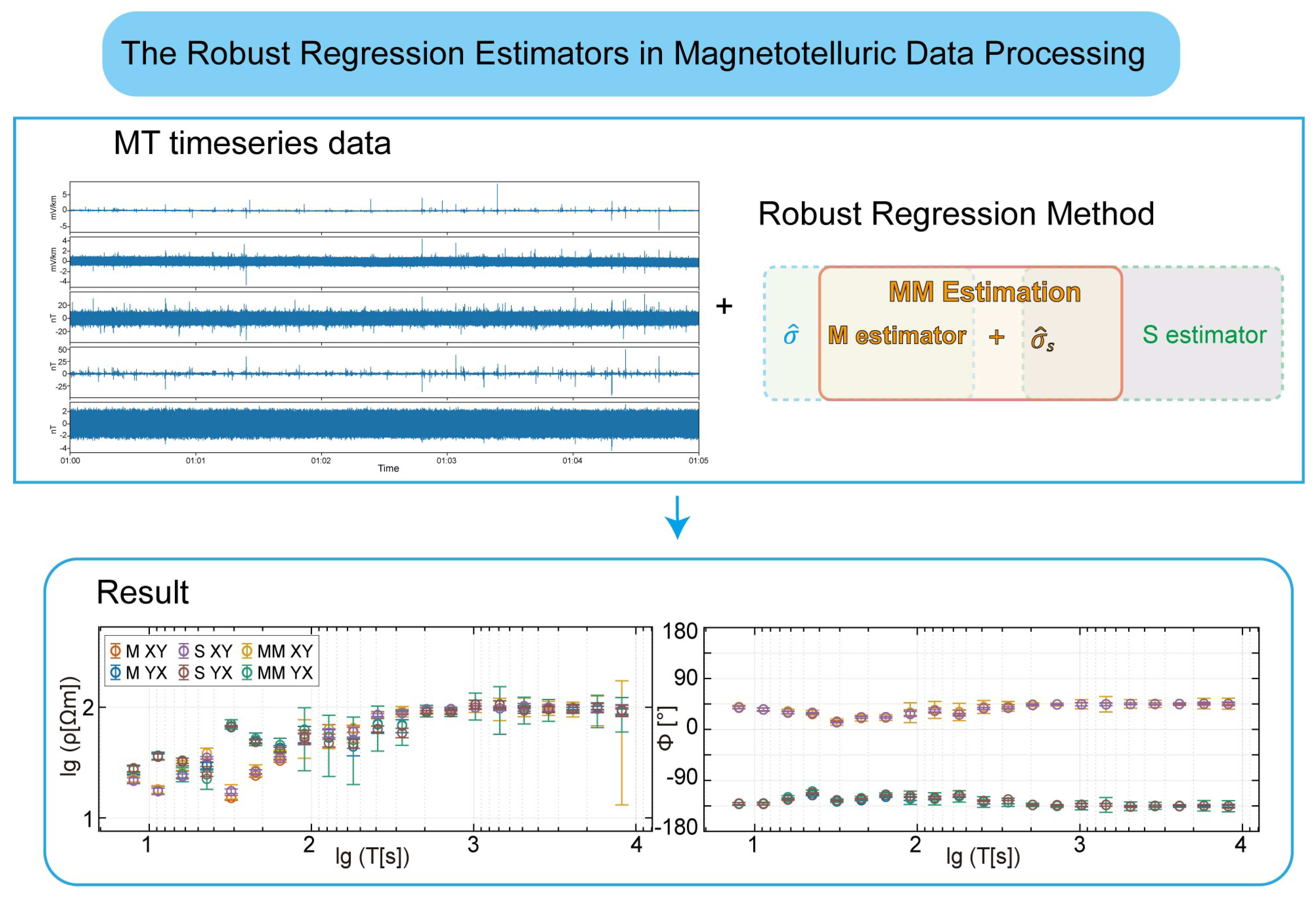
Magnetotelluric (MT) transfer functions are commonly estimated using statistical regression methods. Reliable MT-derived geoelectrical structures are essential for investigating deep geodynamic processes and metallogenic systems; however, noise contamination can distort impedance estimates and lead to misleading geological interpretations. In this study, we introduced an MM-estimator into MT data processing and evaluated its performance alongside M- and S-estimators using synthetic examples and an MT data survey from northeastern China. The results indicate that all three estimation methods can effectively suppress complex background noise and improve the stability and reliability of MT impedance estimation. The methods produced generally consistent apparent resistivity and phase responses, with MM-estimator yielding relatively the lowest root-mean-square (RMS) values. However, the deviations–uncertainty trade-off should be carefully evaluated in practical applications, particularly when processing long-period MT data with MM-estimator. Finally, we suggest combining any of the three robust estimation methods with the remote reference technique to help suppress noise in both predictor variables (magnetic-field data) and dependent variables (electric-field data).

Graphical Abstract

1. Introduction

As a conventional electromagnetic (EM) geophysical method, the magnetotelluric (MT) method is widely used to investigate subsurface geoelectrical structures, including crustal and/or lithospheric architecture, deep geodynamic processes, resource exploration, and orogenic deformation systems. In particular, subsurface electrical structures provide important constraints on metallogenic systems, as conductive anomalies are commonly associated with magma reservoirs, fluid migration pathways, partial melts, and fault-controlled weak zones, all of which play critical roles in mineral-deposit-forming processes. Numerous classical MT studies have demonstrated the ability of electrical resistivity models to reveal subsurface structures related to mineralization [1,2,3,4,5,6]. Among these, Heinson et al. [3,4] presented a detailed resistivity model from the Olympic Dam district in Australia, demonstrating that MT-derived electrical structures can provide valuable insights into geological settings associated with mineral deposits. However, acquiring high-quality EM field data in mining areas is generally challenging, as they are usually dominated by complex cultural EM noise. Such noise can distort MT transfer functions, introduce uncertainties into impedance estimation, and potentially degrade the quality of subsequent inversion results. Therefore, improving the robustness of MT impedance estimation is an important step toward obtaining reliable resistivity models and supporting future geological interpretation.
MT transfer functions are derived from orthogonal, naturally varying EM fields. Individual estimates of the transfer functions and cross-power spectral density matrices are computed from discrete Fourier spectra obtained via short-time Fourier transforms applied to individual time windows. Under noise-free conditions, the frequency-dependent impedance tensor Z ( ω ) is defined as [7,8,9]:
E x ω E y ω = Z x x ω Z x y ω Z y x ω Z y y ω H x ω H y ω ,
where H x and H y denote the magnetic-field components and E x and E y denote the electric-field components. In practice, EM signals are generally contaminated with background noise, and the linear regression system is typically expressed as:
r = E Z H
where r = ( r x , r y ) is the residual of the dependent variable (i.e., E = ( E x , E y ) ) for each time window at a frequency of ω . The ordinary least-squares (LS) method minimizes the Euclidean norm of the residuals and is therefore sensitive to outliers when the Gaussian noise assumption is violated. Since the early development of MT, various statistical approaches have been proposed for robust impedance estimation [10,11,12,13,14,15,16,17].
On the other hand, outliers associated with predictor variables, i.e., magnetic-field data, are commonly referred to as leverage points [18,19]. Since conventional residual-based robust estimators mainly reduce the influence of observations with large residuals, they may still be affected by high-leverage observations in the predictor space. The remote reference technique was proposed to suppress local magnetic noise that is uncorrelated with the noise at reference stations [20,21,22]. When a remote reference station is available, both robust estimation methods and remote reference technique are typically employed in combination [12,15,23,24]. However, if both local and reference channels are contaminated by correlated noise, the results from the remote reference method will be distorted [25,26].
Unlike the classical remote reference approach, which incorporates the cross-power spectral density between the local and reference magnetic fields into the spectral density matrix, other algorithms have been proposed to suppress leverage points associated with noise in the local magnetic field. The two-stage bounded influence estimator is one of the effective methods for removing correlated noise in local EM fields using clean remote stations [18,27]. Since the remote reference technique can be considered a two-input–multiple-output linear system, Usui et al. [17] proposed a robust remote reference estimator based on robust multivariate linear regression. Ogawa et al. [28] separated signals from noise-affected components by applying frequency-domain independent component analysis to both local EM data and reference magnetic data. A similar approach based on frequency-domain independent component analysis was proposed by Sato et al. [29]. It is worth noting that high-quality reference data are generally required by both conventional and derivative remote reference methods. Furthermore, when array MT stations and synchronous data are available, a robust multivariate errors-in-variables estimator that utilizes principal component analysis has proven to be a practical approach for extracting signals corresponding to the two polarizations of plane-wave MT fields [30,31,32]. Smirnov and Egbert [33] further extended the multiple-station technique [31] for application to large incomplete arrays, accommodating practical deployment strategies such as the “rolling array”.
Pre-screening of data segments in the frequency domain is generally employed prior to robust estimation methods and/or remote reference technique to exclude severely noisy data. Various pre-selection strategies have been proposed in previous studies, and we outline some of these strategies below. To address low signal-to-noise ratios in the dead band, Egbert and Livelybrooks [14] selected only data segments with high electric-to-magnetic-field multiple coherence. Signals with a magnitude significantly higher than the self-noise (sensitivity) of magnetic sensors were selected as effective data [34]. In auroral zones, limited vertical magnetic-field variations were considered indicative of data contaminated by non-uniform sources [35]. In a more general context, two partial coherences calculated from orthogonal electric-field and magnetic-field components were suggested as criteria for removing highly noisy segments [16]. Moreover, physical properties, including spectral power densities, polarization directions, and coherences, were evaluated to improve MT transfer functions [36], and a further automated pre-selection approach based on Mahalanobis distance and magnetic-field constraints was developed by Platz and Weckmann [37]. A multi-criteria data sorting strategy was suggested by Wang et al. [38].
In addition, various time-domain approaches have been employed to enhance data quality, including time-series denoising using mathematical transforms [39,40], decomposition methods [41,42], digital signal filtering [43], autoregressive models [16], and signal reconstruction algorithms based on compressive sensing [44], among many others not listed here. It should be acknowledged that artificial neural networks offer distinct advantages in time-series data cleaning [45,46]. Conventional artificial neural networks have been applied to MT data processing and perform well for typical synthetic noise [47,48,49,50,51,52]; however, misfits are inevitable when the data contain complex, persistent, or long-duration noise. Furthermore, supervised-learning-based approaches typically require time-consuming manual identification and labeling [45], and the robustness of the trained models depends on relatively large datasets, which can be challenging to obtain. Unsupervised-learning-based approaches typically require careful parameter selection to achieve optimal performance [53,54,55], which remains challenging in practical applications.
Although various approaches in both the time and frequency domains are generally employed to obtain final transfer functions, robust techniques combined with the remote reference method remain the most practical and widely adopted approaches for addressing the frequency-dependent linear regression relationships between orthogonal EM fields. In practice, the most widely used approach is M-estimator [56], which generalizes the maximum-likelihood framework. M-estimator employs the median absolute deviation as a univariate scale estimator, which is independent of the overall data distribution [57]. An alternative approach is S-estimator [58], which is based on robust scale estimators. Usui et al. [17] applied S-estimator to their multiple-output system and illustrated the differences between M- and S-estimators using a simple linear regression problem. To combine the high robustness and high breakdown point of S-estimator and the efficiency of M-estimator, MM-estimator was subsequently proposed by Yohai [59]. Theoretically, the performance of different estimators is expected to vary across typical statistical scenarios.
It is difficult to evaluate the contribution of time- and/or frequency-dependent algorithms to noise suppression from time-series data to transfer functions because of complex and varying EM noise. Although a combination of all possible approaches in both the time and frequency domains seems to be an optimal strategy, it is still meaningful to analyze the performance of a specific method. In this study, we developed a robust estimation method based on MM-estimator and applied M-, S-, and MM-estimators to both synthetic and field MT datasets to evaluate their performance. Our study suggests that a comprehensive comparative analysis of results obtained from different estimation methods combined with remote reference techniques should be conducted in practical applications, thereby enhancing studies on mineralization mechanisms.

2. Theory and Methods

2.1. MT Data Processing

Here, we briefly describe the basic procedures of MT data processing, while detailed descriptions can be found in previous studies [16,17,27,60]. Time-series data of observed orthogonal EM fields are generally checked and/or corrected using time-domain approaches, including filtering, artificial neural networks, decomposition methods, and others. Pre-cleaned time-series data are then subdivided into overlapping data segments (time windows), followed by cascaded decimation with low-pass filtering. In general, analysis and processing proceed for each data segment as follows: (1) Pre-whitening is performed to remove long-period trends and mean values. (2) The segment is tapered using a Hanning or Hamming window to reduce spectral leakage. (3) Fast Fourier transforms (FFTs) are performed to obtain Fourier coefficients for all channels, and calibration correction is also applied. (4) A spectral density matrix consisting of auto- and cross-spectral densities is calculated. (5) Frequency-domain pre-selection is carried out using coherence sorting and other methods.
As a result of the above steps, spectral density matrices from all segments at specified evaluation frequencies are prepared for the subsequent regression procedures.

2.2. Robust Estimation Methods

M-estimator provides a robust generalization of the classical LS method (“M” denotes “maximum-likelihood-type”) [56]. For the linear regression problem defined in Equations (1) and (2), M-estimator introduces a general loss function, ρ, and minimizes the following objective function for each regressor corresponding to either r x or r y :
θ ^ M = arg min θ ^ i = 1 N ρ r i θ ^ ,
where θ ^ denotes the estimator, r i denotes the general residual of either r x or r y at a frequency of ω for the i-th segment (time window), and N denotes the total number of observations, i.e., the number of time windows. In general, the same procedures are applied to the observation equations (for either E x ω or E y ω ). The Huber function [56] and Tukey’s bisquare function [61] are commonly employed as the loss function ρ . A scale estimate based on the median absolute deviation is typically used, because it is less sensitive to outliers [57].
In practice, the estimating equation based on standardized residuals is given by Equation (4) [62]:
i = 1 N ψ r i σ ^ H i = 0 ,
where ψ is the derivative of ρ . σ ^ is a scale parameter:
σ ^ = M A D 0.6745 = m e d i a n r i m e d i a n r i 0.6745 .
To solve the non-linear optimization problem in Equation (4), the iteratively reweighted least-squares (IRLS) algorithm is typically used. The core idea is to transform the objective function of robust estimator into a weighted least-squares problem, where the weights depend on residuals from the previous iteration. Specifically, the weight matrix at the k -th iteration is defined as W ( k ) = d i a g w ( r 1 k ) , , w ( r n k ) , where w (⋅) is a weight function of standardized residuals:
i = 1 N w r i ( k ) σ ^ ( k ) H i = 0 .
Consequently, the updated estimator in Equation (6) can be explicitly formulated as follows:
Z ^ k + 1 = H H W k H 1 H H W k E .
Although conventional M-estimator provides robustness against vertical outliers in the response variables, it remains sensitive to high-leverage observations in the predictor matrix. In MT impedance estimation, leverage points may originate from contaminated magnetic-field spectra or contaminated predictor channels, which can significantly influence the regression solution. Therefore, a leverage-adjusted weighting scheme was adopted in this study.
The final weight assigned to each observation is defined as:
w i = w u i w h i ,
where w ( u i ) represents the residual-based robust weight obtained from the standardized residual u i = r i σ ^ and w ( h i ) is the leverage weight used to reduce the influence of high-leverage observations. The leverage value h i is calculated from the diagonal elements of the hat matrix:
h i = H H H H 1 H H i i ,
where h i measures the relative contribution of the i-th observation to the fitted regression model.
In this study, we employed Tukey’s bisquare weight function (Equation (10)) [61] as the weighting scheme in the estimation procedure:
w u i = 1 u i c 2 2 , u i c 0 , u i > c ,
Under the assumption of a normal distribution, the estimator achieves approximately 95% asymptotic efficiency when c = 4.685 . The leverage weights w ( h i ) are obtained using Tukey’s bisquare function applied to the normalized leverage values.
To overcome the limitations of the median-based scale in M-estimator, S-estimator employs the residual standard deviation [57] and is formulated to minimize the scale of the residuals as shown in Equation (11) [62]:
θ ^ s = arg min θ ^ σ ^ s r 1 θ ^ , , r N θ ^ ,
where σ ^ s is obtained by solving Equation (12):
1 N i = 1 N ρ r i σ ^ s = K ,
where K represents the expected value of the chosen loss function ρ under the standard normal distribution. For high-breakdown-point S-estimator, a commonly used value is K 0.199 . The initial estimate of σ ^ s is obtained from Equation (5), and the iterative update equation is given as follows:
σ ^ s k + 1 = σ ^ s k 1 N K i = 1 N ρ r i σ ^ s k .
S-estimator [58] incorporates a robust scale estimator and attenuates the influence of outliers by minimizing a scale-based criterion for the residuals. Due to the non-convex nature of the S-estimator objective function, a multi-start strategy is employed, where each independent run is initialized from a random subset. In this study, 10 random starting points were used to improve the reliability of the solution, and the final solution was selected as the one yielding the minimum scale.
One key distinction between S-estimator and M-estimator is that S-estimator minimizes its objective function by iteratively updating the scale parameter σ ^ s until no further decrease in the residual scale is observed. Accordingly, Equation (4) can be reformulated into the form given in Equation (14):
i = 1 N ψ r i σ ^ s H i = 0 .
M-estimator provides good robustness against vertical outliers by reducing the contribution of observations with large residuals through the IRLS procedure. In contrast, S-estimator achieves a high breakdown point through constrained scale estimation; however, this robustness comes at the cost of increased computational complexity. Similar to M-estimator, leverage weights are additionally incorporated into the S-estimator procedure in this study to further suppress the influence of high-leverage observations. Consequently, S-estimator is typically used as the initial stage of MM-estimator, while the subsequent refinement is carried out using M-estimator [59].
Specifically, MM-estimator begins by computing a high-breakdown scale parameter σ ^ s by solving Equation (12) using S-estimator. Based on this initial scale estimate, an M-estimator is subsequently performed using the weight function in Equation (10), thereby achieving high statistical efficiency. In addition, leverage weights derived from the hat matrix are incorporated into the weighting scheme to reduce the influence of high-leverage observations. The final MM-estimator is then obtained by solving the following estimating equation:
i = 1 N ψ r i σ ^ M M H i = 0 .
In practice, the three approaches are typically implemented using an iterative strategy, in which specific scale definitions and estimating functions are applied for M- and S-estimators, while MM-estimator performs M-estimator using the robust scale obtained from S-estimator. For all three estimation methods, the IRLS procedure was terminated when the relative change in the residuals between two consecutive iterations became smaller than the predefined tolerance tol, which was set to 10 4 in this study:
r ( k + 1 ) r ( k ) 2 r ( k + 1 ) 2 < t o l ,
or when the maximum number of iterations (100 in this study) was reached.
Figure 1 illustrates the algorithmic workflows of the three robust estimation methods. The detailed procedures are described as follows:
  • Initialization: The impedance tensor Z ( 0 ) is initialized using the ordinary least-squares (OLS) method.
  • Residual computation: For the current estimate Z ( k ) , the residuals r ( k ) are calculated from the observed magnetic-field (H) and electric-field (E) components for all segments (time windows).
  • Scale estimator and residual updating:
    • M-estimator: Compute the scale parameter σ ^ using the median absolute deviation (MAD) and update r ( k ) using M-estimator with σ ^ .
    • S-estimator: Initialize the scale parameter σ ^ s using MAD, then update σ ^ s according to Equation (12). The residuals r ( k ) are updated using S-estimator with the updated σ ^ s . A multi-start strategy with random initial subsets is employed, and the solution with the minimum robust scale is selected.
    • MM-estimator: Update r ( k ) using M-estimator together with the scale parameter σ ^ s obtained from S-estimator.
  • Impedance tensor update: The impedance tensor Z ( k ) is updated based on the weighted residuals r ( k ) .
  • Iteration: Repeat steps 2–4 until the number of iterations reaches the predefined maximum value or the residuals between two consecutive iterations are less than the predefined tolerance value.

3. Implementation

3.1. Synthetic Experiments

3.1.1. Synthetic Data

To ensure that the synthetic experiments are controlled by artificially imposed noise only, we prepared a clean time-series dataset by computing the electric-field response of a theoretical model to observed magnetic-field data. Raw MT time-series data were sampled at 0.5 Hz with a total duration of approximately 10 days using a LEMI-423 instrument. The measured magnetic flux density B ( t ) was first converted into magnetic field intensity H ( t ) using:
B t = μ 0 H t ,
where μ 0 is the magnetic permeability of free space. In the frequency domain, the horizontal electric-field components were computed using the impedance tensor (Equation (1)).
We defined a homogeneous half-space model with a resistivity of 100 Ω·m, for which the impedance is defined as:
Z ω = i ω μ 0 σ ,
where σ is electrical conductivity, i.e., 0.01 S/m.
To mitigate spectral leakage caused by long time series, the data were processed using a segmented windowing approach. Each segment was transformed into the frequency domain via FFT, multiplied by the impedance, and then transformed back using inverse FFT. The final time series were reconstructed using weighted overlap-add, where the weights were derived from the window functions.
The theoretical magnetic fields were then reconstructed from the synthetic electric field. A stabilized inverse formulation was adopted:
H x ω H y ω = 0 Z ω Z ω 0 1 E x ω E y ω .
The vertical magnetic field was obtained using tipper transfer functions:
H z ω = T x ω H x ω + T y ω H y ω .
Both horizontal and vertical magnetic fields were subsequently converted back to magnetic flux density.

3.1.2. Results of Robust Estimation Methods

To evaluate the robustness of the proposed estimation methods, different types of noise, including Gaussian, square, peak, and sawtooth noise, were added to clean synthetic MT time-series data. These four types of noise are generally regarded as typical EM noise encountered in practical MT data observations and have been widely employed in previous denoising studies in both the time and frequency domains [47,48,49,50,51,52]. The amplitude–frequency characteristics of the noise were controlled via the signal-to-noise ratio (SNR):
S N R = 20 l o g 10 σ s i g n a l σ n o i s e .
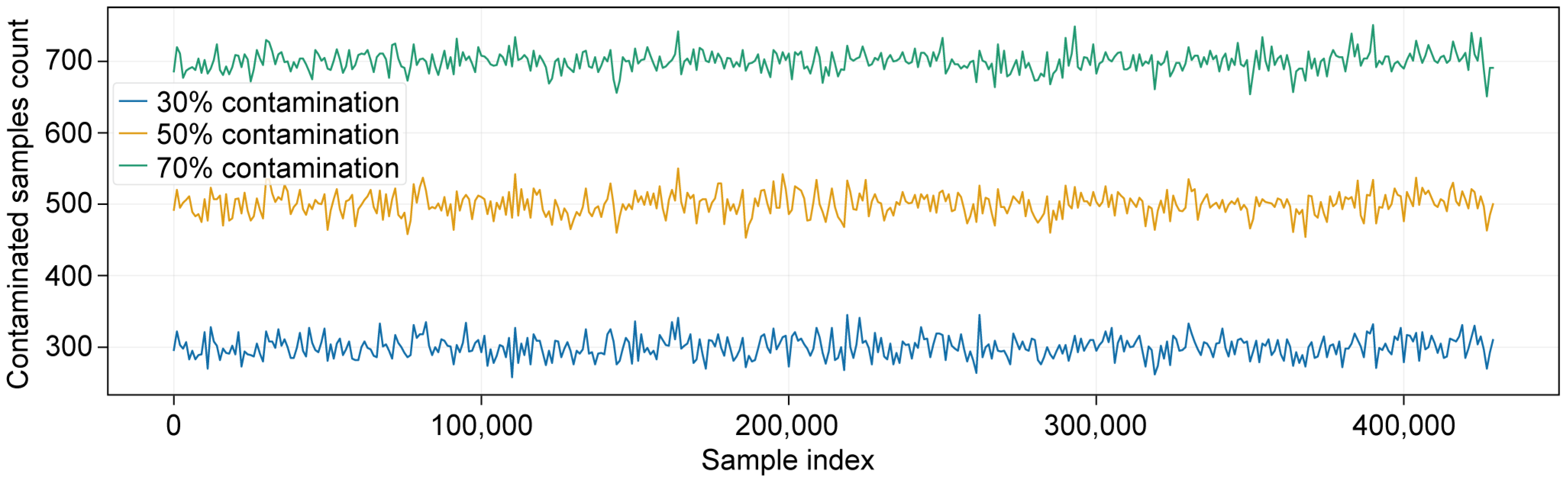
To simulate non-stationary EM contamination patterns, noise was superimposed on randomly selected subsets of samples. Table 1 summarizes the parameter settings for the four types of noise added to the time series. The contaminated data were subsequently normalized using a unified SNR control scheme. Specifically, 30%, 50%, and 70% of samples were randomly selected using a fixed random seed to ensure reproducibility, and noise was added to all channels. This strategy preserved the synchronous occurrence of contamination across different channels and more realistically simulated EM interference in practical environments. Two SNR levels were set to 30 dB and 5 dB, respectively.
The distribution of noise-contaminated data generated using parameter settings in Table 1 is presented in Figure 2. The Gaussian, square, peak, and sawtooth noise components were combined to form a mixed-noise sequence, which was then randomly superimposed onto selected samples according to the predefined contamination ratio. As shown in Figure 2, the contaminated samples were distributed throughout the dataset without an intentionally imposed temporal pattern, allowing the objective evaluation of estimator robustness under mixed-noise conditions.
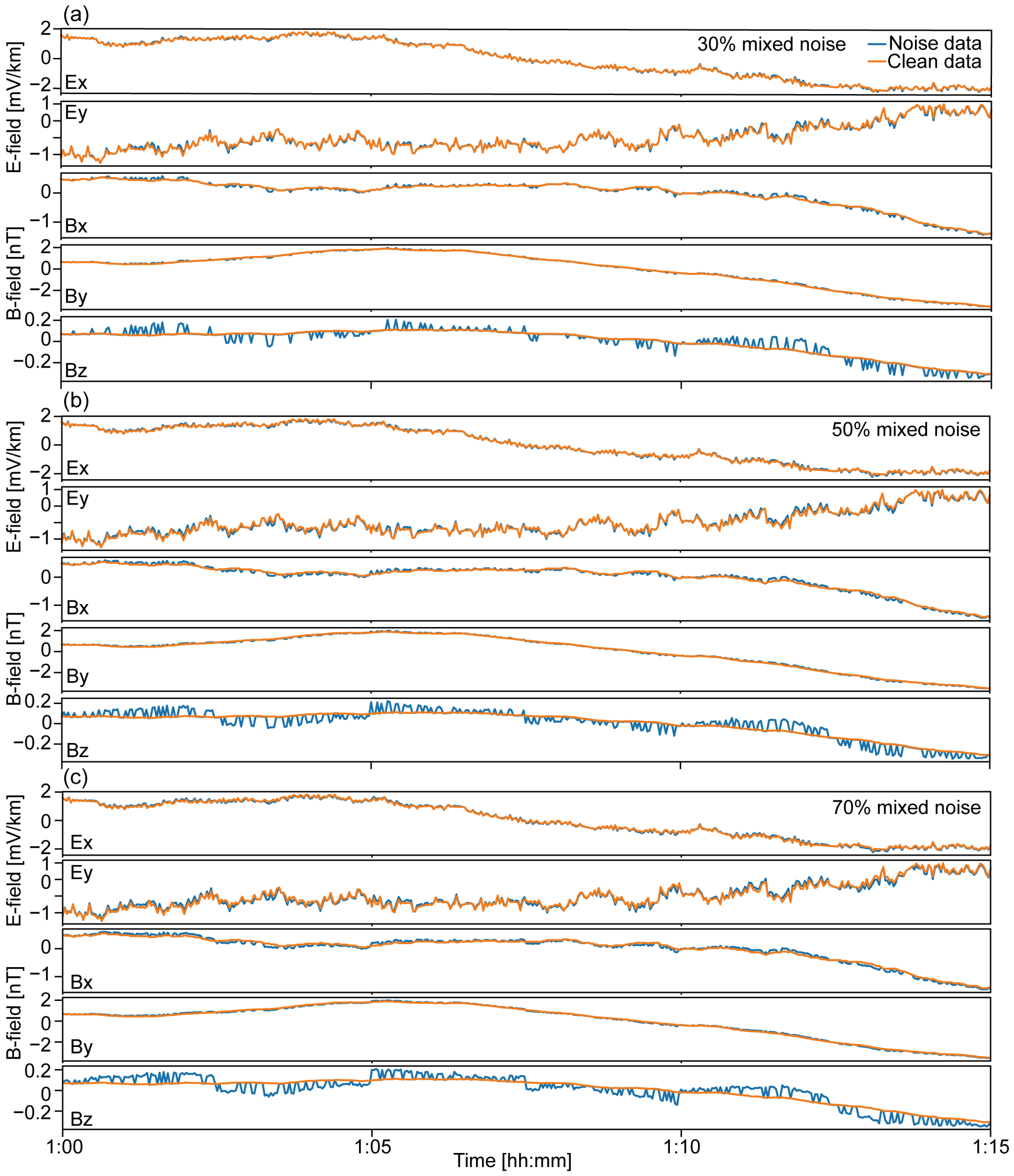
Figure 3 presents comparisons between clean and noise-contaminated time series at an SNR of 30 dB. The standard pre-processing procedures described above were applied to both synthetic and observed datasets in this study. The mean value of each channel was removed to suppress DC components and reduce low-frequency trends. Seven decimation levels were employed, with the sampling frequency reduced by a factor of 8 at each level. Evaluation frequencies were logarithmically distributed at seven frequencies per octave to ensure adequate spectral resolution across the investigated bandwidth. The decimated time series were segmented into overlapping windows of 512 samples with 25% overlap. A Hamming window was applied prior to Fourier transformation to suppress spectral leakage and reduce side-lobe effects. Fourier transforms were performed on each windowed segment to obtain complex spectra for subsequent impedance tensor estimation. Frequency-domain quality control was primarily based on coherence analysis between the electric- and magnetic-field components. No additional frequency selection threshold was applied. Frequency bands without sufficient valid windows were automatically excluded during processing. The available frequency points were determined by the data length and the number of valid windows after decimation. In total, impedance tensors were estimated over frequencies ranging from 1.22 × 10 4 to 0.125 Hz. The numbers of effective windows used for estimation were 1118, 138, and 17 for decimation levels 0, 1, and 2, respectively.
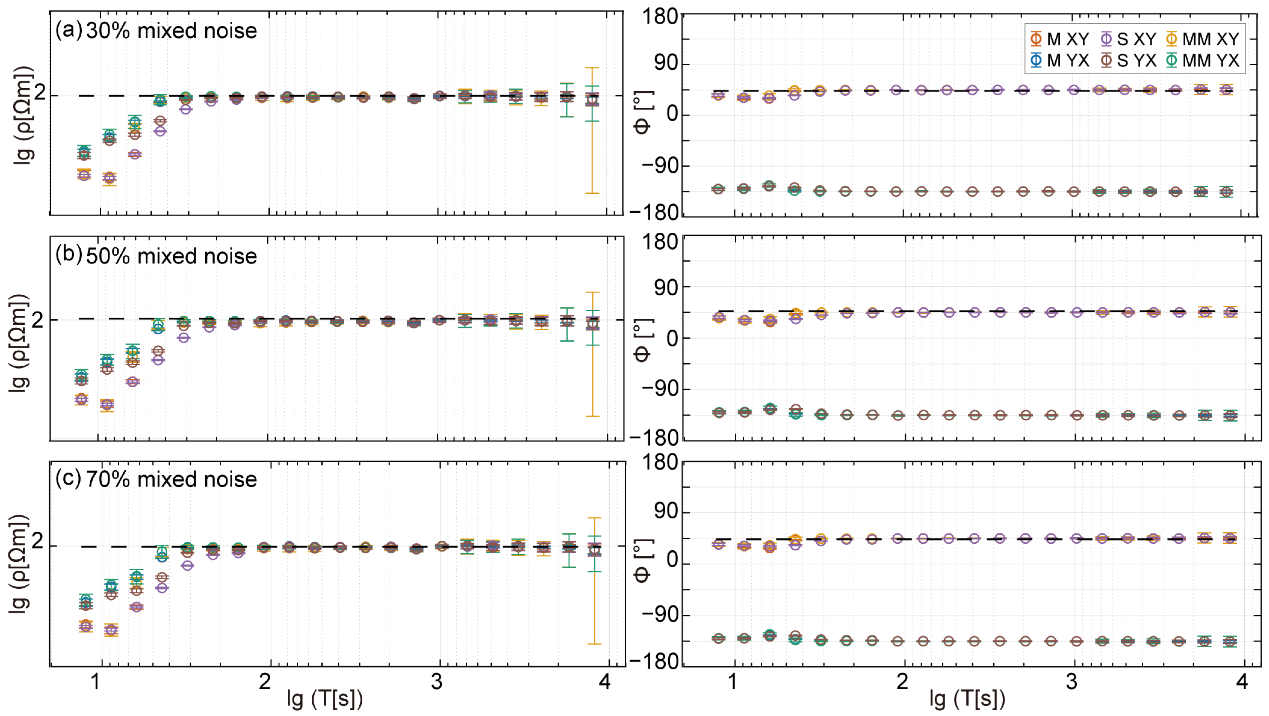
Figure 4 presents the MT sounding results for three synthetic noise contamination scenarios at an SNR of 30 dB, in which Gaussian, square-wave, peak, and sawtooth noise were superimposed on the original clean time series. The contaminated ratios were set to 30%, 50%, and 70%, respectively. The error bars represent propagated 1.96 σ uncertainty estimates of apparent resistivity caused by impedance estimation uncertainty rather than formal confidence intervals based on independent samples. The theoretical response of the homogeneous half-space model, calculated from the analytical impedance solution, is also shown for comparison. All three methods exhibit noticeable deviations from the theoretical apparent resistivity and phase responses at periods shorter than 80 s, indicating that none of the statistical estimators can effectively suppress the complex noise in this short-period range. Overall, as the noise contamination ratio increases from 30% to 70%, the apparent resistivity and phase curves obtained using the three robust estimation methods remain relatively stable and consistent. Only S-estimator exhibits a slight deviation in apparent resistivity at high frequencies, while no obvious distortion is observed in the phase results. These observations indicate that, at an SNR of 30 dB, all three robust estimation methods can effectively suppress the influence of mixed noise except for the short period band.
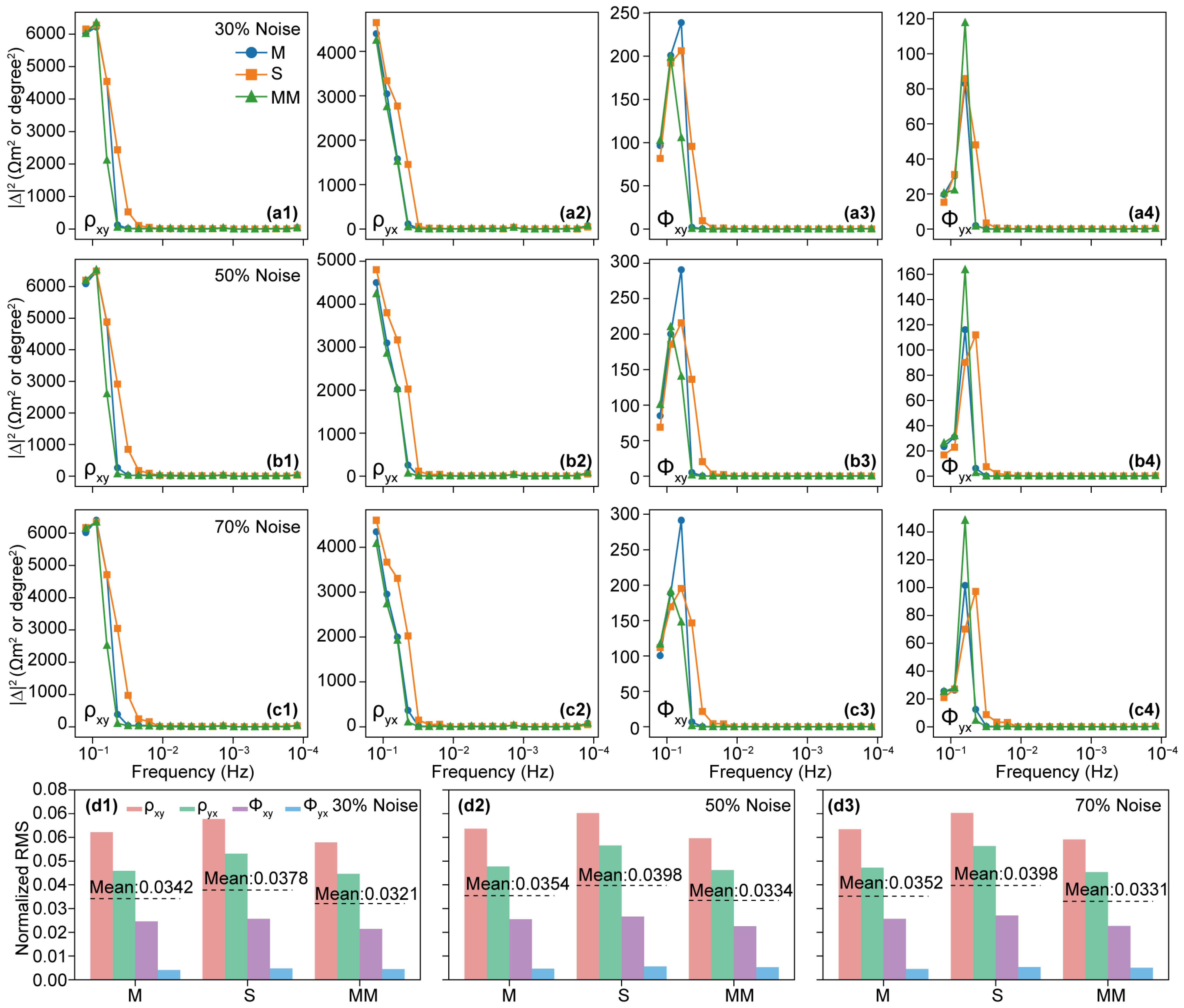
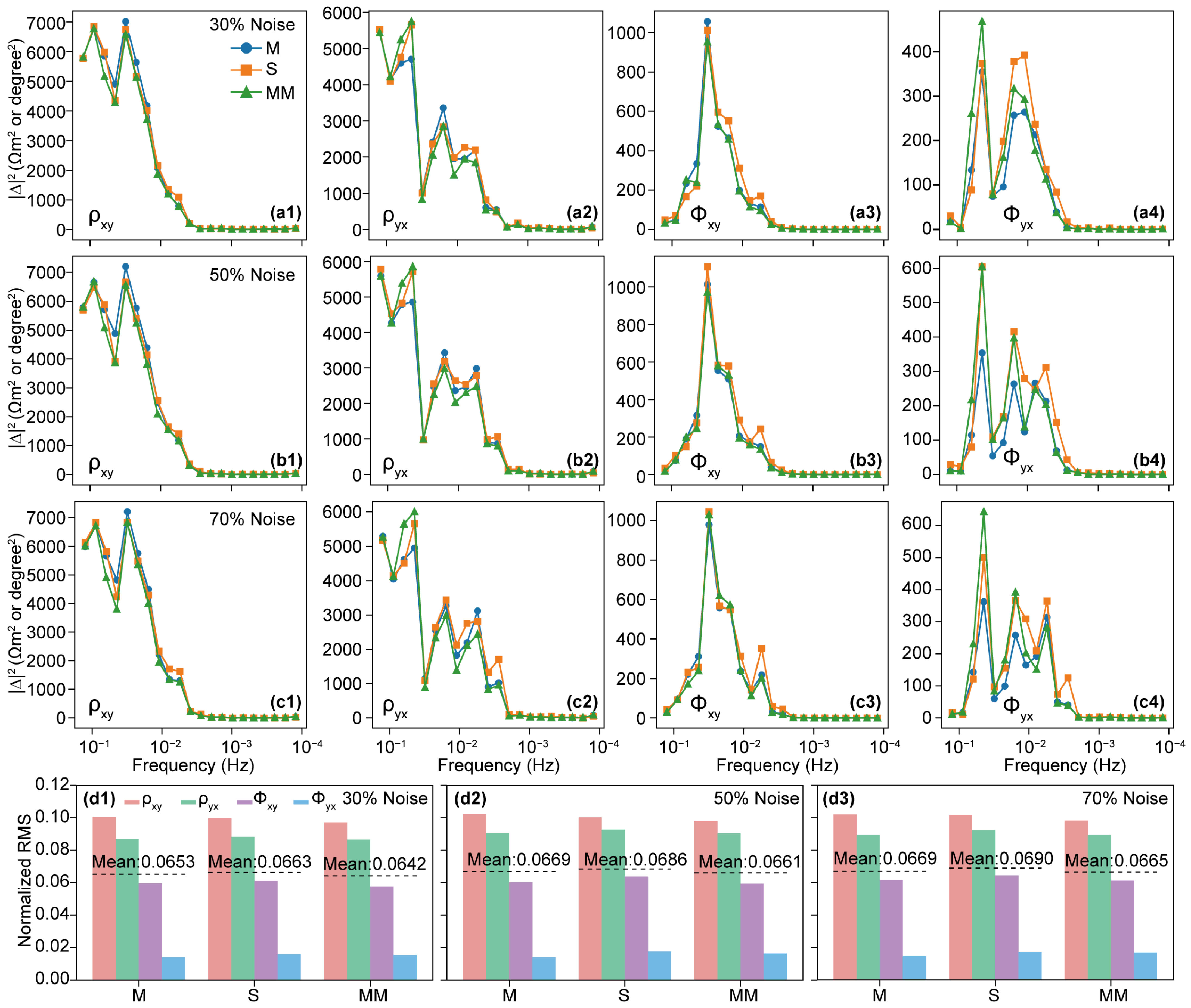
Figure 5 presents the distributions of deviations between the apparent resistivity and phase estimated from noise-contaminated data and the theoretical values. In addition, we calculated normalized root-mean-square (RMS) values for each method. At an SNR of 30 dB, the three methods showed generally consistent deviations, except at high frequencies. The RMS values are highest for S-estimator and lowest for MM-estimator. It is noteworthy that, although the noise contamination ratio increases continuously from 30% to 70%, the phase curves do not exhibit severe distortion or large-scale distortion. The results indicate that all three robust estimation algorithms can effectively down-weight anomalous spectral windows and non-stationary noise segments under low-noise conditions, thereby suppressing the influence of transient interference and intermittent noise on impedance tensor estimation. It is worth noting that, despite MM-estimator yielding a lower RMS error in this experiment, the uncertainties for the long-period data are noticeably increased.
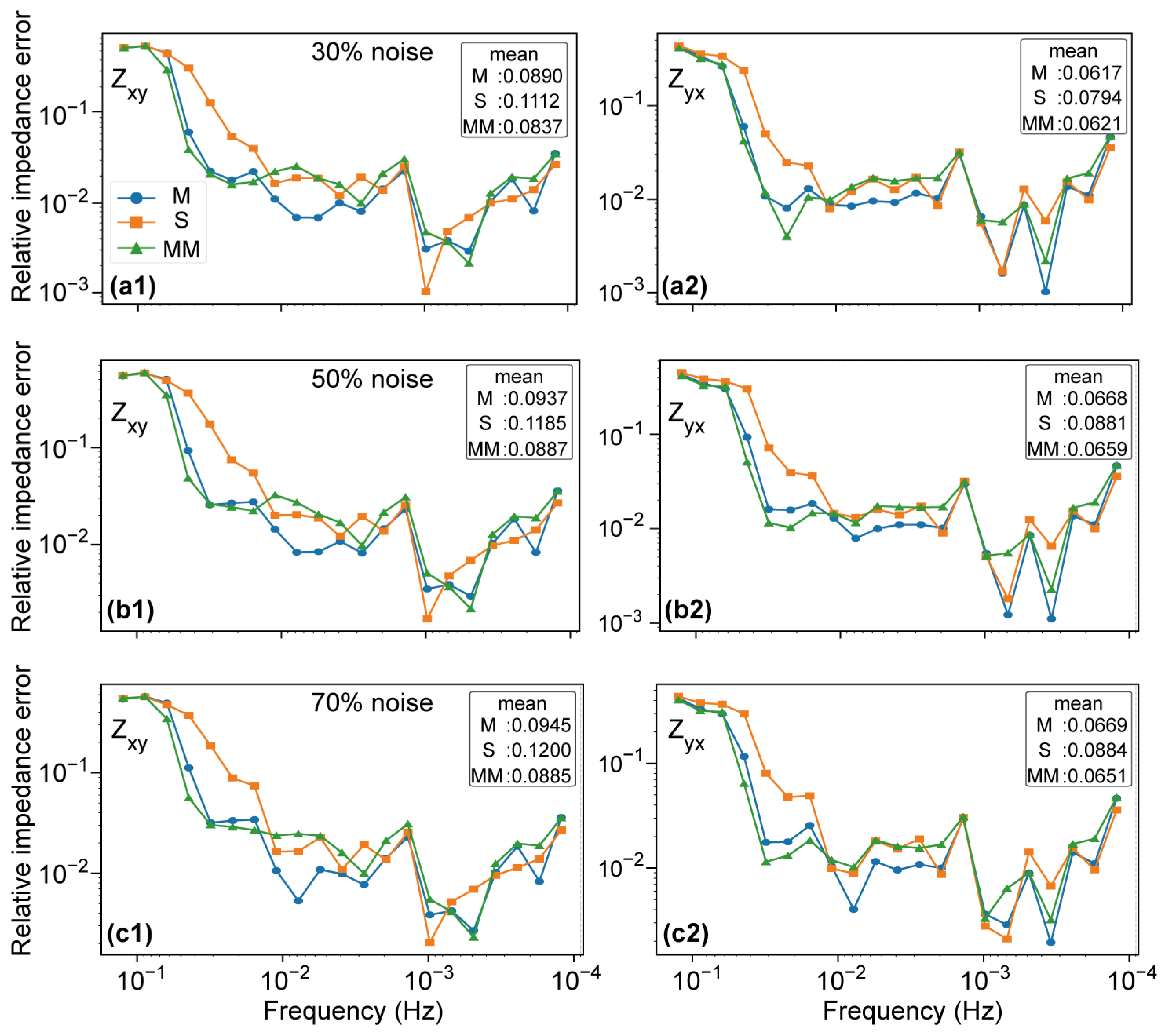
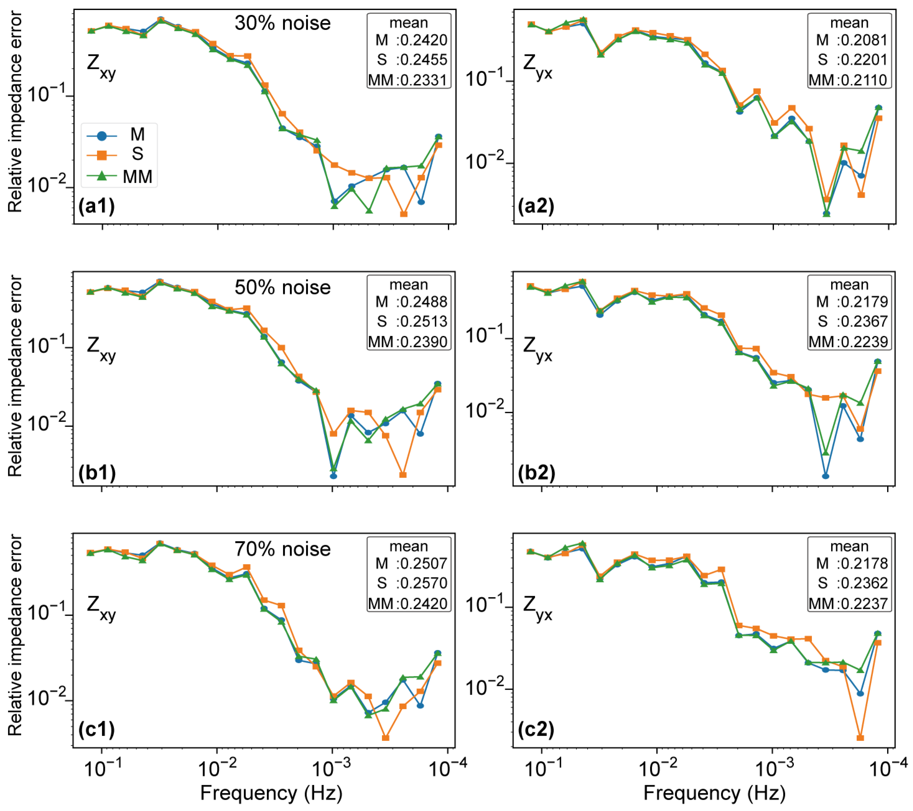
Figure 6 presents the relative complex impedance errors of Z x y and Z y x with respect to the theoretical half-space impedance under an SNR of 30 dB. Under the high-SNR condition, all three estimators achieved low impedance errors, indicating reliable recovery of the theoretical response. Specifically, MM-estimator provided lower or comparable impedance errors in this experiment, particularly for the Z x y component, while M- and S-estimators showed slightly larger variations at some frequencies. The frequency-dependent fluctuations observed in the relative impedance errors are mainly related to the uncertainty of spectral estimation and the varying sensitivity of different impedance components to noise perturbations.
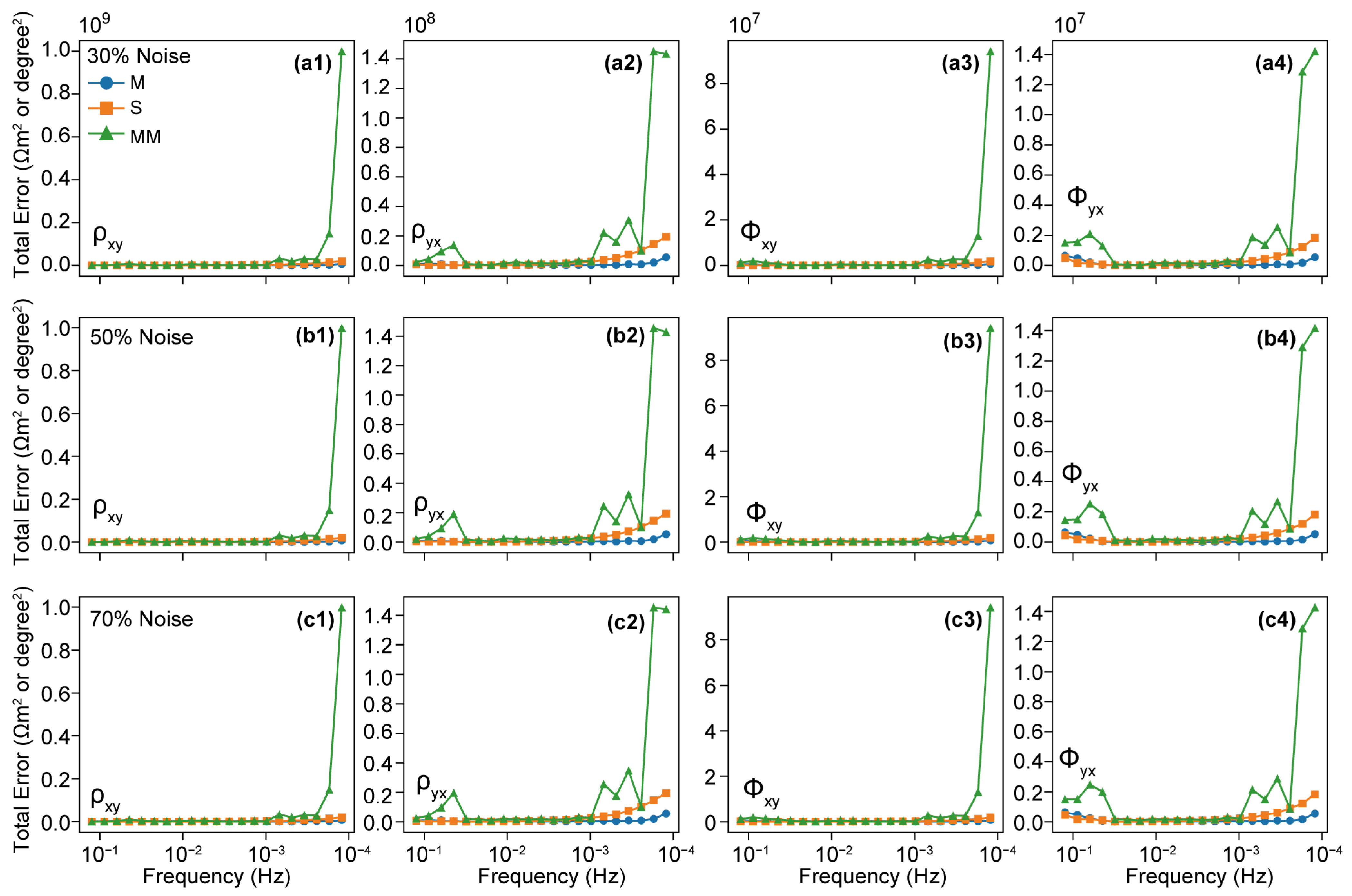
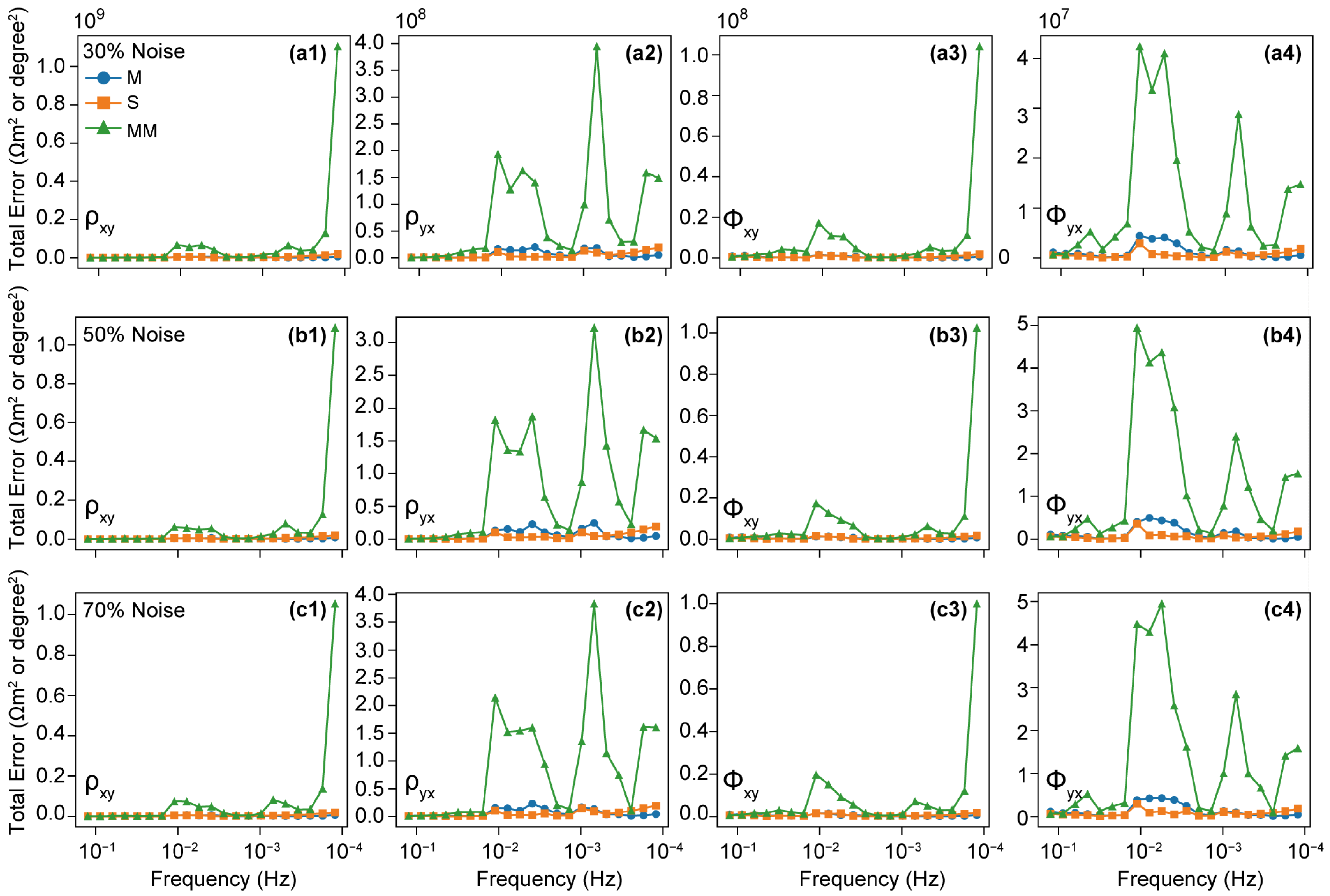
To better understand the comprehensive errors from both RMS deviations and propagated uncertainties, we computed the mean-square error as a Total Error (Total Error = deviations2 + uncertainty), with results shown in Figure 7 for SNR = 30 dB. MM-estimator yielded a notably high Total Error at the longest period, primarily due to increased uncertainty in the long-period range. These results highlight that the deviations–uncertainty trade-off is particularly relevant for long-period MT data and should be taken into account when MM-estimator is applied.
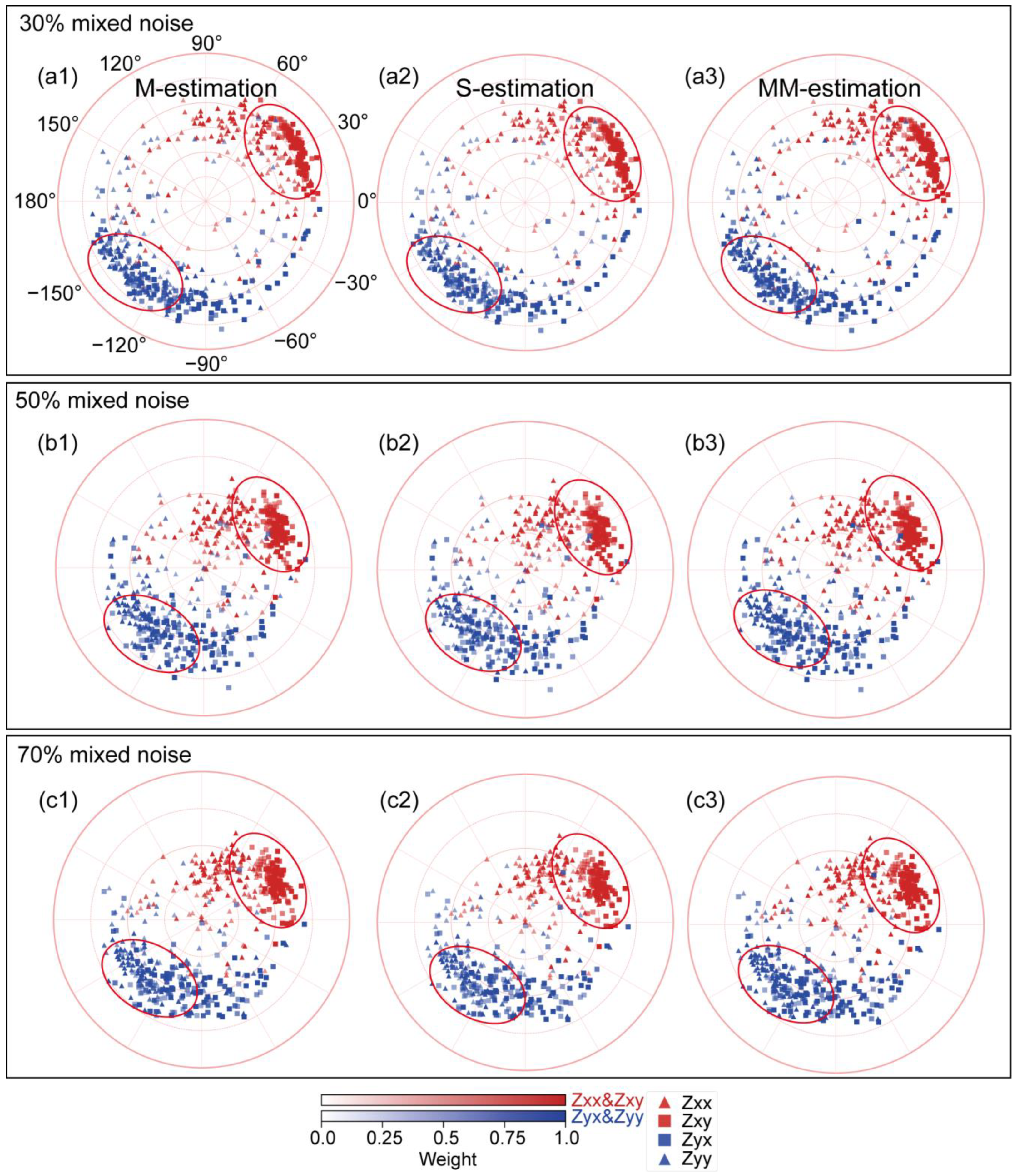
Figure 8 presents the final weight distributions of the impedance tensors at approximately 181 s obtained using different robust estimation methods. The weights were computed from the linear regression models in Equations (1) and (2) and were iteratively updated during the optimization process of each robust estimator. For the Z x y and Z y x components, a common feature across all three cases was that, even as the mixed-noise-contamination ratio increases, all three methods maintained most high-weight points clustered within relatively stable magnitude and phase regions. Together with apparent resistivity and phase results (Figure 4), these weight distributions suggest that the three estimators exhibit robustness and noise resistance under high mixed-noise-contamination conditions.
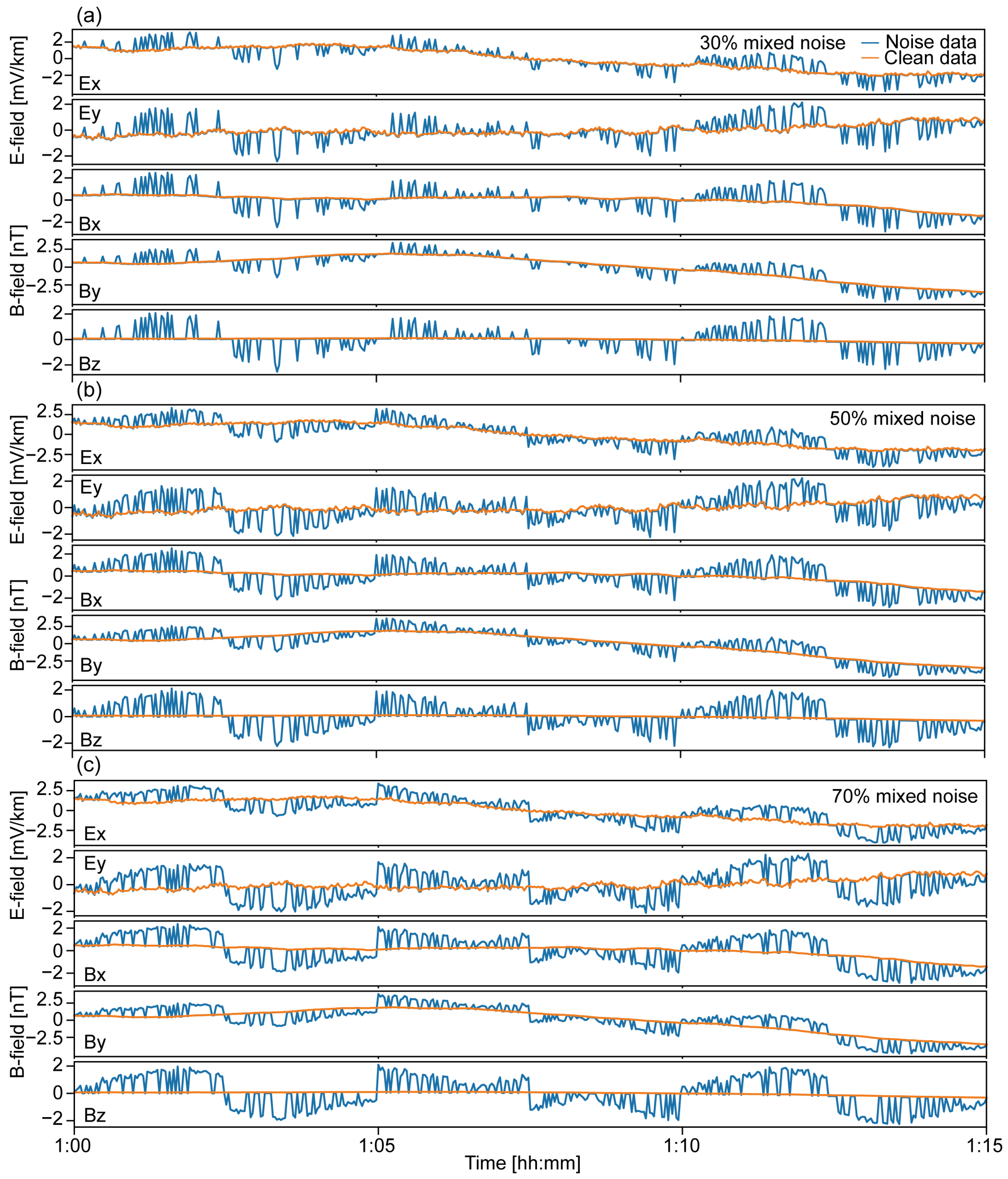
To compare the robustness of the three methods more clearly, the noise intensity was further increased by setting the SNR to 5 dB, while all other conditions remained unchanged. Figure 9 presents a comparison between clean and noise-contaminated time series at an SNR of 5 dB.
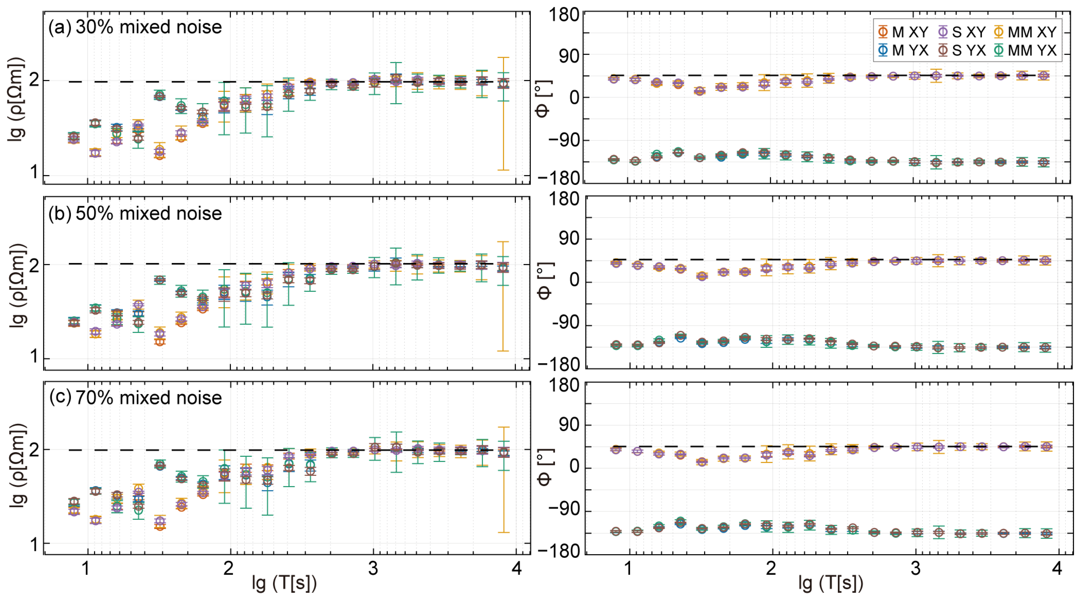
Figure 10 presents the MT sounding results at an SNR of 5 dB for different levels of mixed-noise contamination. The theoretical response of the homogeneous half-space model is included as a reference for evaluating the deviations of impedance estimates under strong-noise conditions. Compared with the results at SNR = 30 dB, the apparent resistivity curves at SNR = 5 dB exhibited greater fluctuations and scattered points for all three robust estimation methods, particularly in the high-frequency range. Additionally, the RMS values were comparable among M-, S-, and MM-estimation methods (Figure 11). These results indicate that, as the background noise level increases, the influence of mixed noise on impedance estimation becomes more pronounced. Nevertheless, despite the intensified noise contamination, all three methods still preserve the overall structural characteristics of the apparent resistivity and phase curves, indicating that the robust estimation procedures reduced the influence of anomalous observations under strong-noise conditions. It is noteworthy that, when the contamination ratio increases from 30% to 70%, the short-period apparent resistivity responses are more strongly affected than the mid- and long-period responses. This is likely because short-period responses are more sensitive to high-frequency transient noise, while the peak and square-wave components of the mixed noise introduce stronger interference in local spectral estimation.
Figure 12 presents the relative complex impedance errors of Z x y and Z y x with respect to the theoretical half-space impedance at an SNR of 5 dB. Compared with the SNR = 30 dB, all estimators showed increased errors and stronger fluctuations due to the increased noise contamination. These results indicate that, as the noise level increases, the influence of mixed noise on impedance tensor estimation becomes more pronounced. It is noteworthy that the relative errors exhibited stronger fluctuations at some frequency points, which may be attributed to the larger uncertainty in spectral estimation under strong noise interference. The different error levels between Z x y and Z y x are likely related to their different sensitivities to noise perturbations and the characteristics of the corresponding regression processes.
Considering the deviations–uncertainty trade-off, MM-estimator exhibits increased uncertainty at long periods, which translates into a larger Total Error (Figure 13), whereas both M-estimator and S-estimator show a slight increase in the Total Error in the mid-period range. This phenomenon reflects the enhanced sensitivity of impedance estimation under high noise levels, resulting in a moderate increase in both estimation errors and propagation uncertainty. This observation, together with the SNR = 30 dB results, suggests that MM-estimator’s slightly lower RMS errors are accompanied by larger propagated uncertainties. This trade-off should be carefully evaluated in practical applications, particularly when processing long-period MT data.
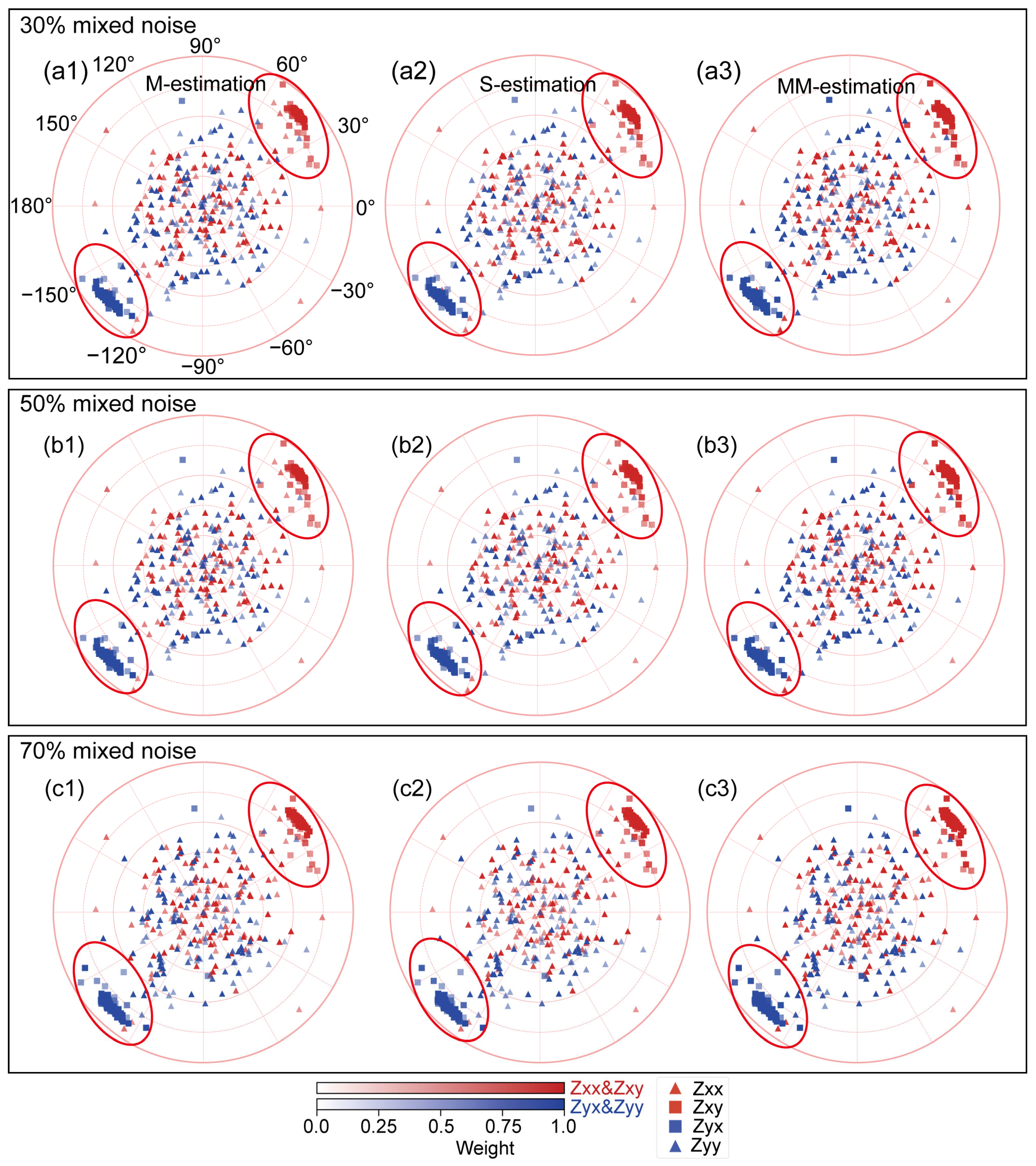
Figure 14 presents the weight distributions of the impedance tensors at approximately 181 s under a noisy condition of SNR = 5 dB. Compared with the results at SNR = 30 dB (Figure 8), the weight distributions in Figure 14 exhibited stronger dispersion, with a noticeable increase in peripheral low-weight points. Nevertheless, all three robust estimation methods still maintain most high-weight points concentrated within relatively stable regions, demonstrating their ability to identify anomalous spectral windows and suppress noise contamination.

3.2. Application to Real Data from Northeastern China

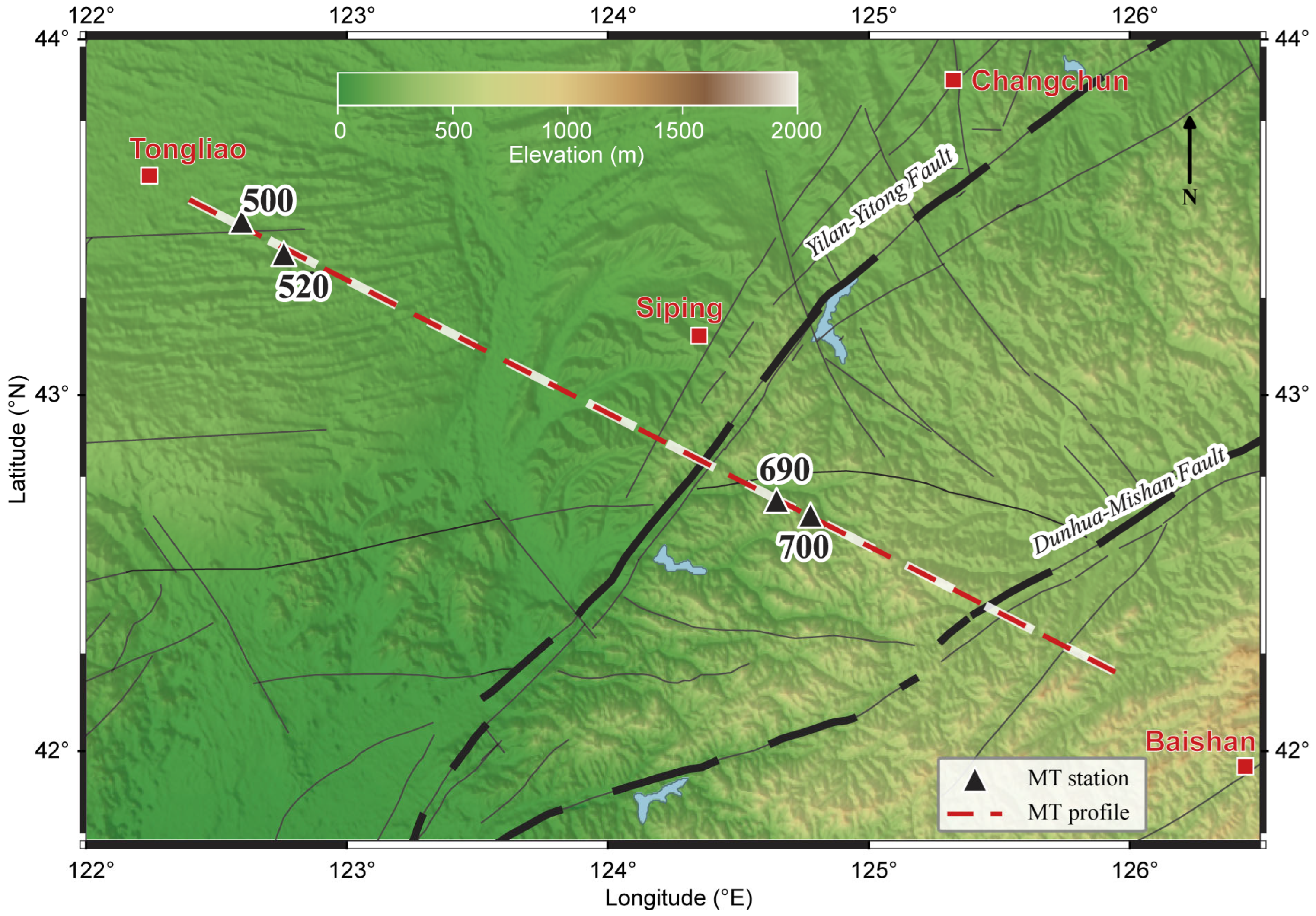
To further evaluate the performance of the robust estimation methods, a remote reference technique was incorporated in the processing of field data. The experimental data are from a northwest–southeast-oriented broadband MT profile deployed in northeastern China [63]. The profile extends from Tongliao, Inner Mongolia, and goes into Baishan, Jilin (Figure 15), an area known for its mineral deposits and oil and gas fields. A total of 32 stations, with an average spacing of 20 km, were occupied in April 2016, using four Metronix ADU-07e instruments. Five orthogonal EM channels were recorded for more than 40 h at each station. The electric fields were measured using EFP06 non-polarizable electrodes, and the magnetic fields were recorded using MFS06 induction coils. The electric dipoles were 100 m for both directions, with E x oriented at 0° (north–south-oriented) and E y oriented at 90° (east–west-oriented). The magnetic sensors were arranged orthogonally, with H x oriented north–south, H y east–west, and H z vertically downward. All magnetic sensors were calibrated before field deployment, and calibration information, including frequency in Hz, magnitude in V/(nT·Hz), and phase in degrees, was recorded.
During the observations, a sampling rate of 4096 Hz was typically used for the first 20 min to capture high-frequency components, after which a sampling rate of 128 Hz was continuously employed for the remainder of the recording period. Stations 520 and 700 served as the local stations, while stations 500 and 690, located approximately 15 km and 12 km away, respectively, were used as remote reference stations. The detailed information of these four stations, including coordinates, elevations, and observation parameters, is summarized in Table 2. A total of 16 h of synchronous data were recorded for stations 520 and 500, while 14 h of synchronous data were recorded for stations 700 and 690. Stations 520 and 700 are separated by approximately 180 km and represent different background geological and noise environments. Our synthetic experiments focused on long-period MT data with a low sampling rate of 0.5 Hz, whereas the field data were recorded at higher sampling rates of 128 Hz and 4096 Hz, indicating that the proposed methods are applicable to both broadband and long-period MT data and can effectively handle multi-scale electromagnetic signals. As in the synthetic experiments, we employed seven decimation levels, reducing the sampling frequency by a factor of 8 at each level. Data windows of 512 samples with 25% overlap were used, and a Hamming window was applied prior to Fourier transformation.
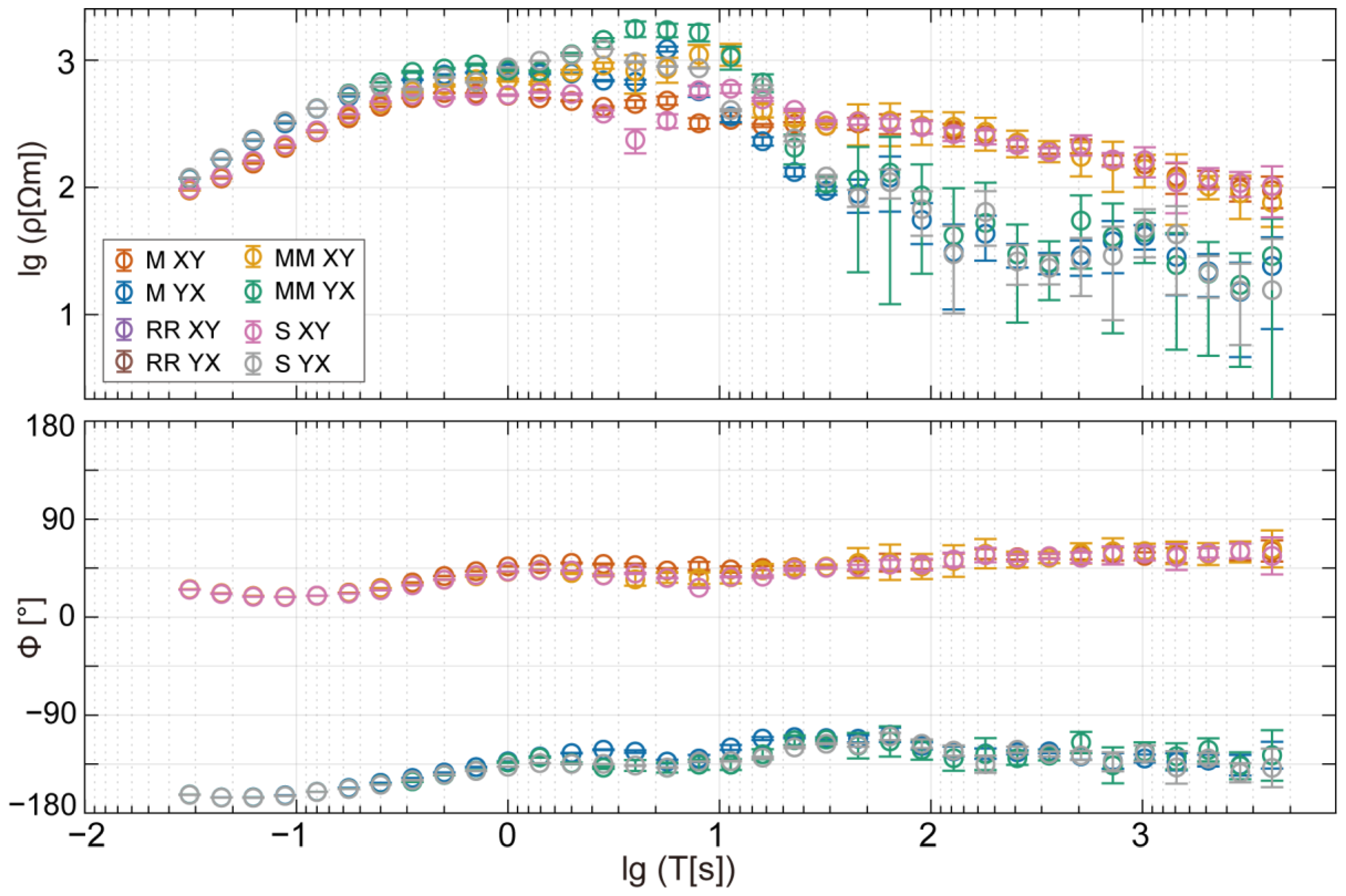
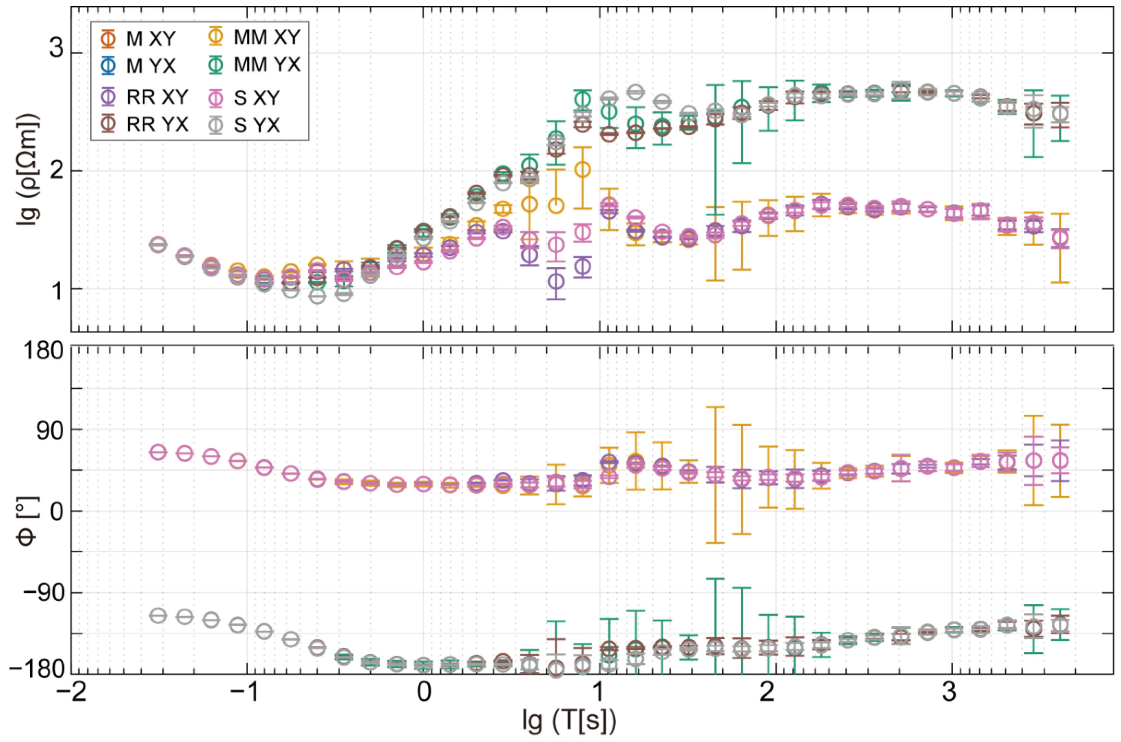
Figure 16 compares the results of station 520 obtained using different methods. Overall, the four methods exhibited consistent trends over most of the investigated period range; however, differences are still observable in the mid- to long-period range. Among the three robust estimation approaches, M-estimator exhibited more noticeable local fluctuations, particularly in the apparent resistivity curves around the intermediate-period range. S-estimator showed relatively smoother transitions and fewer abnormal deviations in the mid- to long-period range. The MM-estimator results again showed larger uncertainties, particularly in the long-period range. Figure 17 shows the results obtained at station 700, where the four estimation methods were in good agreement across most of the investigated period range.
The observed differences among the methods are closely related to their respective robust weighting strategies and statistical properties. These robust estimation methods are primarily based on iterative residual weighting, where the influence of outliers is reduced through a weighting function [64]. It is noteworthy that the remote reference algorithm based on an external reference station may still be preferable in many practical MT scenarios.

4. Discussions

4.1. Theoretical Analysis

Natural EM signals observed in practical MT surveys are often non-stationary, truncated, and contaminated by noise; consequently, the assumption of an ideal normal noise distribution is generally not satisfied for the linear regression model of MT transfer functions (Equations (1) and (2)). The primary distinction among these estimators lies in the definition of their objective functions: M-estimator minimizes a residual-based objective function, whereas S-estimator minimizes a scale-based objective function. These differences lead to different performance characteristics under varying SNR conditions. At SNR = 30 dB, the results obtained using S-estimator exhibited relatively larger fluctuations (Figure 4, Figure 5, Figure 6, Figure 7 and Figure 8). When the SNR decreased to 5 dB, all three methods exhibited larger fluctuations and deviations in the mid- and long-period ranges (Figure 10, Figure 11, Figure 12, Figure 13 and Figure 14). This indicates that the robust estimation methods respond differently to changes in noise intensity, reflecting a clear trade-off between robustness and noise amplitude.
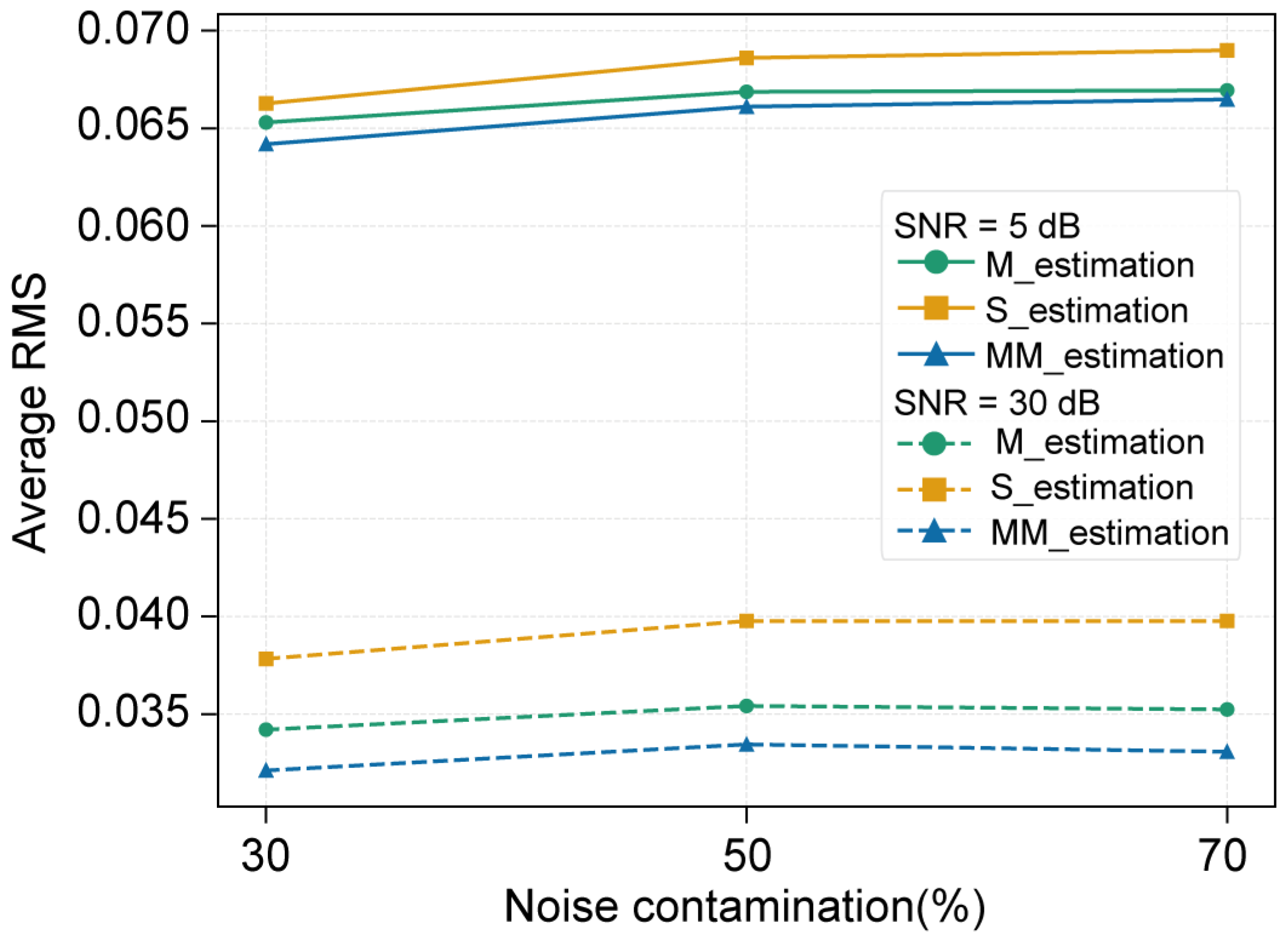
Theoretically, S-estimator employs a high-breakdown-point scale estimation strategy that strongly down-weights spectral windows with large residuals, thereby improving resistance to severe noise contamination. In contrast, the weight adjustment in M-estimator is relatively moderate; however, its ability to suppress outliers remains limited, such that some severely contaminated spectral windows may still retain non-negligible weights. Nevertheless, the results of our synthetic experiments could not provide strong evidence in support of this theoretical analysis. Figure 18 shows the RMS distributions for cases with various noise proportions and SNR levels using different estimators. The results indicate approximately similar RMS values across different noise proportions and methods, with RMS values primarily depending on the SNR. We suggest that both leverage points and SNR play important roles in the estimation process, and even the lower SNR condition of 5 dB used in this study represents non-excessive noise amplitude (Figure 9), such that robustness is largely dominated by SNR for different estimators. A quantitative analysis of the contributions of noise proportion and SNR to the robustness of different estimation approaches would be worthwhile in future studies.
Although a leverage-based weighting strategy using a bisquare function on the hat-matrix diagonal was utilized to limit the influence of high-leverage data points, the three estimators rely on the residuals of the dependent variables (electric-field data). Generally, all orthogonal electric and magnetic channels may be simultaneously contaminated by the local background noise, and we conducted the synthetic experiments primarily based on multi-channel contaminated scenarios. We further calculated the results using data with only electric-field contamination and only magnetic-field contamination (Supplementary Figures S1 and S2). The results indicate that, in the short-period range, the magnetic-field contamination data show obvious distortions compared with the electric-field contamination, suggesting that predictor contamination cannot be fully mitigated, even with leverage weighting. These results suggest that additional methods, such as the remote reference technique or bounded-influence estimators [18,27], are still required to suppress outliers originating from the predictor variables (magnetic-field data). In particular, noise suppression based on additional reference stations remains a practical option when single-station processing is insufficient. Therefore, we further suggest that a combination of each of the three robust estimation methods and the remote reference method could provide advantages in handling both electric-field and magnetic-field noise at local stations.
In addition, Tukey’s bisquare weight function [61] was employed in this study, although the use of alternative weight functions also warrants consideration. Weight functions with bounded ψ-functions can effectively balance robustness and efficiency. During the iterative procedure, the bisquare scheme progressively down-weights outliers, enabling the estimator to focus on the dominant structure of the clean data [65]. Notably, the optimal tuning constants for the weight functions are largely based on classical experience and remain an open issue, calling for adaptive strategies tailored to field datasets with varying noise distributions.

4.2. Limitations and Suggestions

Two major limitations of this study should be acknowledged. First, the synthetic noise scenarios may not fully capture the complexity of cultural EM noise, and natural noise sources—such as long-period geomagnetic variations, instrument drift, and site-specific ground coupling effects—can also produce outliers. Second, the synthetic experiments were conducted by superimposing noise onto randomly selected segments of the time series. This configuration simplifies the noise distributions, ensuring that sufficiently clean windows remain available for robust estimation methods. As a result, the evaluated performance may represent an optimistic estimate of performance compared with real-field conditions. In practical MT surveys, cultural EM interference, instrument grounding issues, and environmental transients are generally persistent, widespread, or intermittently distributed throughout the entire recording. Under such circumstances, the practical robustness of the estimator, the availability of uncontaminated windows, and the convergence behavior of the iterative weighting scheme may all be adversely affected.
In this study, the primary purpose of the synthetic experiments is to evaluate the proposed method. A more comprehensive and quantitative assessment of the estimation approaches would be valuable, particularly by introducing noise scenarios with diverse frequency-domain signatures and a broader range of noise types. Evaluating robust estimators under such realistic and complex noise conditions would help clarify their performance limits and guide the development of adaptive weighting strategies. In addition, further research should focus on integrating adaptive weight selection schemes, multivariate robust estimators, and hybrid approaches that combine frequency-domain robust regression with machine-learning-based time-domain noise suppression.

5. Conclusions

We propose an iterative MM-estimator-based algorithm for the frequency-domain linear regression procedure in MT data processing. Together with the conventional M-estimation and S-estimation methods, we systematically evaluated the performance of all three robust regression estimators using both noise-contaminated synthetic data and field datasets. The results demonstrate that all three estimators can produce reliable impedance tensors when the data are contaminated by a moderate noise level, although the trade-off between robustness and breakdown point under different SNR conditions requires further investigation. Additionally, we conducted experiments using only electric-field-contaminated data and only magnetic-field-contaminated data, respectively, to test the robustness against leverage points, and we suggest combining any of the three estimation methods with the remote reference method to address contamination in the predictor variables (magnetic-field data) and dependent variables (electric-field data) in practice applications.

Supplementary Materials

The following supporting information can be downloaded at: https://www.mdpi.com/article/10.3390/min16080824/s1. Figure S1. Apparent resistivity and phase results estimated using the M-estimation, S-estimation, and MM-estimation methods at an SNR of 5 dB, where 30% of the time-series samples were ran-domly contaminated by mixed noise (noise parameters are listed in Table 1). Panels (a) and (b) show the results obtained when only the electric-field and magnetic-field time series were con-taminated, respectively; Figure S2. Apparent resistivity and phase results estimated using the M-estimation, S-estimation, and MM-estimation methods at an SNR of 5 dB, where 70% of the time-series samples were randomly contaminated by mixed noise (noise parameters are listed in Table 1). Panels (a) and (b) show the results obtained when only the electric-field and magnetic-field time series were contaminated, respectively.

Author Contributions

Conceptualization, W.S. and C.X.; writing—original draft preparation, W.S. and C.X.; writing—review and editing, W.S. and C.X. All authors have read and agreed to the published version of the manuscript.

Funding

This research was funded by the Deep Earth Probe and Mineral Resources Exploration – National Science and Technology Major Project, grant number 2024ZD1000403, and the National Natural Science Foundation of China, grant numbers 42474111 and 42074083.

Data Availability Statement

The datasets generated during the current study are publicly available in the Zenodo repository: https://doi.org/10.5281/zenodo.20197019.

Acknowledgments

We used the high-performance computing facilities at China University of Geosciences (Beijing) for data processing. We thank Tian Jifeng for providing field data for the field-data experiments. Our implementation and code extensions were developed based on the open-source software “resistics” developed by Neeraj Shah. Finally, we would like to thank Stanislaw and anonymous reviewers for their valuable and constructive suggestions and comments on the manuscript.

Conflicts of Interest

The authors declare no conflicts of interest.

References

  1. Jin, S.; Sheng, Y.; Liu, C.; Wei, W.; Ye, G.; Jing, J.; Zhang, L.; Dong, H.; Yin, Y.; Xie, C. A Review of Relationship between the Metallogenic System of Metallic Mineral Deposits and Lithospheric Electrical Structure: Insight from Magnetotelluric Imaging. Minerals 2024, 14, 541. [Google Scholar] [CrossRef]
  2. Lü, Q.; Meng, G.; Zhang, K.; Liu, Z.; Yan, J.; Shi, D.; Han, J.; Gong, X. The Lithospheric Architecture of the Lower Yangtze Metallogenic Belt, East China: Insights into an Extensive Fe–Cu Mineral System. Ore Geol. Rev. 2021, 132, 103989. [Google Scholar] [CrossRef]
  3. Heinson, G.S.; Direen, N.G.; Gill, R.M. Magnetotelluric Evidence for a Deep-Crustal Mineralizing System beneath the Olympic Dam Iron Oxide Copper-Gold Deposit, Southern Australia. Geology 2006, 34, 573–576. [Google Scholar] [CrossRef]
  4. Heinson, G.; Didana, Y.; Soeffky, P.; Thiel, S.; Wise, T. The Crustal Geophysical Signature of a World-Class Magmatic Mineral System. Sci. Rep. 2018, 8, 10608. [Google Scholar] [CrossRef] [PubMed]
  5. Zhang, K.; Lü, Q.; Lan, X.; Guo, D.; Wang, Q.; Yan, J.; Zhao, J. Magnetotelluric Evidence for Crustal Decoupling: Insights into Tectonic Controls on the Magmatic Mineral System in the Nanling–Xuancheng Area, SE China. Ore Geol. Rev. 2021, 131, 104045. [Google Scholar] [CrossRef]
  6. Xu, L.; Jin, S.; Yin, Y.; Wei, W.; Ye, G.; Dong, H.; Zhang, L.; Jing, J.; Xie, C. Multiscale 3-D Imaging of the Crustal Electrical Structure beneath the Caosiyao Porphyry Mo Deposit, North China. Geophys. J. Int. 2022, 231, 1880–1897. [Google Scholar] [CrossRef]
  7. Berdichevsky, M.N. Theoretical Basis of Magnetotelluric Profiling. Prikl. Geofiz. (Appl. Geophys.) 1960, 28, 27–42. [Google Scholar]
  8. Berdichevski, M.N. Linear Relationships in the Magnetotelluric Field. Appl. Geophys. 1964, 38, 99–108. [Google Scholar]
  9. Berdichevsky, M.N.; Dmitriev, V.I. The Magnetotelluric Response Functions. In Models and Methods of Magnetotellurics; Springer: Berlin/Heidelberg, Germany, 2008; pp. 1–49. [Google Scholar]
  10. Egbert, G.D.; Booker, J.R. Robust Estimation of Geomagnetic Transfer Functions. Geophys. J. Int. 1986, 87, 173–194. [Google Scholar] [CrossRef]
  11. Chave, A.D.; Thomson, D.J.; Ander, M.E. On the Robust Estimation of Power Spectra, Coherences, and Transfer Functions. J. Geophys. Res. Solid Earth 1987, 92, 633–648. [Google Scholar] [CrossRef]
  12. Chave, A.D.; Thomson, D.J. Some Comments on Magnetotelluric Response Function Estimation. J. Geophys. Res. 1989, 94, 14215–14225. [Google Scholar] [CrossRef]
  13. Jones, A.G.; Chave, A.D.; Egbert, G.; Auld, D.; Bahr, K. A Comparison of Techniques for Magnetotelluric Response Function Estimation. J. Geophys. Res. 1989, 94, 14201–14213. [Google Scholar] [CrossRef]
  14. Egbert, G.D.; Livelybrooks, D.W. Single Station Magnetotelluric Impedance Estimation: Coherence Weighting and the Regression M-Estimate. Geophysics 1996, 61, 964–970. [Google Scholar] [CrossRef]
  15. Larsen, J.C.; Mackie, R.L.; Manzella, A.; Fiordelisi, A.; Rieven, S. Robust Smooth Magnetotelluric Transfer Functions. Geophys. J. Int. 1996, 124, 801–819. [Google Scholar] [CrossRef]
  16. Smirnov, M.Y. Magnetotelluric Data Processing with a Robust Statistical Procedure Having a High Breakdown Point. Geophys. J. Int. 2003, 152, 1–7. [Google Scholar] [CrossRef]
  17. Usui, Y.; Uyeshima, M.; Sakanaka, S.; Hashimoto, T.; Ichiki, M.; Kaida, T.; Yamaya, Y.; Ogawa, Y.; Masuda, M.; Akiyama, T. New Robust Remote Reference Estimator Using Robust Multivariate Linear Regression. Geophys. J. Int. 2024, 238, 943–959. [Google Scholar] [CrossRef]
  18. Chave, A.D.; Thomson, D.J. Bounded Influence Magnetotelluric Response Function Estimation. Geophys. J. Int. 2004, 157, 988–1006. [Google Scholar] [CrossRef]
  19. Maronna, R.A.; Martin, R.D.; Yohai, V.J.; Salibián-Barrera, M. Robust Statistics: Theory and Methods (with R); John Wiley & Sons: Hoboken, NJ, USA, 2019; ISBN 1-119-21468-8. [Google Scholar]
  20. Goubau, W.M.; Gamble, T.D.; Clarke, J. Magnetotelluric Data Analysis: Removal of Bias. Geophysics 1978, 43, 1157–1166. [Google Scholar] [CrossRef]
  21. Gamble, T.D.; Goubau, W.M.; Clarke, J. Magnetotellurics with a Remote Magnetic Reference. Geophysics 1979, 44, 53–68. [Google Scholar] [CrossRef]
  22. Clarke, J.; Gamble, T.D.; Goubau, W.M.; Koch, R.H.; Miracky, R.F. Remote-Reference Magnetotellurics: Equipment and Procedures. Geophys. Prospect. 1983, 31, 149–170. [Google Scholar] [CrossRef]
  23. Larsen, J.C. Transfer Functions: Smooth Robust Estimates by Least-Squares and Remote Reference Methods. Geophys. J. Int. 1989, 99, 645–663. [Google Scholar] [CrossRef]
  24. Oettinger, G.; Haak, V.; Larsen, J.C. Noise Reduction in Magnetotelluric Time-Series with a New Signal–Noise Separation Method and Its Application to a Field Experiment in the Saxonian Granulite Massif. Geophys. J. Int. 2001, 146, 659–669. [Google Scholar] [CrossRef]
  25. Pedersen, L.B. The Magnetotelluric Impedance Tensor—Its Random and Bias Errors. Geophys. Prospect. 1982, 30, 188–210. [Google Scholar] [CrossRef]
  26. Ritter, O.; Junge, A.; Dawes, G.J. New Equipment and Processing for Magnetotelluric Remote Reference Observations. Geophys. J. Int. 1998, 132, 535–548. [Google Scholar] [CrossRef]
  27. Chave, A.D. Estimation of the Magnetotelluric Response, in The Magnetotelluric Method: Theory and Practice; Cambridge University Press: Cambridge, UK, 2012; pp. 165–218. [Google Scholar]
  28. Ogawa, H.; Asamori, K.; Negi, T.; Ueda, T. A Novel Method for Processing Noisy Magnetotelluric Data Based on Independence of Signal Sources and Continuity of Response Functions. J. Appl. Geophys. 2023, 213, 105012. [Google Scholar] [CrossRef]
  29. Sato, S.; Goto, T.-N.; Kasaya, T.; Ichihara, H. Method for Obtaining Response Functions from Noisy Magnetotelluric Data Using Frequency-Domain Independent Component Analysis. Geophysics 2021, 86, E21–E35. [Google Scholar] [CrossRef]
  30. Egbert, G.D.; Booker, J.R. Multivariate Analysis of Geomagnetic Array Data: 1. The Response Space. J. Geophys. Res. Solid Earth 1989, 94, 14227–14247. [Google Scholar] [CrossRef]
  31. Egbert, G.D. Robust Multiple-Station Magnetotelluric Data Processing. Geophys. J. Int. 1997, 130, 475–496. [Google Scholar] [CrossRef]
  32. Egbert, G.D. Processing And Interpretation Of Electromagnetic Induction Array Data. Surv. Geophys. 2002, 23, 207–249. [Google Scholar] [CrossRef]
  33. Smirnov, M.Y.; Egbert, G.D. Robust Principal Component Analysis of Electromagnetic Arrays with Missing Data: Robust PCA of EM Arrays with Missing Data. Geophys. J. Int. 2012, 190, 1423–1438. [Google Scholar] [CrossRef]
  34. Garcia, X.; Jones, A.G. Atmospheric Sources for Audio-Magnetotelluric (AMT) Sounding. Geophysics 2002, 67, 448–458. [Google Scholar] [CrossRef]
  35. Jones, A.G.; Spratt, J. A Simple Method for Deriving the Uniform Field MT Responses in Auroral Zones. Earth Plan. Space 2014, 54, 443–450. [Google Scholar] [CrossRef]
  36. Weckmann, U.; Magunia, A.; Ritter, O. Effective Noise Separation for Magnetotelluric Single Site Data Processing Using a Frequency Domain Selection Scheme. Geophys. J. Int. 2005, 161, 635–652. [Google Scholar] [CrossRef]
  37. Platz, A.; Weckmann, U. An Automated New Pre-Selection Tool for Noisy Magnetotelluric Data Using the Mahalanobis Distance and Magnetic Field Constraints. Geophys. J. Int. 2019, 218, 1853–1872. [Google Scholar] [CrossRef]
  38. Wang, P.; Chen, X.; Zhang, Y. Strong Interference Magnetotelluric Data Processing Method Based on Robust Estimation, Data Screening and Rhoplus Constraint. Chin. J. Geophys. 2024, 67, 4325–4342. (In Chinese) [Google Scholar]
  39. Garcia, X.; Jones, A.G. Robust Processing of Magnetotelluric Data in the AMT Dead Band Using the Continuous Wavelet Transform. Geophysics 2008, 73, F223–F234. [Google Scholar] [CrossRef]
  40. Cai, J.-H.; Tang, J.-T.; Hua, X.-R.; Gong, Y.-R. An Analysis Method for Magnetotelluric Data Based on the Hilbert–Huang Transform. Explor. Geophys. 2009, 40, 197–205. [Google Scholar] [CrossRef]
  41. Chen, J.; Heincke, B.; Jegen, M.; Moorkamp, M. Using Empirical Mode Decomposition to Process Marine Magnetotelluric Data: Using EMD to Process Marine MT Data. Geophys. J. Int. 2012, 190, 293–309. [Google Scholar] [CrossRef]
  42. Li, J.; Zhang, X.; Tang, J. Noise Suppression for Magnetotelluric Using Variational Mode Decomposition and Detrended Fluctuation Analysis. J. Appl. Geophys. 2020, 180, 104127. [Google Scholar] [CrossRef]
  43. Kappler, K.N. A Data Variance Technique for Automated Despiking of Magnetotelluric Data with a Remote Reference. Geophys. Prospect. 2012, 60, 179–191. [Google Scholar] [CrossRef]
  44. Tang, J.; Li, G.; Xiao, X.; Li, J.; Zhou, C.; Zhu, H. Strong Noise Separation for Magnetotelluric Data Based on a Signal Reconstruction Algorithm of Compressive Sensing. Chin. J. Geophys. 2017, 60, 3642–3654. (In Chinese) [Google Scholar]
  45. Manoj, C.; Nagarajan, N. The Application of Artificial Neural Networks to Magnetotelluric Time-Series Analysis. Geophys. J. Int. 2003, 153, 409–423. [Google Scholar] [CrossRef]
  46. Dramsch, J.S. 70 Years of Machine Learning in Geoscience in Review. In Advances in Geophysics; Elsevier: Amsterdam, The Netherlands, 2020; Volume 61, pp. 1–55. ISBN 978-0-12-821669-9. [Google Scholar]
  47. Han, Y.; An, Z.; Di, Q.; Wang, Z.; Kang, L. Research on noise suppression of magnetotelluric signal based on recurrent neural network. Chin. J. Geophys. 2023, 65, 4317–4331. (In Chinese) [Google Scholar] [CrossRef]
  48. Li, G.; Zhou, X.; Chen, C.; Xu, L.; Zhou, F.; Shi, F.; Tang, J. Multitype Geomagnetic Noise Removal via an Improved U-Net Deep Learning Network. IEEE Trans. Geosci. Remote Sens. 2023, 61, 5916512. [Google Scholar] [CrossRef]
  49. Li, J.; Liu, Y.; Tang, J.; Ma, F. Magnetotelluric Noise Suppression via Convolutional Neural Network. Geophysics 2023, 88, WA361–WA375. [Google Scholar] [CrossRef]
  50. Li, J.; Liu, Y.; Tang, J.; Peng, Y.; Zhang, X.; Li, Y. Magnetotelluric Data Denoising Method Combining Two Deep-Learning-Based Models. Geophysics 2023, 88, E13–E28. [Google Scholar] [CrossRef]
  51. Li, G.; Gu, X.; Chen, C.; Zhou, C.; Xiao, D.; Wan, W.; Cai, H. Low-Frequency Magnetotelluric Data Denoising Using Improved Denoising Convolutional Neural Network and Gated Recurrent Unit. IEEE Trans. Geosci. Remote Sens. 2024, 62, 5909216. [Google Scholar] [CrossRef]
  52. Tian, Y.; Xie, C.; Wang, Y. Long Short-Term Memory Recurrent Network Architectures for Electromagnetic Field Reconstruction Based on Underground Observations. Atmosphere 2024, 15, 734. [Google Scholar] [CrossRef]
  53. Li, G.; Liu, X.; Tang, J.; Deng, J.; Hu, S.; Zhou, C.; Chen, C.; Tang, W. Improved Shift-Invariant Sparse Coding for Noise Attenuation of Magnetotelluric Data. Earth Plan. Space 2020, 72, 45. [Google Scholar] [CrossRef]
  54. Li, J.; Peng, Y.; Tang, J.; Li, Y. Denoising of Magnetotelluric Data Using K-SVD Dictionary Training. Geophys. Prospect. 2021, 69, 448–473. [Google Scholar] [CrossRef]
  55. Li, G.; He, Z.; Tang, J.; Deng, J.-Z.; Liu, X.; Zhu, H. Dictionary Learning and Shift-Invariant Sparse Coding Denoising for Controlled-Source Electromagnetic Data Combined with Complementary Ensemble Empirical Mode Decomposition. Geophysics 2021, 86, E185–E198. [Google Scholar] [CrossRef]
  56. Huber, P.J. Robust Estimation of a Location Parameter. Ann. Math. Stat. 1964, 35, 73–101, 129. [Google Scholar] [CrossRef]
  57. Susanti, Y.; Pratiwi, H.; Sulistijowati, H.; Liana, S. M Estimation, S Estimation, and MM Estimation in Robust Regression. Int. J. Pure Appl. Math. 2014, 91, 349–360. [Google Scholar] [CrossRef]
  58. Rousseeuw, P.; Yohai, V. Robust Regression by Means of S-Estimators. In Robust and Nonlinear Time Series Analysis; Franke, J., Härdle, W., Martin, D., Eds.; Lecture Notes in Statistics; Springer: New York, NY, USA, 1984; Volume 26, pp. 256–272. ISBN 978-0-387-96102-6. [Google Scholar]
  59. Yohai, V.J. High Breakdown-Point and High Efficiency Robust Estimates for Regression. Ann. Stat. 1987, 15, 642–656. [Google Scholar] [CrossRef]
  60. Simpson, F.; Bahr, K. Practical Magnetotellurics; Cambridge University Press: Cambridge, UK, 2005; ISBN 978-0-521-81727-1. [Google Scholar]
  61. Beaton, A.E.; Tukey, J.W. The Fitting of Power Series, Meaning Polynomials, Illustrated on Band-Spectroscopic Data. Technometrics 1974, 16, 147–185. [Google Scholar] [CrossRef]
  62. Pitselis, G. A Review on Robust Estimators Applied to Regression Credibility. J. Comput. Appl. Math. 2013, 239, 231–249. [Google Scholar] [CrossRef]
  63. Tian, J.; Ye, G.; Ding, Z.; Wu, Q.; Wei, W.; Jin, S.; Xie, C. A study of the deep electrical structure of the northern segment of the Tan-Lu fault zone, NE China. J. Asian Earth Sci. 2019, 170, 118–127. [Google Scholar] [CrossRef]
  64. Huber, P.J. The Behavior of Maximum Likelihood Estimates under Nonstandard Conditions. In Proceedings of the Fifth Berkeley Symposium on Mathematical Statistics and Probability, Volume 1: Statistics; University of California Press: Berkeley, CA, USA, 1967; Volume 5.1, pp. 221–234. [Google Scholar]
  65. Seheult, A.; Green, P.; Rousseeuw, P.; Leroy, A. Robust Regression and Outlier Detection. J. R. Stat. Soc. Ser. A (Stat. Soc.) 1989, 152, 133. [Google Scholar] [CrossRef]
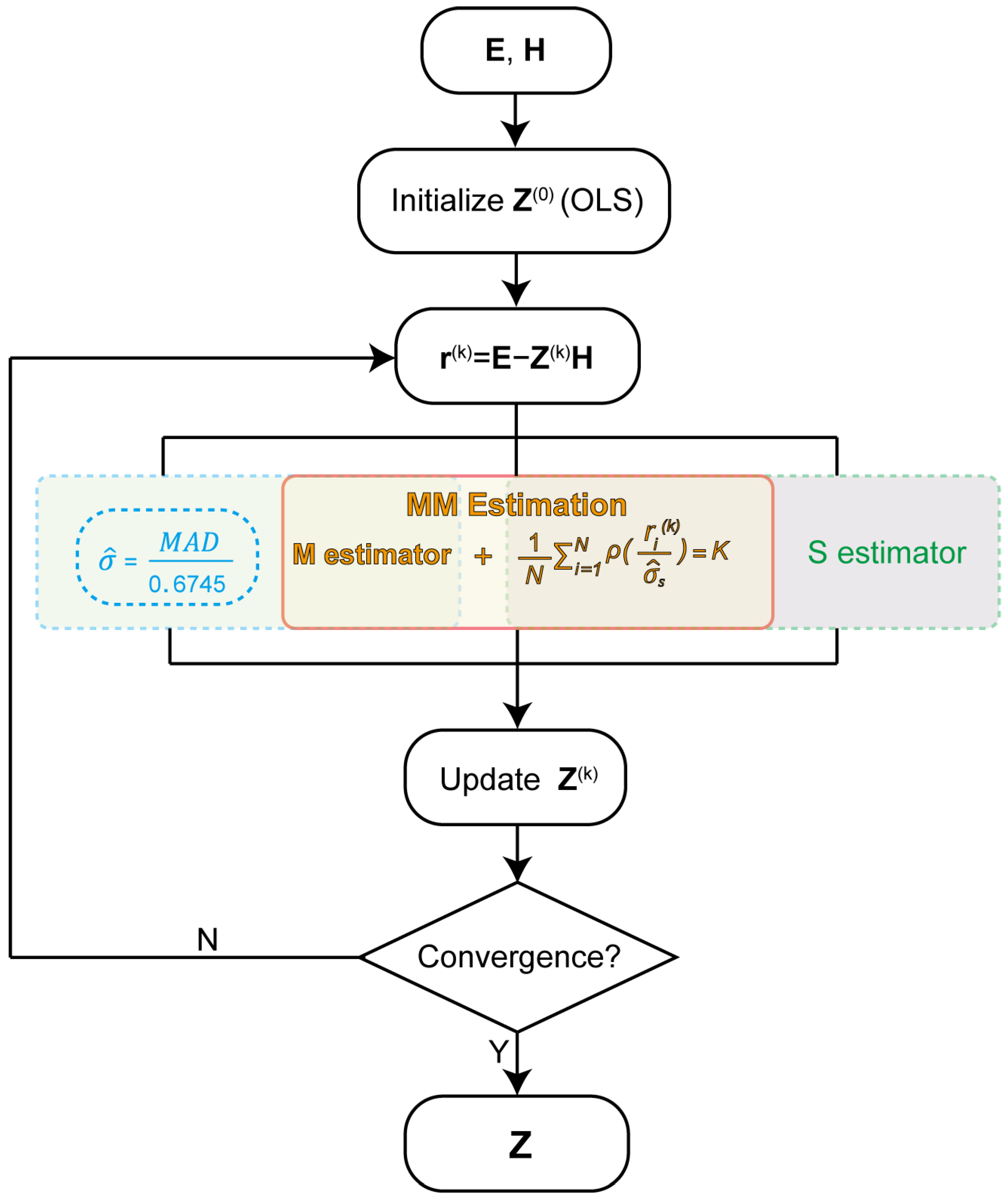
Figure 1. Flowchart of the M-, S-, and MM-estimation methods. OLS means ordinary least squares.
Minerals 16 00824 g001
Figure 2. Distribution of noise-contaminated samples over the full 10-day time series. The four noise components (Gaussian, square, peak, and sawtooth noise) were combined into a mixed-noise sequence and randomly added to selected samples. The vertical axis denotes the number of contaminated samples per 1000 data points.
Minerals 16 00824 g002
Figure 3. Comparison of clean and noise-contaminated EM time series at an SNR of 30 dB. Fifteen-minute data segments from Day Five are displayed as representative examples selected from a total of 10-day EM time-series dataset. Panels (a), (b), and (c) represent segments with 30%, 50%, and 70% of samples randomly contaminated by mixed noise, respectively (see Table 1 for parameter details). The orange and blue lines represent clean and noise-contaminated time series, respectively.
Minerals 16 00824 g003
Figure 4. Apparent resistivity and phase results estimated using M-estimator, S-estimator, and MM-estimator under mixed-noise contamination at an SNR of 30 dB. Panels (a), (b), and (c) show results for segments where 30%, 50%, and 70% samples were randomly contaminated by mixed noise (parameters listed in Table 1), respectively. The circles indicate apparent resistivity and phase calculated from the estimated impedance tensor, and error bars (1.96 σ) were computed from the standard errors of the impedance tensor components by the error propagation laws using the first-order Taylor expansion. The dashed line represents the theoretical response of the homogeneous half-space model.
Minerals 16 00824 g004
Figure 5. Distributions of deviations and normalized RMS errors for apparent resistivity and phase estimates obtained using M-estimator, S-estimator, and MM-estimator under mixed-noise contamination at an SNR of 30 dB. Panels (a), (b), and (c) illustrate frequency-dependent deviations of apparent resistivity and phase for noise contamination proportions of 30%, 50%, and 70%, respectively. Within each column, panels (a1c1) show deviations of apparent resistivity in the xy mode; panels (a2c2) show deviations of apparent resistivity in the yx mode; panels (a3c3) show deviations of phase in the xy mode; and panels (a4c4) show deviations of phase in the yx mode. Panels (d1d3) summarize the normalized RMS values for each method across the three contamination scenarios.
Minerals 16 00824 g005
Figure 6. Relative complex impedance errors obtained using M-estimator, S-estimator, and MM-estimator with respect to the theoretical half-space impedance under mixed-noise contamination at an SNR of 30 dB. Panels (a), (b), and (c) illustrate relative complex impedance errors for noise contamination proportions of 30%, 50%, and 70%, respectively. Within each column, panels (a1c1) show relative complex impedance errors in the xy mode; panels (a2c2) show relative complex impedance errors in the yx mode.
Minerals 16 00824 g006
Figure 7. Distributions of Total Error for apparent resistivity and phase estimates obtained using M-estimator, S-estimator, and MM-estimator under mixed-noise contamination at an SNR of 30 dB. Panels (a), (b), and (c) illustrate frequency-dependent Total Error of apparent resistivity and phase for noise contamination proportions of 30%, 50%, and 70%, respectively. Within each column, panels (a1c1) show the Total Error of apparent resistivity in the xy mode; panels (a2c2) show the Total Error of apparent resistivity in the yx mode; panels (a3c3) show the Total Error of phase in the xy mode; and panels (a4c4) show the Total Error of phase in the yx mode.
Minerals 16 00824 g007
Figure 8. Polar plots of the final weights of impedance tensor estimates at approximately 181 s under three contamination cases at an SNR of 30 dB, obtained using M-estimator, S-estimator, and MM-estimator. Panels (a), (b), and (c) correspond to contamination levels of 30%, 50%, and 70%, respectively (see Table 1 for noise parameters). Within each column, panels (a1c1) show results of M-estimator; panels (a2c2) show results of S-estimator; and panels (a3c3) show the results of MM-estimator. The radial distance denotes impedance magnitude, while the azimuthal angle represents impedance phase. The color intensity indicates the robust weight assigned to each estimate in the final iteration, with darker colors representing higher weights and lower residual influence.
Minerals 16 00824 g008
Figure 9. Comparison of clean and noise-contaminated EM time series at an SNR of 5 dB. Fifteen-minute data segments from Day Five are displayed as representative examples selected from the total 10-day EM time-series dataset. Panels (a), (b), and (c) represent segments with 30%, 50%, and 70% of samples randomly contaminated by mixed noise, respectively (see Table 1 for parameter details). The orange and blue lines represent clean and noise-contaminated time series, respectively.
Minerals 16 00824 g009
Figure 10. Apparent resistivity and phase results estimated using M-estimator, S-estimator, and MM-estimator under mixed-noise contamination at an SNR of 5 dB. Panels (a), (b), and (c) show results for segments where 30%, 50%, and 70% samples were randomly contaminated by mixed noises (parameters listed in Table 1), respectively. The error bars (1.96 σ) of the apparent resistivity and phase were computed from the standard errors of the impedance tensor components by the error propagation laws using the first-order Taylor expansion. The dashed line represents the theoretical response of the homogeneous half-space model.
Minerals 16 00824 g010
Figure 11. Distributions of deviations and normalized RMS errors for apparent resistivity and phase estimates obtained using M-estimator, S-estimator, and MM-estimator under mixed-noise contamination at an SNR of 5 dB. Panels (a), (b), and (c) illustrate frequency dependent deviations of apparent resistivity and phase for noise contamination proportions of 30%, 50%, and 70%, respectively. Within each column, panels (a1c1) show deviations of apparent resistivity in the xy mode; panels (a2c2) show deviations of apparent resistivity in the yx mode; panels (a3c3) show deviations of phase in the xy mode; and panels (a4c4) show deviations of phase in the yx mode. Panels (d1d3) summarize the normalized RMS values for each method across the three contamination scenarios.
Minerals 16 00824 g011
Figure 12. Relative complex impedance errors obtained using M-estimator, S-estimator, and MM-estimator with respect to the theoretical half-space impedance under mixed-noise contamination at an SNR of 5 dB. Panels (a), (b), and (c) illustrate relative complex impedance errors for noise contamination proportions of 30%, 50%, and 70%, respectively. Within each column, panels (a1c1) show relative complex impedance errors in the xy mode; panels (a2c2) show relative complex impedance errors in the yx mode.
Minerals 16 00824 g012
Figure 13. Distributions of Total Error for apparent resistivity and phase estimates obtained using M-estimator, S-estimator, and MM-estimator under mixed-noise contamination at an SNR of 5 dB. Panels (a), (b), and (c) illustrate frequency dependent Total Error of apparent resistivity and phase for noise contamination proportions of 30%, 50%, and 70%, respectively. Within each column, panels (a1c1) show the Total Error of apparent resistivity in the xy mode; panels (a2c2) show the Total Error of apparent resistivity in the yx mode; panels (a3c3) show the Total Error of phase in the xy mode; and panels (a4c4) show the Total Error of phase in the yx mode.
Minerals 16 00824 g013
Figure 14. Polar plots of the final weights of impedance tensor estimates at approximately 181 s under three contamination cases at an SNR of 5 dB, using M-estimator (left column), S-estimator (middle column), and MM-estimator (right column). Panels (a), (b), and (c) correspond to contamination levels of 30%, 50%, and 70%, respectively (see Table 1 for noise parameters). Within each column, panels (a1c1) show results of M-estimator; panels (a2c2) show results of S-estimator; and panels (a3c3) show the results of MM-estimator. The radial distance denotes impedance magnitude, while the azimuthal angle represents impedance phase. The color intensity indicates the robust weight assigned to each estimate in the final iteration with darker colors representing higher weights and lower residual influence.
Minerals 16 00824 g014
Figure 15. Schematic diagram of the profile location (after reference [63]). The red dashed line indicates the profile location, black filled triangles denote the stations used in this study, red filled squares represent cities, and black lines indicate faults.
Minerals 16 00824 g015
Figure 16. Comparison of apparent resistivity and impedance phase curves for station 520. Four estimation approaches are compared: remote reference method combined with M-estimator (RR), and local M-estimator, local S-estimator, and local MM-estimator. The remote reference station (500) was located approximately 15 km from local station 520. The error bars (1.96 σ) of the apparent resistivity and phase were computed from the standard errors of the impedance tensor components by the error propagation laws using the first-order Taylor expansion.
Minerals 16 00824 g016
Figure 17. Comparison of apparent resistivity and impedance phase curves for station 700. Four estimation approaches are compared: remote reference method combined with M-estimator (RR), local M-estimator, local S-estimator, and local MM-estimator. The remote reference station (690) was located approximately 12 km from local station 700. The error bars (1.96 σ) of the apparent resistivity and phase were computed from the standard errors of the impedance tensor components by the error propagation laws using the first-order Taylor expansion.
Minerals 16 00824 g017
Figure 18. RMS errors as a function of contamination level and SNR for M-, S-, and MM-estimator, respectively. Results were calculated with the synthetic datasets. Solid lines indicate results at SNR = 5 dB, whereas dashed lines illustrate results at SNR = 30 dB.
Minerals 16 00824 g018
Table 1. Parameters of different superimposed synthetic noise. Parameter α denotes the amplitude coefficient.
Noise TypesNoise AmplitudeOccurrence ProbabilityPeriod(s)Duty Cycle (%)
Gaussian 0.2 × α ---
Square 1.5 × α -30050
Peak 6.0 × α 2 × 10 5 --
Sawtooth 1.0 × α -20050
Table 2. Acquisition parameters of the MT stations used for field-data evaluation.
StationRoleLatitudeLongitudeElevation(m)Magnetic Coils
520Local43°23′53″ N122°45′30″ E180362/363/364
500Remote reference43°29′21″ N122°35′49″ E172348/360/361
700Local42°39′46″ N124°46′37″ E250348/360/361
690Remote reference42°42′14″ N124°38′49″ E240362/363/364
Disclaimer/Publisher’s Note: The statements, opinions and data contained in all publications are solely those of the individual author(s) and contributor(s) and not of MDPI and/or the editor(s). MDPI and/or the editor(s) disclaim responsibility for any injury to people or property resulting from any ideas, methods, instructions or products referred to in the content.