
Article

Geological and Alteration Mapping of Pit Walls at Gold Bar Mine Using Data-Driven Classification of Hyperspectral Imaging


by
Mehdi Abdolmaleki
1,
Trevor Robaldo
2,
Juan Carlos Ordóñez-Calderón
3 and
Kamran Esmaeili
1,*
1
Department of Civil and Mineral Engineering, University of Toronto, Toronto, ON M5S 1A4, Canada
2
McEwen Inc., 150 King St. West, Suite 2800, Toronto, ON M5H 1J9, Canada
3
Kinross Gold Corporation, 25 York St., Toronto, ON M5J 2V5, Canada
*
Author to whom correspondence should be addressed.
Minerals 2026, 16(8), 816; https://doi.org/10.3390/min16080816
Submission received: 10 June 2026 / Revised: 15 July 2026 / Accepted: 4 August 2026 / Published: 6 August 2026

Abstract

In open-pit mining, accurately mapping lithology, alteration, and mineralogy is vital for optimizing ore grade estimation, processing, and operational planning. Traditional geological pit-wall mapping is time-consuming, labor-intensive, and exposes technical staff to hazardous conditions. This study investigates a data-driven, hyperspectral classification workflow for pit-wall mapping at an open-pit gold mine. Three classification techniques were applied: Spectral Angle Mapper (SAM) using scene-derived reference spectra, Autoencoder + K-means (AE), and Band Ratio + K-means (BR), without relying on predefined training labels. Hyperspectral imagery was acquired using a tripod-mounted system integrating VNIR (400–1000 nm) and SWIR (970–2500 nm) sensors from two pit walls of contrasting geological complexity, with SWIR data driving primary mineral classification and VNIR data used separately for iron oxide mapping. Results were validated against laboratory hyperspectral scanning and XRD analyses of collected rock samples, as well as expert geological interpretation. Across both pit walls, Across both pit walls, SAM and BR produced closely consistent, geologically reliable classifications, with SAM showing the strongest correspondence to reference spectra and confirmed mineral assemblages; AE achieved comparable polygon-level agreement but with reduced mineralogical specificity, tending toward broader, less distinct class groupings. The study demonstrates that close-range tripod-based hyperspectral imaging with data-driven classification provides a practical, rapid alternative to manual pit-wall mapping, improving accuracy, reducing interpretation time, and minimizing personnel exposure to hazardous conditions.

1. Introduction

In a mining operation, identifying and characterizing the geological features that control the distribution of ore grades and minerals is essential for optimizing the exploitation process and production planning. It is essential that any variation in lithology, alteration, mineralogy, and structures exposed at the mine faces be identified and mapped, as it can significantly influence mine production performance and efficiency in terms of the quantity and quality of the produced ore, as well as the cost, time, and method of mineral processing. Therefore, all geological models and operational plans should be continually updated throughout the life of a mine by acquiring and integrating new geological data. In this regard, using an efficient, rapid, and accurate geological data acquisition approach along with a precise and automated decision-making system is crucial for the mining industry. Such a system would allow for the detection and characterization (quantitatively and qualitatively) of different geological features [1,2]. Geological mapping involves recording and gathering all relevant data from a mine site to evaluate and analyze geological features, including lithological units, major structures, and alteration zones, and their spatial distributions [1]. Traditional pit wall mapping in mining operations, often undertaken to support grade control and geological interpretation, is typically performed manually by geologists. Although effective, this approach is time-consuming, labor-intensive, and may expose personnel to potentially hazardous working conditions. Mines with a high rate of production and development, or with a large area of operational activities, need to collect and analyze a large amount of geological data and update the mine geological and structural models and operational plans in a short amount of time. This requires considerable manpower to collect and analyze the necessary data to update the models. This is particularly important for remote mine sites, which rely on limited staff resources. In addition, conventional mapping techniques can expose technical staff to numerous risks, including falling rock blocks, moving equipment, pit wall failure, and exposure to dust and gases. Moreover, acquiring data from some inaccessible locations (for either safety or logistical reasons) is not possible by conventional methods [1,3,4,5,6].
Remote sensing data and digital imagery have significantly enhanced pit wall mapping in open-pit operations [7,8]. Both aerial (UAV) and terrestrial remote sensing techniques have been successfully used for data acquisition, providing high-resolution imagery with reduced proximity requirements and shorter equipment setup times, thereby improving mapping efficiency and minimizing logistical challenges associated with conventional approaches [8]. Recent studies have demonstrated successful integration of remote sensing and machine learning for automated geological and structural mapping. Automated mapping systems offer significant benefits for operations, enhancing efficiency, accuracy, and safety while reducing reliance on manual fieldwork [9,10,11].
While RGB imaging and photogrammetry have been widely used to visualize and analyze lithology and structure, and for automated geological mapping [8,12,13,14,15,16,17,18], these methods are fundamentally constrained by their reliance on three broad visible-light bands, which limits their ability to detect the subtle compositional and alteration differences that govern ore quality and mineral assemblage in active mining environments [19]. In contrast, hyperspectral imagery captures hundreds of contiguous spectral bands across the VNIR (400–1000 nm) and SWIR (1000–2500 nm) ranges, enabling identification of diagnostic absorption features associated with clay minerals, iron oxides, carbonates, and sulphates, mineral groups of direct relevance to ore deposit characterization and alteration mapping [20,21,22,23]. This spectral richness makes hyperspectral imaging particularly well-suited to pit-wall environments, where compositionally similar lithologies must be distinguished at fine spatial scales, decimeter- to meter-scale variability along exposed pit walls that may be smaller than the support of routine geological mapping or mining blocks but still influence local ore–waste boundaries, alteration interpretation, and where surface alteration patterns directly inform ore grade estimation and processing decisions. Recent reviews have further demonstrated the value of hyperspectral data for mine-scale geological mapping, including applications to open-pit faces, blasted rock piles and underground mine walls [24,25,26].
Extensive research has examined the application of hyperspectral remote sensing to surface geological mapping and mineral identification [27,28,29,30,31,32,33]. A growing body of work has specifically investigated hyperspectral imaging in steep and vertical geological exposures relevant to mining and geotechnical applications. Fraser et al. (2006) [34] emphasized the importance of in situ hyperspectral data for geological identification on mine faces, which is essential for automating exploration and ore grading. Kurz et al. (2012) [35] demonstrated that compact, close-range hyperspectral imagers can achieve high spatial resolution and optimal viewing geometry on quarry walls and steep cliff sections. Thiele et al. (2021) [36] extended this to UAV-mounted systems, proposing correction methodologies for precise hyperspectral acquisition on vertical cliff faces and demonstrating effective geological facies mapping. Boubanga-Tombet et al. (2018) [37] further showed that lightweight thermal infrared hyperspectral instruments can resolve fine-scale mineralogy and lithology in vertical cliff sections at high spectral and spatial resolution. Despite this progress, the specific operational context of active open-pit mine face mapping with hydrothermal alteration assemblages has received comparatively less systematic attention than lithological mapping in quarry or natural cliff settings. While studies such as Booysen et al. 2022 [38] and Kirsch et al. 2018 [19] have demonstrated the value of integrating close-range terrestrial hyperspectral scanning with laboratory sample analysis in mining environments, these have focused on lithium-pegmatite (Uis, Namibia) and polymetallic vein-hosted hydrothermal (Freiberg, Germany) systems, respectively, rather than Carlin-type sediment-hosted gold deposits, where fine-scale alteration zonation, including clay mineral assemblages, iron oxides, and carbonate distributions, directly controls ore grade. Furthermore, systematic comparative evaluation of multiple data-driven classification approaches, spanning conventional spectral matching, band ratio analysis, and deep learning-based feature extraction, applied to pit walls of contrasting geological complexity and cross-validated against laboratory hyperspectral scanning and XRD mineralogy of collected rock samples, remains limited in the published operational literature.
This study addresses these gaps by presenting an operational hyperspectral imaging and classification workflow for geological and alteration mapping at the Gold Bar open-pit gold mine in Nevada, USA. Rather than introducing new classification algorithms, the contribution of this study lies in the systematic comparison of three complementary unsupervised hyperspectral classification approaches within a single operational framework and their evaluation under contrasting geological conditions. Hyperspectral data were acquired using a tripod-mounted HySpex Mjolnir VS-620 system integrating both VNIR (400–1000 nm) and SWIR (970–2500 nm) sensors, with VNIR data used for iron oxide discrimination and SWIR data used for the primary lithological and alteration classification. Building on a previous study by our research group that employed UAV-mounted RGB imaging for pit-wall mapping [8], the present work extends that approach by incorporating full hyperspectral characterization, enabling mineral discrimination and alteration mapping beyond the capability of RGB imagery. Three data-driven, classification techniques are evaluated: Spectral Angle Mapper (SAM), a reference-based spectral matching method in which endmember are extracted directly from the hyperspectral scene using the Pixel Purity Index algorithm without reliance on external spectral libraries; Autoencoder combined with K-means clustering (AE), which explores whether deep learning latent representations improve geological separability; and Band Ratio (BR) with K-means, which emphasizes diagnostic mineralogical contrasts through spectral indices. A further contribution of this study is the comprehensive validation framework, in which classification results are cross-validated using laboratory hyperspectral scanning, XRD mineralogical analysis of collected rock samples, local spectral references, and expert geological interpretation, providing a direct laboratory-to-field spectral correspondence that has rarely been reported for operational pit-wall hyperspectral mapping. Finally, the study evaluates how classification performance and geological interpretability vary between structurally simple and complex pit-wall settings, providing practical guidance for selecting appropriate classification methods for geological mapping in active mining environments.

2. Previous Work: Pit Wall Mapping Using UAV-Mounted RGB Imaging

A previous study [8] focused on pit wall mapping at two open-pit mines in Nevada, specifically the Bald Mountain Mine (Top Pit), Kinross Gold Corporation, and the Gold Bar Mine (Pick Pit), McEwen Mining Inc., using UAV-mounted RGB imaging. Data were collected with a DJI Inspire 2 UAV (DIJ, Shenzhen, China) equipped with a Zenmuse X5S camera. High-resolution RGB images were processed using photogrammetry to generate 3D point clouds and orthomosaics. Ground-truth labels for geological units were provided by senior mine geologists.
The study employed an unsupervised learning approach based on stacked autoencoders for feature extraction and dimensionality reduction, followed by K-Means clustering for geological unit classification. The autoencoder was trained on image tiles ranging from 64 × 64 to 256 × 256 pixels, and the extracted features were embedded with t-SNE before clustering. The results showed that the methodology performed well in the Top Pit, achieving an overall classification accuracy of 75.8%, with individual unit F1 scores ranging from 70% to 82%. However, at the Pick Pit, which exhibited a more complex geological distribution, accuracy dropped to 55%, with F1 scores ranging from 29% to 69%.
The main limitation of the study was reliance on RGB imaging, which lacks the spectral information required for precise mineral discrimination. Classification was based solely on color variations, leading to misclassification in areas with subtle lithological differences. These findings underscored the need for more advanced spectral techniques, such as hyperspectral imaging, to improve geological unit discrimination. The insights from this study formed the basis for the current research, which aims to enhance pit wall mapping through hyperspectral imaging and a broader range of classification techniques. Further details on the methodology and results of the previous work can be found in Yang et al. (2023) [8].

3. Study Area and Data Collection

3.1. Study Area: Gold Bar Mine

The study area, located at McEwen Mining’s Gold Bar mine (39°47′ N, 116°20′ W, WGS 84) near Eureka, Nevada, offers a rich geological setting with gold mineralization in thin-bedded carbonate rocks (Figure 1). Mineralization at the site is influenced by structural conduits trending northwest and northeast, and ore types include oxidized, jasperoidal, and carbonaceous ore, predominantly associated with sulfides. The sedimentary rock formations in the area, such as the McColley Canyon Formation and Denay Formation, exhibit varying degrees and types of alteration. The mineralization is largely oxidized and linked to decarbonatized and argillized carbonate debris-flows and turbidites, with illite clays prevalent in mineralized zones alongside other clay species such as kaolinite and dickite. Silicification is notable in the district, with specific generations associated with gold mineralization. Unoxidized zones are characterized by carbonaceous material and may contain significant gold mineralization alongside minerals such as orpiment, realgar, and fine-grained pyrite.

3.2. Hyperspectral Data COLLECTION

For this study, hyperspectral imaging (HIS) was conducted on two pit walls at the Gold Bar Mine: the West Wall in Gold Bar South and Pick 3 in Gold Bar North. A tripod-mounted HySpex Mjolnir VS-620, Neo, Oslo, Norway, hyperspectral imaging system was used, integrating VNIR and SWIR sensors to capture spectral information across 400–2500 nm. VNIR data were specifically used for iron oxide discrimination, while SWIR data drove the primary lithological and alteration classification. The scanning process involved optimizing the integration time, adjusted iteratively based on test scans of the Spectralon® (Labsphere Inc) reference panels and the pit wall surface to avoid sensor saturation in bright areas while maintaining sufficient signal-to-noise ratio across the scene, and performing radiometric calibration. White reflectance panels were used in the field to calibrate reflectance. Deploying such panels may not always be feasible in inaccessible or hard-to-reach areas. In such cases, alternative approaches can be used, such as reference spectra or software-based correction methods specifically designed for ground-based scanning geometries, such as DROACOR [40], which account for illumination and sensor-specific effects in close-range acquisitions. Sensor specifications are listed in Table 1.
It should be clarified that the primary lithological and alteration classification (SAM, AE, and BR) presented in this study is based entirely on the SWIR sensor; the VNIR sensor was used only for a separate, independent iron oxide classification. The VNIR and SWIR spectral datasets were processed independently within separate workflows, without cross-band data fusion at the raw radiance or reflectance level. For final map integration, the two independent classification outputs were spatially aligned using prominent, mutually identifiable topographic features on the pit wall, and the higher-resolution VNIR classification output was resampled using nearest-neighbor assignment to match the spatial grid layout of the SWIR-based maps. This co-registration procedure enabled spatial comparison between the SWIR-derived mineralogical units and the VNIR-derived iron oxide distribution without altering the underlying independent analyses.
At the West Wall, the hyperspectral camera was positioned at a height of 181 cm, with a scanning distance of 40 m from the wall and a rotational speed of 3 radians per minute, yielding a SWIR ground sampling distance of approximately 2.2 cm/pixel and a vertical wall coverage of approximately 13.4 m based on the sensor’s 20° field of view. For Pick 3, the camera was set at a height of 144 cm, with a significantly greater scanning distance of 150 m and the same rotational speed, yielding a SWIR ground sampling distance of approximately 8.1 cm/pixel and a theoretical vertical coverage of approximately 53 m. In both cases, calibration was performed using two Spectralon® white reflectance panels (50 cm × 50 cm) with reflectance levels of 20% and 50%.
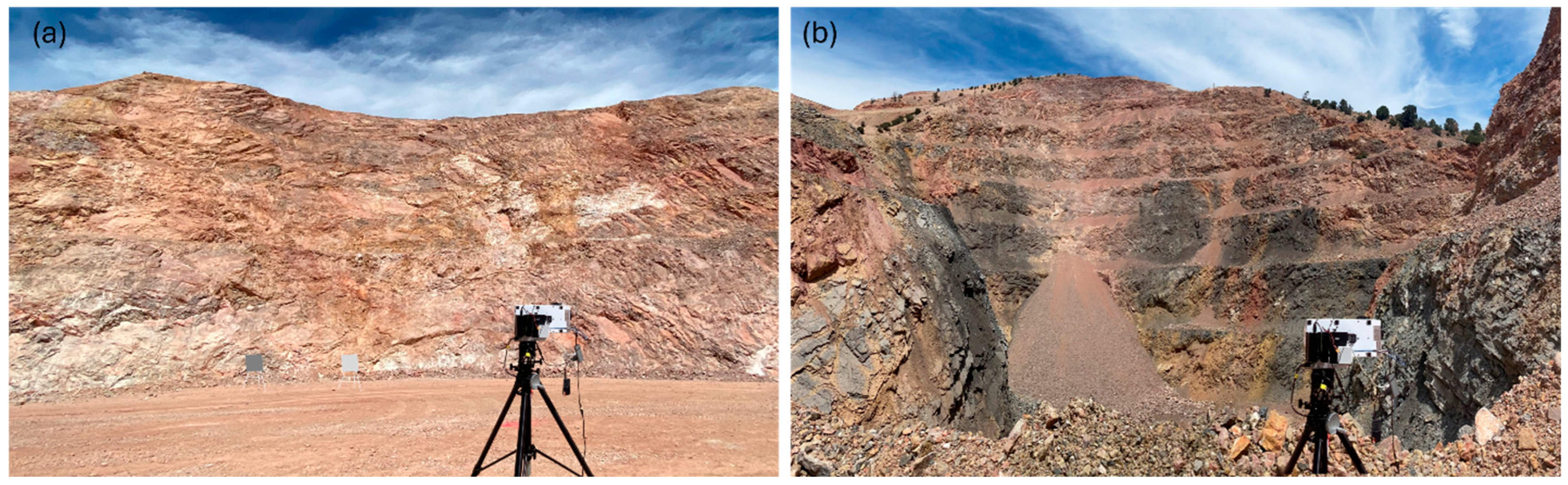
Data acquisition took place under natural sunlight on a clear day. The West Wall was scanned at noon (12:00 PM) to take advantage of near-overhead illumination, minimizing directional shadows on the wall face. The Pick 3 wall was scanned at 3:00 PM, when the westerly sun angle provided more direct illumination on the predominantly east-facing wall surface; this timing also aligned with site access and equipment setup constraints. Setting up the tripod and scanner took approximately 15 min, while each hyperspectral scan took under 1 min, depending on the rotation speed and field of view. For example, one scan of the West Wall pit wall, with a Frame period of 10,000 µs and 1939 frames, resulted in a total scan time of approximately 20 s, corresponding to a rotation speed of 3 degrees/second and a field of view of 60°. Figure 2 illustrates the field setup for hyperspectral imaging at both walls.

3.3. Reference Data for Labeling

To accurately label the hyperspectral images obtained from field scanning, two primary sources of reference data were utilized: local reference spectra and laboratory-analyzed rock samples. These datasets provided essential validation and enabled meaningful geological and mineralogical interpretations of the resulting spectral clusters, which will be generated using unsupervised classification techniques described in the following methodology section.

3.3.1. Reference Linking and DOIs

The local spectral library was compiled from a spectral analysis report on the Gold Bar mine [41]. A total of 15 reference spectra were extracted from this report. These spectra were initially collected using a Terraspec spectrometer, ADS Inc., Louisville, CO, USA, from chip trays, chipboards, and core samples at the mine site. To ensure maximum ground-truth fidelity and eliminate ambiguity in automated outputs, the spectral labels in this reference library were explicitly assigned through expert geological review using The Spectral Geologist (TSG8) and SpecMin software packages (3.1). Mineral dominance and class labeling were determined strictly by diagnostic absorption-feature positions. These interpretations were further cross-verified and supported by extensive field validation, historical drill logs, chemical assay data, and systematic refinement against custom, site-specific spectral controls [41].
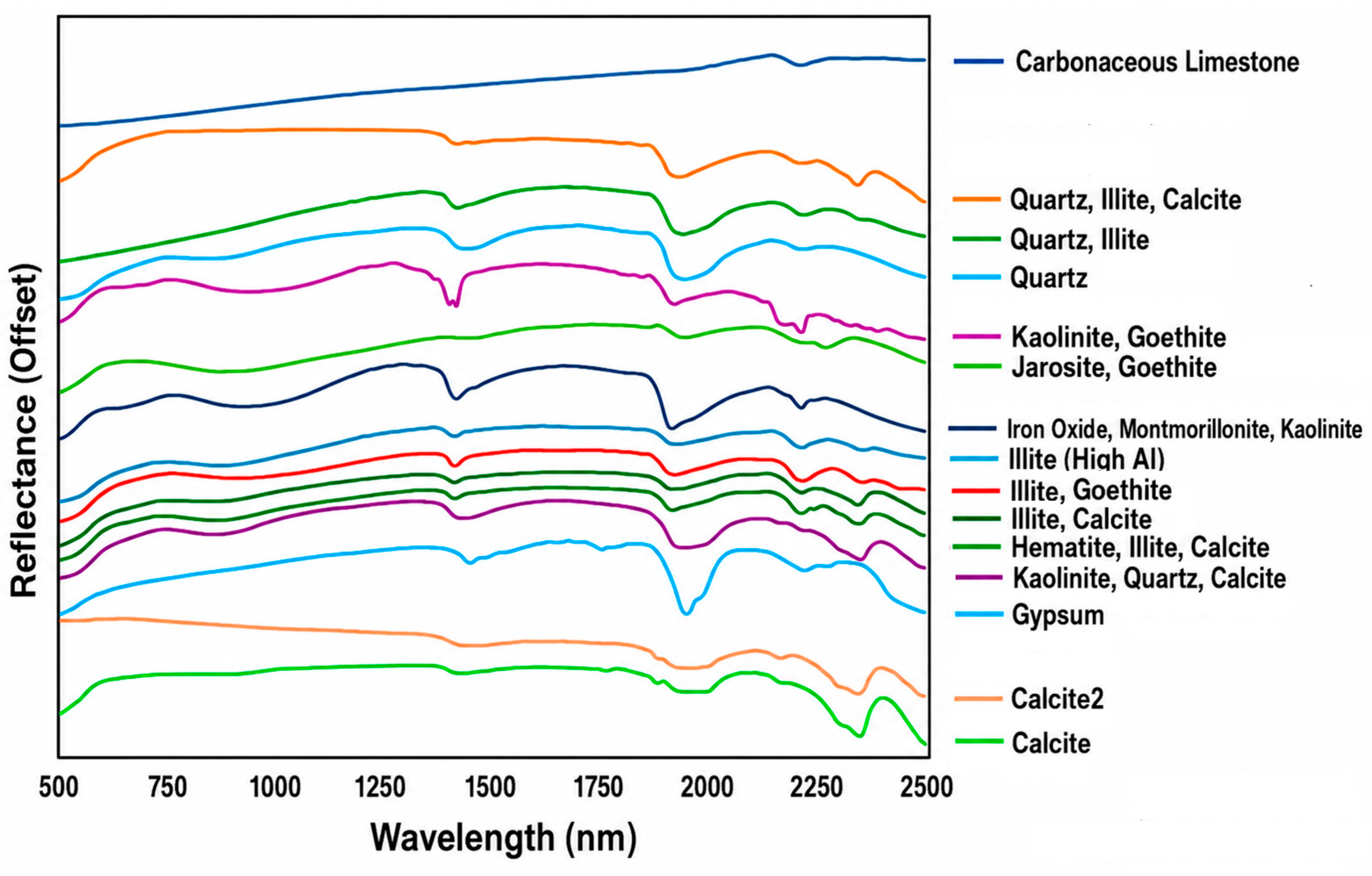
The spectral data primarily indicated the presence of clay, quartz, and carbonate minerals, which are key indicators of geological variation. Additionally, carbonaceous limestone was identified, which is particularly significant due to its role in preg-robbing during gold leaching, potentially reducing recovery efficiency. To ensure spectral compatibility with the HySpex Mjolnir VS-620 imaging system used for pit wall scanning, the local spectra were resampled to match the HySpex system’s characteristic band intervals and band count. This resampling was performed in ENVI (V6.2) using a Gaussian spectral response function (SRF) convolution algorithm based on the center wavelengths and Full Width at Half Maximum (FWHM) specifications of the HySpex sensor, Neo, Oslo, Norway. This approach accurately simulates the target instrument’s actual spectral response and prevents artificial shifting or flattening of critical mineral features. This step ensured consistent spectral resolution, enabling accurate comparisons and assessments of similarity. These local spectra were used to match and interpret clusters obtained from post-processing of hyperspectral data. Figure 3 presents the local spectral library used in this study. It should be noted that these spectra were collected from locations in close proximity to the Pick 3 pit wall, representing the same hydrothermal alteration system and mineral assemblages present there. They were therefore used as a primary reference for interpreting Pick 3 classification outputs. For the West Wall, however, the geological conditions differ substantially from the areas represented by this spectral library, and accordingly, these spectra were not applied as a validation source for that wall; West Wall outputs were instead assessed through expert geological interpretation, as described in Section 5.2.

3.3.2. Hyperspectral Scanning of Rock Samples

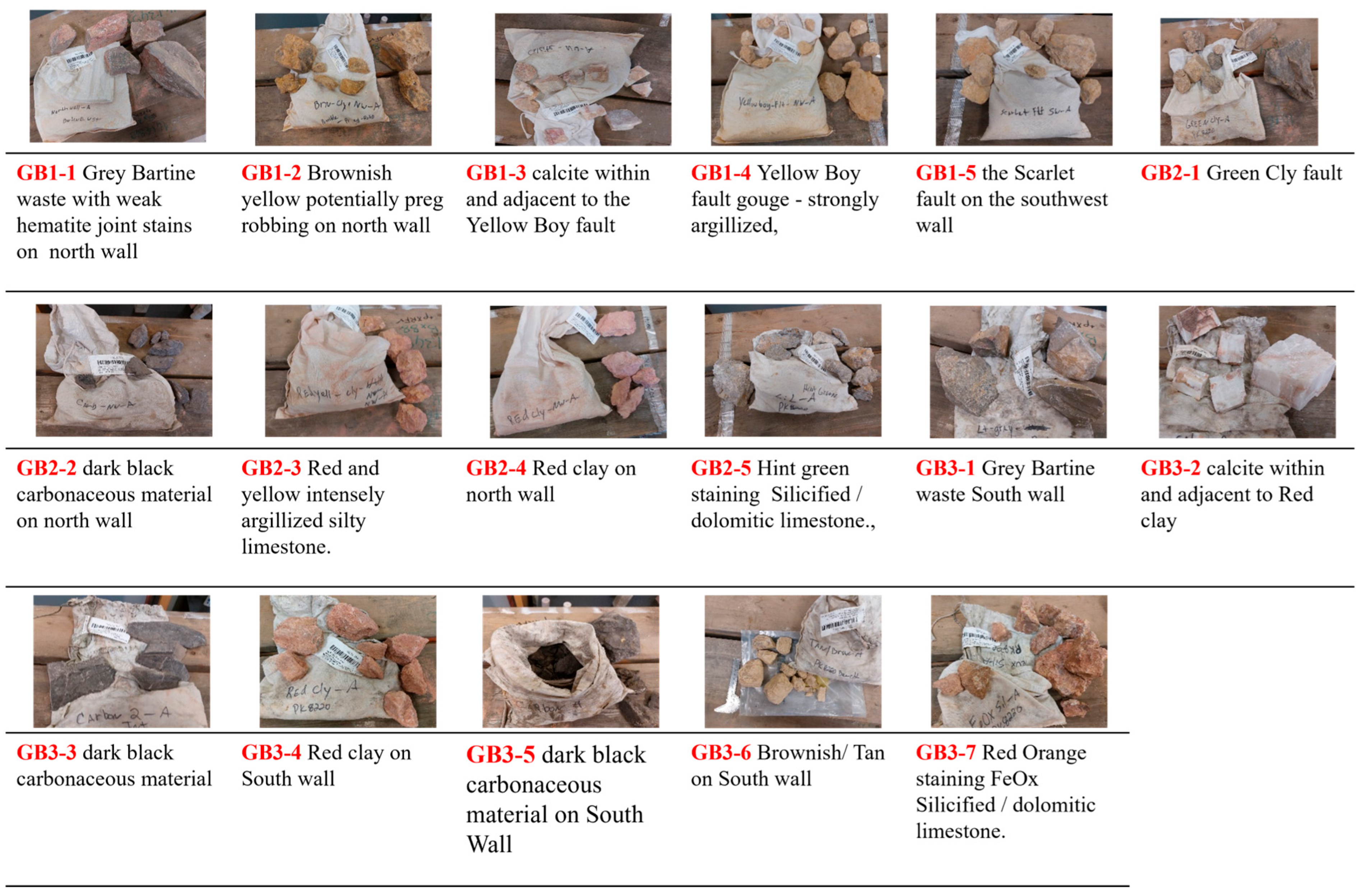
In the 2022 study at Gold Bar Mine (mainly focused on Gold Bar north), 17 rock sample bags, each weighing 3 to 5 kg, were collected from pit walls. Each bag contained multiple hand-sized rock fragments representing various geological units and alteration zones. All samples were scanned using the SisuRock hyperspectral system (manufactured by Specim, Spectral Imaging Ltd., Oulu, Finland) at the University of Alberta, equipped with Specim VNIR and Specim SWIR push-broom hyperspectral cameras, covering a broad reflectance range from 400 to 1000 nm in the VNIR and from 900 to 2500 nm in the SWIR. The scanner operated with an integration time of 2 ms. The VNIR sensor featured a physical spectral resolution (FWHM) of approximately 2.8 nm with a spectral sampling interval of ~6.8 nm across 88 bands, while the SWIR sensor featured a physical spectral resolution of 10 nm with a spectral sampling interval of ~6.25 nm across 256 bands. The spatial resolutions were set to 200 µm/pixel in the VNIR and 350 µm/pixel in the SWIR. To ensure spectral compatibility with the HySpex imaging system (used for fieldwork), the mean spectrum for each sample was calculated and then resampled to match the system’s requirements. For each of the 17 rock samples, all rock fragments contained within the sample bag were scanned on their natural, unprepared surfaces, and a single mean spectrum per sample was calculated by averaging the spectral responses across all fragments. These samples provided a direct reference for spectral comparison, enabling the validation and refinement of labels assigned to clusters derived from the post-processing of hyperspectral data. Figure 4 presents photographs and descriptions of the collected rock samples. The sample collection locations are in close proximity to the Pick 3 pit wall and represent the same lithological units and alteration zones present there, including clay mineral assemblages, iron oxides, carbonaceous limestone, and carbonate phases. As with the local spectral library, the geological conditions of the West Wall differ substantially from the areas where these samples were collected, and they were therefore not used for direct validation of West Wall classification outputs, which relied instead on expert geological interpretation.

3.4. XRD Analysis

Mineralogical analysis of 17 rock samples collected from the Gold Bar North area was performed using X-ray diffraction (XRD) to provide independent compositional characterization. Analyses were performed by SGS Natural Resources (Lakefield, ON, Canada) using a Bruker AXS D8 Advance diffractometer, Bruker Corp., Billerica, MA, USA, with Rietveld refinement (Topas 4.2), with a reported detection limit of 0.5%–2% depending on phase crystallinity. The results (Table 2) show the presence of quartz, calcite, dolomite, and muscovite, consistent with lithological features dominated by carbonate rocks, including limestones, dolomites, siliciclastic sediments, and their hydrothermally altered products. The presence of amorphous phases (up to ~23%) indicates poor crystallinity, most likely representing alteration products. Overall, the XRD results delineate a mineralogical trend from calcite/dolomite-dominated to quartz-rich compositions, representing the spectrum of chemical-siliciclastic rocks and hydrothermally altered products. Table 2 summarizes the quantitative XRD results for the analyzed rock samples.

4. Methodology

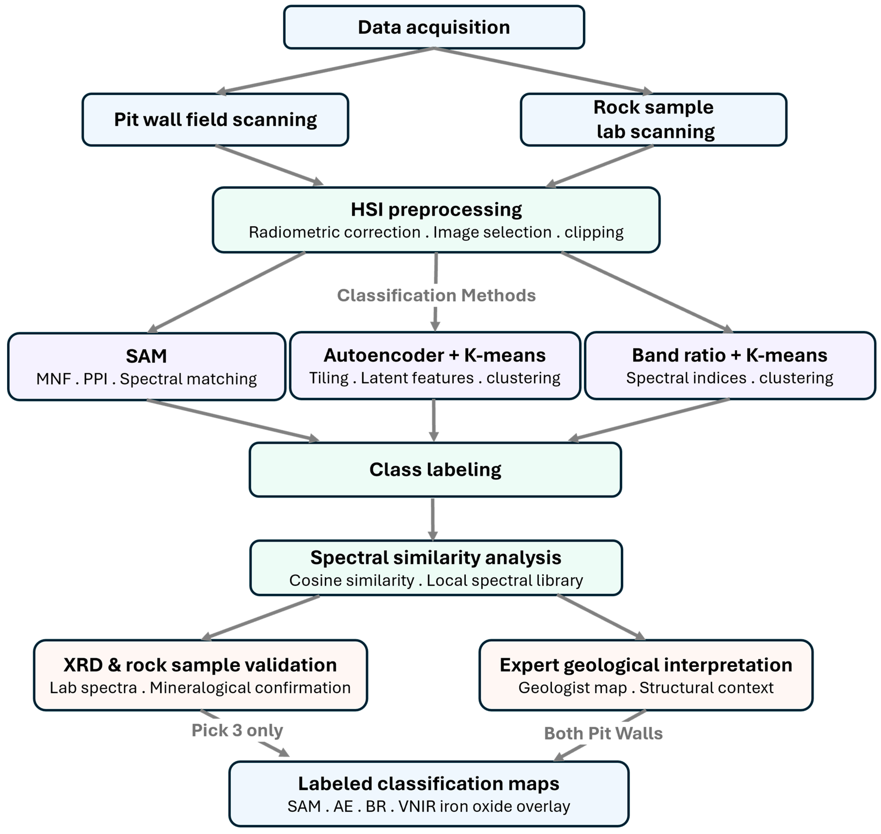
Figure 5 illustrates the overall workflow of this study, comprising several key stages, including hyperspectral data acquisition, preprocessing, classification, and spectral similarity analysis. In this section, the methodology is demonstrated using the Pick 3 dataset as an example; the same workflow was also applied to the West Wall data, with minor adjustments as needed. The process begins with the acquisition of hyperspectral data, including both lab-scale scanning of rock samples and field-scale scanning of pit walls at the Gold Bar mine. The lab-scale scanning of rock samples serves as a reference for subsequent spectral analysis and classification. Following data collection, hyperspectral image preprocessing is performed to enhance data quality and remove unwanted noise. This phase includes converting radiance images to reflectance using white reflectance calibration; excluding scan lines/frames affected by saturation, motion blur, or inconsistent illumination; reorienting images so that the along-track scanning direction is displayed left-to-right as collected, rather than top-to-bottom as per default software display conventions; extracting relevant regions by clipping; and removing spectral bands affected by atmospheric water vapor absorption (centered near 1400 nm, 1900 nm, and 2400 nm) as well as the outermost bands at the edges of the sensor’s spectral range, which characteristically exhibit reduced signal-to-noise ratio. The processed hyperspectral images are then analyzed using three data-driven classification techniques (SAM, AE, and BR).
The first approach, SAM, classifies pixels based on spectral similarity to reference spectra derived entirely from the hyperspectral scene itself using the Pixel Purity Index (PPI) algorithm, and geological labelling of the resulting classes was performed by domain geologists only after classification. The second technique, an autoencoder combined with K-Means clustering, applies deep learning to extract high-level spectral features, which are then clustered into distinct geological units. The third technique applies a knowledge-based band-ratio feature construction step, in which ratios were defined from expert-identified diagnostic absorption wavelengths in the local spectral library, followed by unsupervised K-means clustering of the resulting band-ratio images to delineate distinct geological/alteration units. We describe these three approaches collectively as a hybrid framework combining data-driven clustering with knowledge-based constraints. The classification steps themselves are data-driven, as the underlying algorithms (K-means and the autoencoder) operate purely on unlabeled pixel data without predefined training targets. However, expert geological input is intentionally integrated at key operational stages: first, via a knowledge-based feature construction step to select diagnostic wavelength pairs for BR; second, through the manual curation of scene-derived endmembers for SAM; and third, in the separate VNIR iron oxide mapping, which relies on an external reference library. Once classification is complete, the resulting numeric cluster IDs are relabeled with geological/mineral class names through a class-labeling step, in which each cluster’s spectral signature is compared against reference spectra from the local spectral library and from lab-scanned rock samples. This spectral similarity analysis enables the accurate identification and labeling of geological and alteration units within the scanned pit walls. The following sections provide a detailed discussion of each step, including data collection methodologies, preprocessing techniques, classification algorithms, and spectral analysis approaches.

4.1. Hyperspectral Image Preprocessing

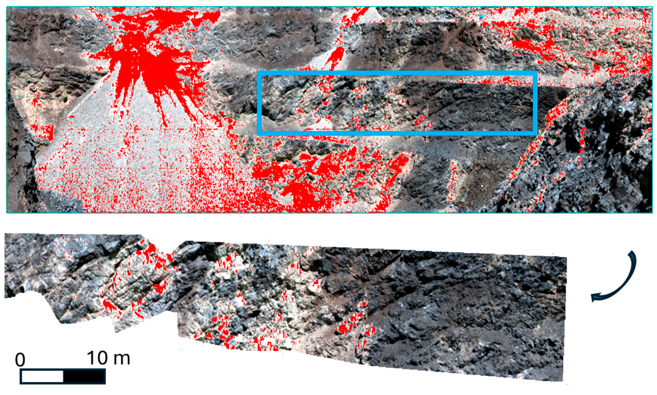
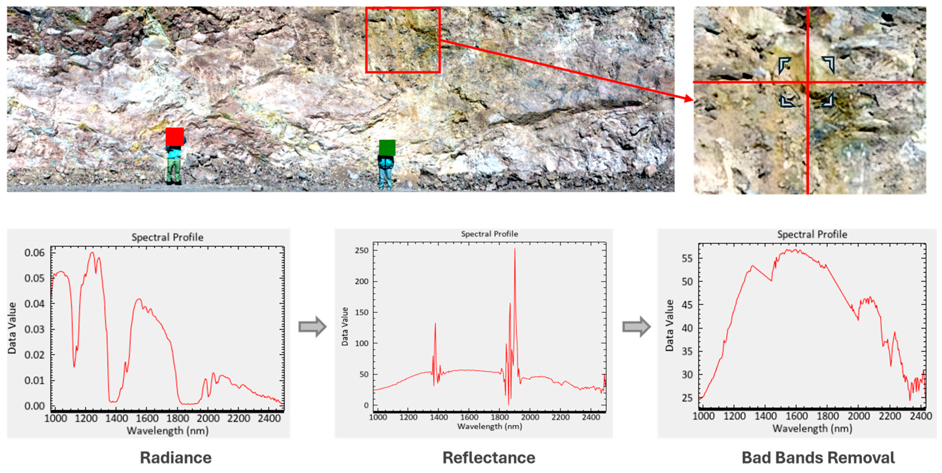
Before analysis, raw hyperspectral images underwent several preprocessing steps to ensure data quality and reliability, including radiance conversion, image selection, orientation correction, image clipping, reflectance transformation, and removal of noisy bands. Oversaturated regions were identified and masked prior to image clipping. Figure 6 shows the saturation analysis for Pick 3, with the selected analysis region indicated by the blue rectangle. The analysis region was selected using the saturation map (Figure 6) by identifying the area with the minimum extent of saturated pixels while still capturing a representative range of the geological and alteration units present on the pit wall. Pixels flagged as saturated (shown in red) indicate that one or more spectral bands exceeded the sensor’s dynamic range. This saturation was concentrated predominantly in the early SWIR range (around 1000–1300 nm) due to highly reflective sloughed material on the benches, leaving the diagnostic absorption features beyond 2000 nm fully intact. These affected pixels were masked and excluded from subsequent analysis. Reflectance conversion was performed using empirical line correction [43] with two Spectralon® white reflectance panels (20% and 50% nominal reflectance, 50 cm × 50 cm) deployed in the field during acquisition. To avoid mixed-pixel effects along the panel margins, a conservative region of interest (ROI) of approximately 460 pure pixels was extracted from the homogeneous center of each panel to calculate the average calibration coefficients. This approach contextualizes the spectral data by removing variations caused by atmospheric attenuation and changing illumination conditions, rendering the spectral features independent of environmental factors without requiring auxiliary atmospheric models or Digital Elevation Model (DEM)-based topographic corrections. Spectral bands heavily impacted by atmospheric water vapor absorption (centered around 1.4 µm and 2.0 µm) were subsequently masked and removed from further analysis due to severe signal attenuation.
Normalizing the data to surface reflectance provides a consistent basis for accurately distinguishing mineral species using diagnostic absorption features. Figure 7 illustrates the transition from raw radiance to relative surface reflectance and the effect of absorbing-band removal for the West Wall, highlighting how the corrected reflectance curves isolate the intrinsic material properties required for knowledge-based labeling and comparison against the mentioned local spectral libraries.
All subsequent classification methods (SAM, AE, and BR) received the same preprocessed reflectance data as input. Method-specific transformations, specifically MNF for SAM’s endmember extraction step, are described within their respective method sections.
With these preprocessing steps completed, the hyperspectral data are now fully prepared for further analysis, including classification and spectral similarity assessments. Depending on data volume and computational resources, the developed preprocessing workflow allowed each hyperspectral image to be processed in approximately 10–15 min, whereas step-by-step manual preprocessing required substantially more time.

4.2. Data-Driven Classification Techniques

4.2.1. Spectral Angle Mapper (SAM)

In this study, the SAM algorithm was employed to classify hyperspectral images by comparing spectral similarity to selected reference spectra. Before applying SAM, we implemented the Minimum Noise Fraction (MNF) transformation to reduce data dimensionality and enhance the signal-to-noise ratio [44]. MNF serves a dual role in this context: reducing noise and rotating the spectral data into a lower-dimensional space in which spectrally pure pixels can be reliably identified. This transformation was applied exclusively within the SAM workflow; AE and BR operated directly on the preprocessed reflectance bands, as the autoencoder architecture incorporates implicit noise suppression through its reconstruction objective, and band ratio computation relies on raw reflectance band values to preserve the spectral relationships between numerator and denominator bands. Following the MNF transformation, the Pixel Purity Index (PPI) method was used to identify spectrally pure pixels, commonly referred to as endmembers, within the hyperspectral dataset. These endmembers represent the most spectrally distinct signatures present in the image. This extraction framework represents a user-guided, data-driven approach rather than a strictly automated or unsupervised classification. Notably, a dedicated low-signal or shadow mask was not applied prior to running the PPI algorithm. Consequently, deep shadows and low-signal pixels with high geometric extremity in the MNF space were initially flagged by the algorithm. To resolve this, a manual visual inspection and filtering phase was required to purge these shadow artifacts before finalizing the mineral reference set.
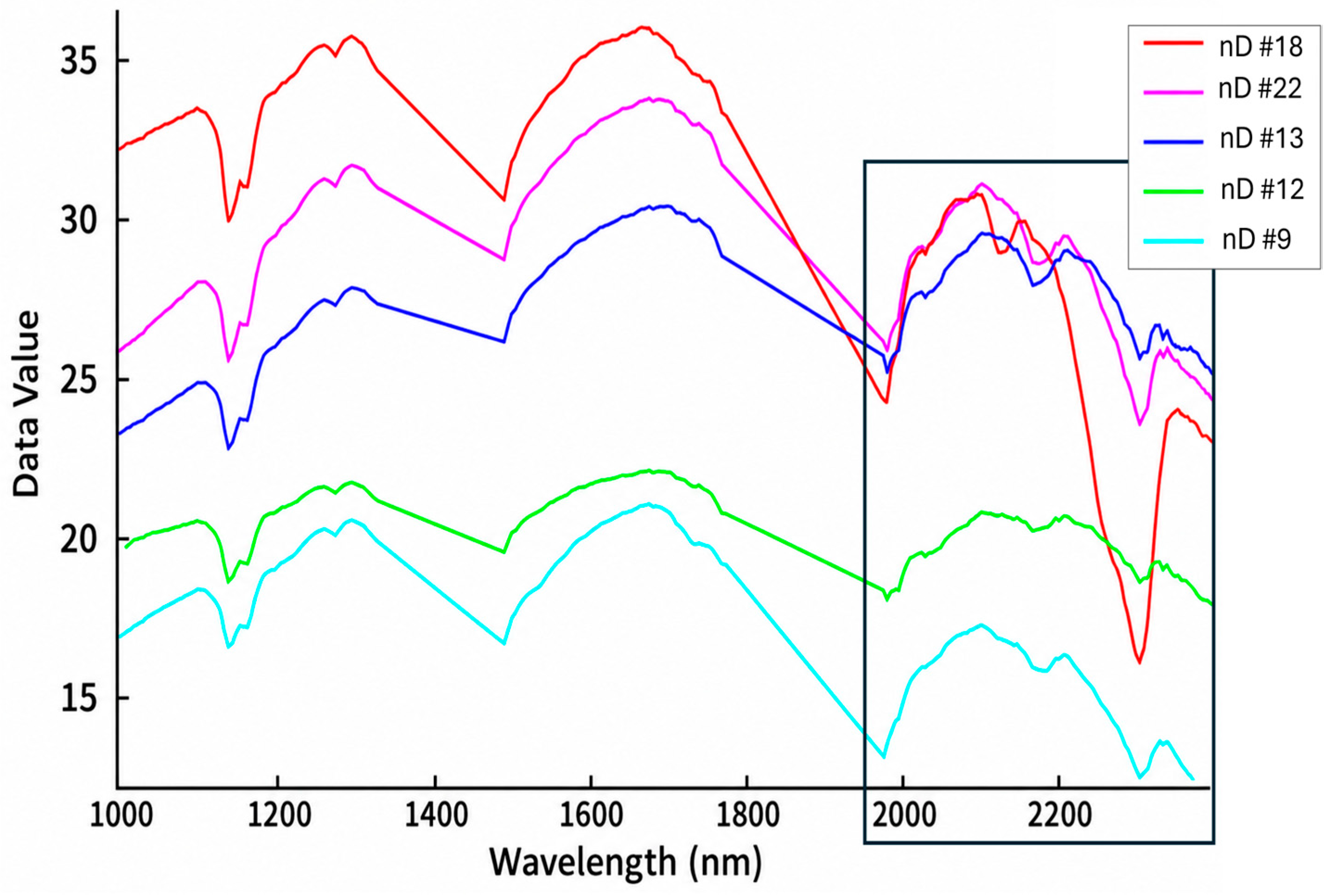
For the Pick 3 pit wall, PPI analysis initially identified 28 spectral endmembers. Of these, five dominant spectra were selected. The selection was based on two criteria applied jointly. First, spatial coverage: the five selected endmembers collectively accounted for approximately 98% of all pixels across the Pick 3 pit wall, ensuring that the reference spectra represent the dominant surface materials rather than rare or spatially isolated occurrences. The remaining 23 endmembers covered only scattered, isolated pixels with no coherent spatial distribution, frequently capturing the unmasked shadow features, and were therefore excluded as they are unlikely to represent meaningful geological units. Second, spectral distinctiveness: the five selected spectra show clearly differentiated absorption features in the 2000–2400 nm range, which is the wavelength region most diagnostic for the mineral assemblages present at this site.
Within this 2000–2400 nm range, the five endmembers exhibit the following diagnostic features (Figure 8). Two spectra (nD #9 and nD #12) show broad, progressively deepening absorption from approximately 2000 nm toward longer wavelengths, with no distinct narrow absorption band, a pattern consistent with carbonaceous or organic-rich material, which absorbs broadly rather than at specific mineral-diagnostic wavelengths. Three spectra (nD #13, nD #18, and nD #22) display distinct narrow absorption features: a prominent Al–OH absorption near 2200 nm, characteristic of clay minerals such as illite, muscovite, or kaolinite, and a carbonate absorption feature near 2330–2340 nm, characteristic of calcite and dolomite. Among these three, nD #18 shows a comparatively subdued Al–OH feature and a more pronounced carbonate absorption, while nD #13 and nD #22 show stronger Al–OH features, reflecting varying proportions of clay and carbonate phases. These differences in absorption position and depth provide sufficient spectral contrast to discriminate between the dominant surface units across the Pick 3 wall.
These five selected endmembers serve as reference spectra for the SAM algorithm. The SAM classifier then calculates the spectral angle between each pixel in the image and the reference spectra. Pixels were assigned to the class with the smallest spectral angle, corresponding to the highest spectral similarity. This technique is particularly effective for hyperspectral mineral mapping because it is insensitive to illumination differences and relies solely on spectral shape, making it well-suited for geological analysis in field conditions [45]. All SAM results were interpreted in comparison with spectra from local spectral libraries and scanned rock samples from the mine to support accurate labeling and interpretation of the classified units.

4.2.2. Deep Learning-Based Clustering (Autoencoder + K-Means)

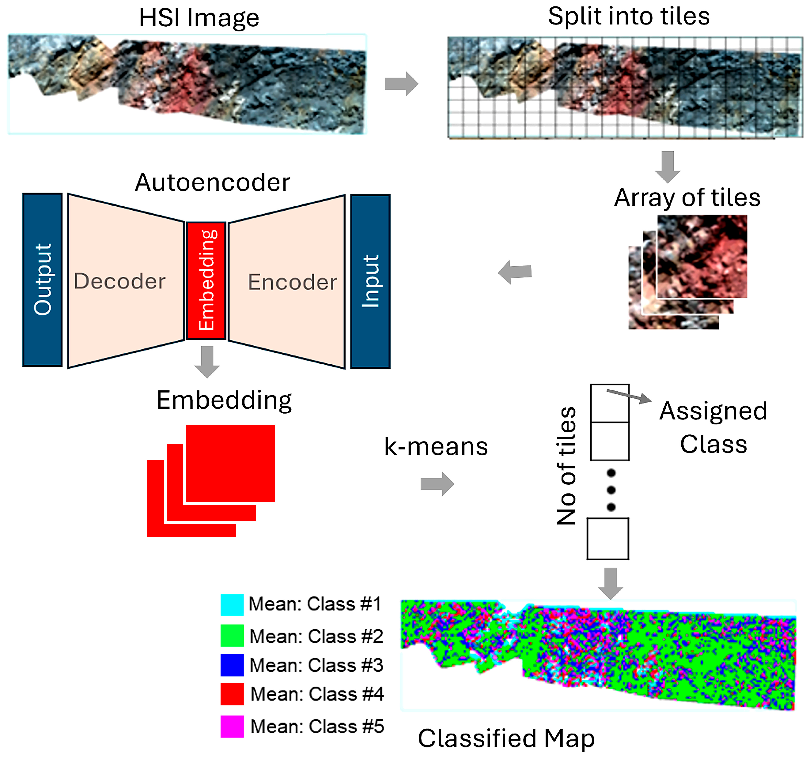
To classify hyperspectral images, we employed a deep learning-based clustering approach that combines an Autoencoder and K-means. An autoencoder is a neural network designed to learn compact representations of input data by encoding it into a low-dimensional latent space and reconstructing it at the output. Owing to their ability to capture nonlinear spectral–spatial relationships, autoencoders have been widely used for unsupervised feature extraction in hyperspectral image analysis [46,47]. Autoencoders are occasionally referred to as self-supervised because they learn through self-reconstruction [48]; however, this process does not involve external labels. In this study, the autoencoder is used for feature extraction, followed by unsupervised k-means clustering; therefore, the method is treated as unsupervised.
The overall methodology is illustrated in Figure 9 and was applied consistently to both case studies (Pick 3 and the West Wall). For each dataset, the hyperspectral image was first clipped to the region of interest. For Pick 3, oversaturated areas were removed, yielding an image of 834 × 220 pixels. For the West Wall, oversaturation was not an issue; therefore, the entire region of interest (ROI) was retained, and the image size used in this study was 1939 × 620 pixels. To evaluate the impact of spatial resolution on clustering accuracy, the image was divided into non-overlapping tiles of various sizes: 4 × 4, 8 × 8, 16 × 16, and 32 × 32 pixels. Smaller tiles captured finer spatial details but increased computational complexity, whereas larger tiles preserved broader structures at the expense of spatial precision. The autoencoder framework was then applied to these tiles. The encoder compresses each tile into a lower-dimensional latent representation (embedding), reducing redundancy while preserving key spectral features. These embeddings serve as input to K-Means clustering, which groups similar embeddings into distinct clusters. The decoder reconstructs the original tile from its compressed representation, ensuring meaningful feature extraction.
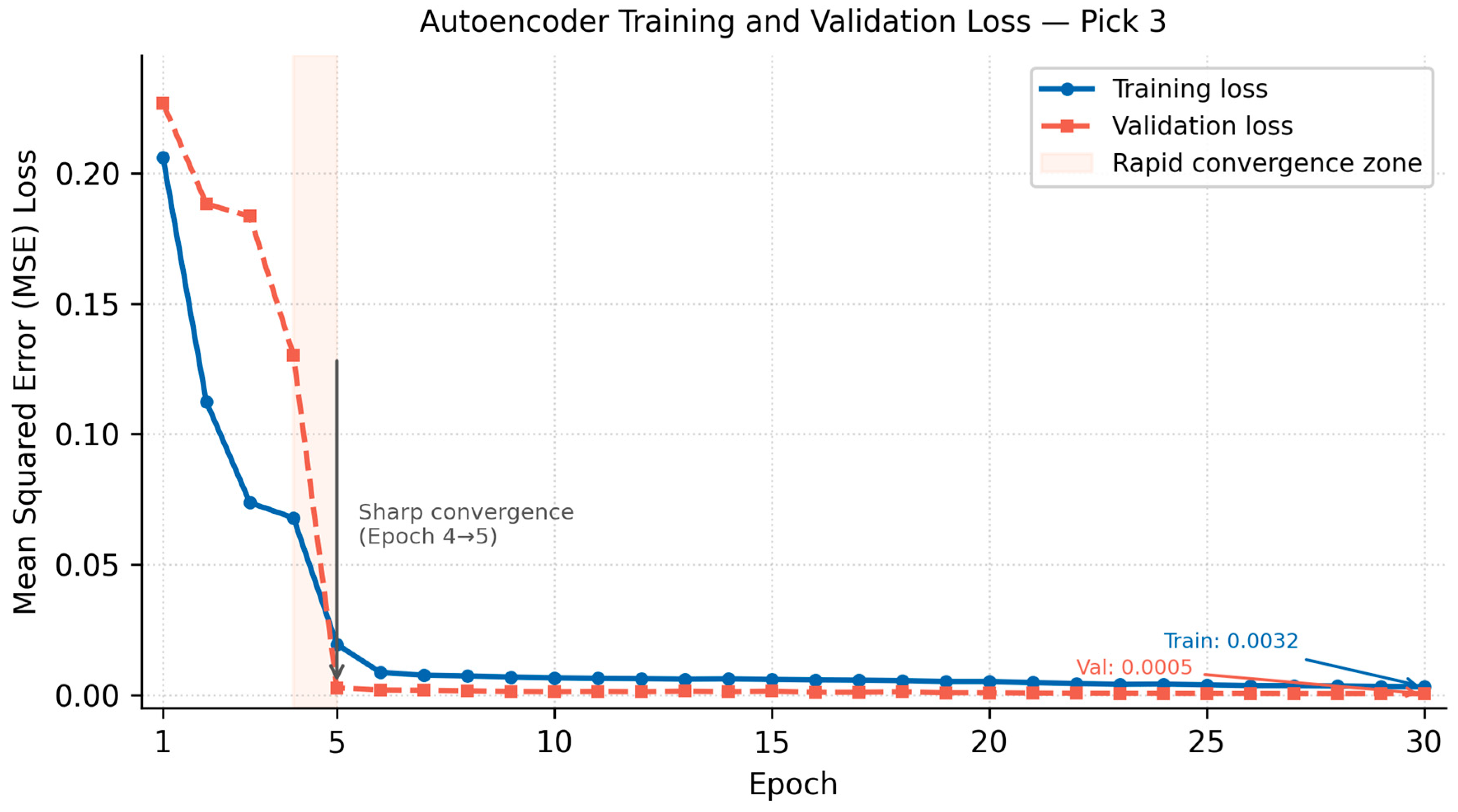
For consistency across methods, the AE model was trained using only the hyperspectral bands within the same 2000–2400 nm spectral interval employed for the SAM and BR analyses. This subset comprised 78 bands extracted from the full SWIR scene (235 bands spanning 970–2433 nm). The autoencoder follows a symmetric encoder–decoder architecture summarized in Table 3. The encoder progressively compresses each input tile through convolutional and pooling layers into a 128-dimensional latent vector; the decoder mirrors this structure using transposed convolutions to reconstruct the original input. The network was trained using the Adam optimizer with a Mean Squared Error loss function, a batch size of 256, and a maximum of 30 epochs, with early stopping based on validation loss. The training and validation loss curves are shown in Figure 10.
Both losses decreased rapidly during the first five epochs, with a pronounced convergence between Epochs 4 and 5 (training loss: 0.0679→0.0194; validation loss: 0.1303→0.0028), followed by smooth, stable convergence to final values of 0.0032 and 0.0005, respectively. The implications of this convergence pattern for classification behaviour are discussed in Section 5.3.
By applying K-means clustering to the learned embeddings, we generated a classified map of spectral clusters across the scanned pit wall. Our analysis showed that 4 × 4 pixel tiles provided the optimal balance between detail preservation and computational efficiency. For Pick 3, larger tile sizes, such as 32 × 32 (156 tiles) or 16 × 16 (676 tiles), were computationally efficient, requiring less than 2 min, but produced overly smoothed results with significant spatial variations lost due to excessive pixel merging. In contrast, smaller tiles, such as 8 × 8 (2808 tiles) or 4 × 4 (11,440 tiles), preserved much finer detail, though at higher computational cost. Although the 8 × 8 tiles captured more detail than larger configurations, they still did not fully represent the fine-scale geological variations observed in the field. The selection of the 4 × 4 configuration was based on visual comparison with the geologist’s schematic map, which is the most geologically meaningful criterion for this task, as the objective is geological unit delineation rather than reconstruction loss minimization. For Pick 3, processing the 4 × 4 tiles took approximately 5 min, while for the West Wall (75,020 tiles at 4 × 4 resolution), the processing time increased to about 23 min. Because the autoencoder assigns a single cluster label per non-overlapping tile rather than per pixel, the resulting classified maps have an effective spatial resolution equal to the tile size used (e.g., 4 × 4 pixels), coarser than the native pixel resolution of the input hyperspectral image and coarser than the pixel-level outputs of the SAM and band-ratio methods. Non-overlapping tiling was adopted to keep computation tractable given the large scene sizes involved (up to 75,020 tiles for the West Wall); pixel-level output resolution could in principle be achieved using overlapping patches or a fully convolutional architecture, at substantially higher computational cost.
Tiling was crucial because directly processing large hyperspectral images is computationally expensive. Tiling enables the model to extract spatial patterns more effectively, thereby helping the encoder learn meaningful spectral features and improving classification accuracy.

4.2.3. Band Ratio Feature Extraction

The third approach implemented in this study is feature extraction using spectral band ratios, a method designed to highlight mineralogical differences in hyperspectral imagery [49]. Band ratios are computed by dividing the reflectance values of selected spectral bands, which helps normalize illumination effects and enhance absorption features associated with specific minerals. This technique is particularly effective at enhancing spectral differences and minimizing the influence of external lighting conditions. In this study, critical spectral features were extracted by calculating targeted band ratios for each local spectrum, based on known diagnostic regions across the SWIR range. These ratios capture key variations that are often linked to mineralogical composition. The band ratios used for the classification of Pick 3 are shown in Table 4. All extracted features were compiled into a comprehensive dataset, in which each pixel in the hyperspectral image is associated with a vector of band-ratio values. This organized structure serves as input to the K-Means clustering algorithm. The algorithm groups pixels into clusters based on similarity in band-ratio features, allowing us to identify regions with similar spectral characteristics for further classification. The band ratios were derived directly from the local spectral library compiled for the Gold Bar mine by identifying absorption troughs and reflectance shoulders in each reference spectrum across the 2000–2433 nm SWIR range and constructing shoulder-to-trough ratios such that a high ratio value indicates strong absorption at a mineralogically diagnostic wavelength. The full spectral library was used, ensuring that the feature set captures the complete mineralogical range of the deposit and maximizes discriminative sensitivity in the subsequent K-means clustering step. The 28 ratios target five key wavelength regions sensitive to the dominant mineral assemblages present at Gold Bar: (1) the 2000–2136 nm continuum region, where carbonaceous material produces a broad featureless absorption distinguishable from mineral-dominated spectra; (2) the ~2160–2170 nm region, sensitive to Al–OH absorption of aluminum-rich clay minerals; (3) the ~2200–2220 nm region, corresponding to the main Al–OH absorption diagnostic of illite, muscovite, and related phyllosilicates, the dominant clay phase in the alteration system; (4) the ~2249–2300 nm region, sensitive to secondary hydroxyl mineral features; and (5) the ~2330–2350 nm region, corresponding to the CO3 absorption of calcite, dolomite, and ankerite, a key discriminator between lithological units.

4.3. Labeling and Validation

To interpret and validate the classification outputs from the three classification methods (SAM, Autoencoder with K-Means clustering, and Band Ratio-based K-Means clustering), we implemented a cross-referencing procedure using cosine similarity as a common metric for spectral comparison in remote sensing applications [50]. Cosine similarity was used to evaluate the degree of similarity between classified class mean spectra and reference spectra. Each initially unlabeled classified unit was compared against two sets of reference spectra: (1) local spectra extracted from the mine reports and (2) laboratory-acquired spectra obtained from collected rock samples. For each technique, the average spectrum of each class was computed and then systematically compared with all reference spectra within each set (local and sample) using cosine similarity. The most similar reference spectrum, based on the highest similarity score, was selected as the representative for labeling. This procedure was applied separately to the local field spectra and the lab-sample spectra, allowing us to evaluate how consistently each clustering method aligned with both field-observed and lab-condition spectral information. The labeling results are discussed further in the results section, along with visual comparisons of the classification maps and their associated spectra.
It should be noted that cosine-similarity-based comparison is used here as a common spectral matching tool for labeling and cross-checking the outputs of the three unsupervised methods, rather than as a fully method-neutral accuracy metric. In particular, because SAM uses scene-derived endmembers and is inherently based on spectral-angle matching, comparisons involving SAM may partially favor this method when interpreted purely in terms of spectral similarity. However, the reference datasets used in this study also include independent local spectral references and 17 laboratory-scanned, XRD-characterized rock samples that were external to the SAM classification process. For this reason, spectral similarity results are interpreted together with independent geological comparison, including polygon-wise agreement with the mine geologist’s schematic map.

5. Results and Discussion

This section is divided into two parts corresponding to the two scanned pit walls: Pick 3 and West Wall. Each subsection presents the classification results obtained from the three unsupervised techniques described above, followed by spectral analysis, similarity assessments, and comparisons with the mine geologist’s geological map of the walls.

5.1. Pick 3 Pit Wall

5.1.1. Classification Results from the Three Techniques

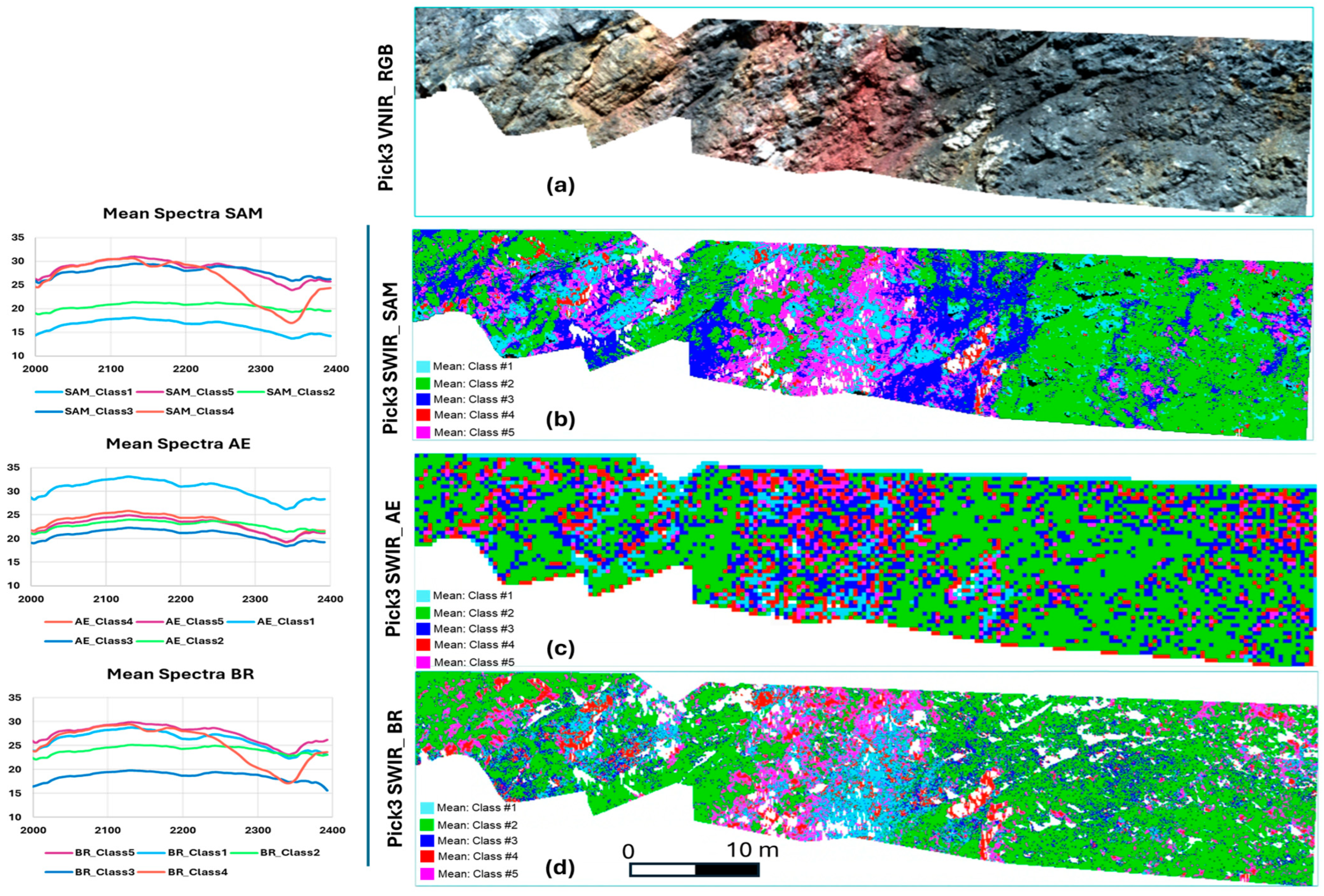
For the Pick 3 wall, three classification maps were generated using SAM, AE, and BR. These maps are initially unlabeled, representing purely data-driven spectral groupings. Alongside each classified map, the mean spectrum of each class is shown in Figure 11 to visually evaluate intra-class spectral consistency and inter-class separability.

5.1.2. Similarity Analysis with Reference Spectra

To assign geological meaning to the classified units, we computed the cosine similarity between the mean spectrum of each class and the two reference datasets mentioned earlier. For each class and technique, the most similar spectrum from each reference set was identified. These matches form the basis for labeling and provide insight into which spectral references each technique aligns with most closely. The results are summarized in Table 5.
A key observation is the strong agreement between the SAM and BR techniques, both in terms of alignment with the most similar rock samples and their corresponding local spectra. In general, most classes show consistent similarity patterns between these two methods, whereas AE produced different results, with many mean spectra labeled as illite-calcite. Among the SAM and BR outputs, Class 4 provides a clear example of this strong agreement, closely matching the Hematite–quartz–calcite spectrum in the local spectral reference set. This similarity is further confirmed by the rock sample GB1-1 (Grey Bartine waste with weak hematite joint stains), which exhibits comparable spectral characteristics. This consistent match between local spectral features and physical rock samples strengthens the validity of the classification and supports the interpretation that Class 4 likely represents hematite-bearing altered waste material. It should be noted that quartz is not directly detected from the SWIR hyperspectral data used in this study, as quartz does not exhibit diagnostic absorption features within the investigated wavelength range. The identification of quartz in the analyzed samples is therefore based on the supporting mineralogical evidence obtained from XRD analysis (Table 2).
In contrast, the AE-based clustering shows a different pattern. While it identifies several of the same rock samples (e.g., GB3-4 and GB3-5) as most similar, it associates Class 4 with GB3-1 as the closest rock sample. The most similar local spectrum for this class is illite–calcite rather than hematite–quartz–calcite, as observed in the SAM and BR results. Furthermore, in the AE output, the illite–calcite spectrum appears as the most similar reference for four out of the five classes (Classes 1, 3, 4, and 5). This suggests that the latent features learned by the autoencoder emphasize broader spectral similarities, potentially reducing sensitivity to subtle mineralogical variations captured by SAM and BR.
To quantify these qualitative observations, we compared the best-match class labels assigned by each technique across both reference sets (Table 5 and Table 6).
We additionally examined the separation margin, the difference between each class’s best-match similarity score and its second-best alternative, as a secondary measure of classification decisiveness (Table 7). Against the local spectral library, SAM and BR achieved a mean margin of 0.00079, roughly twice that of AE (0.00036), and AE resolved only two distinct reference labels across its five classes (versus three for SAM and BR), consistent with AE’s tendency toward less distinct class separation. Against the lab rock samples, margins were smaller and comparable across all three techniques (0.00014–0.00016), which we attribute to the more continuous, mixed mineralogy among individual rock specimens (Table 2) relative to the more discrete categories in the local spectral library. We also tested the raw mean cosine similarity score as a candidate discriminating metric and found it did not differ meaningfully between techniques (all > 0.996, differences < 0.001; Table 7), confirming that the absolute similarity score is a weak discriminator in this context.
Following the analysis of similarity scores and separation margins (Table 6 and Table 7), we further quantified the consistency of class assignments by comparing the best-match class labels assigned by each technique across both reference sets (Table 8). SAM and BR assigned identical class labels in all 10 comparisons (100%), comprising 5 rock sample comparisons and 5 local spectra comparisons. In contrast, SAM and AE, and BR and AE, each agreed in only 6 of the 10 comparisons (60%). The two points of disagreement for AE were Class 3, where SAM and BR identified a carbonaceous affinity that AE instead associated with an illite-calcite reference, and Class 4, where SAM and BR consistently matched a hematite–quartz–calcite assemblage (local spectra) and rock sample GB1-1 (lab sample), while AE matched an illite-calcite reference and sample GB3-1, respectively. This quantitative comparison confirms the close correspondence between SAM and BR and identifies Classes 3 and 4 as the specific units where the autoencoder’s learned representation diverges from the other two techniques.
The XRD compositions of the best-matching rock samples (Table 2) provide independent mineralogical support for the spectral class labels. For Classes 1 and 5, assigned an Illite-Calcite label across all three techniques, the best-matching sample GB3-4 (59.2% calcite, 3.4% muscovite as the dominant phyllosilicate) is consistent with a carbonate-clay assemblage; the illite interpretation is supported by the SWIR spectral signature, as illite and muscovite are chemically related dioctahedral micas not always fully resolved by XRD at low concentrations. For Class 4, assigned a Hematite–Quartz–Calcite label by both SAM and BR, the best-matching sample GB1-1 (63.9% calcite, 10.8% quartz) confirms the carbonate and silica components; the hematite component is absent in the XRD results due to its fine-grained, poorly crystalline nature at these concentrations, but is independently confirmed by the VNIR-derived iron oxide map. For Classes 2 and 3, assigned a Carbonaceous label by SAM and BR, the best-matching sample GB3-5 shows elevated amorphous content (14.4%), consistent with poorly crystalline carbonaceous material that is spectrally active in the SWIR but not separately quantified by XRD. For AE Class 4, matched instead to GB3-1 (60.5% calcite, 13.3% dolomite) and labeled Illite-Calcite rather than Hematite–Quartz–Calcite, the XRD composition lacks the quartz enrichment and iron-oxide signature characteristic of GB1-1, highlighting how the spatial-spectral integration of the model smooths out discrete, localized anomalies, leading to an interpretation that favors the dominant background matrix over high-contrast target signatures.
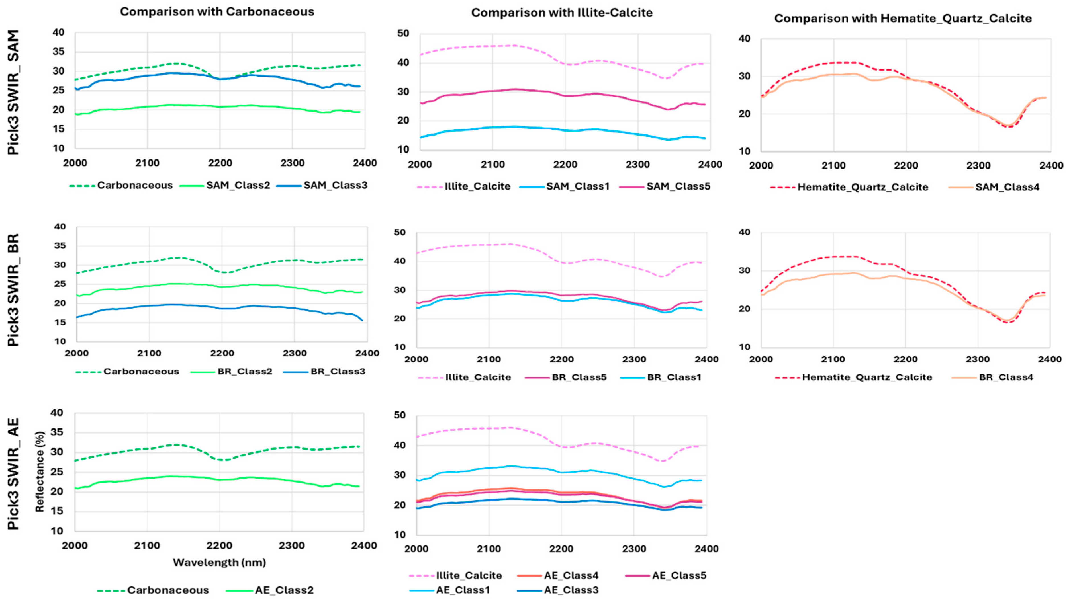
Figure 12 illustrates the comparison between the mean spectra of the classified classes derived from each technique and the local reference spectra, highlighting spectral trends and their mineralogical relevance. In the case of the SAM, several classes exhibit excellent agreement with specific local reference spectra. Notably, Class 4 (shown in red) aligns almost perfectly with the red-dotted local spectrum, which corresponds to a Hematite–Quartz–Calcite assemblage. Similarly, Class 2 (green) and Class 3 (blue) align well with the green-dotted local spectrum, associated with carbonaceous material. In addition, Class 5 (purple) and Class 1 (light blue) in SAM follow the spectral trend of the pink-dotted local spectrum, which is linked to an Illite–Calcite composition. These clear matches indicate that SAM maintains strong sensitivity to mineralogical distinctions and preserves spectral shape features critical for class differentiation.
The AE results show that Class 2 (green) also aligns well with the carbonaceous spectrum, consistent with results from the other techniques. However, the remaining AE classes (Classes 1, 3, 4, and 5) have very similar spectral shapes, differing mainly in overall intensity rather than in distinct spectral features. These trends align most closely with the pink-dotted spectrum from the local library, representing illite–calcite. This clustering around a single spectral trend suggests that the AE method may have generalized some of the finer distinctions between mineral groups, likely due to dimensionality reduction, the nature of reconstruction-based learning, and the effect of tile size, where larger tiles can average out subtle spectral variations. The BR technique shows many of the trends observed in SAM. This consistency underscores that BR and SAM both retain geologically meaningful spectral features, enabling clear distinctions among units dominated by hematite, carbonaceous material, or illite-bearing lithologies. The presence of a residual ~2200 nm feature within the carbonaceous classes likely reflects intimate mixing of carbonaceous matter with illite-bearing clay alteration rather than a spectral property of carbon itself; pure carbonaceous material produces only a broad, featureless absorption in the 2000–2136 nm continuum (Section 4.2.3), whereas the 2200 nm feature is diagnostic of the Al–OH absorption in illite/muscovite.
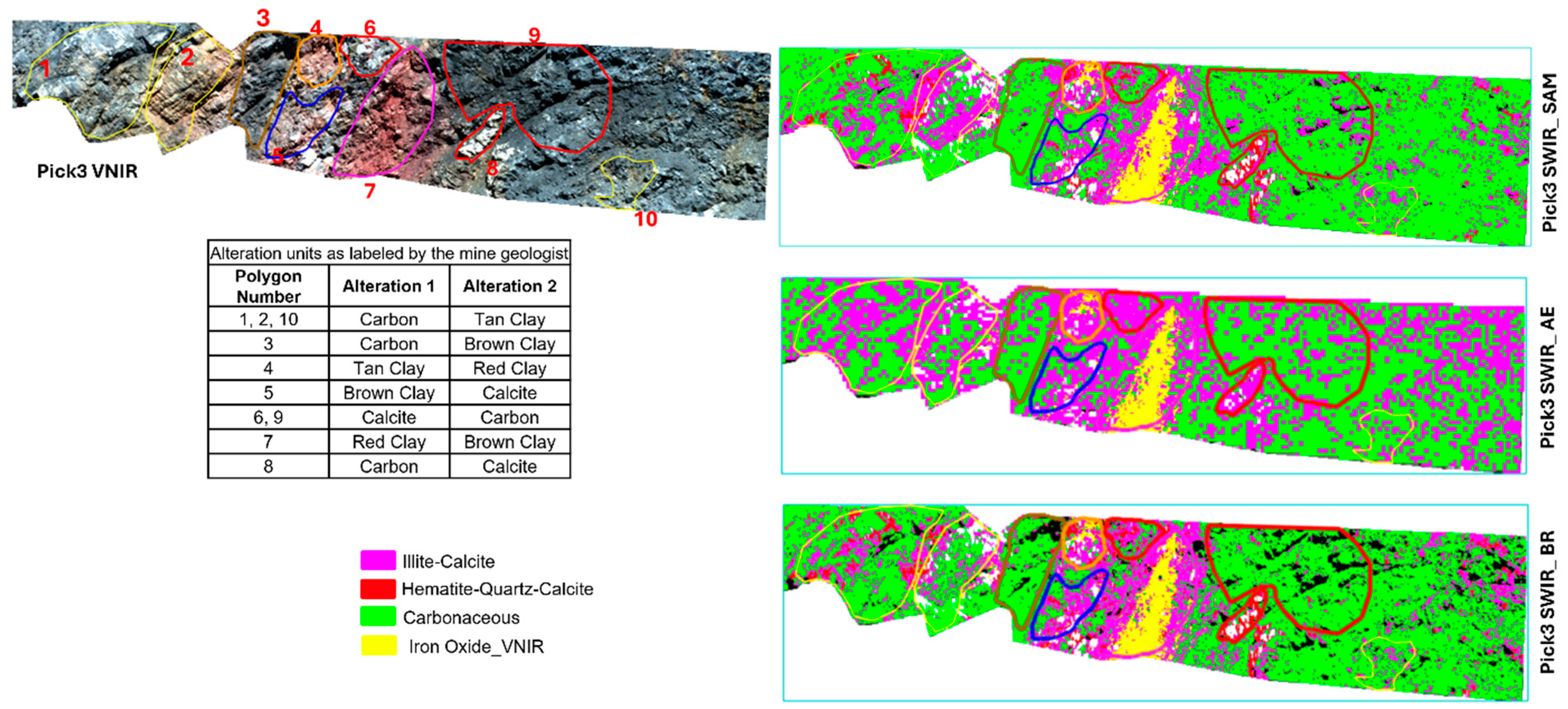
In addition to the spectral classification results from the SWIR region, an iron oxide distribution map of the Pick 3 wall was generated using the SAM technique applied to the VNIR image. This classification used reference spectra for hematite obtained from the USGS standard spectral library, targeting ferric iron absorption features characteristic of iron oxide minerals. For this VNIR-based iron oxide mapping, a maximum SAM angular threshold of 0.1 radians was strictly applied, with any pixels exceeding this threshold classified as unmapped. The iron oxide map was then overlaid on the SWIR-based classified images generated by SAM, AE, and BR, each of which had been labeled using cosine similarity with local reference spectra. As shown in Figure 13, the Pick 3 wall classification results obtained using SAM, AE, and BR are presented alongside the VNIR-derived iron oxide map and the schematic geological interpretation provided by the mine geologist. The geologist’s map divides the wall into ten polygons representing the dominant field-observed materials or alteration styles, expressed as mixed labels such as Carbon/Tan, Brown/Calcite, and Red/Brown. These polygons provide an independent field-based reference for evaluating whether the spectral classes derived from hyperspectral data correspond to the major geological domains exposed on the wall.
Comparison of the SWIR-based classification maps with the geologist’s polygons and the VNIR iron oxide map shows that all three techniques captured the principal material domains of the Pick 3 wall, but with different levels of mineralogical specificity. Across the three methods, polygons containing a carbonaceous component were generally mapped as Carbonaceous in the SWIR classifications, particularly in Polygons 1, 3, 9, and 10, where carbon-bearing units were consistently identified by all techniques. In contrast, polygons associated with calcite- and tan clay–rich materials were typically represented by the Illite–Calcite class, particularly in Polygons 4, 5, and 6. These relationships indicate that the SWIR classifications successfully captured the major contrast between carbon-rich and clay–carbonate domains in the Pick 3 wall.
To provide a quantitative basis for this comparison, a polygon-wise agreement analysis was performed using the ten geologist-defined polygons (Table 9). For each polygon and each classification technique, the dominant spectral class was identified as the class containing the highest proportion of pixels within that polygon. Agreement was then evaluated using a simplified spectral-to-geological correspondence in which Carbonaceous was considered consistent with polygons containing a carbonaceous component, Illite–Calcite with calcite- and tan clay-dominated polygons, and Hematite–Quartz–Calcite with red clay/iron-rich alteration. Because several geologist polygons represent mixed field interpretations rather than single lithological units, and because brown clay does not correspond uniquely to a single SWIR spectral class, brown-clay labels were treated as non-diagnostic in the agreement assessment rather than being forced into one mineralogical category. Using this polygon-wise dominant-class comparison, SAM and AE showed agreement or partial agreement in 9 of the 10 polygons (90%), whereas BR showed agreement in 8 of the 10 polygons (80%).
Although AE achieved the same polygon-level match count as SAM, the polygon-wise results and class distributions show that the three methods do not perform equivalently in terms of geological discrimination. AE produced broader class assignments dominated by Carbonaceous and Illite–Calcite, which increased polygon-level correspondence in mixed units but reduced the ability to separate internal mineralogical variability. This is also reflected in the mean dominant-class proportion per polygon, which was 73.4% for AE, compared with 66.5% for SAM and 66.9% for BR. The higher AE value therefore reflects stronger within-polygon class concentration rather than necessarily greater geological precision. In contrast, SAM and BR preserved greater mineralogical variability, particularly through the presence of Hematite–Quartz–Calcite and more heterogeneous mixtures of Carbonaceous and Illite–Calcite classes within clay–carbonate polygons. This makes SAM and BR more informative for interpreting fine-scale alteration patterns and internal lithological heterogeneity.
A particularly important example is Polygon 7, which the geologist mapped as Red/Brown clay. In the SWIR classifications, this polygon is dominated by Illite–Calcite in all three methods, so none of the SWIR maps alone identifies Hematite–Quartz–Calcite as the dominant class in this zone. However, the VNIR-derived iron oxide map shows a strong concentration of iron-oxide-bearing pixels in Polygon 7, confirming that this area is associated with hematitic alteration. This demonstrates that the mineralogical character of the red/brown clay zone is best resolved by integrating VNIR and SWIR information, with the VNIR data providing sensitivity to iron oxides and the SWIR data capturing the associated clay–carbonate assemblages. In this sense, the discrepancy between the SWIR-dominant class and the geologist’s red/brown interpretation does not indicate failure of the hyperspectral workflow but rather highlights the complementary roles of the VNIR and SWIR spectral ranges.
Overall, the combined visual, spectral, and polygon-wise comparisons indicate that all three methods captured the major geological domains of the Pick 3 wall, but with different strengths. AE yielded high polygon-level agreement because its broader classes correspond well to mixed geologist polygons, whereas SAM and BR retained greater mineralogical specificity by distinguishing carbonaceous, clay–carbonate, and hematite-bearing materials more explicitly. When interpreted together with the VNIR iron oxide map, SAM and BR provide the most geologically informative representation of pit-wall alteration variability, while AE offers a more generalized but spatially coherent classification of the dominant wall materials. These results demonstrate the value of integrating VNIR and SWIR hyperspectral information with the geologist’s observations to improve the reliability and interpretability of pit-wall geological mapping.

5.2. West Wall

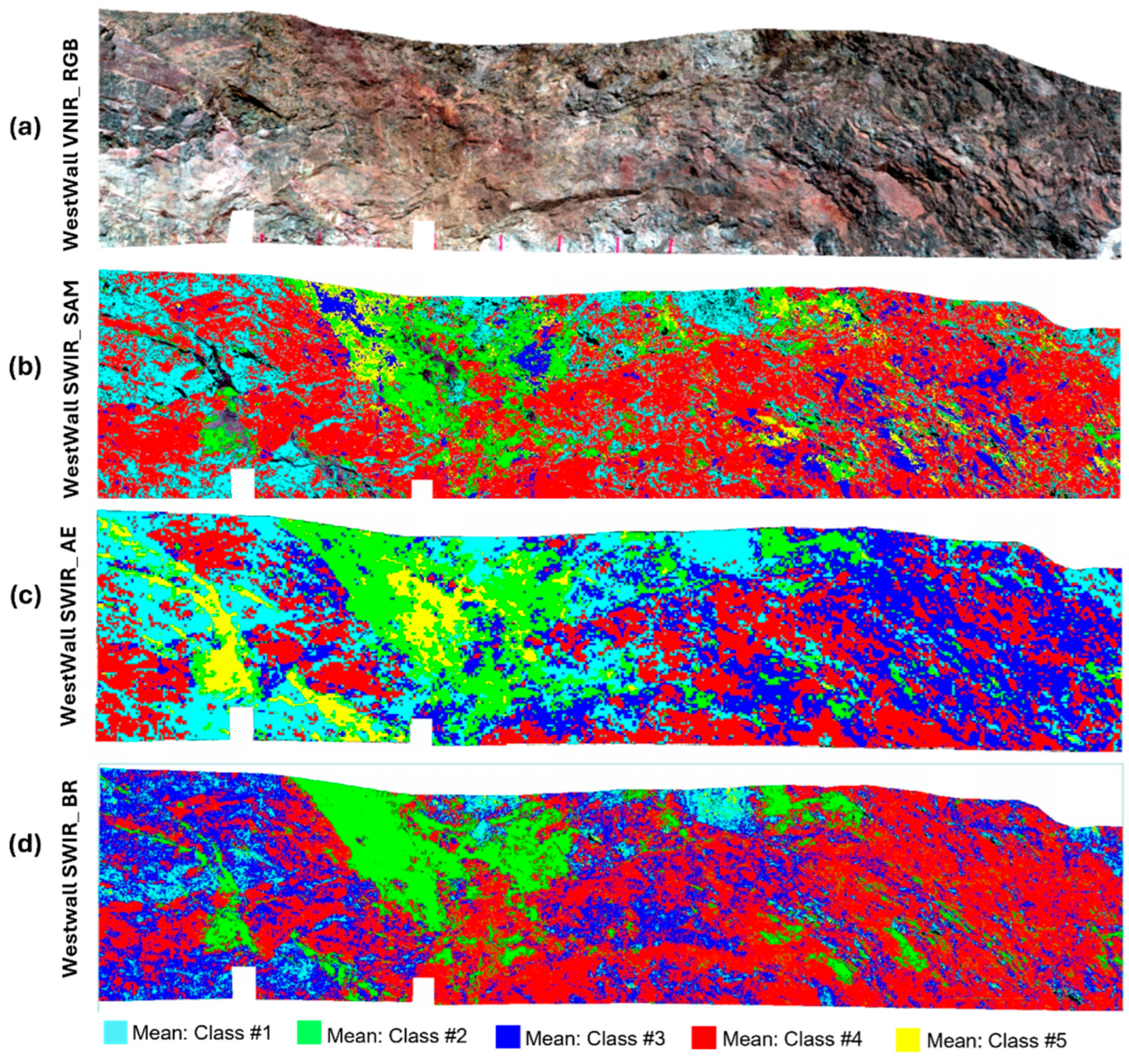
The same analysis steps used for the Pick 3 pit wall were applied to the West Wall dataset. Unlabeled maps from SAM, AE, and BR for the West Pit wall are shown in Figure 14.
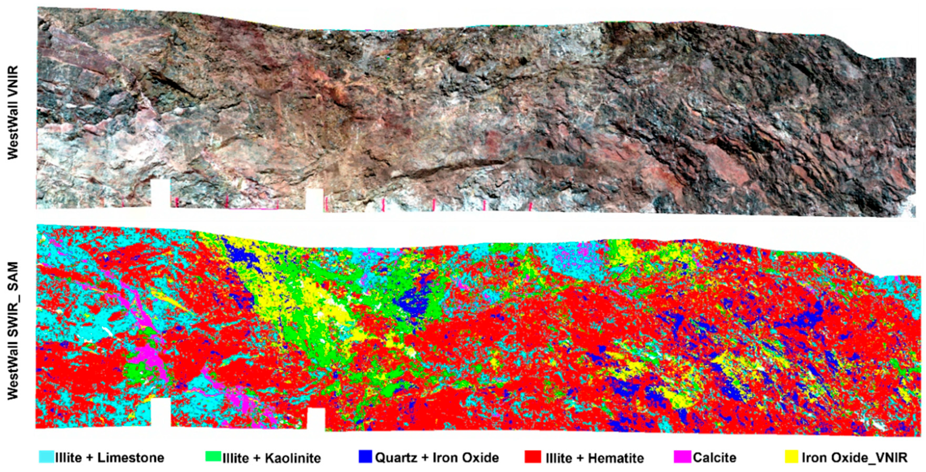
Unlike Pick 3, where rock samples and local spectral references supported class labeling, the West Wall lacked direct validation sources, as the available rock samples and local spectral references were collected in proximity to the Pick 3 wall and represent different geological conditions from those of the West Wall. Accordingly, all classification results for the West Wall should be interpreted as geologically informed qualitative assessments rather than quantitatively validated outputs, and no direct performance comparison is drawn between the two walls. Therefore, the interpretation and labeling of the classification outputs from SAM, AE, and BR were based primarily on the geologist’s expertise and structural interpretation. Despite this limitation, the combined use of the hyperspectral techniques provided a detailed view of the wall’s mineralogical and structural variability. Among the three methods, SAM proved particularly effective in identifying zones with complex alteration patterns, especially within high-clay fault zones, while AE and BR showed reduced sensitivity to fine-scale spectral variability in faulted areas but successfully delineated the boundaries between major alteration domains. Figure 15 presents the labeled SAM map based on the mine geologist’s observations. Similar to the approach used for Pick 3, an iron oxide distribution map of the West pit wall was generated using the SAM technique applied to the VNIR image. This iron oxide map was then overlaid on the SWIR classification results from the SAM method.
According to the mine geologist, the hyperspectral outputs for the West Wall identified several fault-controlled features characteristic of Carlin-style gold deposits. In these systems, mineralizing fluids migrate along fault conduits and fracture networks, promoting extensive alteration and ore deposition. The hyperspectral scans revealed abrupt alteration boundaries that likely correspond to structural pathways, features that might not be easily detectable using traditional scanning or mapping methods such as LiDAR, which can be restricted by limited visibility or scanning angles. A key observation from the West Wall interpretation was the distribution of calcite-bearing zones. Identifying calcite is essential to understanding fluid evolution within Carlin-type systems.

5.3. Comparative Evaluation and Interpretation

A comparative analysis of the classification results from the Pick 3 and West pit walls highlights the strengths and limitations of the three techniques, SAM, AE, and BR, with respect to spectral discrimination, spatial coherence, and alignment with reference data. In the Pick 3 pit wall, the geology is relatively simple and the alteration zones are more distinct, allowing SAM and BR to clearly capture significant spectral differences, particularly those related to hematite and carbonaceous materials. These two techniques preserved fine spectral details and diagnostic absorption features, resulting in strong agreement with both the local reference spectra and the spectra of the scanned rock sample. Their outputs also aligned well with geologist-labeled units and the VNIR-derived iron oxide distribution, providing high confidence in their ability to delineate lithological boundaries.
In contrast, interpretation of the West pit wall relied primarily on the mine geologist’s observations because direct validation data were unavailable. In this structurally complex setting, SAM was particularly effective at identifying alteration patterns within high-clay fault zones; its endmembers were derived independently via a fresh PPI extraction on the West Wall’s own scene, allowing it to capture that wall’s specific spectral diversity. BR, by contrast, applied the same 28 band ratios derived from the Pick 3 local spectral library (Table 4), without recalibration to the West Wall. We consider this less problematic than a like-for-like reuse of calibration might suggest, since these ratios target wavelength positions corresponding to Al–OH and CO3 absorption features that are mineralogically generic to clay and carbonate phases across Carlin-type alteration systems, rather than calibrated to Pick 3’s specific spectral idiosyncrasies; however, no local spectral library was available for the West Wall to directly confirm this assumption, and we treat BR’s reduced sensitivity there as a limitation of this specific application rather than a validated finding. AE, retrained independently on West Wall tiles, showed a distinct form of reduced sensitivity to fine-scale spectral variability, discussed below, arising from its tile-based spatial compression rather than from any reference-spectrum limitation. Despite these differences in cause, both BR and AE successfully delineated the boundaries between major alteration domains. This contrast between the two pit walls highlights an important methodological observation: SAM and BR produced closely consistent, geologically reliable classifications across both walls, with SAM showing the strongest correspondence to reference spectra and confirmed mineral assemblages, particularly in resolving subtle spectral variations and mineralogical boundaries at a fine spatial scale owing to its pixel-based implementation. AE achieved comparable polygon-level agreement to SAM at Pick 3 but with reduced mineralogical specificity, tending toward broader, more generalized class groupings.
It is also useful to distinguish the classification behaviour of the three methods. Both SAM and BR assign each pixel directly to a single class, whereas AE first compresses each 4 × 4 tile into a latent representation before clustering, which could, in principle, better capture mixed or transitional spectra. However, because AE uses non-overlapping tiles, fine-scale spatial variability is averaged before classification. As a result, SAM’s stronger performance in the fault-controlled zones is mainly due to its preservation of full pixel-level spatial detail, rather than to any advantage of hard class assignment itself.
Their performance was satisfactory in simpler geological settings, such as the Pick 3 wall, where alteration zones were relatively homogeneous, but their ability to resolve overlapping or mixed spectral signatures decreased in the more complex geological environment of the West wall. For the AE in particular, a key factor influencing this behaviour is the tile-based input configuration, in which the hyperspectral cube was divided into non-overlapping 4 × 4 pixel tiles prior to training. While this approach reduced computational demands and stabilized model convergence, it also smoothed local spectral variability and reduced spatial continuity across structural boundaries.
It is important to note that although the autoencoder is used here as a classification approach by combining it with K-means clustering, its learning objective differs fundamentally from those of SAM and Band Ratio, and also from the supervised or semi-supervised deep learning architectures that typically demonstrate superior performance in the hyperspectral classification literature. In those studies, deep learning models are trained with class-labeled data and classification-oriented loss functions that explicitly reward mineralogical discrimination. In contrast, the autoencoder used here is trained in a fully unsupervised manner, minimizing MSE reconstruction error without any mineralogical supervision signal. Under this objective, the learned latent features reflect spectral variance structure rather than diagnostic absorption differences, which explains why the AE results showed broader spectral groupings than SAM and BR.
Several factors explain why the autoencoder (AE) tended to generalize these mineral classes. First, compressing each 4 × 4 × 78 patch (1248 values) into a 128-dimensional latent vector results in a compression ratio of roughly 9.8:1. This aggressive compression forces the network to prioritize broad, high-variance spectral features, namely the widespread carbonate-clay signature, while discarding the subtle, diagnostic absorption features that SAM and BR explicitly target. Second, the training loss curves (Figure 10) show that both training and validation losses decreased steadily across all 30 epochs, with final values of 0.0032 and 0.0005, respectively, confirming stable model convergence. The pronounced loss reduction observed between Epochs 4 and 5 reflects the spectral homogeneity of the Pick 3 dataset, where the dominant carbonate-clay spectral trend shared across multiple mineralogical units represents a relatively simple variance structure for the encoder to capture, rather than any pathological training behaviour. Third, dividing the hyperspectral cube into non-overlapping 4 × 4 pixel tiles artificially smoothed local spectral variations and disrupted spatial continuity at geological boundaries. The block-like artifacts visible in the AE classification maps stem directly from this tiling strategy rather than an inherent flaw in the autoencoder approach itself. It is important to clarify the scope of this spatial–spectral approach. In this study, the autoencoder was trained and applied separately for each pit wall (Pick 3 and West Wall), and no attempt was made to transfer the model between scenes or deposits. This distinction is relevant because the Gold Bar pit walls contain fine-scale and spatially variable alteration, meaning that a model trained on fixed 4 × 4 tiles may learn not only mineralogical patterns but also local textural or structural features specific to that wall. In contrast, spectral signatures are more directly related to mineral composition and are therefore expected to be more consistent between pit walls of the same deposit type than with local spatial arrangements. For this reason, the tile-based spatial–spectral design used here is appropriate for within-scene classification, but a purely spectral pixel-based model, or a more generalized representation of spatial context, may be more suitable if the goal is to apply a single trained model across multiple scenes without retraining. This is noted as a consideration for future work rather than a limitation of the present study.
These observations highlight that AE’s generalization behavior in compositionally overlapping systems is a consequence of its reconstruction-based learning objective and compression architecture rather than a fundamental limitation of the method. Future implementations could address this through increased latent space dimensionality, incorporation of spectral-discriminative components into the loss function, or overlapping tile configurations to reduce boundary artifacts. While the current implementation effectively maps broader alteration domains, a useful capability for coarse-scale structural delineation, these modifications represent productive directions for improving mineralogical precision in future hyperspectral mapping workflows.
It should be noted that a key limitation of the Pick 3 comparative analysis is the size of the validation dataset, which consists of 17 rock samples and 15 local reference spectra. While these data capture the full mineralogical range of the Gold Bar deposit, corroborated by independent XRD analysis and site-wide reporting, and successfully identify the dominant alteration assemblages, the limited sample size lowers the statistical robustness of the per-class cosine similarity metrics. Consequently, the separation margins and label-agreement statistics in Table 6, Table 7 and Table 8 should be interpreted as a measure of how the three classification methods perform relative to one another within this specific framework, rather than as a definitive, independent ground-truth validation. This constraint is typical of operational mine-site hyperspectral studies, where active production schedules, strict safety protocols, and restricted wall access prevent systematic, comprehensive sampling. Expanded reference datasets, including samples collected directly from the mapped pit wall surfaces under controlled conditions, would strengthen future studies of this kind.
Based on the comparative results across the two pit walls, the following practical guidance is offered for method selection in operational hyperspectral pit-wall mapping workflows. SAM is recommended as the primary classification method when a site-specific spectral library or reference spectra from chip trays, core samples, or laboratory scanning are available, as its reference-based design directly exploits mineralogical prior knowledge and consistently produces the most precise alteration discrimination across both simple and complex geological settings in this study. BR provides a reliable and computationally efficient alternative when diagnostic absorption wavelengths for the target mineral assemblages are known and a spectral library is available for ratio design; its performance at Pick 3 was closely comparable to SAM, and it requires no endmember extraction step, making it preferable in settings where PPI analysis is impractical. AE is most appropriate when no reference spectra are available, and the mapping objective is broad alteration domain delineation rather than precise mineral identification, for example, as a first-pass screening tool in early-stage exploration or in structurally complex settings where reference-based methods cannot be reliably anchored. In settings where iron oxide distribution is a key mapping objective, integrating VNIR-derived iron oxide mapping with SWIR classification is essential, as demonstrated by the Pick 3 results, where SWIR-based classification alone did not reliably identify hematite-bearing zones subsequently confirmed by the VNIR iron oxide map. Where resources allow, running all three methods in parallel and using SAM-BR agreement as a confidence indicator and AE divergence as a flag for geologically ambiguous zones offers the most comprehensive basis for geological interpretation, as demonstrated by the quantitative agreement analysis in Table 6, Table 7 and Table 8.
The three classification techniques also differ in their sensitivity to illumination variability, pit wall roughness, and shadow effects inherent to open-pit scanning environments. To minimize these effects, empirical line correction was applied to all hyperspectral data during preprocessing to normalize reflectance across the scene, and scanning times were selected to reduce directional illumination variability: the Pick 3 wall was scanned at 3:00 PM and the West Wall at noon (12:00 PM) to achieve more uniform solar illumination geometry. Additionally, image sections with significant shadow coverage were excluded from analysis where possible. Despite these measures, residual illumination variability and localized shadows from wall relief remain present in both datasets, and their effects on each classification technique differ. SAM is theoretically robust to multiplicative illumination changes, as spectral angle is invariant to uniform reflectance scaling, but remains sensitive to residual additive illumination effects and surface-normal variation caused by wall roughness, which alter spectral shape rather than amplitude. BR similarly benefits from the normalizing effect of ratioing, which cancels multiplicative illumination differences between bands, but is susceptible to noise when roughness-induced shadowing affects numerator and denominator bands unequally. AE is the most sensitive of the three methods to residual illumination variability, as its reconstruction-based training objective operates on absolute reflectance values; tiles acquired under slightly different illumination conditions present inconsistent input distributions that the encoder must either generalize over, potentially at the cost of spectral discrimination, or separate into illumination-driven rather than mineralogically meaningful clusters. This sensitivity may have contributed to the broader spectral groupings observed in AE results, where tiles with suppressed spectral contrast due to residual shadowing or oblique illumination would spectrally resemble the dominant carbonate-clay trend and be absorbed into that cluster.
At the Gold Bar mine, specifically within the West Wall, the geologist observed calcite pods and veins both above and within potential ore zones. Although calcite itself does not host gold due to the absence of binding elements, it frequently occurs alongside gold-bearing clay minerals, which infiltrate through fractures and cleavage planes in calcite. This association suggests a genetic link between calcite precipitation and gold-bearing fluid pathways. Therefore, integrating hyperspectral data with geological interpretation enhances understanding of both structural controls and alteration zonation, providing a valuable framework for refining exploration models and targeting mineralization in Carlin-style systems where direct ground validation is unavailable.
Compared with previous work using UAV-mounted RGB imaging and unsupervised learning, the hyperspectral approach presented in this study represents a substantial advance in geological mapping. While RGB imaging is accessible and effective for geological interpretation, it is limited to the visible light range and lacks the spectral resolution required for accurate mineral identification. In contrast, hyperspectral imaging captures detailed spectral data across a broader range, including the SWIR region, enabling detection of subtle compositional variations and alteration features invisible to RGB sensors. This enhanced capability yields more precise and comprehensive geological information. For example, in the Pick 3 wall case study, hyperspectral imaging enabled the accurate detection of carbonaceous zones associated with preg-robbing during gold leaching, thereby inhibiting gold recovery due to naturally occurring carbonaceous matter [51]. By identifying and delineating these zones, mine planners can proactively adjust extraction strategies to selectively stockpile this problematic carbonaceous ore. Similarly, detecting clay-rich zones provides critical input for mine operations, as clays affect ore handling, grinding performance, and recovery efficiency. This information enables planners to adjust blasting and ore blending strategies to mitigate processing challenges. Beyond processing, hyperspectral classification maps can highlight mineralogical zones associated with varying rock strength, providing useful input for pit wall stability assessment and short-term mine planning. On the West wall, hyperspectral scanning revealed a fault zone marked by high-clay alteration that was not evident in the LiDAR-derived structural mapping. This highlights the complementary strengths of the two methods: while LiDAR effectively captures geometric and planar features, hyperspectral imaging detects mineralogical and alteration signatures that may not be visible in structural datasets. Integrating these mineralogical insights with LiDAR-based structural data enhances the reliability of mine-scale geotechnical and geological models, supporting more informed stability assessments and operational decision-making in active pit environments. Future work combining both technologies would likely improve the correction of geometric distortions in hyperspectral data and provide a more complete understanding of pit-wall conditions.
Compared with traditional pit wall mapping by mine geologists in the field, hyperspectral imaging offers clear advantages in efficiency and safety. Manual mapping requires direct access to pit walls, which is time-consuming and labor-intensive, and can expose geologists to hazardous conditions such as rockfalls or unstable slopes. In contrast, hyperspectral mapping can be conducted from a safe distance, reducing field exposure while still capturing high-resolution mineralogical detail. Although hyperspectral analysis provides quantitative, objective data on mineralogy, including subtle variations in clay and carbonaceous content that may be difficult to identify visually, it should be viewed as a complementary tool rather than a replacement for geological expertise. System setup, calibration, and interpretation still rely on geological knowledge, much as XRD analysis requires expert input to relate elemental or diffraction data to specific minerals. From a time perspective, while field mapping may take several hours to cover a wall, the hyperspectral workflow (including data acquisition, preprocessing, and classification) in this study required less than one hour per wall. This balance of higher accuracy, safer operation, and comparable or faster turnaround makes hyperspectral imaging a valuable complement to geological interpretation in active mining environments.

6. Conclusions

This study demonstrates the effectiveness of terrestrial hyperspectral imaging for high-resolution geological and mineralogical mapping of vertical pit walls in active mining environments, applied here to a Carlin-type sediment-hosted gold deposit—a geological setting underrepresented in the close-range hyperspectral literature. By comparing three data-driven classification techniques, Spectral Angle Mapper, Autoencoder with k-means, and Band Ratio with k-means, across two pit walls with contrasting geological complexity (Pick 3 and West wall), the results reveal how geological conditions and validation constraints influence classification performance. At Pick 3, where direct sample-based validation was available, the results provide quantitative evidence that these methods behave differently under fine-scale, compositionally overlapping alteration assemblages: SAM and BR agreed on 100% of class labels across both local spectral and rock sample reference sets, compared with 60% agreement for AE, and achieved a mean spectral separation margin roughly twice that of AE against the local reference library. AE’s tendency to generalize distinct alteration classes into broader, less discriminating groups, with four of five classes assigned to an illite-calcite-type reference, was confirmed by independent XRD mineralogical evidence. On the algorithm-neutral polygon agreement metric, SAM and AE each matched the geologist’s primary label in 9 of 10 polygons (90%) and BR in 8 of 10 (80%), indicating that the key difference between methods lies in mineralogical precision at specific classes rather than in overall spatial agreement at the geological-unit level.
The West Wall, characterized by greater structural complexity, was assessed through geological interpretation alone, as the available rock samples and local spectral references were collected in proximity to the Pick 3 wall and are not geologically representative of the West Wall’s different alteration conditions. Accordingly, classification results for the West Wall represent geologically informed qualitative assessments rather than quantitatively validated outputs, and no direct performance comparison is drawn between the two walls. This contrast between the two walls, quantitative sample-based validation at Pick 3 versus geological interpretation at the West Wall, reflects the practical constraints of active mining environments where reference data availability is inherently unequal across different areas of the same deposit, and illustrates how validation confidence and method reliability are conditioned by data availability, a consideration directly relevant to operational hyperspectral workflows.
While the results highlight the strong potential of hyperspectral imaging, certain limitations should be acknowledged. Illumination variability, pit wall roughness, and shadows can introduce spectral noise, reducing classification accuracy. Processing time is another consideration: for example, AE–K-means mapping of Pick 3 required approximately 15 min for setup, 10 min for preprocessing, and 5 min for processing, whereas the West Wall required about 15, 15, and 23 min, respectively. Although SAM and BR processed faster, the AE example illustrates the upper end of computational demand for hyperspectral workflows. Although it requires more time than conventional RGB-based methods, hyperspectral imaging remains considerably more efficient and significantly safer than manual geological mapping, while providing far richer mineralogical detail.
An important practical consideration for the intended application, continuous pit-wall mapping for mine planning and stability assessment rather than a single survey of a small, fixed area, is the repeatability of each method. SAM and BR use fixed comparison rules without fitted or learned parameters. SAM compares spectra based on spectral angle to reference spectra, while BR uses predefined wavelength ratios, allowing both methods to be applied consistently across larger areas and repeated surveys. In this study, BR was also applied in this manner by transferring the Pick 3-derived ratios directly to the West Wall. However, its performance decreased in structurally complex zones that were not well represented in the original reference dataset. In contrast, AE is based on learned features, where the encoder and clustering results are derived from the specific training dataset. Therefore, AE outputs are more dataset-dependent and may require additional validation or recalibration when applied to new areas or different acquisition conditions.
Looking ahead, integrating hyperspectral imaging with other remote sensing technologies offers several promising opportunities. Combining hyperspectral data with LiDAR could yield a powerful synergy of structural and compositional mapping, while multi-sensor fusion (RGB, thermal, VNIR, and SWIR) may enhance adaptability across varying environmental conditions. Moreover, developing near-real-time hyperspectral processing would substantially improve decision-making efficiency in the field. Overall, this study highlights that method selection should consider both geological complexity and the availability of independent validation data, and that hyperspectral imaging, particularly when supported by comparative classification strategies and multi-sensor data integration, can play an important role in the future of safe, efficient, and data-driven mining operations.

Author Contributions

Conceptualization, M.A. and K.E.; methodology, M.A. and K.E.; software, M.A.; validation, M.A., T.R., J.C.O.-C. and K.E.; formal analysis, M.A. and K.E.; investigation, M.A.; resources, T.R., J.C.O.-C. and K.E.; data curation, M.A., T.R., J.C.O.-C. and K.E.; writing—original draft preparation, M.A.; writing—review and editing, M.A., T.R., J.C.O.-C. and K.E.; visualization, M.A.; supervision, K.E.; project administration, K.E.; funding acquisition, K.E. All authors have read and agreed to the published version of the manuscript.

Funding

This research was funded by the Natural Science and Engineering Research Council of Canada (NSERC), grant number ALLRP 561041-20.

Data Availability Statement

The code and data that support the findings of this study are not publicly available due to third-party data agreements but may be obtained from the corresponding author upon reasonable request.

Acknowledgments

The authors would like to acknowledge the Natural Science and Engineering Research Council of Canada (NSERC), McEwen Mining and Kinross Gold for their financial support.

Conflicts of Interest

Trevor Robaldo is an employee of McEwen Inc.; Juan Carlos Ordóñez-Calderón is an employee of Kinross Gold Corporation. The paper reflects the views of the scientists and not the company.

Abbreviations

The following abbreviations are used in this manuscript:
SAMSpectral Angle Mapper
AEAutoencoder + K-means
BRBand Ratio
MNFMinimum Noise Fraction
VNIRVisible and Near-Infrared
SWIRShortwave Infrared
UAVUnmanned Aerial Vehicle
XRDX-ray Diffraction
PPIPixel Purity Index
LiDARLight Detection and Ranging
DNDigital Numbers
FOVField of View
USGSUnited States Geological Survey

References

  1. Abzalov, M. Applied Mining Geology; Springer International Publishing: Cham, Switzerland, 2016; Volume 12. [Google Scholar]
  2. Benndorf, J.; Buxton, M.W.N. Sensor-Based Real-Time Resource Model Reconciliation for Improved Mine Production Control—A Conceptual Framework. Min. Technol. 2016, 125, 54–64. [Google Scholar] [CrossRef]
  3. Beretta, F.; Rodrigues, A.L.; Peroni, R.L.; Costa, J.F.C.L. Automated Lithological Classification Using UAV and Machine Learning on an Open Cast Mine. Appl. Earth Sci. 2019, 128, 79–88. [Google Scholar] [CrossRef]
  4. Lato, M.J.; Vöge, M. Automated Mapping of Rock Discontinuities in 3D Lidar and Photogrammetry Models. Int. J. Rock Mech. Min. Sci. 2012, 54, 150–158. [Google Scholar] [CrossRef]
  5. Nex, F.; Remondino, F. UAV for 3D Mapping Applications: A Review. Appl. Geomat. 2014, 6, 1–15. [Google Scholar] [CrossRef]
  6. Piras, M.; Taddia, G.; Forno, M.G.; Gattiglio, M.; Aicardi, I.; Dabove, P.; Russo, S.L.; Lingua, A. Detailed Geological Mapping in Mountain Areas Using an Unmanned Aerial Vehicle: Application to the Rodoretto Valley, NW Italian Alps. Geomat. Nat. Hazards Risk 2017, 8, 137–149. [Google Scholar] [CrossRef]
  7. Bamford, T.; Esmaeili, K.; Schoellig, A.P. A Real-Time Analysis of Post-Blast Rock Fragmentation Using UAV Technology. Int. J. Min. Reclam. Environ. 2017, 31, 439–456. [Google Scholar] [CrossRef]
  8. Yang, P.; Esmaeili, K.; Goodfellow, S.; Ordóñez Calderón, J.C. Mine Pit Wall Geological Mapping Using UAV-Based RGB Imaging and Unsupervised Learning. Remote Sens. 2023, 15, 1641. [Google Scholar] [CrossRef]
  9. Ismail, A.; Ahmad Safuan, A.R.; Sa’ari, R.; Wahid Rasib, A.; Mustaffar, M.; Asnida Abdullah, R.; Kassim, A.; Mohd Yusof, N.; Abd Rahaman, N.; Kalatehjari, R. Application of Combined Terrestrial Laser Scanning and Unmanned Aerial Vehicle Digital Photogrammetry Method in High Rock Slope Stability Analysis: A Case Study. Measurement 2022, 195, 111161. [Google Scholar] [CrossRef]
  10. Mahmood, T.H.; Hasan, K.; Akhter, S.H. Lithologic Mapping of a Forested Montane Terrain from Landsat 5 TM Image. Geocarto Int. 2019, 34, 750–768. [Google Scholar] [CrossRef]
  11. Harris, J.R.; Schetselaar, E.; Behni, P. Remote Predictive Mapping: An Approach for the Geological Mapping of Canada’s Arctic. In Earth Sciences; Dar, I.A., Ed.; InTech: London, UK, 2012. [Google Scholar][Green Version]
  12. Bemis, S.P.; Micklethwaite, S.; Turner, D.; James, M.R.; Akciz, S.; Thiele, S.T.; Bangash, H.A. Ground-Based and UAV-Based Photogrammetry: A Multi-Scale, High-Resolution Mapping Tool for Structural Geology and Paleoseismology. J. Struct. Geol. 2014, 69, 163–178. [Google Scholar] [CrossRef]
  13. Eskandari, A.; Hosseini, M.; Nicotra, E. Application of Satellite Remote Sensing, UAV-Geological Mapping, and Machine Learning Methods in the Exploration of Podiform Chromite Deposits. Minerals 2023, 13, 251. [Google Scholar] [CrossRef]
  14. Hodgetts, D.; Drinkwater, N.J.; Hodgson, J.; Kavanagh, J.; Flint, S.S.; Keogh, K.J.; Howell, J.A. Three-Dimensional Geological Models from Outcrop Data Using Digital Data Collection Techniques: An Example from the Tanqua Karoo Depocentre, South Africa. Geol. Soc. Lond. Spec. Publ. 2004, 239, 57–75. [Google Scholar] [CrossRef]
  15. Honarmand, M.; Shahriari, H. Geological Mapping Using Drone-Based Photogrammetry: An Application for Exploration of Vein-Type Cu Mineralization. Minerals 2021, 11, 585. [Google Scholar] [CrossRef]
  16. Park, S.; Choi, Y. Applications of Unmanned Aerial Vehicles in Mining from Exploration to Reclamation: A Review. Minerals 2020, 10, 663. [Google Scholar] [CrossRef]
  17. Sayab, M.; Aerden, D.; Paananen, M.; Saarela, P. Virtual Structural Analysis of Jokisivu Open Pit Using ‘Structure-from-Motion’ Unmanned Aerial Vehicles (UAV) Photogrammetry: Implications for Structurally-Controlled Gold Deposits in Southwest Finland. Remote Sens. 2018, 10, 1296. [Google Scholar] [CrossRef]
  18. Westoby, M.J.; Brasington, J.; Glasser, N.F.; Hambrey, M.J.; Reynolds, J.M. ‘Structure-from-Motion’ Photogrammetry: A Low-Cost, Effective Tool for Geoscience Applications. Geomorphology 2012, 179, 300–314. [Google Scholar] [CrossRef]
  19. Kirsch, M.; Lorenz, S.; Zimmermann, R.; Tusa, L.; Möckel, R.; Hödl, P.; Booysen, R.; Khodadadzadeh, M.; Gloaguen, R. Integration of Terrestrial and Drone-Borne Hyperspectral and Photogrammetric Sensing Methods for Exploration Mapping and Mining Monitoring. Remote Sens. 2018, 10, 1366. [Google Scholar] [CrossRef]
  20. Goetz, A.F.H. Three Decades of Hyperspectral Remote Sensing of the Earth: A Personal View. Remote Sens. Environ. 2009, 113, S5–S16. [Google Scholar] [CrossRef]
  21. Kruse, F.A. Integrated Visible and Near-Infrared, Shortwave Infrared, and Longwave Infrared Full-Range Hyperspectral Data Analysis for Geologic Mapping. J. Appl. Remote Sens. 2015, 9, 096005. [Google Scholar] [CrossRef]
  22. McDowell, M.; Kruse, F. Enhanced Compositional Mapping through Integrated Full-Range Spectral Analysis. Remote Sens. 2016, 8, 757. [Google Scholar] [CrossRef]
  23. Notesco, G.; Kopačková, V.; Rojík, P.; Schwartz, G.; Livne, I.; Dor, E. Mineral Classification of Land Surface Using Multispectral LWIR and Hyperspectral SWIR Remote-Sensing Data. A Case Study over the Sokolov Lignite Open-Pit Mines, the Czech Republic. Remote Sens. 2014, 6, 7005–7025. [Google Scholar] [CrossRef]
  24. Ghadernejad, S.; Esmaeili, K. Close-Range Hyperspectral Imaging for Rock Hardness Characterization at an Active Mine Site: Practical Approaches and Model Validation. Min. Metall. Explor. 2026, 43, 2443–2460. [Google Scholar] [CrossRef]
  25. Koerting, F.; Asadzadeh, S.; Hildebrand, J.C.; Savinova, E.; Kouzeli, E.; Nikolakopoulos, K.; Lindblom, D.; Koellner, N.; Buckley, S.J.; Lehman, M.; et al. VNIR-SWIR Imaging Spectroscopy for Mining: Insights for Hyperspectral Drone Applications. Mining 2024, 4, 1013–1057. [Google Scholar] [CrossRef]
  26. Krupnik, D.; Khan, S. Close-Range, Ground-Based Hyperspectral Imaging for Mining Applications at Various Scales: Review and Case Studies. Earth-Sci. Rev. 2019, 198, 102952. [Google Scholar] [CrossRef]
  27. Abdolmaleki, M.; Fathianpour, N.; Tabaei, M. Evaluating the Performance of the Wavelet Transform in Extracting Spectral Alteration Features from Hyperspectral Images. Int. J. Remote Sens. 2018, 39, 6076–6094. [Google Scholar] [CrossRef]
  28. Abrams, M.J.; Ashley, R.P.; Rowan, L.C.; Goetz, A.F.H.; Kahle, A.B. Mapping of Hydrothermal Alteration in the Cuprite Mining District, Nevada, Using Aircraft Scanner Images for the Spectral Region 0.46 to 2.36 µm. Geology 1977, 5, 713–718. [Google Scholar] [CrossRef]
  29. Baissa, R.; Labbassi, K.; Launeau, P.; Gaudin, A.; Ouajhain, B. Using HySpex SWIR-320m Hyperspectral Data for the Identification and Mapping of Minerals in Hand Specimens of Carbonate Rocks from the Ankloute Formation (Agadir Basin, Western Morocco). J. Afr. Earth Sci. 2011, 61, 1–9. [Google Scholar] [CrossRef]
  30. Bou-Orm, N.; AlRomaithi, A.A.; Elrmeithi, M.; Ali, F.M.; Nazzal, Y.; Howari, F.M.; Al Aydaroos, F. Advantages of First-Derivative Reflectance Spectroscopy in the VNIR-SWIR for the Quantification of Olivine and Hematite. Planet. Space Sci. 2020, 188, 104957. [Google Scholar] [CrossRef]
  31. Lorenz, S.; Kirsch, M.; Zimmermann, R.; Tusa, L.; Mockel, R.; Chamberland, M.; Gloaguen, R. Long-Wave Hyperspectral Imaging for Lithological Mapping: A Case Study. In Proceedings of the IGARSS 2018—2018 IEEE International Geoscience and Remote Sensing Symposium; IEEE: New York, NY, USA, 2018; pp. 1620–1623. [Google Scholar]
  32. Mathieu, M.; Roy, R.; Launeau, P.; Cathelineau, M.; Quirt, D. Alteration Mapping on Drill Cores Using a HySpex SWIR-320m Hyperspectral Camera: Application to the Exploration of an Unconformity-Related Uranium Deposit (Saskatchewan, Canada). J. Geochem. Explor. 2017, 172, 71–88. [Google Scholar] [CrossRef]
  33. Riaza, A.; Strobl, P.; Beisl, U.; Hausold, A.; Müller, A. Spectral Mapping of Rock Weathering Degrees on Granite Using Hyperspectral DAIS 7915 Spectrometer Data. Int. J. Appl. Earth Obs. Geoinf. 2001, 3, 345–354. [Google Scholar] [CrossRef]
  34. Fraser, S.; Whitbourn, L.B.; Yang, K.; Ramanaidou, E.; Connor, P.; Poropat, G.; Soole, P.; Mason, P.; Coward, D.; Phillips, R. Mineralogical Face-Mapping Using Hyperspectral Scanning for Mine Mapping and Control. In Proceedings of the Australasian Institute of Mining and Metallurgy Publication Series; Australasian Institute of Mining and Metallurgy, AusIMM: Darwin, Australia, 2006; pp. 227–232. [Google Scholar]
  35. Kurz, T.H.; Buckley, S.J.; Howell, J.A. Close range hyperspectral imaging integrated with terrestrial lidar scanning applied to rock characterisation at centimetre scale. Int. Arch. Photogramm. Remote Sens. Spat. Inf. Sci. 2012, 39, 417–422. [Google Scholar] [CrossRef]
  36. Thiele, S.T.; Bnoulkacem, Z.; Lorenz, S.; Bordenave, A.; Menegoni, N.; Madriz, Y.; Dujoncquoy, E.; Gloaguen, R.; Kenter, J. Mineralogical Mapping with Accurately Corrected Shortwave Infrared Hyperspectral Data Acquired Obliquely from UAVs. Remote Sens. 2021, 14, 5. [Google Scholar] [CrossRef]
  37. Boubanga-Tombet, S.; Huot, A.; Vitins, I.; Heuberger, S.; Veuve, C.; Eisele, A.; Hewson, R.; Guyot, E.; Marcotte, F.; Chamberland, M. Thermal Infrared Hyperspectral Imaging for Mineralogy Mapping of a Mine Face. Remote Sens. 2018, 10, 1518. [Google Scholar] [CrossRef]
  38. Booysen, R.; Lorenz, S.; Thiele, S.T.; Fuchsloch, W.C.; Marais, T.; Nex, P.A.M.; Gloaguen, R. Accurate Hyperspectral Imaging of Mineralised Outcrops: An Example from Lithium-Bearing Pegmatites at Uis, Namibia. Remote Sens. Environ. 2022, 269, 112790. [Google Scholar] [CrossRef]
  39. Tyler, D.; Roth, D.; Kunkel, K.W.; Bermudez, B.; Lippoth, K.; McNaughton, J.; Carlson, B.L. Gold Bar Project, Form 43-101F1 Technical Report Feasibility Study Eureka County, Nevada; McEwen Mining Inc: Toronto, ON, Canada, 2021. [Google Scholar]
  40. Schläpfer, D.; Richter, R.; Popp, C.; Nygren, P. DROACOR® reflectance retrieval for hyperspectral mineral exploration using a ground-based rotating platform. Int. Arch. Photogramm. Remote Sens. Spat. Inf. Sci. 2021, 43, 209–214. [Google Scholar] [CrossRef]
  41. Mateer, M. Spectral Analysis and 3D Modelling of Drilling Along the WNW Section in the Pot Canyon Area at the Gold Bar Mine, Eureka, NV; Prepared for McEwen Mining Inc: Toronto, ON, Canada, 2019. [Google Scholar]
  42. Akbar, S.; Abdolmaleki, M.; Ghadernejad, S.; Esmaeili, K. Applying Knowledge-Based and Data-Driven Methods to Improve Ore Grade Control of Blast Hole Drill Cuttings Using Hyperspectral Imaging. Remote Sens. 2024, 16, 2823. [Google Scholar] [CrossRef]
  43. Smith, G.M.; Milton, E.J. The Use of the Empirical Line Method to Calibrate Remotely Sensed Data to Reflectance. Int. J. Remote Sens. 1999, 20, 2653–2662. [Google Scholar] [CrossRef]
  44. Abdolmaleki, M.; Consens, M.; Esmaeili, K. Ore-Waste Discrimination Using Supervised and Unsupervised Classification of Hyperspectral Images. Remote Sens. 2022, 14, 6386. [Google Scholar] [CrossRef]
  45. Salomidi, A.; Benndorf, J.; Barakos, G. Establishing a Mineral Spectral Library for Hyperspectral Imaging of Ore in Underground Mines—A Case Study of Reiche Zeche, Germany. Sustainability 2024, 16, 10527. [Google Scholar] [CrossRef]
  46. Bai, Y.; Sun, X.; Ji, Y.; Fu, W.; Duan, X. Lightweight 3D Dense Autoencoder Network for Hyperspectral Remote Sensing Image Classification. Sensors 2023, 23, 8635. [Google Scholar] [CrossRef] [PubMed]
  47. Menezes, J.; Poojary, N. Hyperspectral Image Data Classification with Refined Spectral Spatial Features Based on Stacked Autoencoder Approach. Recent Pat. Eng. 2021, 15, 140–149. [Google Scholar] [CrossRef]
  48. Kozmin, A.; Kalashev, O.; Chernenko, A.; Redyuk, A. Semi-Supervised Learned Autoencoder for Classification of Events in Distributed Fibre Acoustic Sensors. Sensors 2025, 25, 3730. [Google Scholar] [CrossRef] [PubMed]
  49. Ghadernejad, S.; Esmaeili, K. Predicting Rock Hardness and Abrasivity Using Hyperspectral Imaging Data and Random Forest Regressor Model. Remote Sens. 2024, 16, 3778. [Google Scholar] [CrossRef]
  50. Lin, Z.; Jiang, Y.; Wu, C. Fast Spectral Clustering with Local Cosine Similarity Graphs for Hyperspectral Images. J. Appl. Remote Sens. 2024, 18, 024502. [Google Scholar] [CrossRef]
  51. Miller, J.D.; Wan, R.-Y.; Diaz, X. Preg-Robbing Gold Ores. In Developments in Mineral Processing; Elsevier B.V.: Amsterdam, The Netherlands, 2005; Volume 15, pp. 937–972. [Google Scholar]
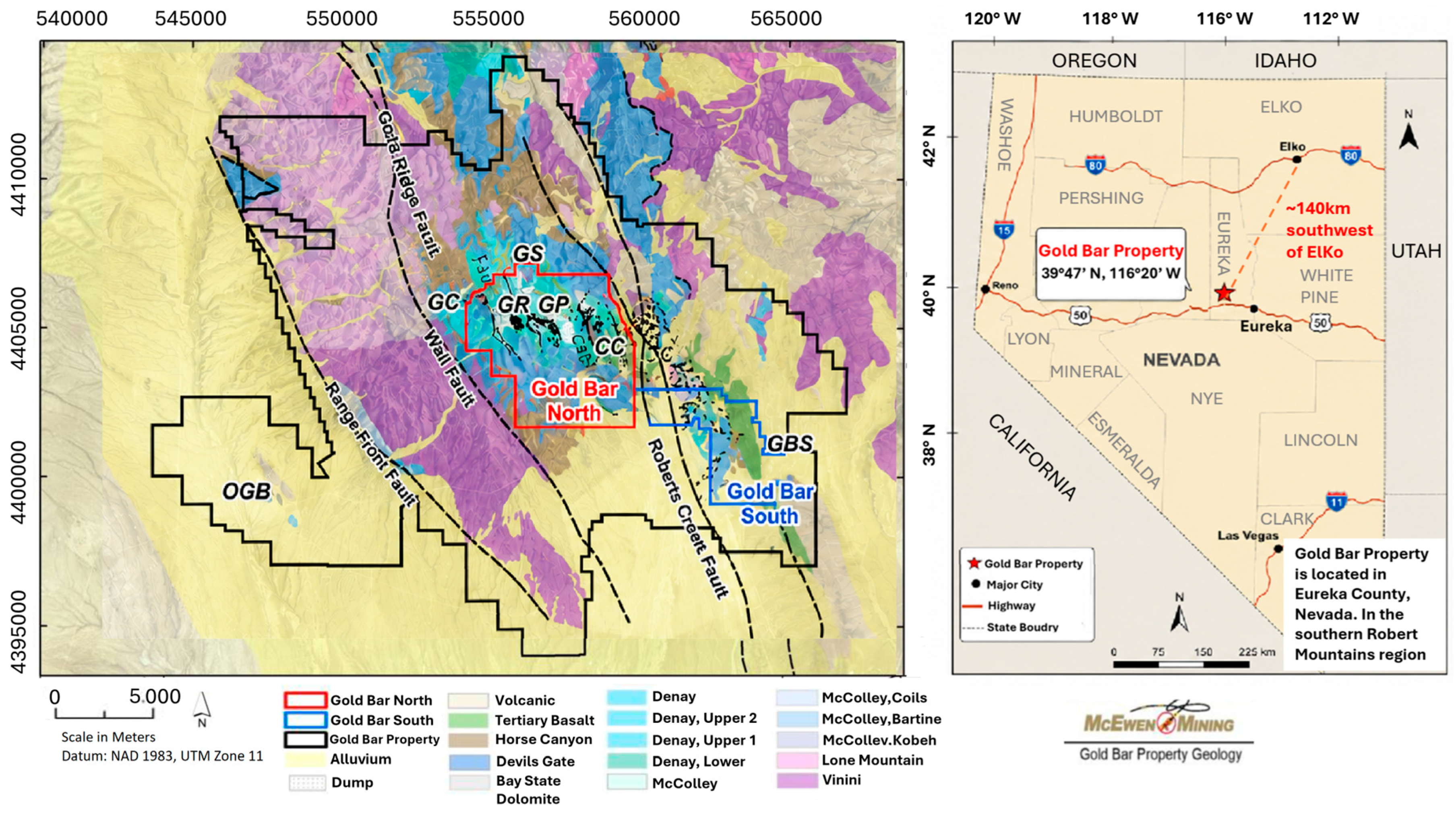
Figure 1. Gold Bar Property-Wide Geologic Map. Original Gold Bar Mine (OGB); Gold Canyon (GC); Gold Pick (GP); Goldstone (GS); Cabin Creek (CC); Gold Bar South (GBS), Modified from [39].
Minerals 16 00816 g001
Figure 2. Field Hyperspectral Imaging setup scanning pit walls labeled as (a) West Wall and (b) Pick 3.
Minerals 16 00816 g002
Figure 3. Local Spectra Library used to interpret clusters derived from the post-processing of hyperspectral data [42].
Minerals 16 00816 g003
Figure 4. Rock samples collected from the Gold Bar mine (GB north) for hyperspectral scanning in the lab.
Minerals 16 00816 g004
Figure 5. Overview of the workflow for hyperspectral pit wall mapping (Pick 3 dataset).
Minerals 16 00816 g005
Figure 6. Saturation analysis and image clipping for Pick 3. Red pixels: over-saturated regions. Blue rectangle: the selected analysis region to minimize the impact of oversaturation.
Minerals 16 00816 g006
Figure 7. Radiance-to-reflectance conversion and bad-band removal for the West Wall. Coloured polygons mark the Spectralon® calibration white reflectance panels (red: 20% reflectance; green: 50%) and delineate regions of interest used in empirical line correction.
Minerals 16 00816 g007
Figure 8. Selected PPI’s endmembers as reference spectra for SAM. The black circle shows the focused range (around 2000–2400 nm) with distinctive features for the Pick 3 pit wall.
Minerals 16 00816 g008
Figure 9. Methodology for deep learning-based classification using a combination of Autoencoder and K-means.
Minerals 16 00816 g009
Figure 10. Training and validation loss curves for the convolutional autoencoder applied to the Pick 3 pit wall. The shaded zone highlights the rapid convergence between Epochs 4 and 5.
Minerals 16 00816 g010
Figure 11. (a) VNIR RGB image of the Pick 3 pit wall, and unlabeled classification maps generated from SWIR data using three classification techniques: (b) SAM, (c) AE, and (d) BR. The corresponding mean spectra for each class identified by each method are also presented.
Minerals 16 00816 g011
Figure 12. Comparison between the mean spectra of the classified classes derived from each technique, SAM, BR, and AE, and the local reference spectra.
Minerals 16 00816 g012
Figure 13. Labeled classification maps of the Pick 3 wall were generated using three techniques, SAM, AE, and BR, based on similarity to local spectral references. The maps are shown alongside the schematic geological labels provided by the mine geologist.
Minerals 16 00816 g013
Figure 14. (a) VNIR RGB image of the West wall and unlabeled classification maps generated from SWIR data using three classification techniques: (b) SAM, (c) AE, and (d) BR.
Minerals 16 00816 g014
Figure 15. Labeled classification maps of the West pit wall generated using the SAM technique based on the mine geologist’s expertise.
Minerals 16 00816 g015
Table 1. Main specifications of the HySpex Mjolnir VS-620 imaging system.
V-1240S-620
Spectral range400–1000 nm970–2500 nm
Spatial pixels1240620
Spectral channels and sampling200 bands @ 3.0 nm300 bands @ 5.1 nm
F-numberF1.8F1.9
FOV20°20°
Pixel FOV across/along0.27/0.54 mrad0.54/0.54 mrad
Bit resolution (raw data)12 bit16 bit
Dynamic range440010,000
Max speed (at full resolution)200 fps170 fps
Table 2. Results of the XRD analysis of the 17 selected rock samples.
Mineral/Compound (WT%)GB1-1GB1-2GB1-3GB1-4GB1-5GB2-1GB2-2GB2-3GB2-4GB2-5GB3-1GB3-2GB3-3GB3-4GB3-5GB3-6GB3-7
Quartz10.837.92.645.816.432.923.337.638.192.69.40.610.214.026.051.392.7
Calcite63.90.883.023.359.414.831.67.15.10.160.584.331.459.233.12.60.2
Kaolinite0.30.9-0.81.31.30.50.40.60.20.70.10.7----
Pyrite0.00.4-0.30.30.41.80.30.3--0.11.0-0.9-0.2
Ankerite2.91.7-0.80.62.54.66.79.0-6.9-9.53.75.82.50.6
Dolomite9.730.9-3.23.012.313.124.626.5-13.3-20.56.910.114.10.0
Muscovite0.49.4-8.64.99.06.55.74.72.81.4-1.33.47.38.74.2
Siderite0.00.1-0.10.00.70.00.00.0---0.0----
Anatase0.10.2-0.20.20.30.30.10.2---0.2----
Orthoclase0.12.1-1.51.13.31.81.71.3---1.7-0.9--
Albite-1.7---1.90.50.60.7--------
Rutile--------------0.4--
Gypsum--------------1.0--
Dawsonite-----2.3-----------
Palygorskite-----2.71.92.41.6--------
Rhodochrosite------0.10.00.0----0.40.0--
Actinolite----------0.6----0.6-
Jarosite---------0.8-------
Barite----------------1.3
Amorphous Content11.713.914.415.412.915.613.912.811.83.67.214.923.612.414.420.30.8
TOTAL100100100100100100100100100100100100100100100100100
Table 3. Architecture of the convolutional autoencoder used in this study. Values in parentheses indicate kernel size. “Same” denotes the same padding, and ReLU denotes the rectified linear unit activation function.
Layer TypeOutput ShapeConfigurationPurpose
Input4 × 4 × 78N/AInput Layer
Conv2D4 × 4 × 16(1,1), ReLU, sameFeature Extraction
Conv2D4 × 4 × 16(3,3), ReLU, sameFeature Extraction
Conv2D2 × 2 × 32(3,3), ReLU, strides = 2, sameDownsampling
Conv2D2 × 2 × 32(3,3), ReLU, sameFeature Extraction
Conv2D1 × 1 × 64(3,3), ReLU, strides = 2, sameDownsampling
GlobalAvgPooling2D1 × 1 × 64N/ASpatial Compression
Dense128ReLULatent Representation
Dense128ReLULatent Expansion
Reshape1 × 1 × 128N/AReshape for Decoding
Conv2DTranspose2 × 2 × 64(3,3), ReLU, strides = 2, sameUpsampling
Conv2DTranspose4 × 4 × 32(3,3), ReLU, strides = 2, sameUpsampling
Conv2DTranspose4 × 4 × 16(3,3), ReLU, sameFeature Reconstruction
Conv2DTranspose4 × 4 × 78(1,1), Linear, sameFinal Reconstruction
Table 4. Band ratios * used for classification of Pick 3 (Wavelength in nm).
F1F2F3F4F5F6F7
2044/21622080/20242136/20242075/21002075/22182090/23412105/2218
F8F9F10F11F12F13F14
2136/22082141/22132182/21622182/23412233/22182136/21002233/2433
F15F16F17F18F19F20F21
2249/22182249/22742249/23362264/24332269/23462274/22032279/2208
F22F23F24F25F26F27F28
2279/23512300/22742300/24332305/23312331/22642331/24332377/2433
* Ratios are grouped by target absorption region: continuum/carbonaceous contrast 2000–2136 nm (F2, F3, F4, F13); Al–OH clay ~2160 nm (F1, F10); Al–OH illite/clay ~2200 nm (F5, F7, F8, F9, F12, F15, F20, F21); hydroxyl features ~2249–2300 nm (F14, F16, F23, F24); carbonate CO3 ~2330–2350 nm (F6, F11, F17, F18, F19, F22, F25, F26, F27, F28).
Table 5. The most similar spectrum from rock samples and the local spectra reference set for each class in SAM, AE and BR techniques on Pick 3.
Pick 3 SWIR_SAMPick 3 SWIR_AEPick 3 SWIR_BR
ClassesMost Similar SamplesMost Similar SamplesMost Similar Samples
Class 1GB3-4GB3-4GB3-4
Class 2GB3-5GB3-5GB3-5
Class 3GB3-5GB3-4GB3-5
Class 4GB1-1GB3-1GB1-1
Class 5GB3-4GB3-4GB3-4
ClassesMost Similar Local SpectraMost Similar Local SpectraMost Similar Local Spectra
Class 1Illite-CalciteIllite-CalciteIllite-Calcite
Class 2CarbonaceousCarbonaceousCarbonaceous
Class 3CarbonaceousIllite-CalciteCarbonaceous
Class 4Hematite–Quartz–CalciteIllite-CalciteHematite–Quartz–Calcite
Class 5Illite-CalciteIllite-CalciteIllite-Calcite
Table 6. Cosine similarity scores of the best-matching reference for each class, by technique and reference set (Pick 3).
ClassSAM
(Local)
AE
(Local)
BR
(Local)
SAM
(Sample)
AE
(Sample)
BR
(Sample)
Class 10.99830.99870.99870.99870.99940.9992
Class 20.99900.99890.99900.99950.99950.9995
Class 30.99880.99810.99840.99940.99920.9990
Class 40.99910.99870.99860.99660.99920.9974
Class 50.99870.99860.99870.99930.99920.9993
Table 7. Summary similarity and separation-margin statistics per technique (Pick 3).
MetricSAMAEBR
Mean similarity score (Local)0.99880.99860.9987
Mean similarity score (Sample)0.99870.99890.9987
Mean separation margin (Local)0.000790.000360.00079
Mean separation margin (Sample)0.000160.000160.00014
Distinct reference labels resolved (of 5, Local)323
Table 8. Cross-technique agreement on best-match class labels, by reference set (Pick 3).
ComparisonAgreement (Local)Agreement (Sample)
SAM vs. BR5/5 (100%)5/5 (100%)
SAM vs. AE3/5 (60%)3/5 (60%)
BR vs. AE3/5 (60%)3/5 (60%)
Table 9. Polygon-wise correspondence between geologist interpretation and dominant hyperspectral classes for the Pick 3 wall.
PolygonGeologist InterpretationAE Dominant/ConsistencySAM Dominant/ConsistencyBR Dominant/Consistency
1Carbon/TanCarbonaceous (54.3%) consistentCarbonaceous (65.3%) consistentCarbonaceous (62.4%) consistent
2Carbon/TanIllite–Calcite (58.6%) consistentIllite–Calcite (42.9%) consistentCarbonaceous (46.3%) consistent
3Carbon/BrownCarbonaceous (69.4%) consistentCarbonaceous (83.8%) consistentCarbonaceous (75.4%) consistent
4Tan/RedIllite–Calcite (90.7%) consistentIllite–Calcite (58.8%) consistentIllite–Calcite (51.8%) consistent
5Brown/CalciteIllite–Calcite (69.1%) consistentIllite–Calcite (45.7%) consistentIllite–Calcite (51.0%) consistent
6Calcite/CarbonIllite–Calcite (84.3%) consistentCarbonaceous (56.8%) consistentIllite–Calcite (48.0%) consistent
7Red/BrownIllite–Calcite (77.3%) partially consistentIllite–Calcite (74.9%) partially consistentIllite–Calcite (69.2%) partially consistent
8Carbon/CalciteIllite–Calcite (78.5%) consistentIllite–Calcite (26.7%) consistentHematite–Quartz–Calcite (28.9%)
weak/mixed consistency (BR split between calcite/carbonate and hematite-bearing class; mixed correspondence)
9Calcite/CarbonCarbonaceous (72.3%) consistentCarbonaceous (81.9%) consistentCarbonaceous (75.5%) consistent
10Carbon/TanCarbonaceous (71.0%) consistentCarbonaceous (76.1%) consistentCarbonaceous (72.9%) consistent
Disclaimer/Publisher’s Note: The statements, opinions and data contained in all publications are solely those of the individual author(s) and contributor(s) and not of MDPI and/or the editor(s). MDPI and/or the editor(s) disclaim responsibility for any injury to people or property resulting from any ideas, methods, instructions or products referred to in the content.