Resource Assessment with Uncertainty Quantification of Intrusive Orebodies Using Level Sets with Stochastic Motion: Application to a Shear-Hosted Copper Deposit

Abstract

Mining project evaluation depends on geological resource models, yet these models remain inherently uncertain because they are constructed from sparse drillhole data, indirect geophysical observations, and incomplete geological knowledge. Conventional workflows typically treat this uncertainty only partially by defining deterministic orebody wireframes and then interpolating or simulating grades within these fixed boundaries. This separation neglects the propagation of geometric uncertainty into grade continuity, resource tonnage, and economic forecasts. The challenge is particularly significant where drillholes do not fully intersect the orebody, leaving its extent at depth unconstrained and forcing boundary placement to rely on extrapolation rather than data-supported inference. To overcome this limitation, we present a sequential uncertainty quantification framework that integrates level-set implicit geological modeling within a Markov Chain Monte Carlo (MCMC) sampler with Sequential Gaussian Simulation (SGSIM) grades. Orebody geometry is represented using a signed distance function perturbed by Gaussian random fields and constrained by drillhole, outcrop, and geological interpretation data. The resulting ensemble captures plausible geometric variability, particularly in poorly constrained regions. Conditional grade simulations are then generated for each accepted geometry, producing paired realizations of geometry and grade uncertainty. Applied to the Tarmante copper deposit in Morocco, the framework demonstrates that deterministic models overestimate tonnage, whereas the joint ensemble provides realistic grade–tonnage uncertainty, enabling more reliable resource evaluation and risk-informed decision-making.

1. Introduction

Geological resource modeling provides the foundation for evaluating mineral deposits and guiding decisions in exploration and mining. Nevertheless, the true geometry, size, and grade distribution of a deposit remain unknown until the resource has been fully extracted [1,2]. In practice, models are constructed from incomplete observations, limited drillhole data and indirect geophysical surveys, which together provide only a fragmented view of the subsurface. Historically, these resource models have been constructed deterministically by geologists who leverage their knowledge and the available data to create a single, best-guess representation of the subsurface. However, the natural complexity and heterogeneity of geological systems mean that such models often fall short of capturing the true extent of subsurface uncertainties and variability [3,4,5,6,7,8]. If geological uncertainty is not explicitly accounted for, it propagates into resource estimates, mine planning, economic evaluations, and decision-making processes, potentially leading to significant financial losses [2,9,10,11].

Within this context, resource modeling is generally framed around two main aspects: first, identifying the geological factors that control mineralization [12]; and second, applying quantitative interpolation techniques to estimate mineral content from assay data. Geostatistical methods, particularly kriging and its variants, have long been used as standard tools for spatial interpolation [5,13]. These methods provide point estimates in areas without direct observations but remain limited in their capacity to represent spatial uncertainty in complex geological settings. Stochastic simulation techniques have been developed to address these limitations. Sequential Gaussian simulation (SGS) is commonly applied for this purpose [14,15], with early studies demonstrating its application in evaluating grade–tonnage risk and the implications for feasibility studies and mine design [16]. Subsequent work extended these methods to assess the influence of grade uncertainty on production scheduling [17]. Further contributions extended these approaches to resource classification, supporting the differentiation of measured, indicated, and inferred categories [18]. Conditional simulations have also been applied to grade estimation under soft geological boundaries, highlighting their role in representing uncertainty where geological constraints are less defined [19]. Holding the geology fixed while simulating grades alone fails to address uncertainty related to the shape or extent of the orebody, potentially leading to underestimated risk [20]. To capture geometric variability, researchers extended stochastic approaches to orebody geometry, wireframes, and domain boundaries. For example, sequential indicator simulation (SIS) was applied to evaluate uncertainty in ore volumes and mineralized zones [21,22]. Plurigaussian simulation was introduced to better reproduce geological controls on lithological and grade domains and has since been applied to a wide range of deposits, including copper, uranium, kimberlite, nickel laterite, gold, and lead–zinc systems [23,24,25,26,27,28,29,30]. Truncated Gaussian simulation was tested in porphyry copper and sedimentary systems [31,32]. To overcome the restrictions of two-point statistics, higher-order methods emerged, notably training-image–based multiple-point statistics (MPS) [33,34,35,36]. These methods are applied to uncertainty in lithological models and volumetric variability in deposits such as Yandi iron ore (channel iron deposit), and the Olympic Dam deposit (iron oxide copper–gold, IOCG) [33,37]. Joint simulation of grade and geometry further extended these ideas, with applications to grade–tonnage risk and financial evaluation [38], soft-boundary grade estimation [19,39], and boundary uncertainty in copper and iron deposits [40,41,42].

Recently, probabilistic frameworks using level-set methods have been developed for stochastic domain modeling. Ref. [43] proposed a level-set framework in which lithological boundaries are represented as random implicit functions decomposed into a stochastic trend and a residual component; uncertainty is propagated through probability perturbation and conditional simulation, producing multiple equiprobable realizations of 3D domain boundaries in a porphyry copper deposit [44] introduced a data and knowledge-driven trend surface analysis in which geological interfaces are represented as level-set functions perturbed within a Metropolis–Hastings framework, integrating boreholes, geophysics, and geological sketches to quantify uncertainty in subglacial topography, magmatic intrusions, and palaeovalleys [44]. Knowledge-driven stochastic geometry modeling by embedding 2D geological sketches directly into a level-set Monte Carlo framework, where Procrustes analysis was used to enforce geometric similarity, applied to the Crystal Lake Gabbro intrusion [45].

Despite these advances, most resource modeling workflows still handle grade and geometry uncertainty separately, with domains usually defined deterministically through wireframes or grade shells before grade simulation. In such workflows, geometry does not contribute to the modeling uncertainty [45].

In this paper, we develop a novel approach to the sequential quantification of uncertainty in the geometry and grade distribution of a copper orebody intrusion in the Anti-Atlas region of Morocco. The geometry is constrained by drillholes and outcrop contacts. The geological conceptual model will be integrated through a geological sketch of the 2D intrusion intersection. The framework explores extrapolating orebody geometry beyond the data support, where observations alone are insufficient to constrain the full extent of the intrusion. For the accepted intrusion geometries, a conditional 3D grade realization is simulated to link geometry and grade uncertainty. This sequential modeling enables the quantification of uncertainty in grade-tonnage curves, providing a probabilistic basis for exploration targeting and resource evaluation.

2. Materials and Methods

Our methodology uses a level set approach and its stochastic perturbation [45,46,47] to quantify and visualize the uncertainty of subsurface orebody geometry. We incorporate information from drillholes, outcrop contacts, and geological sketches by defining loss functions that measure the mismatch between model outputs and data. Additionally, we use geostatistical simulation to model copper grade variability within the generated geometry. This section outlines the construction of the level set framework, the incorporation of geological constraints, and the process by which uncertainty is propagated through model realizations.

2.1. Uncertainty Quantification on Intrusive Bodies

2.1.1. Geometry Representation Using Level Sets

We model the geometry of the copper intrusion using a level-set methodology that combines data and knowledge-driven modeling and is developed in detail in [45,48].

The level set representation of the intrusion geometry is achieved by formulating the orebody interface as a signed distance function defined on a regular three-dimensional grid. This approach encodes the spatial configuration of the mineralizing fluid intrusion boundary not through discrete surface elements, but via a scalar field $\varnothing \left(x\right)$ where each grid point x (x, y, z) stores the minimum distance to the nearest point on the interface. The sign of $\varnothing \left(x\right)$ provides a binary classification of space: interior or exterior to the orebody.

Formally, the function is defined as:

$$\mathrm{\varnothing }(x)=\left\{\begin{array}{c}<0,ifxliesinsidetheintrusion\\ =0,ifxliesontheinterface\\ >0,ifxliesoutsidetheinterface\end{array}\right.$$

(1)

This signed distance field allows handling complex geometries. Constraining the level sets to various data sources is done by perturbing some initial guess until an objective associated with the type of data is met. The perturbation of the interface is governed by the level set equation and the definition of a velocity field, $v^{\ast }\left(x\right)$:

$${\mathrm{\varnothing }}^{n+1}={\mathrm{\varnothing }}^n-\left(v^{\mathrm{\ast }}\left|\nabla {\mathrm{\varnothing }}^n\right|\right)∆t,$$

(2)

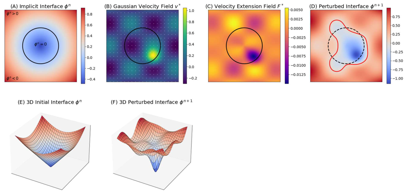
In our implementation, the velocity field $v^{\ast }\left(x\right)$ is drawn from a stationary Gaussian process. The full perturbation process is illustrated in Figure 1, which summarizes the evolution of the signed distance function across a single iteration. Figure 1A shows the initial configuration $\varnothing \left(x\right)$, where the black contour delineates the interface $(\varnothing =0)$ separating the orebody from the surrounding host rock. Figure 1B visualizes a realization of the sampled Gaussian velocity field $v^{\ast }$, in which vector magnitude and direction encode spatially variable perturbation patterns. This velocity is then extended along the normal direction to the interface, producing a smooth velocity extension field $F^{\ast }$ (Figure 1C). The perturbed surface is represented by the red line, and the dashed black line shows the original geometry for comparison (Figure 1D). Figure 1E,F provides a volumetric perspective of the signed distance field before and after perturbation, revealing the localized deformation of the geometry.

2.1.2. Incorporating Data and Knowledge Through a Loss Function Design

To simulate subsurface intrusion, we constrain the level set evolution to a set of geoscientific data. These include lithological indicators from drillholes (n = 138), outcrops (n = 481) observed at the surface, and a 2D geological sketch interpreted to represent a cross-section of the intrusion. These data contribute a distinct type of spatial information and are integrated into our probabilistic modeling framework via a set of loss functions.

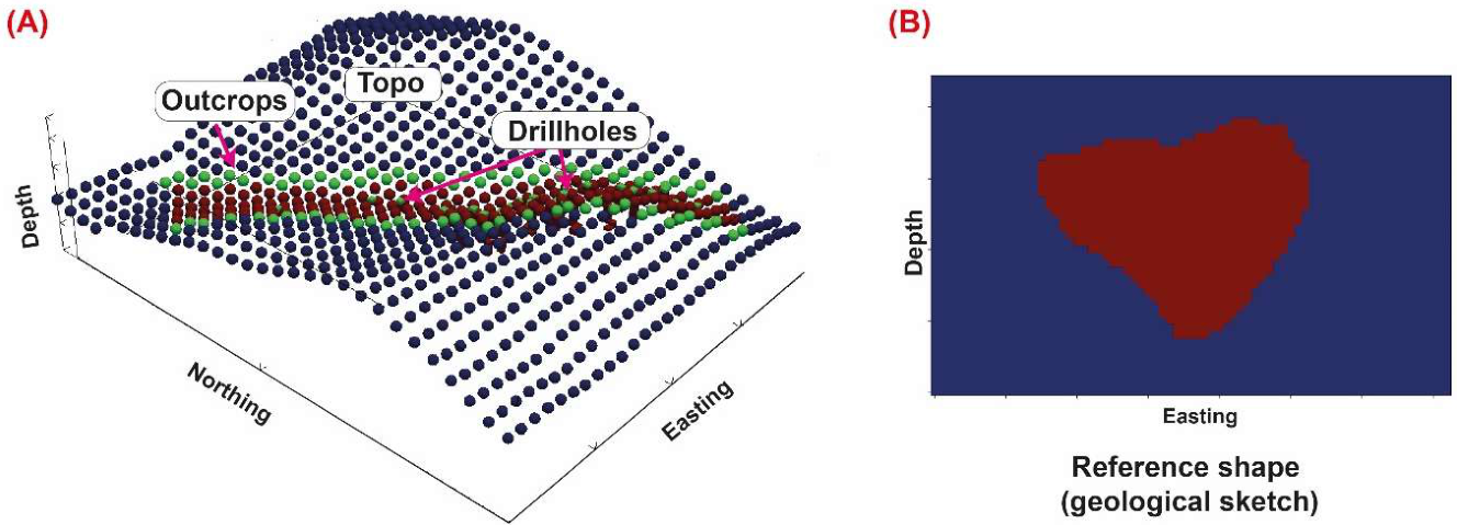
The data are first converted into a common format and aligned with the supporting 3D modeling grid. Drillholes, outcrops, and topographic points are assigned categorical values: 1 for intrusive, 0 for non-intrusive, and 0.5 for contact zones (Figure 2A). Geological sketches are projected onto 2D model slices and aligned using Procrustes analysis (see [45] for details). This alignment allows the sketch to guide the shape of the modeled interface, bringing conceptual geological structure into the quantitative modeling process (Figure 2B) [45]. In this case, none of the drillholes intersect the bottom of the mineralized intrusion, leaving the lower extent of the orebody unconstrained. As a result, the depth and extent of the intrusion remain uncertain and should not just be modeled using a deterministic interpolation. These different data types are combined into a single input used to compare model outputs against observations.

Once all geological inputs are encoded and aligned with the 3D mesh, we evaluate each model realization by comparing its predicted geometry to the observed data. This comparison is done through a set of loss functions, each corresponding to a specific data type: drillhole lithology, contact locations, outcrop data and geological sketch. Each function measures how well the model satisfies that constraint. The total misfit is expressed as a weighted combination of these individual losses:

$$L_{total}=W_b{L}_b+W_c{L}_c+W_p{L}_p,$$

(3)

where $W_b$, $W_c$, and $W_p$ are weights assigned to drillhole data, outcrops, and sketches, respectively. $L_b$, $L_c$ and $L_p$ are the loss functions for the drillhole, contact, and sketch constraints, respectively.

Drillhole and outcrop lithologies are encoded as 1 (intrusion) or 0 (non-intrusion). If the model predicts a signed distance function $\varphi \left(x\right)$, correct classification means $\varphi \left(x\right)<0$ for intrusive and $\varphi \left(x\right)>0$ for non-intrusive points. To measure classification mismatch, the binary loss is defined using a smooth logistic function:

$$L_b={\sum }_{x_i\in intrusion}log\left(1+exp\left(-\varphi \left(x_j\right)\right)\right)+{\sum }_{x_i\in non-intrusion}log\left(1+exp\left(\varphi \left(x_i\right)\right)\right),$$

(4)

where $x_i$ and $x_j$ are the spatial locations of intrusive and non-intrusive observations, respectively.

The logistic function provides a smooth measure of misclassification, allowing the model to adjust gradually as points move away from their expected position relative to the interface.

For the boundary between intrusive and non-intrusive zones, we use the mean squared residual and squared mean error to quantify model variance and bias at outcrops:

$$L_c={\displaystyle \frac{1}{n_c}}{\displaystyle {\sum }_{i=1}^{n_c}}(0-\varphi \left(x_i\right){)}^2+({\displaystyle \frac{1}{n_c}}{\displaystyle {\sum }_{i=1}^{n_c}}(0-\varphi \left(x_i\right)){)}^2,$$

(5)

where $\varphi \left(x_i\right)$ is the signed distance function, which is evaluated at the contact point x_i, n_c is the total number of outcrop contact points, $x_i$ ∈ R³ denotes the spatial coordinates of the ith contact point.

Geological sketches are incorporated as shape constraints following the approach of [45]. Model-derived cross-sections are aligned with reference sketches using Ordinary Procrustes Analysis [49,50], which applies a combination of translation, rotation, and scaling. The misfit is computed as the squared Frobenius norm between the aligned shapes:

$$L_p\left(X_1,X_2\right)={‖X_2-\beta X_{1}R-C‖}^2,$$

(6)

where X₁ and X₂ are reference and comparison shape matrices, β is a scaling factor, R is a rotation matrix, and C is a translation vector.

2.1.3. Sampling of Intrusive Body Realizations

Stochastic perturbations are made to the surface until they honor the above loss functions. Such perturbations are gradual and such that they are reversible to obtain convergence. To do so, we apply a Markov Chain Monte Carlo (MCMC) framework to generate an ensemble of intrusion geometries consistent with geological observations [51,52], which iteratively proposes perturbations to the current model and accepts or rejects them based on a data-informed acceptance criterion. As explained above, each proposal is generated by applying a velocity field, sampled from a stationary Gaussian process, to perturb the signed distance function $\varnothing$ via the level set evolution equation. This process produces a new candidate geometry that reflects both the underlying geological variability and the imposed spatial constraints. At each iteration, the total loss $L_{total}$ is computed for the proposed model and compared to that of the current model. The acceptance criterion α is defined as:

$$\alpha =min\left(1,\exp (-\left[L_{total}^{\left(j\right)}-L_{total}^{\left(i\right)}\right]/\mathrm{T})\right),$$

(7)

where $L_{total}^{\left(i\right)}$ and $L_{total}^{\left(j\right)}$ are the total losses for the current and proposed models, respectively. T is a fixed temperature parameter that relaxes the acceptance criterion by increasing the probability of accepting moderately higher-loss proposals. If the proposed model yields a lower loss, it is accepted with higher probability. Accepted realizations are retained, forming a posterior distribution of geometries that approximately satisfy the geological constraints.

2.1.4. Grade Simulation and Uncertainty Quantification

In addition to uncertainty in the intrusion geometry, the 3D distribution of copper grade within the model needs to be modeled as well. Here we adopt a traditional geostatistical approach using sequential Gaussian simulation, but each realization is performed within a single simulated intrusive body identified by the condition $\varnothing \left(x\right)<0$. Copper grade is modeled as a scalar field Z(x), where x ∈ R³ denotes a location within the regular 3D simulation grid.

The dataset consists of 3859 assayed copper samples, each 1 m in length, analyzed by atomic absorption spectroscopy (AAS) at the Ohod Mining Company laboratory. Copper grade is modeled as a multivariate Gaussian random field, a common geostatistical practice in mineral resource estimation. To characterize the spatial continuity of copper concentration, we first apply a normal score transformation to the drillhole assay data, mapping the original grade values to a standard normal distribution. This transformation enables the use of simulation methods that assume Gaussian behavior. To generate grade realizations, we use Sequential Gaussian Simulation (SGSIM).

2.2. Synthetic Case Study Assessing Geometry Extrapolation Under Data Sparsity

One of the central challenges in modeling intrusive orebodies is constraining geometry below the deepest drillhole intersection. When all drillholes return positive lithological indicators throughout their full lengths, the basal boundary is not constrained by the data. Deterministic models address this by placing the contact at or near the deepest intersection, guided by geological judgment [5], though the resulting boundary reflects interpreter assumptions as much as the data themselves. While previous work has shown that geometric uncertainty can be quantified and propagated where drillhole observations exist [53], and that integrating geological knowledge through sketch-based priors helps constrain interfaces in data-sparse regions [43,44,45], the specific problem of extrapolating geometry into regions entirely devoid of observations, such as the unconstrained basal boundary of an intrusion, remains largely unexplored. The level-set MCMC framework addresses this by coupling a geometric shape prior with the conditioning data, allowing the posterior ensemble to explore geometries consistent with both, including those extending well below the data support.

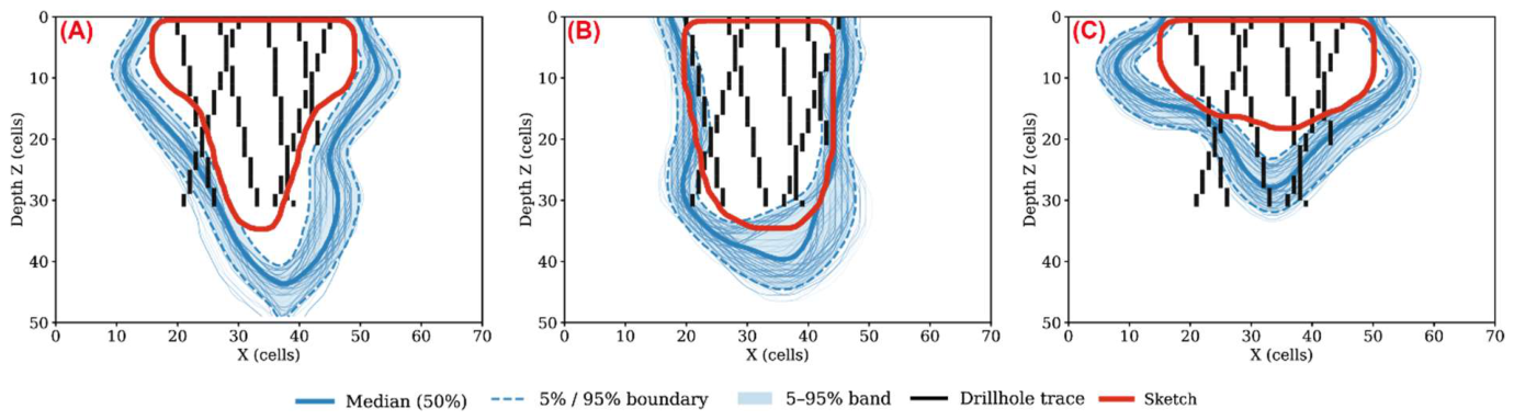
To demonstrate this, a synthetic case study was designed on a regular 2D grid of 70 × 50 cells representing a vertical cross-section of an intrusive orebody, mimicking a realistic exploration scenario in which the depth extent of the intrusion is unknown. Surface outcrop contacts constrain the lateral extent at the surface, and three data scenarios are tested corresponding to 4, 5, and 6 drillholes; in each scenario, all drillholes penetrate the upper portion of the intrusion without intersecting the lower contact. The approach proceeds sequentially: sketch falsification, variogram range falsification, and then full posterior inference, so that every modeling assumption is tested against the data before being used as input. For the sketch falsification, three candidate sketches representing distinct geological interpretations of the intrusion cross-section were each run through the level-set MCMC and evaluated against the drillhole data. A sketch is rejected if the drillhole observations fall outside the posterior boundary ensemble, that is, if the modeled intrusion fails to contain the observed drillhole intersections. As shown in Figure 3, Sketches A and C are falsified: in both cases the posterior ensemble does not consistently enclose the drillhole data, indicating that these geometries are incompatible with the observations. Only Sketch B with a U-shaped geometry produces a posterior in which all drillhole intersections fall within the modeled intrusion, and it is therefore retained as the geometric prior for all subsequent analysis.

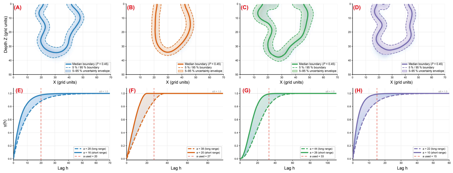
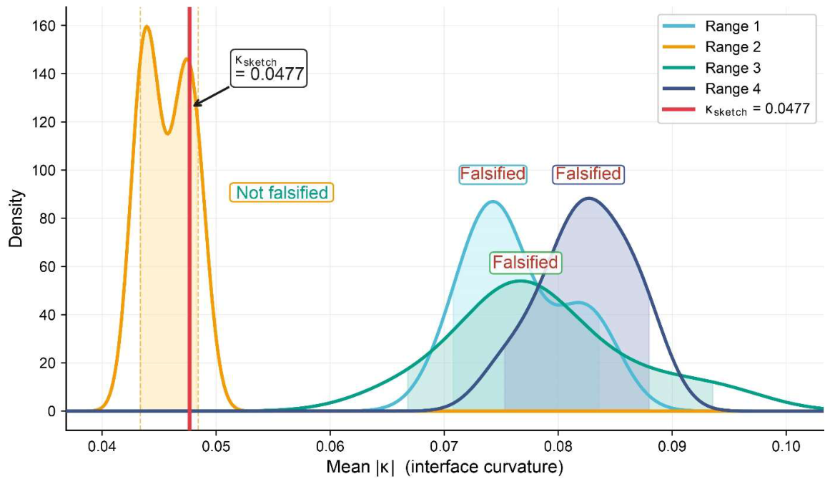
With the sketch prior established, the next modelling decision is the variogram range parameter governing the spatial smoothness of the Gaussian perturbation field. Four candidate range configurations were tested (Range 1: a = 16–28; Range 2: a = 20–38; Range 3: a = 26–44; Range 4: a = 10–22), and for each, the mean absolute curvature |κ| = |dθ/ds| was computed across all posterior realisations and compared to the reference value κ_sketch = 0.0477 derived from the accepted sketch (Figure 4).

A range configuration is falsified if the reference falls outside the distribution of its posterior curvature values. As shown in Figure 4 and Figure 5, only Range 2 (a ∈ (20, 38) cannot be falsified; its posterior curvature distribution is the only one that contains κ_sketch = 0.0477, confirming that the geometries it produces are statistically consistent with the accepted sketch. Ranges 1, 3, and 4 are all falsified, their curvature distributions concentrated well above the reference value between 0.07 and 0.09, meaning the interfaces they generate are systematically too rough relative to the sketch geometry (Figure 4). Range 2 is therefore carried forward into all subsequent inference.

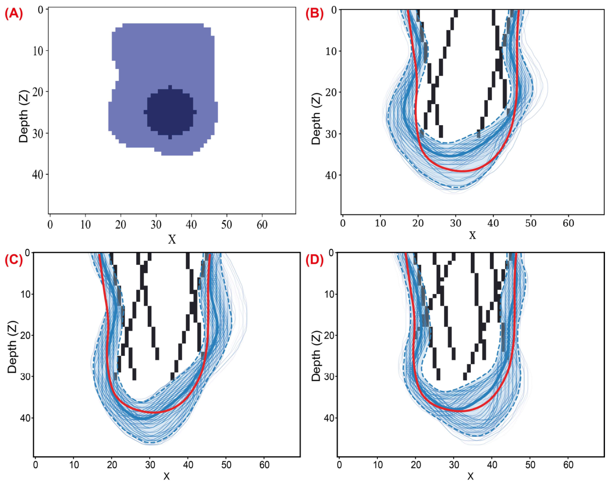
With both the sketch prior and variogram range established through falsification, the full inference was run for all three data scenarios 4, 5, and 6 drillholes over 6000 MCMC iterations each, using the accepted sketch, the selected variogram range, and the available outcrop contacts. The initial model and accepted sketch are shown in Figure 6 alongside the posterior ensembles for each data scenario. In all three scenarios, the posterior realizations consistently enclose the drillhole observations, confirming that the accepted sketch and variogram range produce geometries compatible with the data (Figure 6). In the shallow and lateral regions, where drillhole and outcrop contacts provide direct geometric information, the ensemble is well concentrated, and the realizations converge toward a consistent boundary position. As data density increases from 4 to 6 drillholes, the ensemble narrows further in these constrained regions, reflecting the additional geometric information each new observation contributes. The reference geometry in the red contour is bracketed by the realizations in all scenarios, confirming that the posterior is well calibrated.

At depth, below the deepest drillhole intersection, the picture changes. The ensemble fans out substantially and assigns probability mass to a wide range of depth extents, with the maximum plausible depth remaining comparable across all three scenarios. The region of maximum spread at depth is precisely where a follow-up observation would have the greatest impact, whether a drillhole designed to exit the intrusion or a geophysical survey sensitive to its lower extent.

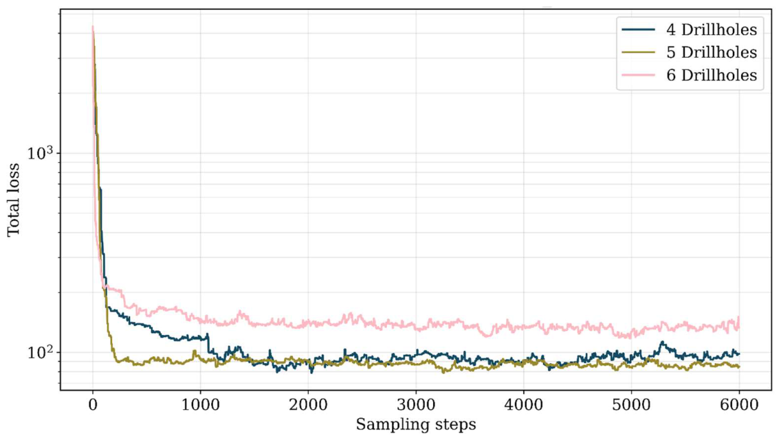
Figure 7 shows the total loss as a function of the number of sampling steps for all three scenarios. All three chains drop sharply during the first 300–500 iterations, the burn-in phase, as the model moves from the prior-informed starting configuration toward data-consistent geometries. After this initial adjustment, the loss stabilizes and fluctuates around a stationary value, confirming convergence. The 6-drillhole scenario maintains a higher stationary loss than the 4- and 5-drillhole cases, as expected: more observations impose more constraints that must be satisfied simultaneously, raising the minimum achievable misfit. The 4 and 5-drillhole chains reach comparable stationary levels, consistent with the similar posterior spread observed in those two scenarios.

Together, the three scenarios confirm that the level-set MCMC framework produces calibrated, geometrically consistent posteriors that correctly reflect what the data constrain and what they do not. The sequential falsification of sketch and variogram range ensures that all modelling assumptions are tested against observations before being used as inputs, replacing subjective judgment with a reproducible procedure. This validated framework is now applied to the Tarmante copper deposit in the Eastern Anti-Atlas of Morocco.

3. Results and Discussion

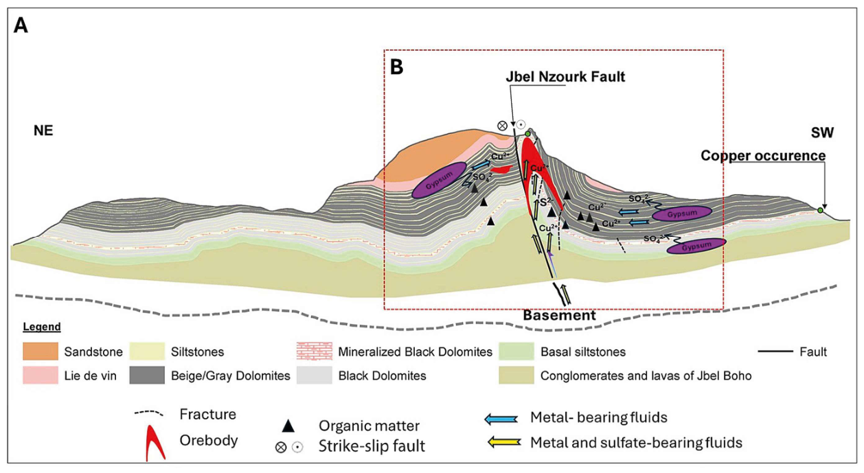
The Tarmante copper deposit, located in the Eastern Anti-Atlas of Morocco, is classified as a sediment-hosted copper system. Mineralization is structurally controlled, associated with a fault network and concentrated within a shear zone, where deformation created pathways for fluid flow and ore deposition. The main host lithologies are dolomitic limestone and siltstone, which occur as disrupted and displaced blocks inside the shear zone rather than as continuous stratigraphic units. As illustrated in Figure 8A (from [53]), copper can occur in a stratiform style broadly following dolomite and siltstone layers, whereas Figure 8B highlights the structural reworking of mineralization, where the Jbel N’Zourk fault and associated fractures acted as fluid drains and localized copper across multiple lithologies. The Tarmante occurrence shows a comparable setting, where copper is similarly concentrated in structurally prepared zones rather than strictly following stratigraphy. As in Jbel N’Zourk, the Tarmante mineralization shows the structurally reworked zones (Figure 8B), with the latter dominating the shear-hosted mineralization modeled in this study. Thus, mineralization in both cases is localized where structural features intersect permeable or chemically favorable units within the deformed zone, while the surrounding stratiform units outside this structural corridor show no mineralization. This clear spatial separation supports treating the contact between the shear-hosted intrusive mineralization and the host rocks as a hard boundary in the modeling workflow.

We employed a level-set representation of the geometry, modeling the target boundary as the zero-level isosurface of a scalar field, defined as a signed distance function. The initial level-set field was constructed as a smooth signed distance to a geometrically regular ellipsoid, which serves as a simple volumetric prior (Figure 9A). This ellipsoid acts as a starting point, ensuring symmetry and topological continuity while remaining flexible to data-driven deformation.

Subsequent perturbations to this initial surface were introduced through a stationary Gaussian field (

Table 1. Parameters used for Gaussian field perturbations and MCMC sampling in level set modeling.

Index	Variable	Description	Range/Value	Type
1	mean	Mean of the Gaussian perturbation field	0	Constant
2	variance	Variance of the Gaussian perturbation field	1	Constant
3	range_x	Variogram range in x-direction (Easting)	10–50	Uniform
4	range_y	Variogram range in y-direction (Northing)	10–50	Uniform
5	range_z	Variogram range in z-direction (Depth)	5–50	Uniform
6	anisotropy_xy	Anisotropy angle in the xy-plane	0–180°	Uniform
7	anisotropy_xz	Anisotropy angle in the xz-plane	0–180°	Uniform
8	max_step	Maximum perturbation step size	2	Constant
9	Wb	Weight on drillhole loss term	1	Constant
10	Wc	Weight on outcrop/surface loss term	1	Constant
11	Wp	Weight on geological sketch	50	Constant
12	temperature	Temperature parameter for MCMC sampling	300	Constant
13	iterations	Number of MCMC iterations	10,000	Constant

). These perturbations represent deviations from the ellipsoidal baseline and are designed to explore the space of alternative geometries that are consistent with the data. The Gaussian field follows a multi-Gaussian prior with a prescribed covariance structure, as the true spatial continuity of the geological interface is unknown (Table 1). As noted by [43], the implicit function’s covariance cannot be inferred directly from sparse data, so it must be treated as a hyperparameter reflecting structural assumptions. We selected the horizontal range to be at least as large as the largest gap between hard data points, based on the principle that shorter ranges can introduce high-frequency variations in areas with limited data [43,44]. Studies have shown that small correlation lengths in level-set perturbations can lead to local oscillations and slow MCMC convergence in data-sparse regions [43]. By using larger ranges, each proposed update results in broader surface adjustments that align with the geological scale of variation, avoiding unrealistic local changes [44].

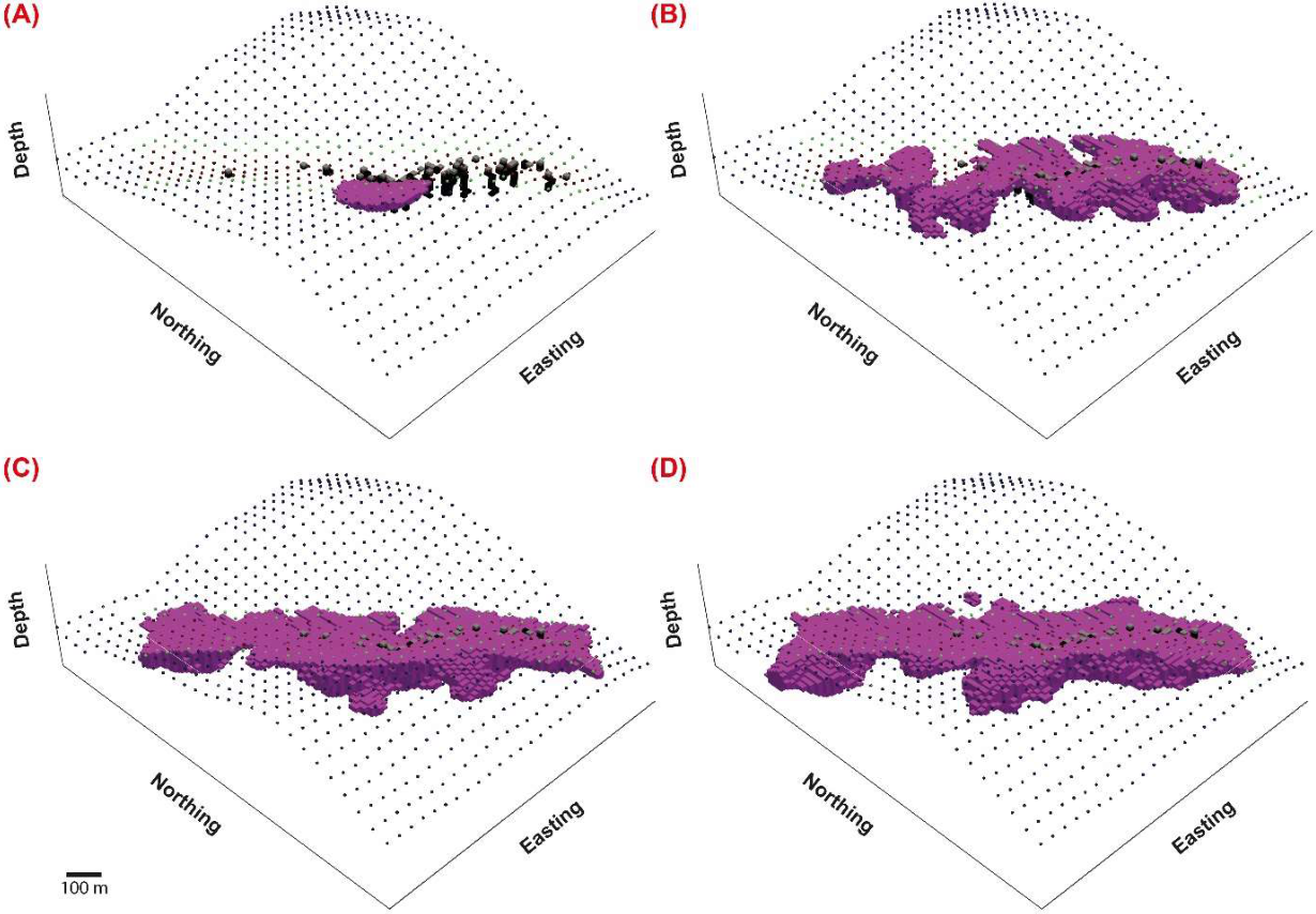
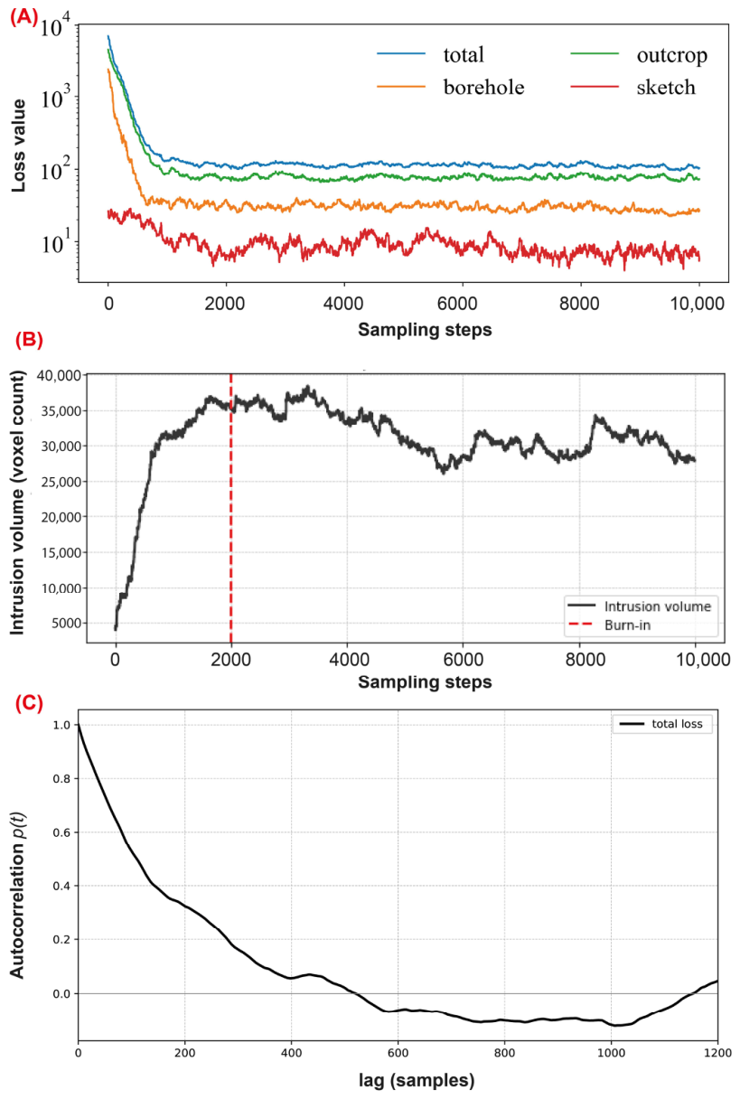
The perturbation magnitude is calibrated using a step-size factor Δt, which scales the Gaussian perturbation added to the level-set at each MCMC step. If Δt is too large, proposals are frequently rejected, and if it is too small, the chain mixes slowly. We set Δt = 20 m, and the MCMC algorithm was run for 10,000 iterations. Convergence was assessed by monitoring the stabilization of the loss function components across iterations, while the sampling efficiency is reflected by an acceptance rate of approximately 0.46. The grid was discretized into 73 × 85 × 45 cells with voxel dimensions of 10 m (x, y) and 5 m (z). The initial segment of the chain is defined as the burn-in phase (Figure 10A), during which the model transitioned from the prior-informed initial guess (Figure 9A) toward configurations more consistent with the observed data. This transition is visible in the loss function trajectory that decreases during the first few hundred iterations, reflecting substantial improvements in the geometrical fitting (Figure 10A). By approximately iteration 1000, the loss curve begins to flatten, where models are starting to take shape as shown in Figure 9C, and by iteration 2000, it stabilizes into a plateau with only minor fluctuations (Figure 9D). As also shown in Figure 10B, the intrusion volume increases rapidly during the early iterations as the model departs from the prior-informed initial geometry, and subsequently fluctuates within a stable range after approximately 2000 iterations, consistent with the burn-in identified from the loss trajectories. This behavior indicates that the sampler had reached the high-probability region of the posterior distribution and subsequent samples primarily explored local variations (Figure 10A).

The trajectory, shown in Figure 10A, thus provides a clear diagnostic of convergence, with the burn-in phase effectively concluded within the first 1000–2000 iterations. After the burn-in phase, Figure 11 shows modes from the last 1000 posterior geometry realizations as 3D surfaces, illustrating both variability and structural coherence. The intrusion volume after burn-in fluctuates within a stable range, indicating that the Markov chain is exploring alternative geometrical configurations (Figure 10B). We assessed convergence using the autocorrelation of the total loss. We computed ρ(t) after burn-in (Figure 10C). It drops from 1 to below 0 within about 500 steps. We kept realizations spaced wider than this for the reported ensemble. All realizations define a single, continuous subsurface interface with smooth curvilinear geometry, free of geologically implausible artifacts.

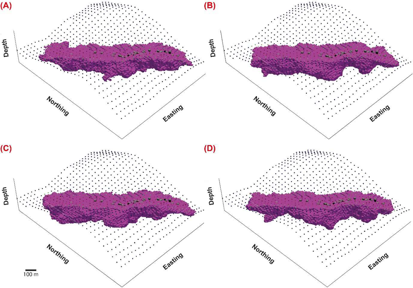
Unlike pixel-based methods (e.g., SIS), which can yield noisy or discontinuous results [6], the level-set MCMC approach generates geologically realistic alternatives that differ primarily in position, not structure (Figure 11A–D), consistent with the behavior also observed by [43]. This consistency reinforces confidence in the ensemble and ensures the sampled variability is a meaningful representation of geological uncertainty, not an artifact of the modeling technique. All posterior realizations honor the conditioning data by design. The likelihood function penalizes misfit at known borehole and outcrop locations, ensuring that accepted models closely match these constraints. This is achieved using a smooth logistic loss, which strongly discourages sign errors or large offsets while still allowing theoretical flexibility for data integration. This behavior parallels that of [43], who enforced zero-mean residuals at contacts, and [44], who used similar penalty functions to preserve geological realism.

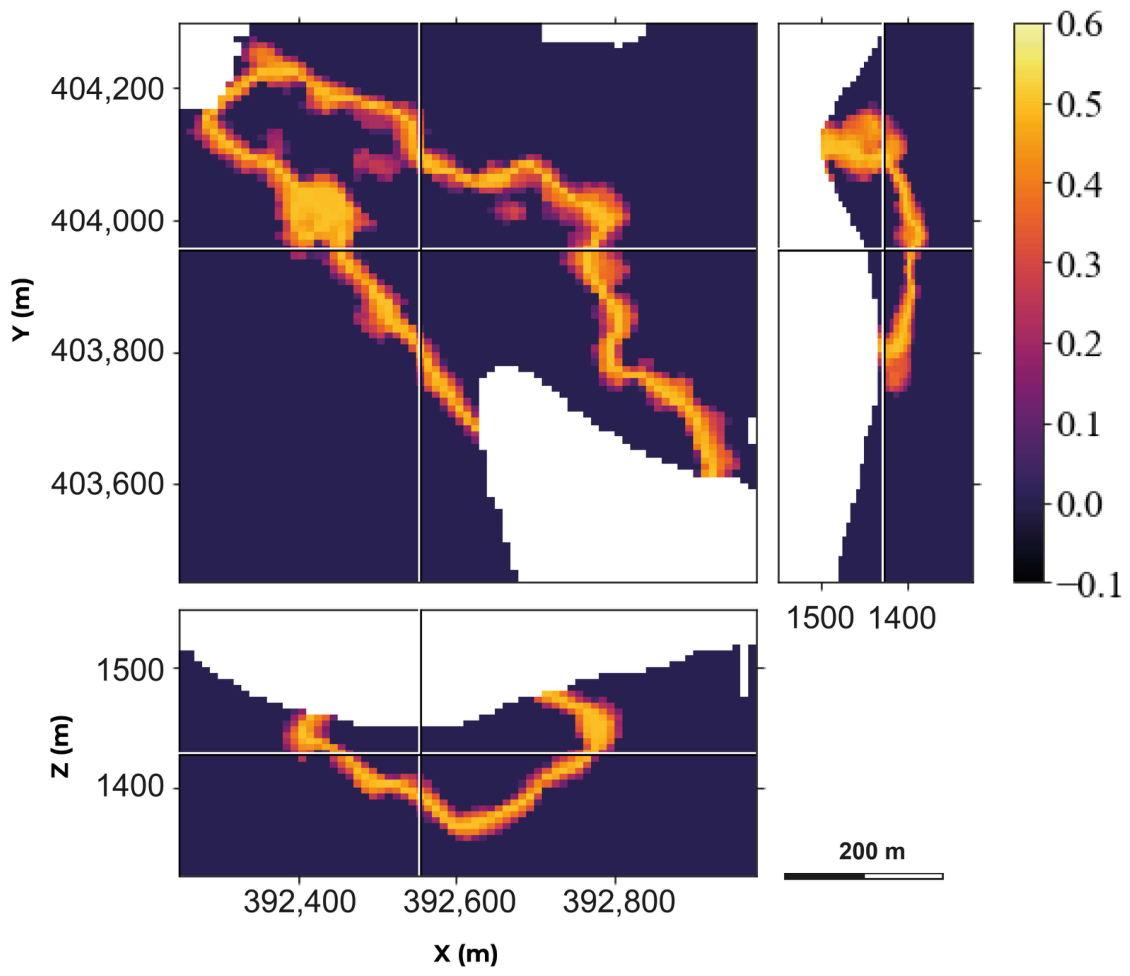
The 10,000 models enable the quantification of the uncertainty of the geometry. Figure 12 displays the standard deviation of the modeled intrusion–host rock interface across all MCMC realizations. Regions near conditioning data, drillholes, and mapped outcrop contacts show very low standard deviations, indicating high confidence in the geometry. In contrast, areas with sparse or no direct data exhibit higher standard deviation values. Notably, the uncertainty is greatest along the deeper portions of the intrusion’s boundary, reflecting variability in how far the intrusion might extend at depth.

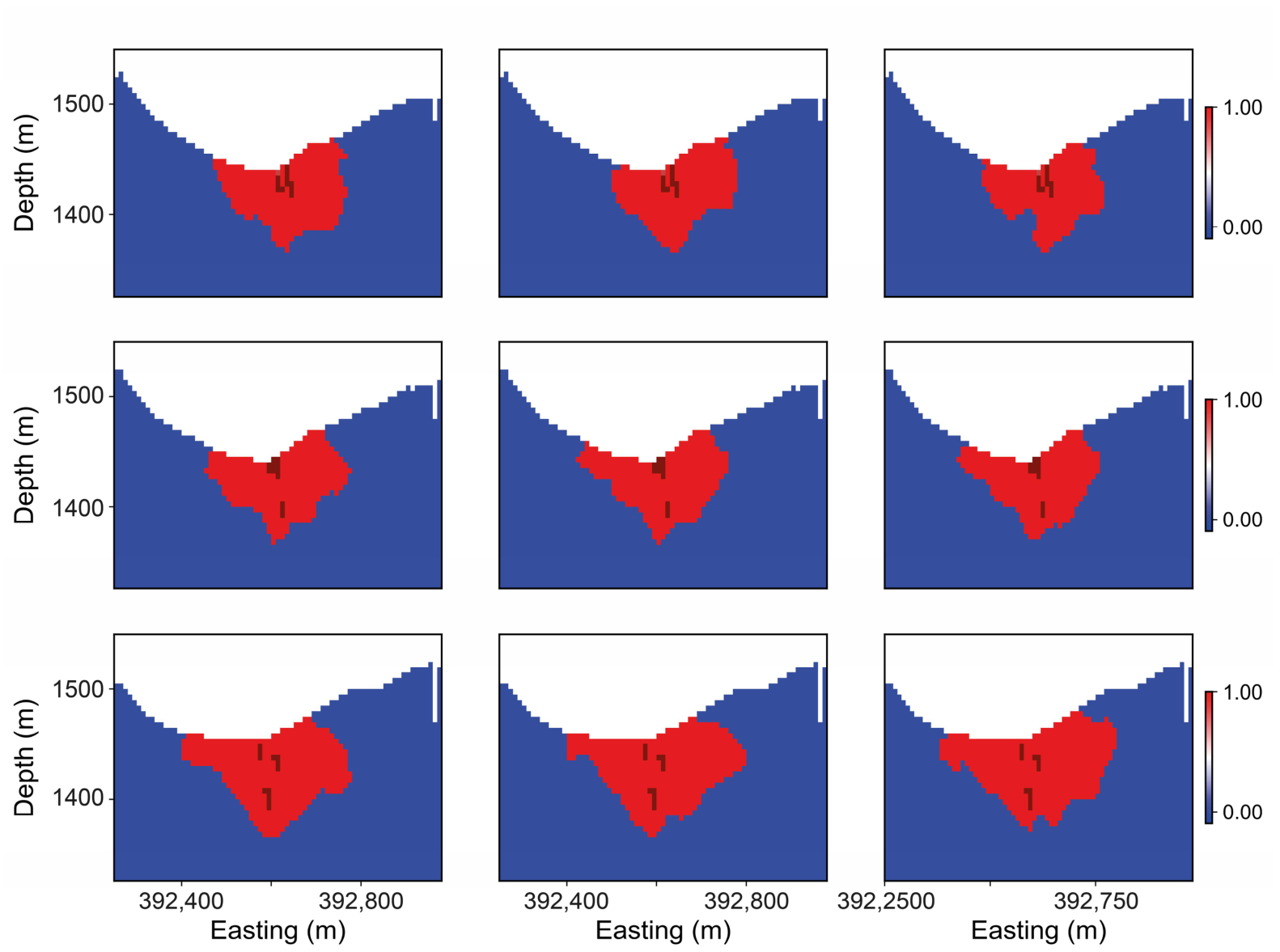
To assess the depth of the intrusion, Figure 13 presents nine posterior realizations of the intrusion geometry across three vertical cross-sections oriented along the Y-direction (slices 45, 47, and 52). Each row corresponds to a different Y-slice, and each panel within a row shows a distinct MCMC sample conditioned on the same borehole and sketch data. The red regions represent the modeled intrusive body, and the blue areas denote the host rock. Rather than enforcing the intrusion to intersect the borehole during sampling, realizations are retrospectively evaluated for consistency with borehole observations. This approach enables flexible posterior exploration while ensuring geological plausibility where intrusive material is expected beneath the borehole. The absence of topological artifacts such as disjoint volumes confirms that the signed distance function and Gaussian perturbations effectively regularize deformation [43,44]. At the same time, the Procrustes-aligned 2D sketch prior [45] provides shape guidance without imposing strict geometric templates.

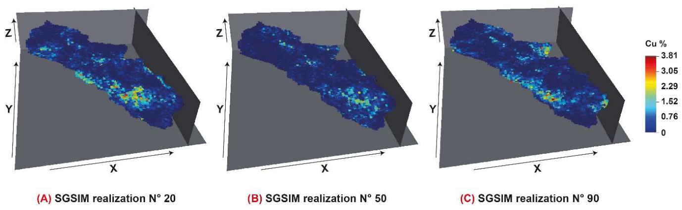
The second major component of uncertainty in this study is the spatial variability of copper grade within the modeled intrusion. As defined in the methodology, copper grade is treated as a continuous random field Z(x), modeled over the 3D volume, and assumed to follow a second-order stationary Gaussian distribution conditioned to drillhole assay data. The normal-score transform was applied to Cu grades, and the spatial variogram of Cu was modeled with three structural directions, each with a spherical model and a shared nugget effect of 0.14. The primary direction of continuity, representing the dominant trend of copper mineralization along the dip plane, has an azimuth of 136°, a range of 150–250 m, and a sill of 0.7–0.9. The secondary direction, orthogonal to the primary on the dip plane and representing minor continuity, has an azimuth of 27°, a range of 40–80 m, and a sill of 0.7–0.9. The tertiary direction, perpendicular to the dip plane and representing the shortest spatial continuity, has an azimuth of 50°, a range of 20–35 m, and a sill of 0.7–0.9. We use Sequential Gaussian Simulation (SGSIM) to generate realizations of the grade within the intrusion geometry sampled by the level-set MCMC framework. SGSIM belongs to the class of probabilistic geostatistical techniques, as described by [54]), which aim to reproduce both the statistical distribution and the spatial continuity of the underlying variable. Unlike deterministic approaches like kriging, which yield a single best estimate, SGSIM captures the full distribution of plausible outcomes [4]. Each realization honors the same conditioning data and statistical parameters but expresses a different plausible spatial configuration, making them suitable for uncertainty analysis and risk-based decision-making. As emphasized by [7], this stochastic perspective is essential in modern resource evaluation: while kriged estimates may provide local accuracy, they fail to reflect the variability and potential downside risks relevant for economic planning. Figure 14 shows three representative realizations of the copper grade, SGSIM realizations No. 20, 50, and 90 (Figure 14). To preserve the vertical resolution of the original data and avoid artificial smoothing, SGS was performed on a 5 × 5 × 1 m grid, with the vertical discretization matching the 1 m drill-core composite length, consistent with geostatistical recommendations that simulation support should not exceed the data support in the direction of highest variability [54].

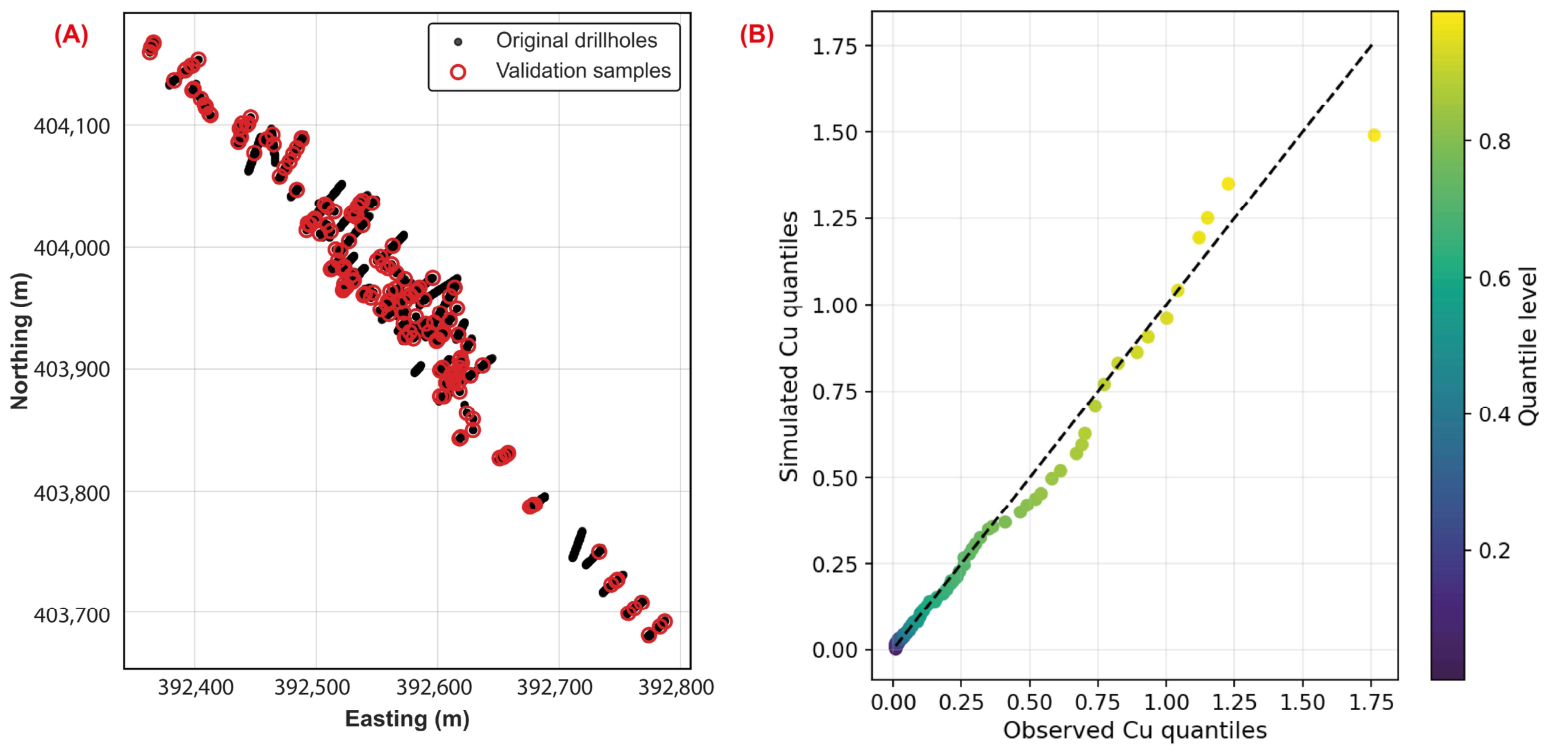
The reliability of the grade simulation is assessed through a validation analysis (Figure 15). A set of 200 validation points, withheld from the conditioning dataset prior to simulation, was used to evaluate the model, selected to reflect both the spatial distribution and grade variability of the original dataset. (Figure 15A). The quantile–quantile (Q–Q) comparison (Figure 15B) shows strong agreement between observed and simulated copper grades across most of the distribution. Minor deviations at higher quantiles indicate slight smoothing of extreme values, which is expected in Gaussian-based simulation approaches. Such sequential modeling approaches directly address the concern raised by [5] that conventional workflows often overlook the compounding effect of uncertain geology on grade-based outcomes.

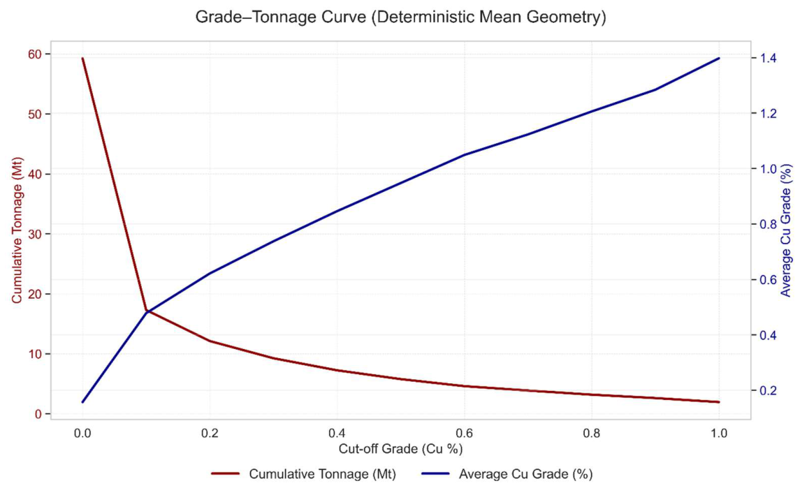
The uncertainty in orebody geometry is highlighted by comparing the deterministic mean geometry to individual MCMC realizations (Figure 16). The mean model is constructed by averaging the signed distance functions across accepted MCMC samples. This spatial averaging fills in regions that are present in any realization, effectively merging alternative geometries into a single smoothed envelope. As a result, the mean model contains 42,188 intrusive blocks, corresponding to a volume of 21.09 Mm³ and a tonnage of 59.27 Mt. In contrast, individual MCMC realizations exhibit perturbed boundaries that may extend or contract in different directions, reflecting plausible geological variability. Across the stochastic ensemble, the mean intrusion tonnage is 36.13 Mt, with a P5–P95 range of 34.19–38.31 Mt. The deterministic mean model therefore exceeds the median (P50) realization by 62.8% and lies well above the P95 envelope, demonstrating a substantial and systematic overestimation. Importantly, the realizations show relatively low dispersion (standard deviation = 1.40 Mt; CV = 3.87%), indicating that this discrepancy is not driven by stochastic noise but by geometric smoothing inherent in the mean model. These results quantitatively confirm that averaging geometry inflates tonnage estimates and masks the range of plausible orebody shapes.

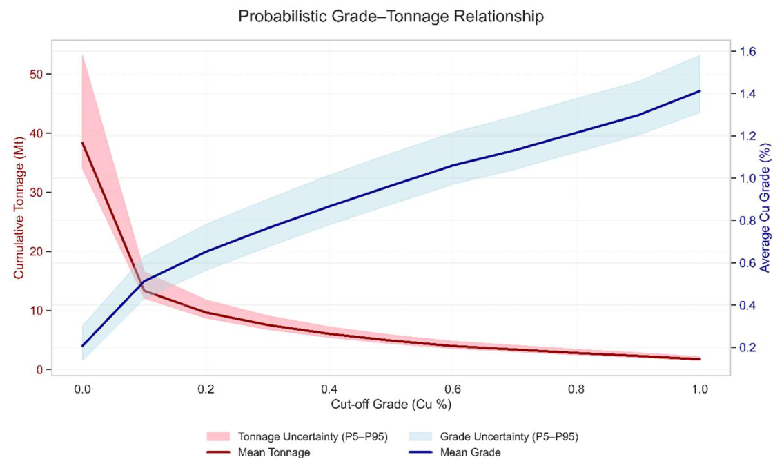
Figure 16 and Figure 17 illustrate the difference between deterministic and probabilistic interpretations of grade–tonnage relationships. In the deterministic case (Figure 16), all quantities are derived from the mean geometry combined with a single grade realization. Cumulative tonnage decreases smoothly as the cut-off grade increases, and the average copper grade increases monotonically. Because only one model is considered, this representation suggests a single, well-defined relationship between cut-off grade and economic outcome, with no indication of uncertainty.

By contrast, the grade–tonnage relationships obtained from the joint geometry–grade ensemble (Figure 17) explicitly account for uncertainty. The shaded envelopes represent P5–P95 ranges for tonnage and grade across stochastic realizations. At low cut-off grades (≤0.2% Cu), the uncertainty in cumulative tonnage is particularly large, reflecting sensitivity to geometric variability in the intrusion volume. Although the stochastic realizations show relatively limited dispersion in total tonnage (CV ≈ 3.9%), the deterministic curve consistently lies near or above the upper bound of the uncertainty envelope. This indicates that the deterministic model does not correspond to a central or representative outcome but rather reflects an upper-biased scenario caused by smoothing across alternative geometries.

4. Conclusions

This study presented a framework for sequential uncertainty quantification in mineral resource modeling by integrating stochastic geometry and grade simulation. Orebody geometry was represented as a level-set function and sampled within a Markov Chain Monte Carlo scheme. At the same time, copper grades were simulated conditionally within accepted realizations using Sequential Gaussian Simulation. This coupling ensured that grade outcomes incorporated uncertainty in orebody extent and geometry, rather than being conditioned on a single deterministic boundary.

The results show that the ensemble of level-set realizations captures spatial uncertainty in intrusion geometry, and that this structural uncertainty propagates directly into grade–tonnage estimates. The family of grade–tonnage curves obtained reflects a probabilistic range of possible outcomes: convergence occurs at low cut-off grades, while divergence at higher thresholds illustrates the variability in recoverable tonnage. This demonstrates that separating geometry and grade uncertainty underestimates risk in resource evaluation.

Uncertainty in mineral resource modeling can be considered in three interconnected components: grade variability, volumetric/structural uncertainty, and data uncertainty. The first two were addressed by sequentially simulating geometry and then grades. Third, data uncertainty, including sampling errors and assay precision, remains an essential factor that can significantly influence uncertainty quantification and resource classification. A comprehensive framework should integrate all three components, ensuring that both geological knowledge and data quality are jointly reflected in probabilistic resource estimates.

The proposed approach provides a systematic means of sequentially quantifying geological and grade uncertainty while maintaining geological plausibility. Applied to the Anti-Atlas copper intrusion, it yielded uncertainty ranges for orebody geometry and grade–tonnage relationships that are directly applicable to exploration targeting and mine planning.

References

1. Camus, J.P. Management of Mineral Resources: Creating Value in the Mining Business; SME: Littleton, CO, USA, 2002. [Google Scholar]
2. Lindi, O.T.; Aladejare, A.E.; Ozoji, T.M.; Ranta, J.P. Uncertainty Quantification in Mineral Resource Estimation. Nat. Resour. Res. 2024, 33, 2503–2526. [Google Scholar] [CrossRef] [Scilit]
3. Caers, J. Modeling Uncertainty in the Earth Sciences; John Wiley & Sons: Hoboken, NJ, USA, 2011. [Google Scholar]
4. Chiles, J.-P.; Delfiner, P. Geostatistics: Modeling Spatial Uncertainty; John Wiley & Sons: Hoboken, NJ, USA, 2012. [Google Scholar]
5. Rossi, M.E.; Deutsch, C.V. Mineral Resource Estimation; Springer: Dordrecht, The Netherlands, 2014. [Google Scholar]
6. Journel, A.G.; Isaaks, E.H. Conditional Indicator Simulation: Application to a Saskatchewan Uranium Deposit. J. Int. Assoc. Math. Geol. 1984, 16, 685–718. [Google Scholar] [CrossRef] [Scilit]
7. Deutsch, C.V. The Place of Geostatistical Simulation through the Life Cycle of a Mineral Deposit. Minerals 2023, 13, 1400. [Google Scholar] [CrossRef] [Scilit]
8. Goovaerts, P. Geostatistics for Natural Resources Evaluation; Oxford University Press: Oxford, UK, 1997. [Google Scholar]
9. Li, S.; Knights, P.; Dunn, D. Geological Uncertainty and Risk: Implications for the Viability of Mining Projects. J. Coal Sci. Eng. 2008, 14, 176–180. [Google Scholar] [CrossRef] [Scilit]
10. Dominy, S.C.; Edgar, W.B. Approaches to Reporting Grade Uncertainty in High Nugget Gold Veins. Appl. Earth Sci. 2012, 121, 29–42. [Google Scholar] [CrossRef] [Scilit]
11. McManus, S.; Rahman, A.; Coombes, J.; Horta, A. Comparison of Interpretation Uncertainty in Spatial Domains Using Portable X-Ray Fluorescence and ICP Data. Appl. Comput. Geosci. 2021, 12, 100067. [Google Scholar] [CrossRef] [Scilit]
12. Jordão, H.; Sousa, A.J.; Soares, A. Using Bayesian Neural Networks for Uncertainty Assessment of Ore Type Boundaries in Complex Geological Models. Nat. Resour. Res. 2023, 32, 2495–2514. [Google Scholar] [CrossRef] [Scilit]
13. Journel, A.G.; Huijbregts, C.J. Mining Geostatistics; Breau De RecherchesGeologiques Et Miners, France Academic Pres Harcout Brace & Company, Publishers: London, UK; San Diego, CA, USA; New York, NY, USA; Boston, MA, USA; Sidney, Australia; Toronto, ON, Canada, 1978. [Google Scholar]
14. Deutsch, C.V.; Journel, A.G. GSLIB: Geostatistical Software Library; Oxford University Press: New York, NY, USA, 1998. [Google Scholar]
15. Pyrcz, M.J.; Deutsch, C.V. Geostatistical Reservoir Modeling; Oxford University Press: New York, NY, USA, 2014. [Google Scholar]
16. Dowd, P.A. Risk Assessment in Reserve Estimation and Open-Pit Planning. Trans. Inst. Min. Metall. (Sect. A Min. Ind.) 1994, 103, A148. [Google Scholar]
17. Smith, M.; Dimitrakopoulos, R. The Influence of Deposit Uncertainty on Mine Production Scheduling. Int. J. Surf. Min. Reclam. Environ. 1999, 13, 173–178. [Google Scholar] [CrossRef] [Scilit]
18. Emery, X. Two Ordinary Kriging Approaches to Predicting Block Grade Distributions. Math. Geol. 2006, 38, 801–819. [Google Scholar] [CrossRef] [Scilit]
19. Ortiz, J.M.; Emery, X. Geostatistical Estimation of Mineral Resources with Soft Geological Boundaries: A Comparative Study. J. S. Afr. Inst. Min. Metall. 2006, 106, 577. [Google Scholar]
20. Dimitrakopoulos, R. Conditional Simulation Algorithms for Modelling Orebody Uncertainty in Open Pit Optimisation. Int. J. Surf. Min. Reclam. Environ. 1998, 12, 173–179. [Google Scholar] [CrossRef] [Scilit]
21. Bastante, F.G.; Ordóñez, C.; Taboada, J.; Matías, J.M. Comparison of Indicator Kriging, Conditional Indicator Simulation and Multiple-Point Statistics Used to Model Slate Deposits. Eng. Geol. 2008, 98, 50–59. [Google Scholar] [CrossRef] [Scilit]
22. Sojdehee, M.; Rasa, I.; Nezafati, N.; Abedini, M.V.; Madani, N.; Zeinedini, E. Probabilistic Modeling of Mineralized Zones in Daralu Copper Deposit (SE Iran) Using Sequential Indicator Simulation. Arab. J. Geosci. 2015, 8, 8449–8459. [Google Scholar] [CrossRef] [Scilit]
23. Emery, X. Simulation of Geological Domains Using the Plurigaussian Model: New Developments and Computer Programs. Comput. Geosci. 2007, 33, 1189–1201. [Google Scholar] [CrossRef] [Scilit]
24. Beucher, H.; Galli, A.; Le Loc’h, G.; Ravenne, C. Including a Regional Trend in Reservoir Modelling Using the Truncated Gaussian Method. In Geostatistics Tróia’92; Soares, A., Ed.; Springer: Dordrecht, The Netherlands, 1993. [Google Scholar]
25. Yunsel, T.Y.; Ersoy, A. Geological Modeling of Rock Type Domains in the Balya (Turkey) Lead-Zinc Deposit Using Plurigaussian Simulation. Cent. Eur. J. Geosci. 2013, 5, 77–89. [Google Scholar] [CrossRef] [Scilit]
26. Yunsel, T.Y.; Ersoy, A. Geological Modeling of Gold Deposit Based on Grade Domaining Using Plurigaussian Simulation Technique. Nat. Resour. Res. 2011, 20, 231–249. [Google Scholar] [CrossRef] [Scilit]
27. Rondon, O. A Look at Plurigaussian Simulation for a Nickel Laterite Deposit. In Proceedings of the 7th International Mining & Geology Conference; The Australasian Institute of Mining and Metallurgy: Melbourne, Australia, 2009. [Google Scholar]
28. Deraisme, J.; Field, M. Geostatistical Simulations of Kimberlite Orebodies and Application to Sampling Optimisation. In Proceedings of the 6th International Mining Geology Conference; Australasian Institute of Mining and Metallurgy: Melbourne, VIC, Australia, 2006; pp. 193–203. [Google Scholar]
29. Betzhold, J.; Roth, C. Characterizing the Mineralogical Variability of a Chilean Copper Deposit Using Plurigaussian Simulations. J. S. Afr. Inst. Min. Metall. 2000, 100, 111–119. [Google Scholar]
30. Skvortsova, T.; Beucher, H.; Armstrong, M.; Forkes, J.; Thwaites, A.; Turner, R. Simulating the Geometry of a Granite-Hosted Uranium Orebody. In Geostatistics Rio 2000; Armstrong, M., Bettini, C., Champigny, N., Galli, A., Remacre, A., Eds.; Kluwer Academic: Dordrecht, The Netherlands, 2002. [Google Scholar]
31. Armstrong, M.; Galli, A.; Le-Loch, G.; Geffroy, F.; Eschard, R. Plurigaussian Simulations in Geosciences; Springer: Berlin, Germany, 2003. [Google Scholar]
32. Riquelme, R.; Le Loc’h, G.; Carrasco, P. Truncated Gaussian and Plurigaussian Simulations of Lithological Units in Mansa Mina Deposit. In Proceedings of the 8th International Geostatistics Congress; Ortiz, J.M., Emery, X., Eds.; Gecamin Ltda: Santiago, Chile, 2008. [Google Scholar]
33. Chatterjee, S.; Dimitrakopoulos, R.; Mustapha, H. Dimensional Reduction of Pattern-Based Simulation Using Wavelet Analysis. Math. Geosci. 2012, 44, 343–374. [Google Scholar] [CrossRef] [Scilit]
34. Guardiano, F.B.; Srivastava, R.M. Multivariate Geostatistics: Beyond Bivariate Moments. In Geostatistics Tróia’92; Soares, A., Ed.; Springer: Dordrecht, The Netherlands, 1993. [Google Scholar]
35. Arpat, G.B.; Caers, J. Conditional Simulation with Patterns. Math. Geol. 2007, 39, 177–203. [Google Scholar] [CrossRef] [Scilit]
36. Mariethoz, G.; Caers, J. Multiple-Point Geostatistics: Stochastic Modeling with Training Images; John Wiley & Sons: Hoboken, NJ, USA, 2014. [Google Scholar]
37. Osterholt, V.; Dimitrakopoulos, R. Simulation of Wireframes and Geometric Features with Multiple-Point Techniques: Application at Yandi Iron Ore Deposit. Strateg. Mine Plan. AusIMM Spectr. Ser. 2007, 14, 95–124. [Google Scholar]
38. Dimitrakopoulos, R.; Farrelly, C.T.; Godoy, M. Moving Forward from Traditional Optimization: Grade Uncertainty and Risk Effects in Open-Pit Design. Min. Technol. 2002, 111, 82–88. [Google Scholar] [CrossRef] [Scilit]
39. Wilde, B.J.; Deutsch, C.V. Kriging and Simulation in Presence of Stationary Domains: Developments in Boundary Modeling. In Geostatistics Oslo 2012; Abrahamsen, P., Hauge, R., Kolbjørnsen, O., Eds.; Springer: Dordrecht, The Netherlands, 2012. [Google Scholar]
40. Maleki, M.; Emery, X. Joint Simulation of Grade and Rock Type in a Stratabound Copper Deposit. Math. Geosci. 2015, 47, 471–495. [Google Scholar] [CrossRef] [Scilit]
41. Hosseini, S.A.; Asghari, O.; Emery, X. Direct Block-Support Simulation of Grades in Multi-Element Deposits: Application to Recoverable Mineral Resource Estimation at Sungun Porphyry Copper-Molybdenum Deposit. J. South. Afr. Inst. Min. Metall. 2017, 117, 577–585. [Google Scholar] [CrossRef] [Scilit]
42. Sadeghi, B.; Madani, N.; Carranza, E.J.M. Combination of Geostatistical Simulation and Fractal Modeling for Mineral Resource Classification. J. Geochem. Explor. 2015, 149, 59–73. [Google Scholar] [CrossRef] [Scilit]
43. Fouedjio, F.; Scheidt, C.; Yang, L.; Achtziger-Zupančič, P.; Caers, J. A Geostatistical Implicit Modeling Framework for Uncertainty Quantification of 3D Geo-Domain Boundaries: Application to Lithological Domains from a Porphyry Copper Deposit. Comput. Geosci. 2021, 157, 104931. [Google Scholar] [CrossRef] [Scilit]
44. Wang, L.; Peeters, L.; MacKie, E.J.; Yin, Z.; Caers, J. Unraveling the Uncertainty of Geological Interfaces through Data-Knowledge-Driven Trend Surface Analysis. Comput. Geosci. 2023, 178, 105419. [Google Scholar] [CrossRef] [Scilit]
45. Wei, X.; Yin, Z.; Bonner, W.; Caers, J. Knowledge-Driven Stochastic Modeling of Geological Geometry Features Conditioned on Drillholes and Outcrop Contacts. Comput. Geosci. 2025, 196, 105779. [Google Scholar] [CrossRef] [Scilit]
46. Sterk, R.; de Jong, K.; Partington, G.; Kerkvliet, S.; van de Ven, M. Domaining in Mineral Resource Estimation: A Stock-Take of 2019 Com-Mon Practice 2019. Available online: https://www.researchgate.net/publication/350567948_Domaining_in_Mineral_Resource_Estimation_A_Stock-Take_of_2019_Common_Practice (accessed on 2 July 2026).
47. Yang, L.; Achtziger-Zupančič, P.; Caers, J. 3D Modeling of Large-Scale Geological Structures by Linear Combinations of Implicit Functions: Application to a Large Banded Iron Formation. Nat. Resour. Res. 2021, 30, 3139–3163. [Google Scholar] [CrossRef] [Scilit]
48. Gower, J.C. Generalized Procrustes Analysis. Psychometrika 1975, 40, 33–51. [Google Scholar] [CrossRef] [Scilit]
49. Goodall, C. Procrustes Methods in the Statistical Analysis of Shape. J. R. Stat. Soc. Ser. B (Methodol.) 1991, 53, 285–321. [Google Scholar] [CrossRef] [Scilit]
50. Hastings, W.K. Monte Carlo Sampling Methods Using Markov Chains and Their Applications; Oxford University Press: Oxford, UK, 1970. [Google Scholar]
51. Metropolis, N.; Rosenbluth, A.W.; Rosenbluth, M.N.; Teller, A.H.; Teller, E. Equation of State Calculations by Fast Computing Machines. J. Chem. Phys. 1953, 21, 1087–1092. [Google Scholar] [CrossRef] [Scilit]
52. Pakyuz-Charrier, E.; Giraud, J.; Ogarko, V.; Lindsay, M.; Jessell, M. Drillhole Uncertainty Propagation for Three-Dimensional Geological Modeling Using Monte Carlo. Tectonophysics 2018, 747, 16–39. [Google Scholar] [CrossRef] [Scilit]
53. Bouskri, I.; Ilmen, S.; Souhassou, M.; Ikenne, M.; Zoheir, B.; Hajjar, Z.; Maacha, L.; Benzougagh, B.; Kader, S.; Jabbour, M.; et al. Geological Setting, Mineralogy, and Isotopic Characterization of the Jbel N’Zourk Copper Deposit, Central Anti-Atlas, Morocco. Ore Geol. Rev. 2025, 179, 106533. [Google Scholar] [CrossRef] [Scilit]
54. Journel, A.G.; Huijbregts, C.J. Mining Geostatistics; Academic Press: London, UK, 1978. [Google Scholar]
Figure 1. A generic schematic illustrating the mechanics of the level-set perturbation method. (A) Initial signed distance field n ; (B) sampled Gaussian velocity field v ; (C) extended velocity field f ; (D) updated field n + 1 with perturbed (red) and original (dashed) interfaces. (E,F) 3D example of the corresponding deformation from n to n + 1 . Adapted from [44].
Minerals 16 00804 g001
Figure 2. (A) Categorical encoding of drillholes, outcrops, and topography in the 3D model. Red, blue, and green points represent intrusion (1), non-intrusion (0), and contact (0.5), respectively. (B) A binary representation of the deposit (red) and non-deposit region (blue).
Minerals 16 00804 g002
Figure 3. Sketch falsification results. Three candidate sketches (AC) evaluated against drillhole lithological data (black bars). Thin blue lines show individual MCMC realizations; the solid blue line is the median boundary (P50); dashed lines and shading mark the 5–95% uncertainty band; the red contour is the candidate sketch geometry.
Minerals 16 00804 g003
Figure 4. Variogram range falsification posterior geometry ensembles. Upper panels (AD): posterior geometry ensembles for Range 1 (blue), Range 2 (orange), Range 3 (green), and Range 4 (purple), showing the median boundary (solid line, P50) and 5–95% uncertainty envelope (shaded). Lower panels (EH): corresponding exponential variogram envelopes bounded by the short and long range limits, with the used range marked by the red dashed vertical line.
Minerals 16 00804 g004
Figure 5. Variogram range falsification, curvature distributions. Posterior distributions of mean absolute interface curvature |κ| for each range configuration. The red vertical line marks the sketch reference value ksketch = 0.0477. The orange dashed vertical lines mark the 99% confidence interval boundaries of the Range 2 posterior curvature distribution
Minerals 16 00804 g005
Figure 6. (A) Initial model (black) and accepted sketch (blue) on the 70 × 50 grid. Remaining panels: posterior ensembles for the 4-drillhole (B), 5-drillhole (C), and 6-drillhole (D) scenarios. Thin blue lines show individual MCMC realizations; the red contour is the reference geometry; black bars show drillhole traces with bold segments at boundary intersections.
Minerals 16 00804 g006
Figure 7. Total loss as a function of sampling steps for the 4-drillhole (dark blue), 5-drillhole (olive), and 6-drillhole (pink) scenarios on a logarithmic scale. All three chains stabilise within 300–500 iterations. The higher stationary loss of the 6-drillhole scenario reflects the additional data constraints imposed by the denser observation set.
Minerals 16 00804 g007
Figure 8. Schematic cross-sections of the Jbel N’Zourk area (modified after [53]) showing structural control on copper mineralization. (A) Regional section illustrating stratiform-style copper occurrences broadly following layered dolomites and siltstones. (B) Detailed section across the Jbel N’Zourk fault, where deformation reworked earlier mineralization and focused on hydrothermal fluids along fractures and shear zones, producing copper enrichment across multiple lithologies. This setting is used here as an analogue for the Tarmante deposit, where mineralization is likewise structurally localized within shear zones rather than strictly stratigraphic. Green dot: outcrop point.
Minerals 16 00804 g008
Figure 9. Model realizations during the burn-in stage (A) iteration 0, (B) iteration 500, (C) 1000, (D) 2000. Purple blocks represent the modeled intrusion; black squares mark drillhole intervals, with grey dots at the drillhole collar points. Green dots denote surface outcrops and blue dots the topographic surface.
Minerals 16 00804 g009
Figure 10. (A) Evolution of the loss-function components during 10,000 MCMC sampling steps. The total loss (blue) combines contributions from borehole constraints (orange), surface outcrop constraints (green), and sketch-based structural constraints (red). The rapid decrease followed by stabilization of all components indicates convergence toward a stationary regime. (B) Trace plot of intrusion volume (voxel count) as a function of sampling steps. The red dashed line marks the burn-in period (≈2000 iterations). After burn-in, intrusion volume fluctuates within a stable range, indicating that the Markov chain has reached stationarity and is exploring geometrical variability. (C) Empirical autocorrelation function p(t) of the total loss, computed from the post-burn-in chain.
Minerals 16 00804 g010
Figure 11. Model realization after convergence (A) 9400 (B) 9600 (C) 9800 (D) 10,000. Purple blocks represent the modeled intrusion; black squares mark drillhole intervals, with grey dots at the drillhole collar points. Green dots denote surface outcrops and blue dots the topographic surface.
Minerals 16 00804 g011
Figure 12. Three orthogonal slices through the standard deviation field of the posterior intrusion geometry obtained from the MCMC ensemble. The slices intersect at a fixed (x, y, z) location within the 3D domain. The color scale represents spatial uncertainty (standard deviation of the level-set function).
Minerals 16 00804 g012
Figure 13. Geological model realizations displayed as vertical cross-sections along the Y-direction at slice indices 45 (top row), 47 (middle row), and 52 (bottom row). Each panel shows a different MCMC sample with inferred geometry, overlaid with borehole constraints. High-contrast binary colors distinguish intrusion (red) from the non-intrusion (blue).
Minerals 16 00804 g013
Figure 14. Selected realizations from Sequential Gaussian Simulation (SGSIM) illustrating spatial variability in copper (Cu) grade distribution across the deposit. Panels (AC) correspond to realizations number 20, 50, and 90, respectively.
Minerals 16 00804 g014
Figure 15. Validation of copper grade simulation. (A) Spatial distribution of original drillhole samples (black) and validation samples (red), illustrating the data coverage used for conditional simulation. (B) Quantile–quantile (Q–Q) plot comparing observed and simulated copper grades.
Minerals 16 00804 g015
Figure 16. Deterministic grade–tonnage relationship derived from the mean geometry model, obtained by averaging posterior level-set realizations. Cumulative tonnage (red axis) and average copper grade (blue axis) are shown as functions of cut-off grade.
Minerals 16 00804 g016
Figure 17. Combined grade–tonnage curves with uncertainty envelopes derived from a set of stochastic realizations. The plot shows how cumulative tonnage (red), average copper grade (blue), Shaded areas represent the P5–P95 percentile ranges for each variable.
Minerals 16 00804 g017