
Article

Probabilistic Modeling of Lateritic Nickel Mineral Resources

1
Geovariances, 77210 Avon, France
2
Vale Indonesia, Jakarta 12190, Indonesia
*
Author to whom correspondence should be addressed.
Minerals 2026, 16(5), 551; https://doi.org/10.3390/min16050551
Submission received: 31 December 2025 / Revised: 5 April 2026 / Accepted: 1 May 2026 / Published: 20 May 2026
(This article belongs to the Special Issue Geostatistical Methods and Practices for Specific Ore Deposits)

Abstract

Lateritic nickel deposits exhibit complex weathering-driven geometries, strong vertical variability, and complex multivariate geochemical relationships. These characteristics challenge conventional deterministic resource modeling. This paper presents a unified probabilistic workflow for lateritic nickel mineral resource modeling that integrates lithology and grade simulation within a consistent geostatistical framework. The methodology combines unfolding, plurigaussian simulation, multivariate imputation of incomplete datasets, projection pursuit multivariate transformation (PPMT) for decorrelation, and conditional simulation using the Turning Bands algorithm. Application to an Indonesian lateritic nickel deposit demonstrates reproduction of lithological proportions, spatial continuity, marginal distributions, and complex multivariate relationships. The proposed workflow enables explicit quantification of geological and grade uncertainty, providing a basis for uncertainty assessment in recoverable resource estimation and supporting downstream applications such as resource classification and drillhole spacing analysis.

1. Introduction

Modeling lateritic nickel deposits presents several challenges. First, mineralization continuity frequently departs from simple planar geometries along strike and dip as a consequence of weathering processes. Second, these deposits commonly exhibit pronounced vertical variability. Downhole profiles often include transitional zones in which lithologies alternate over short distances, complicating the delineation of sharp contacts and the reliable modeling of layer thicknesses. Third, the geochemical variables of interest exhibit complex multivariate relationships and are frequently subject to compositional constraints.
In addition to these geological and statistical complexities, natural geological phenomena are inherently uncertain. Geological heterogeneity, combined with the limited and spatially sparse information provided by drillhole data, implies that uncertainty is an intrinsic component of mineral resource evaluation and cannot be eliminated, only quantified and managed. Traditional deterministic approaches often underrepresent this uncertainty, potentially leading to biased resource estimates and an incomplete assessment of associated risks [1].
A typical probabilistic modeling workflow relies on conditional simulation to generate multiple equiprobable realizations of geological domains and grade variables [1]. The specific implementation depends on the characteristics of the deposit and may require different simulation techniques, along with appropriate pre- and post-processing steps.
The objective of this paper is to apply and evaluate an integrated workflow for the probabilistic modeling of lateritic nickel resources, combining established geostatistical techniques. The workflow comprises unfolding, missing data imputation, ratio transformation (if required), multigaussian transformation, simulation of categorical variables followed by simulation of continuous variables, and finally recoverable resource calculation accounting for inherent uncertainty. The overall workflow is outlined in Figure 1.
This study is presented as a case study to evaluate the application of this workflow and its implications for resource estimation under uncertainty.
The remainder of the paper is organized as follows. The next section presents related work on the modeling of lateritic nickel deposits. This is followed by a detailed literature review describing the geostatistical methods incorporated in the workflow. Finally, a case study illustrates the application of the methodology to a lateritic nickel deposit located in Indonesia.

2. Related Work

Several authors have investigated methodological frameworks to address the challenges associated with mineral resource estimation and classification in lateritic nickel deposits.
Conoras and Lamburu [2] compared nickel grade estimation and resource classification obtained using ordinary kriging (OK) and sequential Gaussian simulation (SGS), highlighting the impact of stochastic modeling on classification outcomes.
Addressing the structural complexity of lateritic profiles, Richmond [3] demonstrated that conditional simulations performed in an unfolded stratigraphic framework produce more geologically realistic results than simulations conducted in a conventional Cartesian coordinate system.
Lithological uncertainty has also been explicitly modeled. Toro et al. [4] applied sequential indicator simulation (SIS) to represent the spatial variability of lithological horizons within a lateritic nickel deposit. Similarly, Dagasan et al. [5] investigated the use of multiple-point statistics (MPS) to model complex geological contact geometries, albeit in the context of a lateritic bauxite deposit.
Multivariate simulation at selective mining unit (SMU) support has been explored by several authors. Deraisme et al. [6] implemented direct block co-simulation of five correlated variables and proposed a scenario reduction strategy to select representative realizations for downstream risk assessment. In a related approach, de Freitas Silva and Dimitrakopoulos [7] introduced a regolith “unwrinkling” methodology in which weathering profiles are geometrically flattened prior to simulation. Thicknesses are simulated first, followed by multivariate direct block co-simulation using minimum/maximum autocorrelation factors (MAF) to preserve cross-correlation structures.
Uncertainty associated with drilling density has also been investigated. Neves et al. [8] applied sequential indicator simulation (SIS) and SGS to jointly simulate thickness, nickel grade, and ore type. They subsequently performed virtual sampling of realizations and re-simulated the variables to quantify the uncertainty induced by drillhole spacing.
For resource classification, Isatelle and Rivoirard [9] compared conditional simulation with the specific areas method in a lateritic nickel context, while Renaldy et al. [10] extended this comparison to the Halmahera deposit in Indonesia.
Although previous studies have addressed individual components of probabilistic modeling, such as lithological simulation, multivariate grade co-simulation, stratigraphic unfolding, and resource classification methodologies, fewer studies have documented the integration of these components within a single consistent workflow applied to lateritic nickel deposits.

3. Literature Review

3.1. Unfolding

In stratigraphic settings where geological units have been subjected to folding, warping, or irregular weathering processes, mineralization continuity often departs from a simple planar geometry along strike or dip. Under such conditions, conventional variography and interpolation based on linear vectors in Cartesian space may fail to adequately represent spatial continuity, as Euclidean distances do not reflect true geological connectivity.
Several methodologies have been proposed to address this limitation [3]:
  • Simple unfolding (or “unwrinkling”), in which data are transformed relative to a 2D unfolding surface [11].
  • Stratigraphic coordinate transformation, where data are mapped and scaled between two bounding stratigraphic surfaces [12].
  • Full 3D unfolding, in which data are transformed using a volumetric deformation model (e.g., tetrahedral grids) to obtain a geometrically consistent unfolded domain [13].
  • Locally varying anisotropy (LVA), also referred to as dynamic anisotropy, where data remain in Cartesian space, while search neighborhoods and variogram ellipsoids are locally reoriented to follow geological trends [14].
Among these approaches, simple unfolding, stratigraphic transformation, and full 3D unfolding are particularly suited to lateritic nickel deposits.

3.2. Pluri-Gaussian Simulation (PGS)

Methodologies for categorical variable simulation can be broadly divided into object-based and pixel-based approaches. Object-based methods are generally not well suited for lateritic nickel deposits and are more commonly applied in oil reservoir modeling.
Among pixel-based methods, the most widely used techniques are sequential indicator simulation (SIS) [15], the truncated Gaussian Simulation family (TGS) [16,17], and multiple-point statistics (MPS) methods [18,19].
All of these approaches have been applied to lateritic nickel deposits. However, truncated Gaussian simulations are particularly powerful because they allow explicit control of contact relationships through the simulation of one or several underlying continuous Gaussian fields. In this framework, geological consistency can be enforced; for example, limonite can be prevented from being in direct contact with bedrock if such a relationship is geologically implausible.
The truncated Gaussian simulation workflow can be summarized as follows:
  • Define a truncation rule describing the contact relationships between categories. For simple stratigraphic deposits, this rule can be defined in one dimension (Truncated Gaussian Simulation (TGS)), whereas more complex geological environments may require two or more dimensions (Pluri-Gaussian Simulation (PGS)).
  • Infer the variogram(s) of the underlying Gaussian variable(s) from the indicator variograms of the categorical variables [17,20].
  • Assign Gaussian values to the categorical samples in a manner consistent with the inferred variogram model, using a Gibbs sampling algorithm.
  • Simulate the Gaussian variable(s) using an appropriate Gaussian simulation algorithm.
  • Apply the truncation rule to transform the simulated Gaussian field(s) into categorical realizations. Local proportions, estimated from data or secondary variables, may be incorporated to locally adjust the truncation thresholds on a block-by-block basis while preserving the prescribed contact relationships.

3.3. Multivariate Imputation

In mineral resource projects, incomplete sampling of variables is frequent. Economic constraints, operational limitations, variations in sampling quality, technological changes in drilling practices, and evolving project objectives often lead to datasets in which not all variables are measured at every location. These heterotopic data configurations complicate multivariate geostatistical analysis, particularly when the modeling framework requires all variables to be available at the same spatial positions [21].
Various approaches have been proposed to address missing data, including single imputation (SI), maximum likelihood estimation (MLE), and multiple imputation (MI). Among these, MI is generally favored in geostatistical contexts because it generates multiple conditional realizations of the missing values that can be directly incorporated into stochastic simulation workflows [21]. The MI procedure can be summarized as follows:
  • Estimate, at a location with missing data, the prior distribution of the variable to be imputed using neighboring data of the same variable. Under the multiGaussian assumption, this corresponds to the simple kriging conditional distribution and represents the distribution of potential outcomes conditioned on spatial information.
  • Estimate the likelihood distribution conditioned on the colocated secondary variables. This conditional distribution may be obtained parametrically [22], through kernel density estimation (KDE) [22], or using Gaussian mixture models (GMM) [23], and represents the distribution of potential outcomes conditioned on multivariate relationships.
  • Combine the prior and likelihood distributions through Bayesian updating to obtain the posterior conditional distribution.
  • Generate an imputed value by stochastic sampling from the resulting posterior distribution.
Existing multivariate data imputation algorithms do not guarantee the preservation of compositional constraints.

3.4. Compositional Data

In mineral resource evaluations involving multiple assayed constituents, it is common that the variables are strictly positive and constrained by a constant sum, such as 100%, 1, or 1,000,000 (ppm). These datasets are referred to as compositional data, as they represent parts of a whole and therefore convey relative rather than absolute information. Direct application of standard statistical or geostatistical methods in Euclidean space may lead to inconsistencies, including spurious correlations and incoherent predictions that violate the closure constraint. To address this issue, Aitchison [24] introduced a formal framework in which compositions are represented in a D-dimensional simplex, a constrained sample space endowed with its own algebraic and geometric structure.
A common strategy in geostatistical applications is to map compositions from the simplex to an unconstrained Euclidean space through log-ratio transformations. After transformation, standard multivariate geostatistical tools, such as variogram modeling, kriging, or simulation, can be applied to the transformed variables. Estimations are subsequently back-transformed to recover estimates in the original compositional domain, thereby ensuring that the resulting variables remain positive and satisfy the constant-sum constraint. Several log-ratio transformations have been proposed, including the additive log-ratio (alr), centered log-ratio (clr), multiplicative log-ratio (mlr), and isometric log-ratio (ilr), each with distinct mathematical properties and implications for interpretation and modeling.
A practical limitation of log-ratio methods arises from the presence of zero values, since the logarithmic function is undefined at zero. In mining datasets, zeros may occur due to detection limits, rounding, or genuinely absent constituents. This restriction has motivated the development of alternative ratio-based transformations that avoid the direct use of logarithms, such as simple ratios and power-ratio formulations [25,26]. The primary justification for retaining the logarithmic transformation is that it often produces transformed variables with improved distributional behavior, particularly reduced skewness [25].
All of these transformation-based approaches remove the compositional constraint by operating in an unconstrained space and reimposing closure through back-transformation. Consequently, they provide a coherent framework for modeling multivariate geochemical data, including applications to lateritic nickel deposits.

3.5. Projection Pursuit Multivariate Transform (PPMT)

Classical multivariate geostatistical modeling is commonly based on the Linear Model of Coregionalization (LMC), which requires the joint modeling of all direct and cross-variograms. As the number of variables increases, the number of covariance functions that must be specified grows rapidly, rendering the approach cumbersome and often impractical in high-dimensional settings.
An alternative strategy consists of transforming the correlated variables into a set of uncorrelated factors, modeling these factors independently, and subsequently applying a back-transformation to recover the original dependence structure. Linear decorrelation techniques such as Principal Component Analysis (PCA) [27] or Min/Max Autocorrelation Factors (MAF) [28] are frequently used for this purpose. These methods diagonalize the covariance matrix and produce orthogonal factors that can be simulated independently.
However, linear transformations present important limitations. When decorrelated factors are subjected to univariate Gaussian transformation prior to simulation, correlation may be reintroduced. Furthermore, complex dependency structures, including nonlinear relationships, heteroscedasticity, and constraints, cannot be fully characterized by second-order statistics alone. Such dependencies are not eliminated by linear decorrelation [29].
These limitations motivate the use of multiGaussian transformations, whose objective is to map the original variables into a set of mutually uncorrelated factors that are jointly Gaussian. In this transformed space, the factors can be simulated independently, and the inverse transformation restores the original multivariate structure.
Several approaches have been proposed in the literature, including the Stepwise Conditional Transformation (SCT) [30], Iterative Gaussianization (IG) [31], and the Spatial Multivariate Morphing Transformation (SMMT) [32]. Among these, the Projection Pursuit Multivariate Transform (PPMT) [33,34] is one of the most widely adopted techniques in geostatistical applications.
The PPMT proceeds iteratively as follows:
  • Apply a univariate Gaussian transformation to each variable.
  • Perform a sphering transformation.
  • Identify a projection direction that maximizes deviation from Gaussianity.
  • Gaussianize the data along the selected projection.
  • Repeat steps 3 and 4 until the joint distribution converges to a multivariate Gaussian distribution with identity covariance matrix.
The back-transformation is obtained by sequentially inverting each step of the forward transformation. This requires storing the transformation parameters at each iteration.
These transformations can be combined. For example, PPMT may be integrated with MAF to account for spatial autocorrelation.
Most of these transformations require complete multivariate datasets, meaning that all variables must be available for all samples. This requirement highlights the importance of missing data imputation prior to multivariate modeling.

3.6. Turning Bands Simulation (TBS)

Several algorithms are available for the conditional simulation of Gaussian random variables. The most widely implemented in commercial geostatistical software are Sequential Gaussian Simulation (SGS) [35] and Turning Bands Simulation (TBS) [36].
SGS generates realizations sequentially along a random path, conditioning each simulated node to previously simulated values and available data. Although robust and flexible, its sequential nature can lead to significant computational burden for large grids or dense datasets.
Direct block simulation approaches [37,38,39] alleviate part of this computational demand by simulating directly at the Selective Mining Unit (SMU) support. However, these methods rely on a change-of-support model and do not explicitly reproduce sample-scale variability.
For recoverable reserve estimation, a widely accepted and theoretically consistent strategy consists of generating multiple conditional realizations at a fine scale and subsequently upscaling the realizations to the target block support by linear averaging [40].
Turning Bands Simulation offers a computationally efficient alternative to SGS. Because simulations along one-dimensional bands are independent, the method is naturally parallelizable, resulting in improved performance for large-scale problems.
The Turning Bands algorithm proceeds as follows:
  • Generate a set of independent one-dimensional Gaussian random functions along multiple directions (bands), each reproducing the target covariance model projected onto the corresponding line.
  • For each spatial location to be simulated, project the point orthogonally onto every band and extract the simulated value at the corresponding intersection.
  • Compute a normalized average of the extracted values to obtain the non-conditional simulated value Y N C , which reproduces the prescribed covariance model in expectation.
  • Impose conditioning to the available data through kriging-based residual correction: Y C S = R K * + Y N C , where Y C S is the conditional simulated value, R K * is the kriged residual between observed data and the non-conditional simulation, and Y N C is the non-conditional simulation.
  • Apply the inverse Gaussian transformation to recover values in the original data domain.
The Central Limit Theorem ensures that the distribution of the non-conditional simulation converges toward a Gaussian distribution, provided that a sufficient number of bands are averaged.

4. Case Study

4.1. Geological Context

The deposit is located in East Sulawesi, Indonesia, within a tectonically active accretionary terrane characterized by obducted ultramafic sequences. Such geodynamic settings are globally recognized as highly favorable for nickel laterite formation because mantle-derived peridotites are exposed to prolonged tropical weathering. The ultramafic protolith, originally containing approximately 0.2–0.4 wt.% Ni, has undergone intense lateritization under warm and humid climatic conditions, resulting in significant supergene nickel enrichment [41].
Lateritization involves hydrolysis of olivine-, pyroxene-, and serpentine-rich assemblages, progressive leaching of mobile elements such as Mg and Si, and residual enrichment of Fe within the weathering profile. Nickel released during primary mineral breakdown is redistributed and incorporated either into iron oxyhydroxides in the limonite horizon or into secondary Mg-silicates (e.g., serpentine-group minerals and garnierite) in the saprolite. This geochemical evolution produces a vertically differentiated laterite profile characterized by increasing Fe and decreasing Mg toward the surface, together with distinct mineralogical zoning [41].
The resulting stratigraphy comprises, from top to bottom, (i) a ferruginous limonite zone dominated by Fe oxyhydroxides, (ii) earthy to transitional saprolite, (iii) saprolite with partially preserved primary textures and silicate-hosted nickel enrichment, and (iv) fresh ultramafic bedrock. Profile thickness and internal grade distribution are controlled by drainage, topography, and tectonic uplift, which regulate groundwater circulation and the position of the weathering front [41].
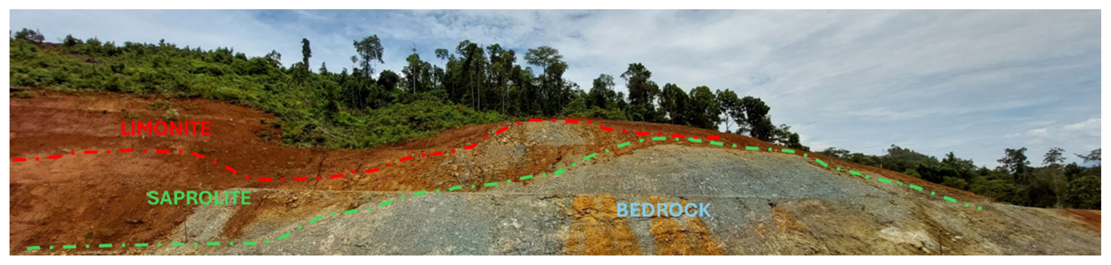
Based on this geological framework, modeling domains are defined vertically as Limonite (LIM), Saprolite (SAP), and Bedrock (BRK) (Figure 2), reflecting the primary mineralogical and geochemical contrasts governing grade variability and spatial continuity.

4.2. Dataset Presentation

The dataset comprises 337 vertical diamond drillholes (DDH) with downhole geochemical assays for Ni, Co, Fe, Si, Mg, Cr, Al, Mn, and Ca, together with lithological logging performed by a geologist. Due to operational and analytical constraints, not all variables are available for every sample, resulting in an incomplete multivariate dataset.
In addition to the drillhole information, Electrical Resistivity Tomography (ERT) data are available. These geophysical measurements provide complementary information on resistivity contrasts, which are associated with contacts between lithological units and variations in weathering intensity.
Three primary lithological codes are defined from geological logging: limonite (LIM), saprolite (SAP), and bedrock (BRK). An additional earthy saprolite domain (ESAP) is delineated based on geochemical criteria, as it is not consistently distinguishable visually in core. This unit reflects intermediate geochemical characteristics between LIM and SAP and therefore may be treated as a separate modeling domain.
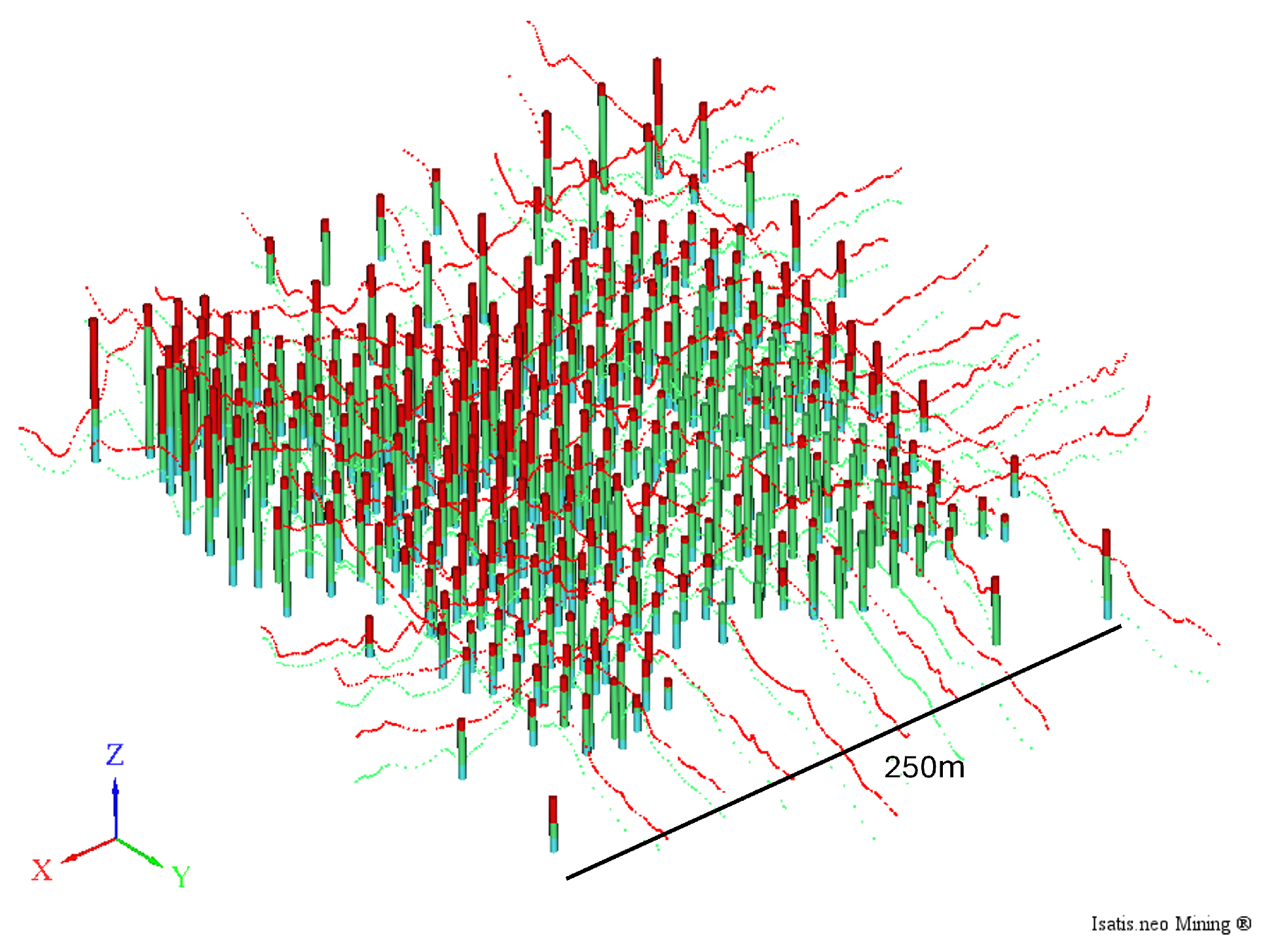
Figure 3 shows a three-dimensional perspective view of the dataset. Cylinders represent drillholes, and points correspond to ERT measurements. Colors indicate lithological domains. Spatial coordinates are omitted for confidentiality reasons. The vertical axis (Z) is vertically exaggerated by a factor of 2.
ERT lines are regularly spaced at approximately 25 × 25 m. The drilling grid exhibits variable spacing: the coarser areas are spaced at approximately 25 × 25 m, while the grade-control drilling follows a tighter pattern of approximately 12.5 × 12.5 m. The average drillhole length is about 15 m, with depths ranging from 5 m to 52 m.
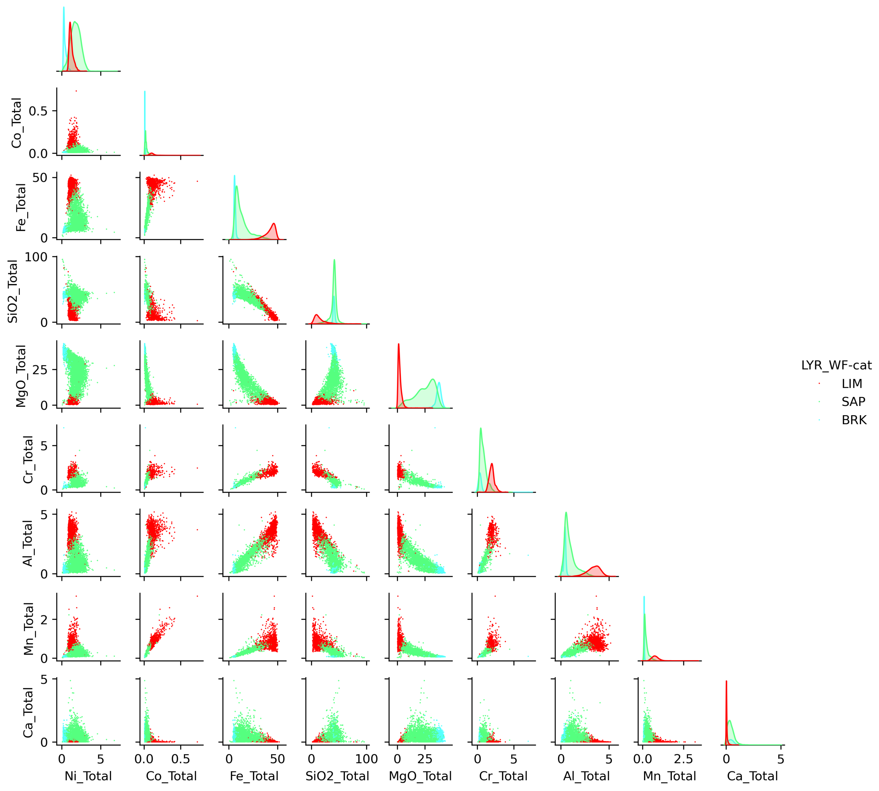
The geochemical variables exhibit complex multivariate relationships as shown in the scatterplot matrix in Figure 4.
The observed correlations are consistent with the supergene processes controlling lateritic nickel formation. A strong negative correlation between Fe and Si, and between Fe and Mg, reflects progressive lateritization, where Mg and Si are leached while Fe is residually enriched in the limonite horizon. Cobalt shows a positive correlation with Fe, consistent with its preferential association with iron oxyhydroxides. Nickel exhibits domain-dependent behavior, being associated with Fe in limonite and with Mg-silicates in saprolite. Aluminum generally follows Fe, reflecting enrichment in clay and iron-rich horizons.

4.3. Results and Discussion

The first step in applying the probabilistic modeling workflow is data preparation. The modeling area is defined by a delimiting polygon with an approximate surface area of 79 m2, and only samples located within this boundary are retained for estimation. A Selective Mining Unit (SMU) grid with dimensions of 12.5 × 12.5 × 2 m is then generated. This grid is subsequently refined to a 5 × 5 × 2 discretization, producing a point-support grid with dimensions of 2.5 × 2.5 × 1 m that is also clipped to the modeling polygon.
Vertically, the simulation grid is bounded at the top by the topographic surface and at the bottom by a surface interpolated from the drillhole end-of-hole depths. This lower surface is extended downward by 10 m to provide a conservative buffer, ensuring that the modeled domain fully encompasses the deepest mineralized intervals and avoids artificial truncation effects near the base of the drill coverage.
From the nine available geochemical variables, six were selected for modeling: Ni, Co, Fe, Si, Mg, and Al. The remaining variables were excluded because they do not materially influence the downstream resource evaluation or metallurgical considerations addressed in this study.
Although lateritic geochemical data may exhibit compositional behavior, the six variables retained here do not define a closed composition, because the unmodeled remainder is non-negligible. The selected subset is therefore not constrained by a constant sum, and ratio transformation was not applied. Additionally, the missing values will be imputed, and standard multivariate imputation algorithms generally do not enforce constant-sum constraints. Instead, the variables were modeled directly and the results were validated through reproduction of marginal distributions, spatial continuity, and multivariate relationships.
The selected variables were composited per domain (LIM, SAP, and BRK) using 1 m intervals. Cell declustering was performed using a 50 m × 50 m window. The resulting weights were used in the calculation of the experimental variograms and the Gaussian anamorphosis.
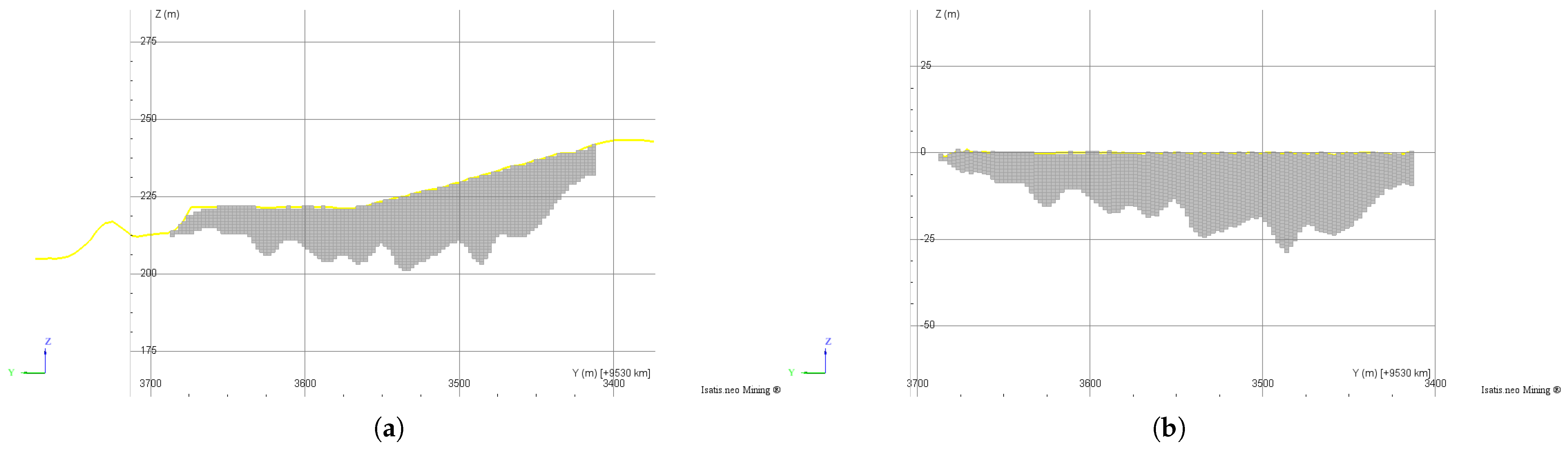
Both the sample data and the point-support grid were unfolded using the topographic surface as the reference, under the assumption that the weathering profile approximately follows the topography. The unfolding was performed in full three dimensions using a tetrahedral model, ensuring that all shifts were applied vertically so that drillholes remain vertical in the unfolded coordinate system.
Figure 5 shows a vertical section of the grid in real-world coordinates and the unfolded grid, together with the topographic surface represented as a yellow wireframe.
Missing data were handled using multivariate imputation per domain. The inputs to the imputation procedure consist of the direct variograms, modeled in Gaussian units, for the six selected geochemical variables, together with the number of Gaussian components used to approximate the multivariate distribution. A total of 100 imputation realizations were generated using six Gaussian components.
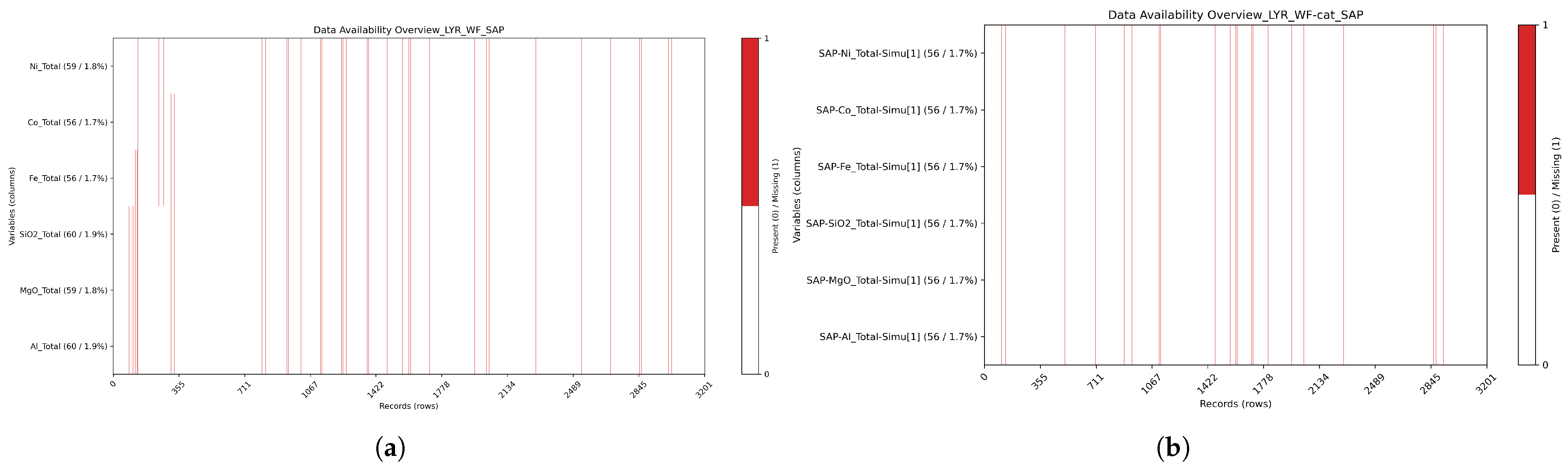
Figure 6 presents a visual summary of data availability for domain SAP before and after imputation. Note that samples for which all variables are missing cannot be imputed. In this area, the majority of samples were already isotopic, and consequently only a small subset required imputation. The output of this step is a set of 100 complete multivariate datasets.
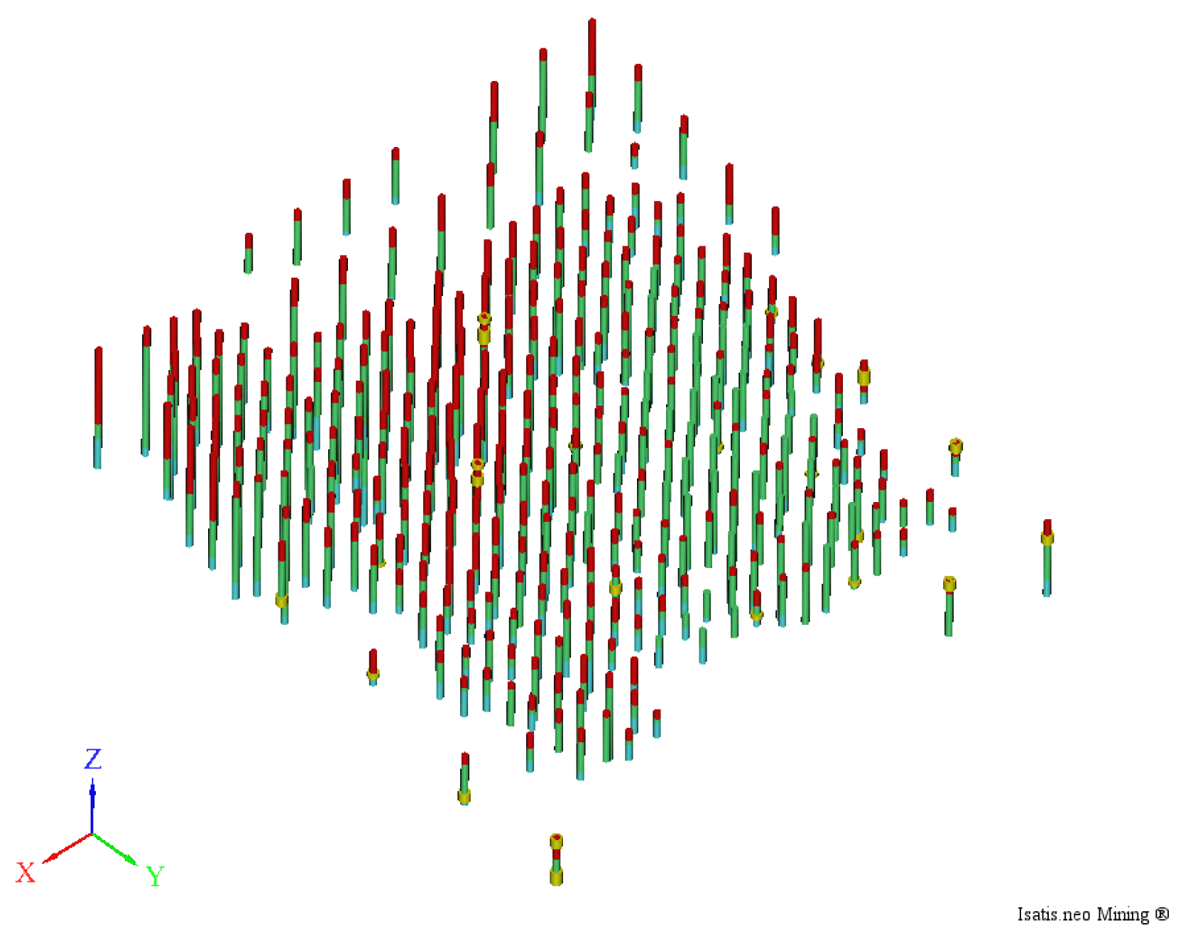
Figure 7 shows the spatial locations of the imputed samples highlighted in yellow.
Each of the 100 complete datasets was transformed using PPMT on a per domain basis. The number of PPMT iterations was set to 85, 50, and 70 for LIM, SAP, and BRK, respectively. The iteration counts were selected to ensure stabilization of the projection index, which measures the deviation from Gaussianity along the projection identified at each iteration.
For the PGS step, local lithological proportions were first estimated from the data in the unfolded grid using an SPDE-based methodology [20]. In this framework, the spatial distribution of category probabilities is modeled as a latent Gaussian random field governed by a stochastic partial differential equation (SPDE). The approach provides smooth spatial estimates of the probability of occurrence of each lithological unit while honoring the categorical observations. These probabilities correspond to the expected values of the indicator variables and are subsequently used to locally adjust the truncation thresholds in the PGS.
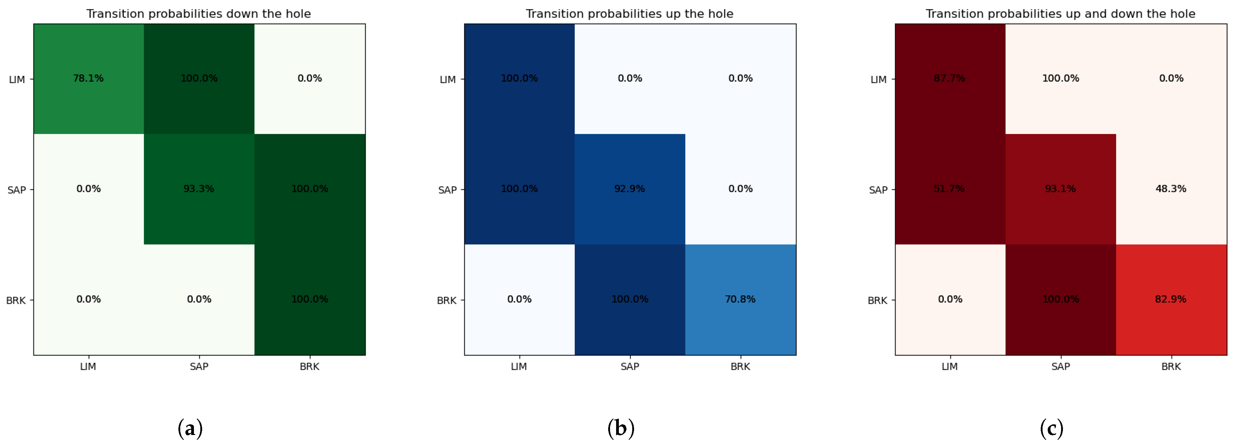
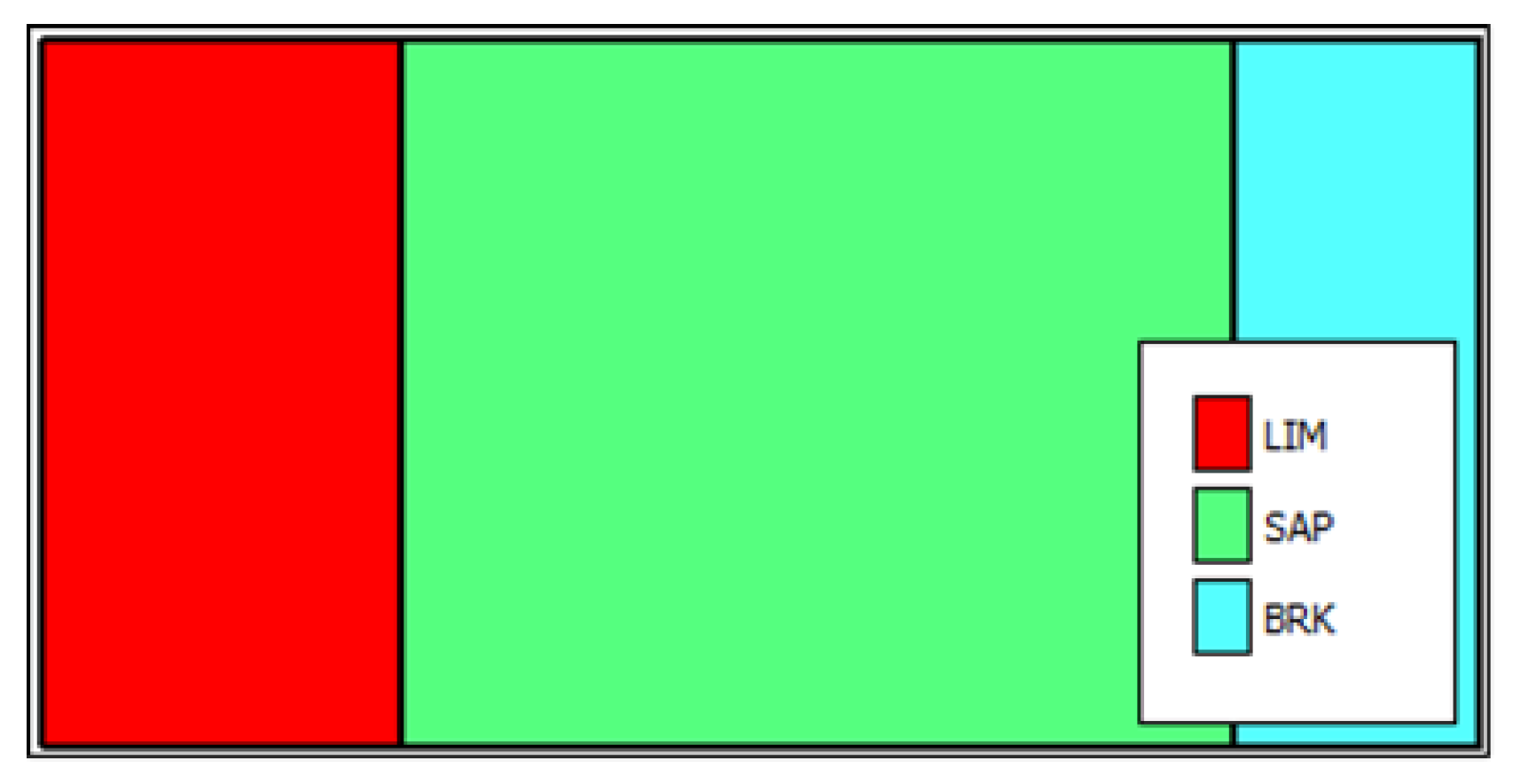
The transition probability matrices (Figure 8) were calculated separately for the downhole and uphole directions and then combined. The diagonal entries represent the proportion of samples that remain in the same lithology. The off-diagonal entries represent, for samples that do not remain in the same lithology, the proportion that transition to each of the other lithologies. These matrices were used to define the truncation rule. The truncation rule adopted in this study is shown in Figure 9.
The variogram model for the underlying Gaussian variable was automatically inferred from the indicator variograms. A total of 100 plurigaussian realizations were then generated in the unfolded grid using a horizontally oriented search neighborhood with radii of 100 × 100 × 10 m, divided into four angular sectors with a maximum of 10 samples per sector. Conditioning was performed using drillhole data only.
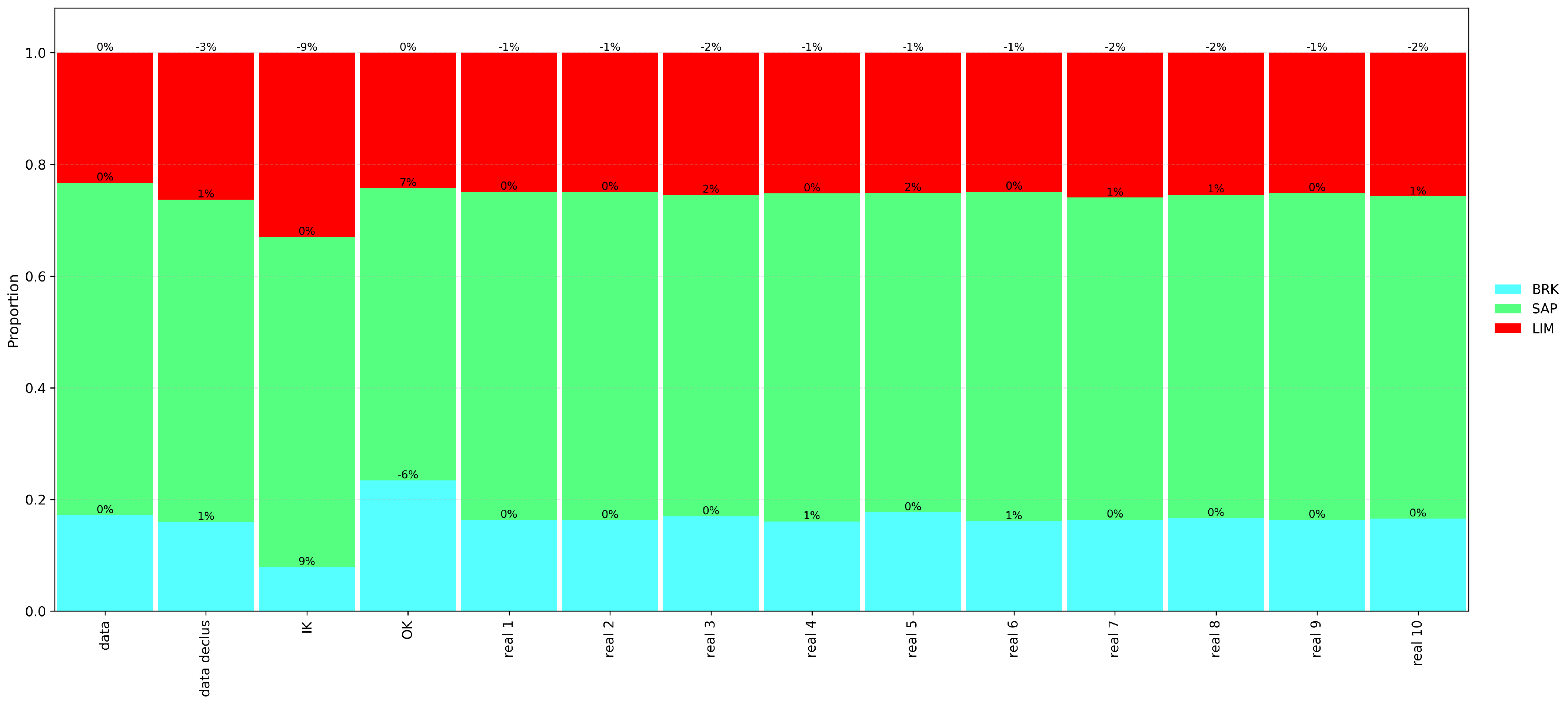
For PGS validation, vertical and horizontal sections were first reviewed and visually interpreted by a geologist. The simulated lithological variables were also compared qualitatively with the ERT data. Finally, the global lithological proportions were evaluated against declustered drillhole data. The comparison includes the raw and declustered data proportions, the proportions derived from the indicator kriging model, the model based on interpreted surfaces, and the proportions obtained from the PGS realizations. For readability, only the first 10 realizations (out of 100) are shown in Figure 10. The difference in proportions relative to the data proportions is indicated above each bar.
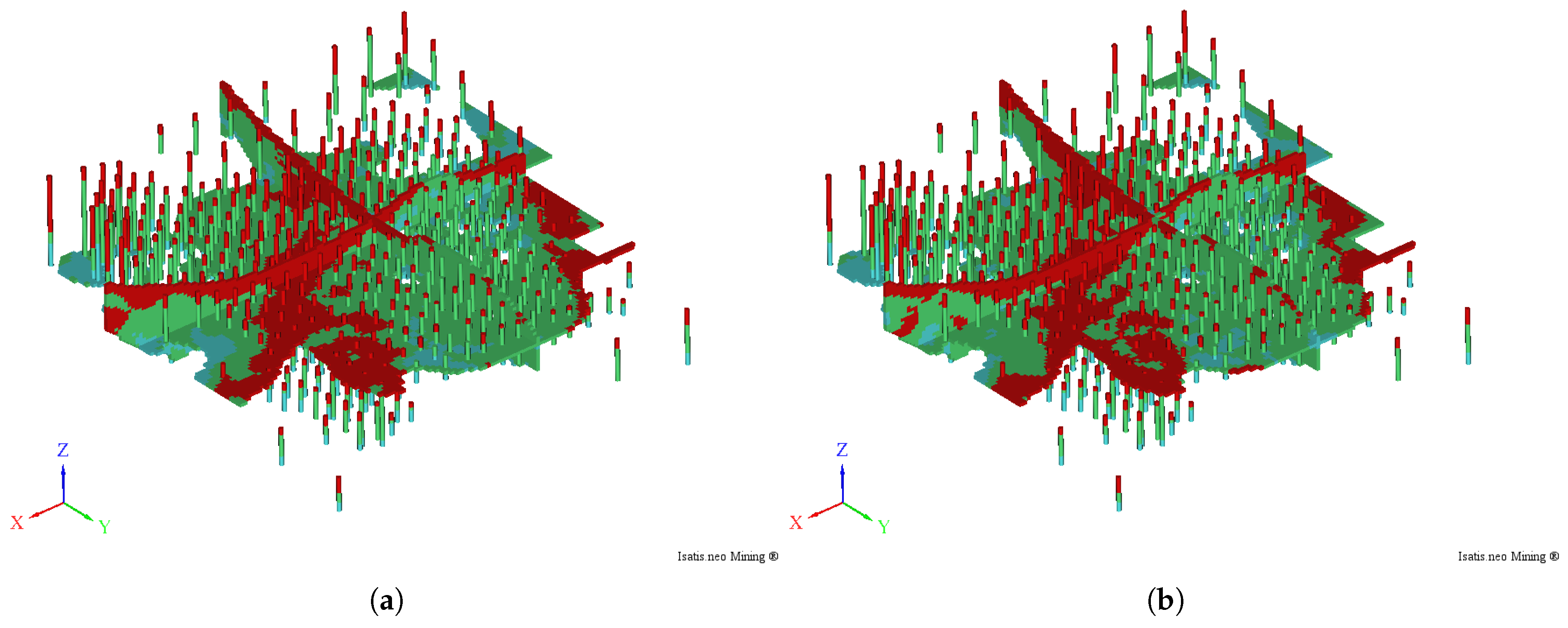
Figure 11 presents a three-dimensional view of the conditioning drillhole data together with cross-sections from two categorical realizations.
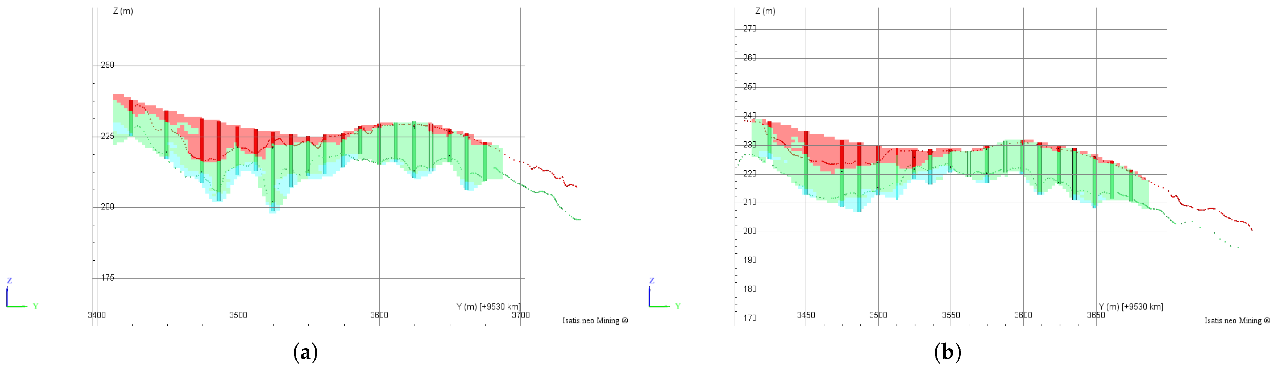
Figure 12 presents two vertical sections extracted from one realization together with the drillholes and ERT data used to assess the consistency of the simulated models.
For the simulation of the PPMT factors, the first step consists of calculating and modeling the variograms. As noted by Barnett et al. [33], it is preferable to model the variograms of the Gaussian-transformed variables rather than the PPMT factors themselves, since each nonlinear transformation applied during PPMT may degrade spatial continuity.
Experimental omni-horizontal and vertical variograms were computed using predefined parameters. The experimental variograms were then automatically fitted with two spherical structures, imposing constraints on the minimum and maximum ranges for each structure in each direction.
For each domain, a total of 100 realizations were generated in the unfolded grid for each PPMT factor using TBS. A horizontally oriented search neighborhood with radii of 75 × 75 × 4 m was adopted, divided into four angular sectors with a maximum of 12 samples per sector. The domain variable in the unfolded grid corresponds to the associated PGS categorical realization as exemplified in Figure 1.
Simulations were conditioned using simple kriging, which implies the assumption of strong stationarity within each domain. When this assumption is not valid, the spatial trend should be explicitly modeled and incorporated into the simulation framework [42].
In this approach, categorical and continuous variables are simulated independently. However, it is also possible to jointly simulate grades and rock types using a PGS co-simulation framework, as proposed by Emery and Silva [43]. In this formulation, the continuous variable is modeled as a transform of a Gaussian random field, while the categorical variable is obtained by truncating one or more Gaussian random fields, with all underlying fields being spatially cross-correlated. This joint modeling allows reproducing the dependencies between grades and lithological units, as well as accounting for the spatial correlation of grades across rock-type boundaries, particularly in the presence of soft contacts.
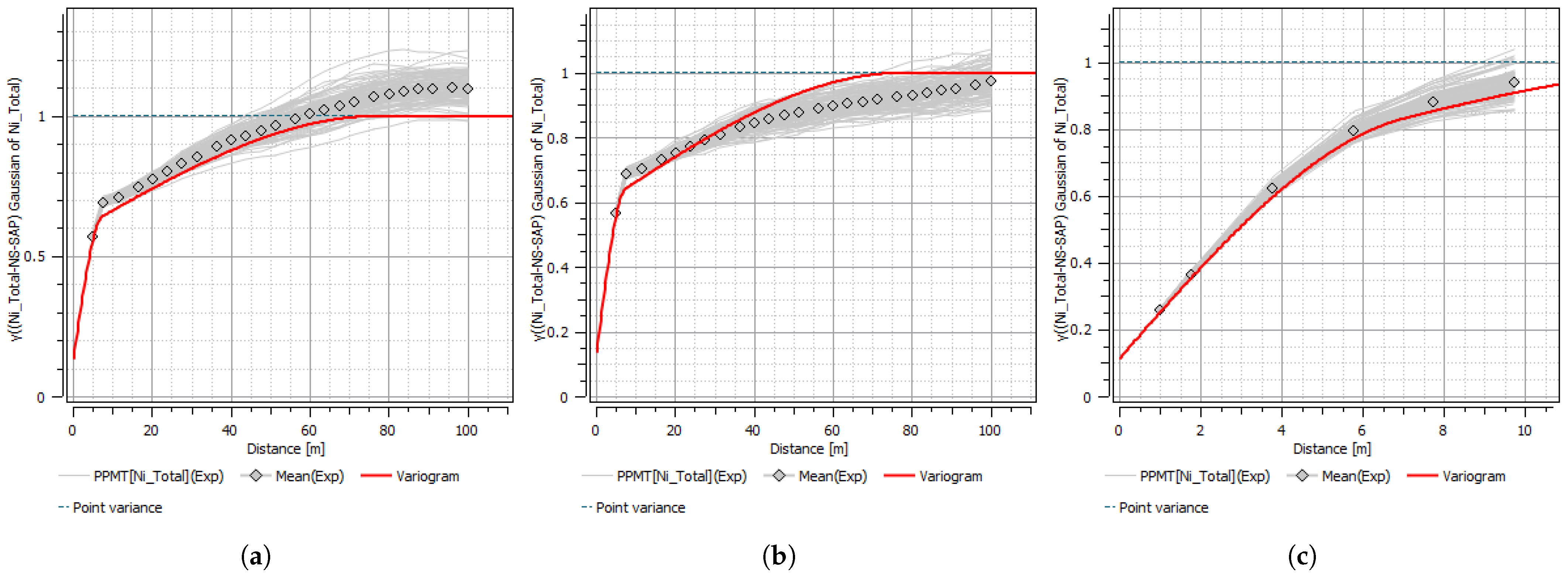
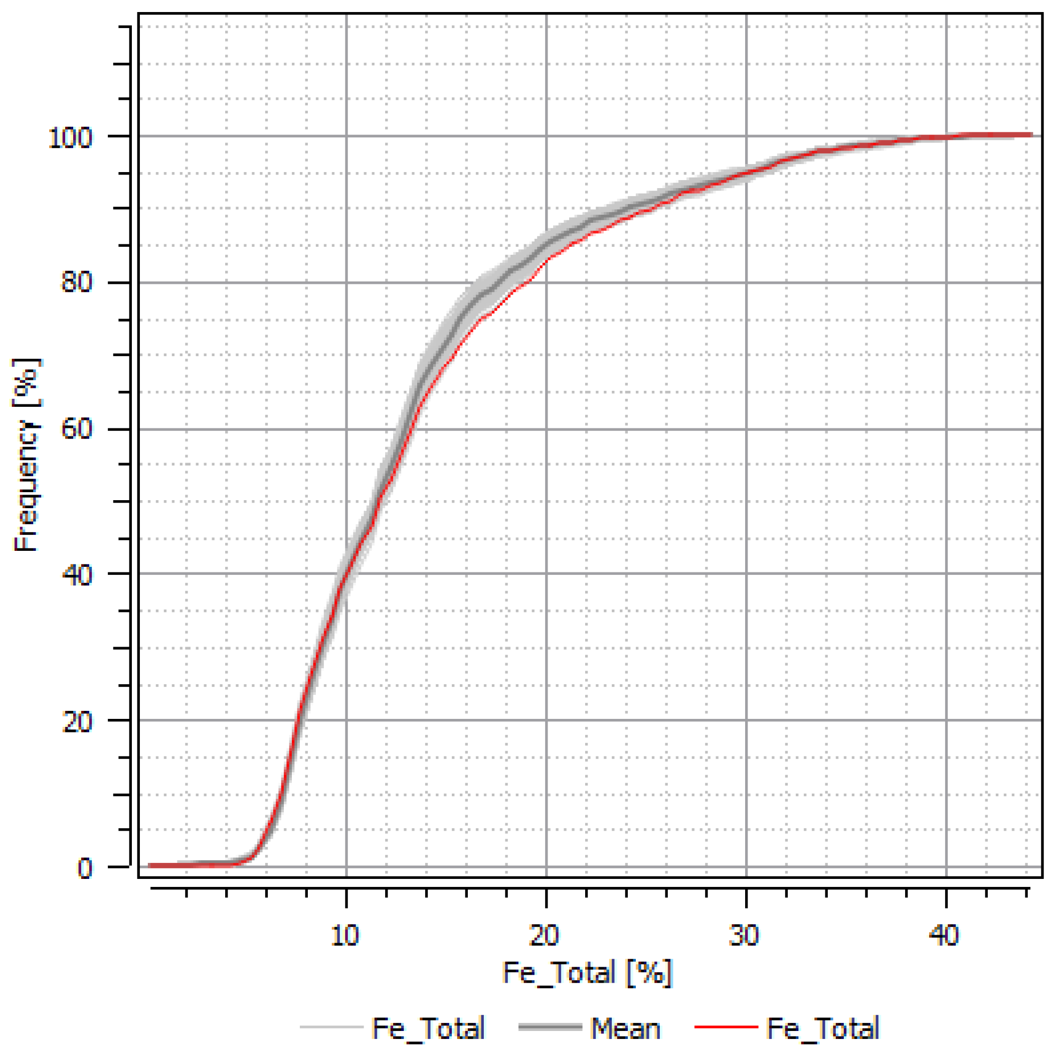
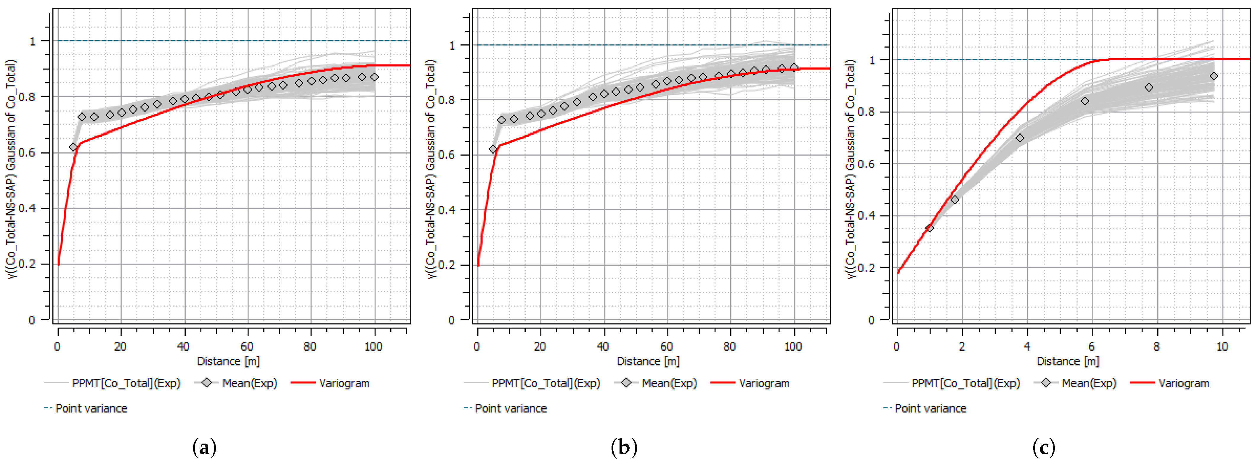
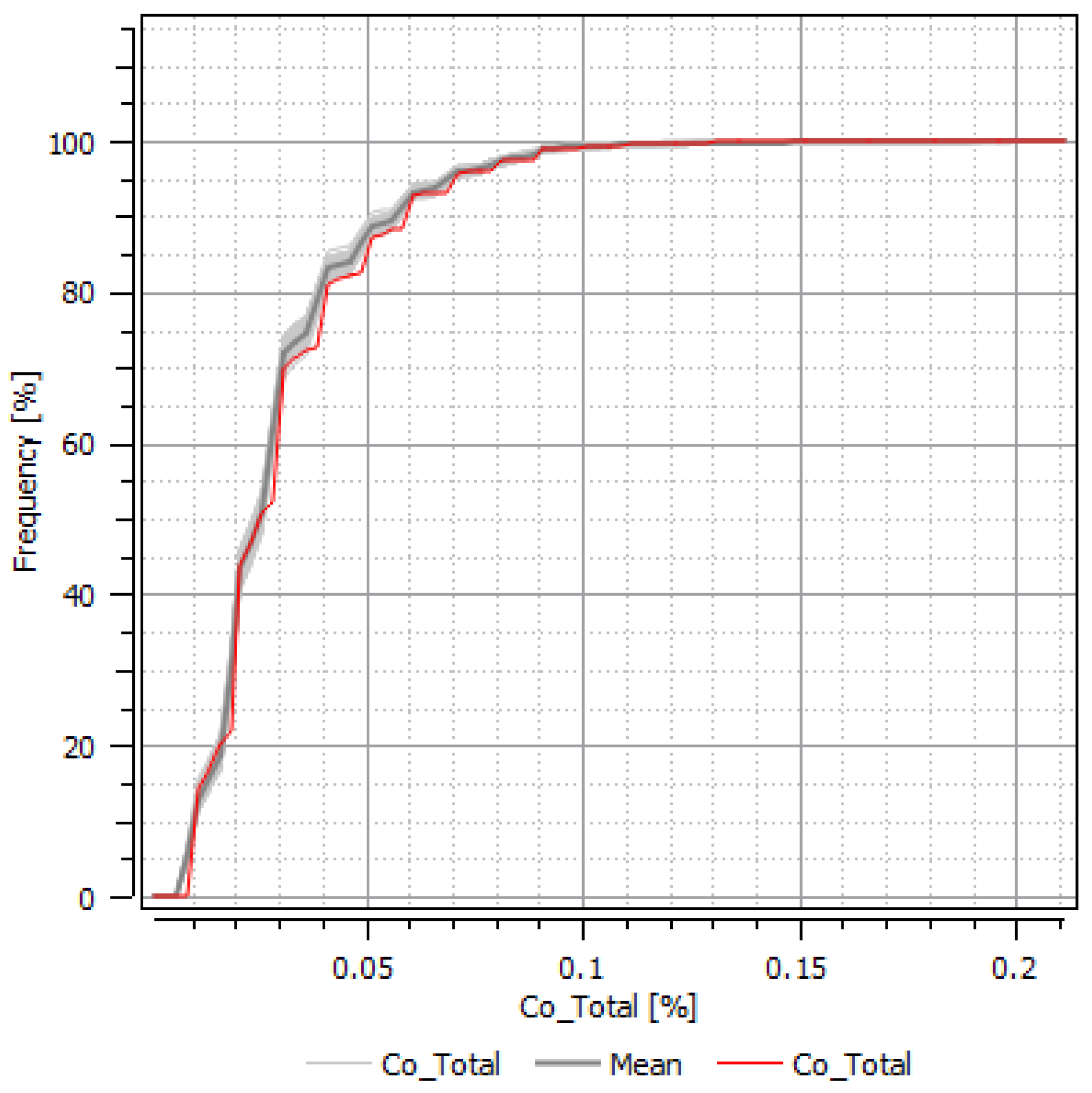
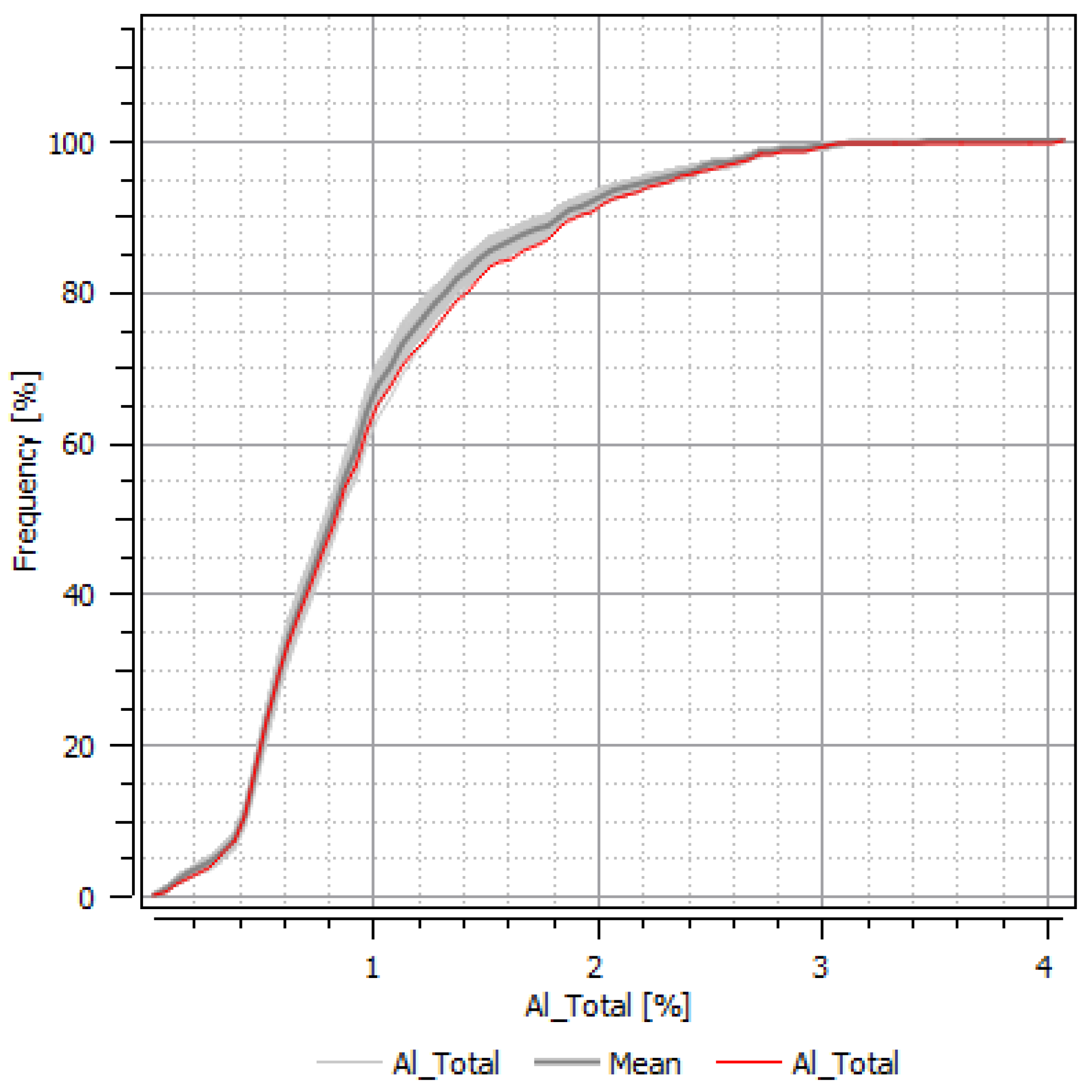
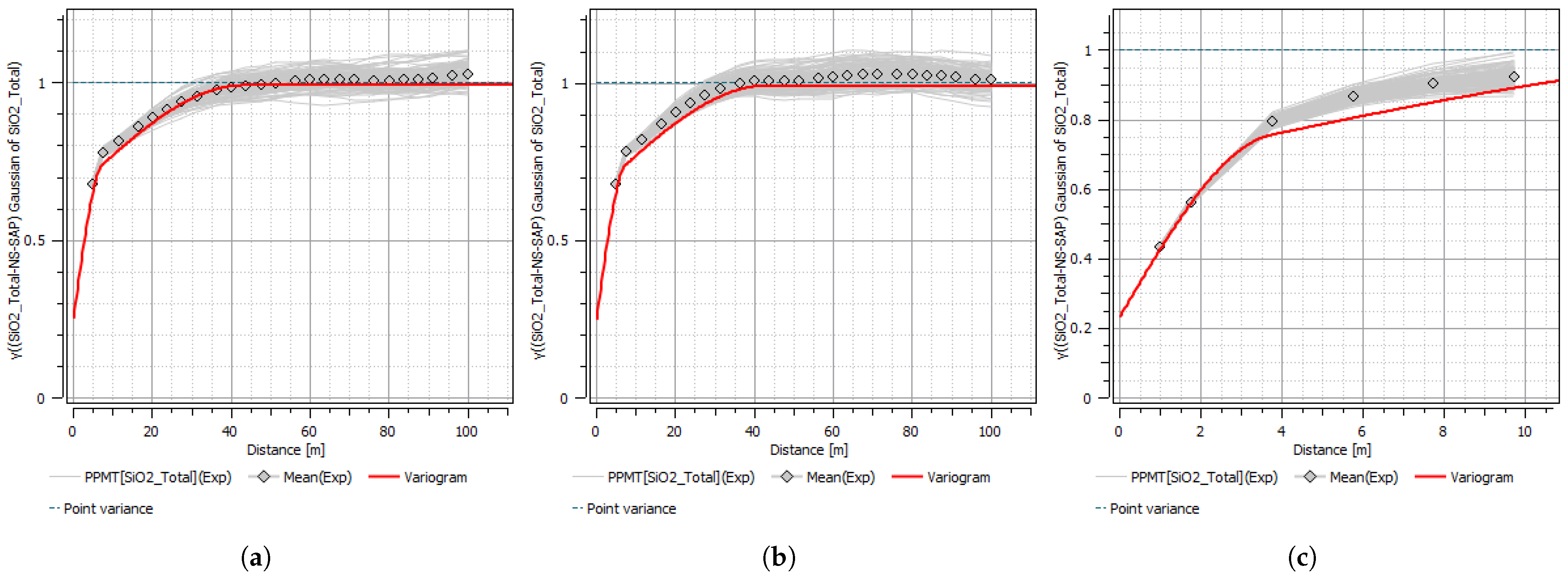
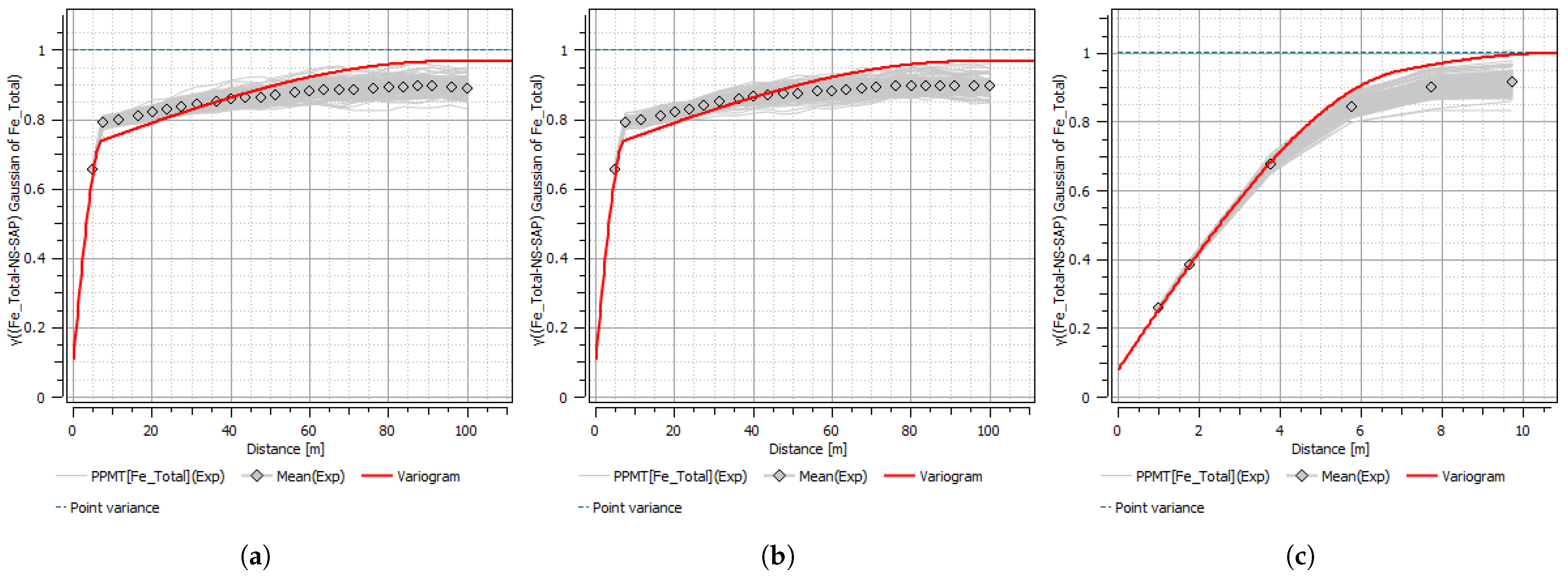
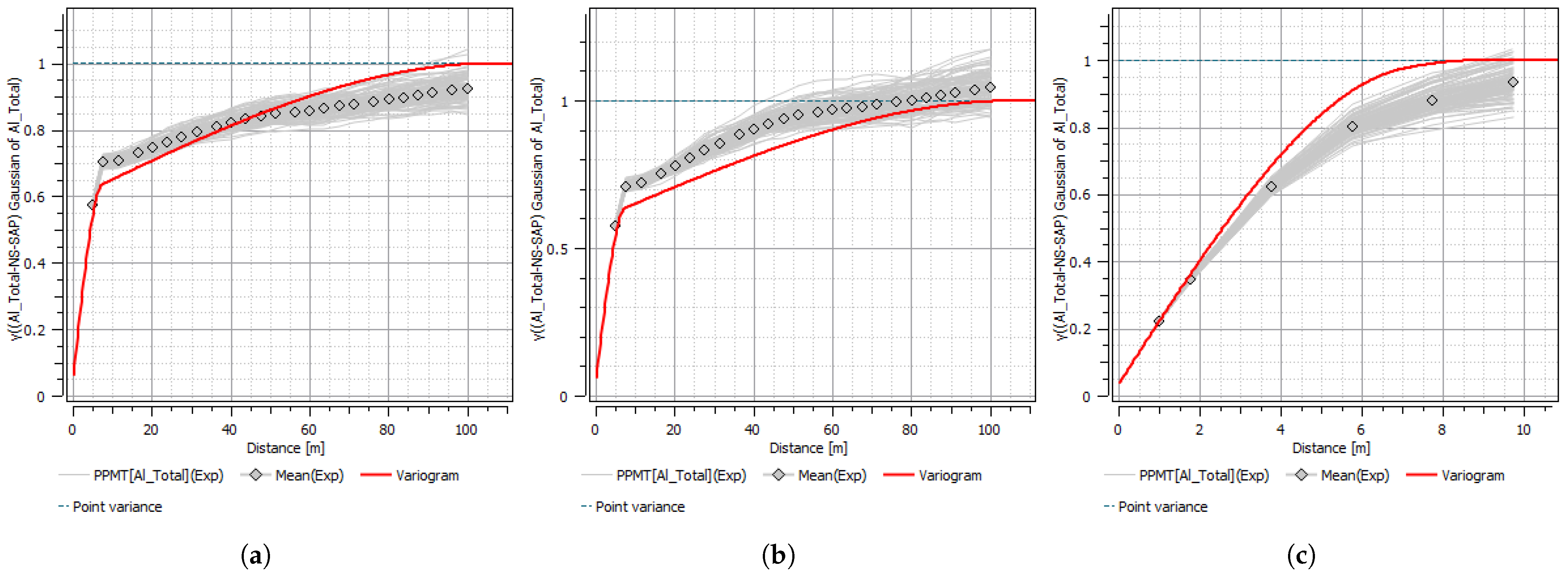
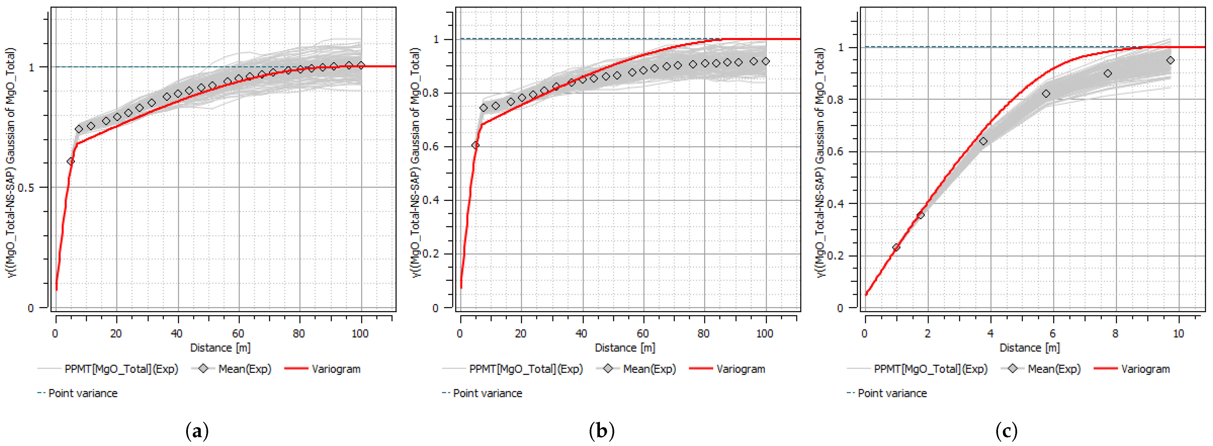
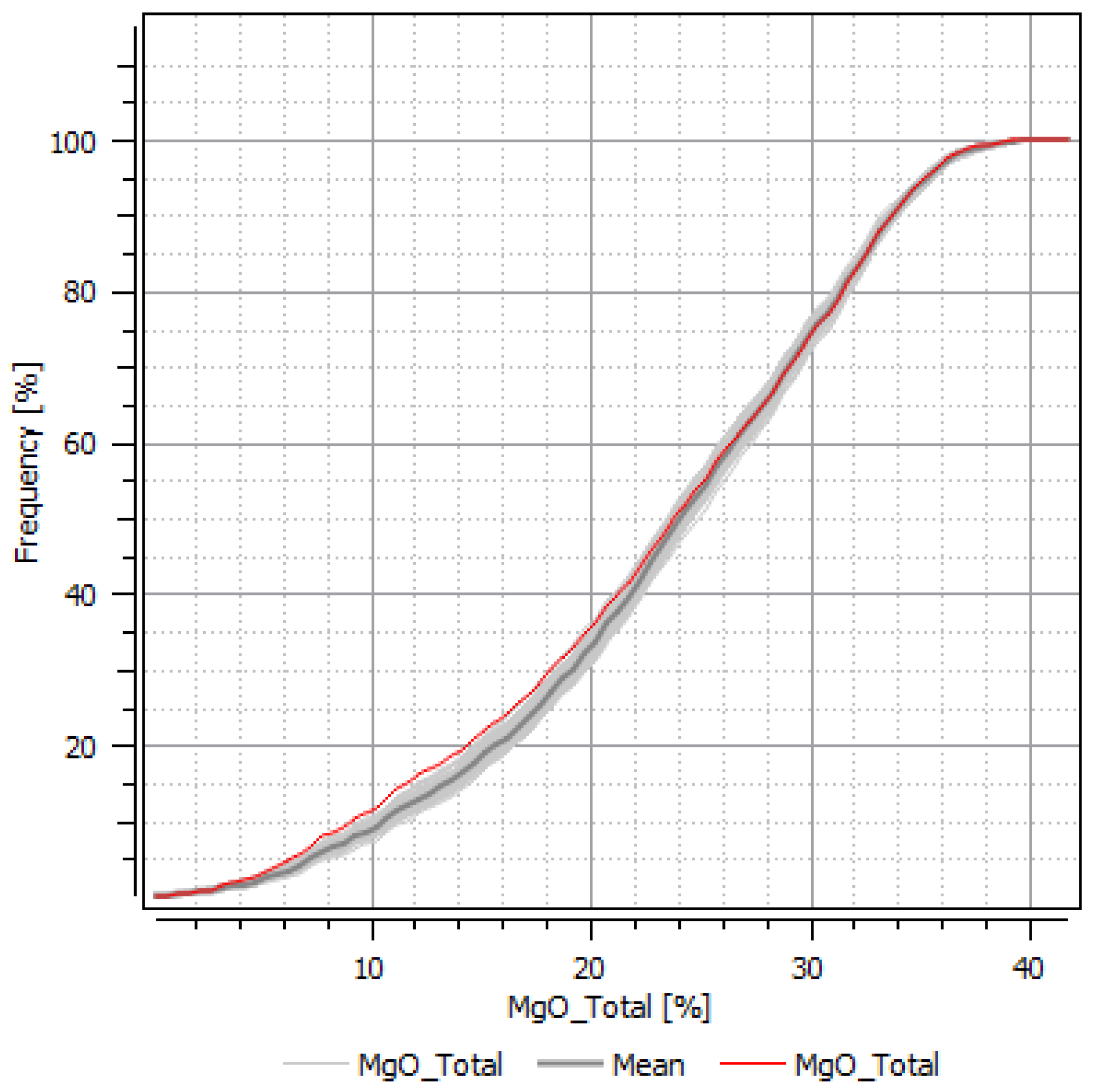
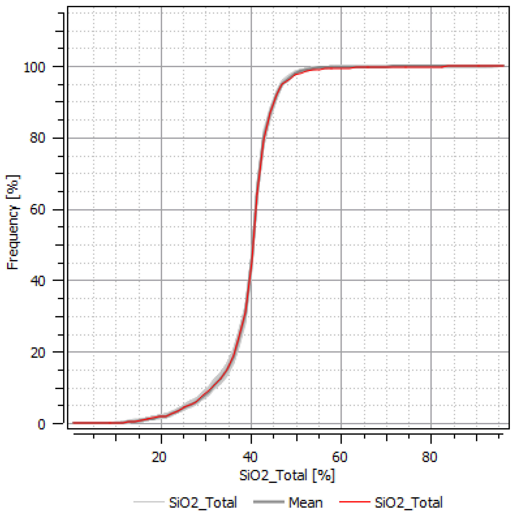
For validation of the continuous variable simulations, the experimental variograms of the simulated PPMT factors (prior to back-transformation) were compared with the Gaussian variogram models used for simulation. After back-transformation, the histograms of the simulated variables were compared with the histograms of the declustered data. Although all domains were simulated, only the results for SAP are presented.
Figure 13 presents the variogram validation results for Ni.
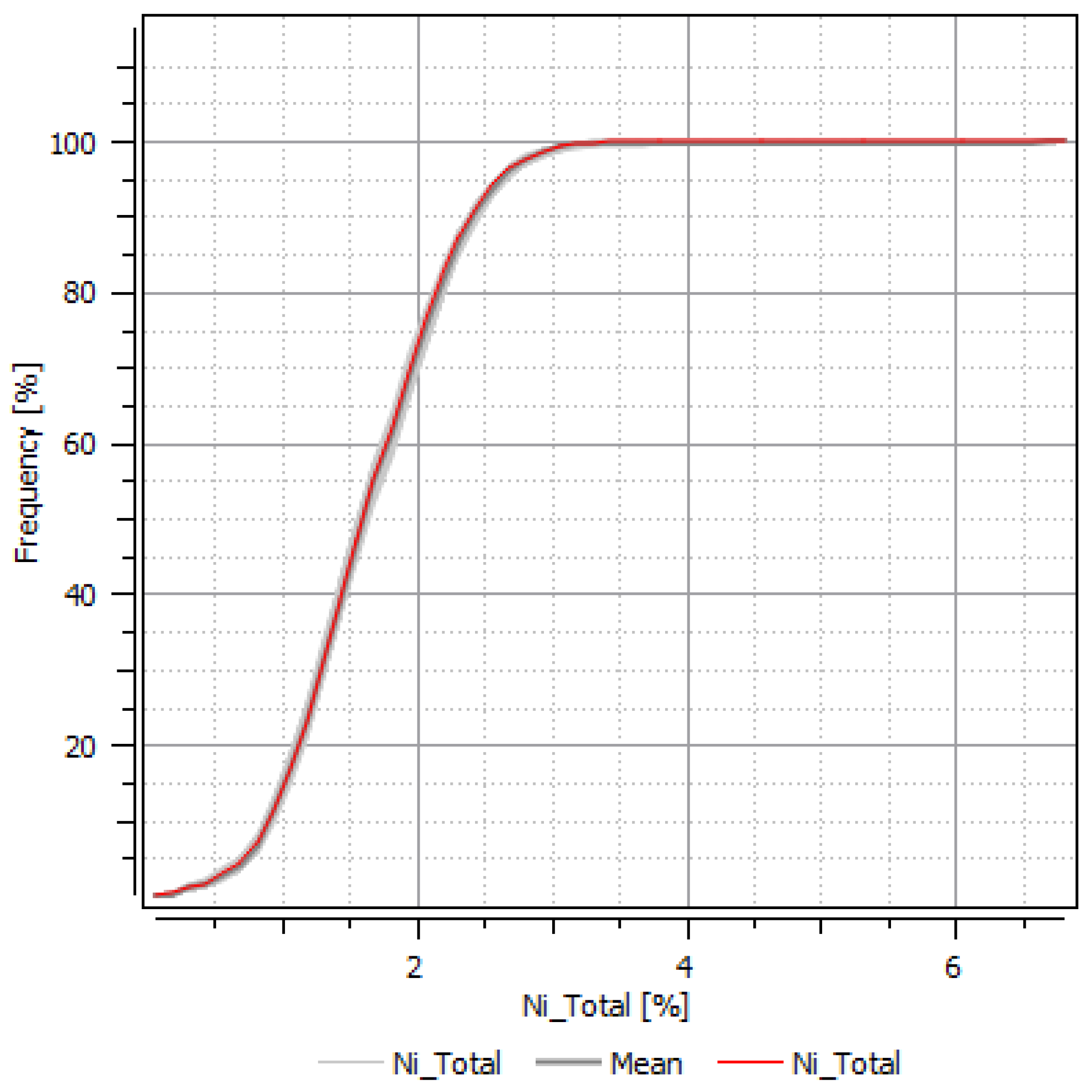
Figure 14 presents the histogram validation results for Ni.
Figure 15 presents the variogram validation results for Fe.
Figure 16 presents the histogram validation results for Fe.
Figure 17 presents the variogram validation results for Co.
Figure 18 presents the histogram validation results for Co.
Figure 19 presents the variogram validation results for Al.
Figure 20 presents the histogram validation results for Al.
Figure 21 presents the variogram validation results for Mg.
Figure 22 presents the histogram validation results for Mg.
Figure 23 presents the variogram validation results for Si.
Figure 24 presents the histogram validation results for Si.
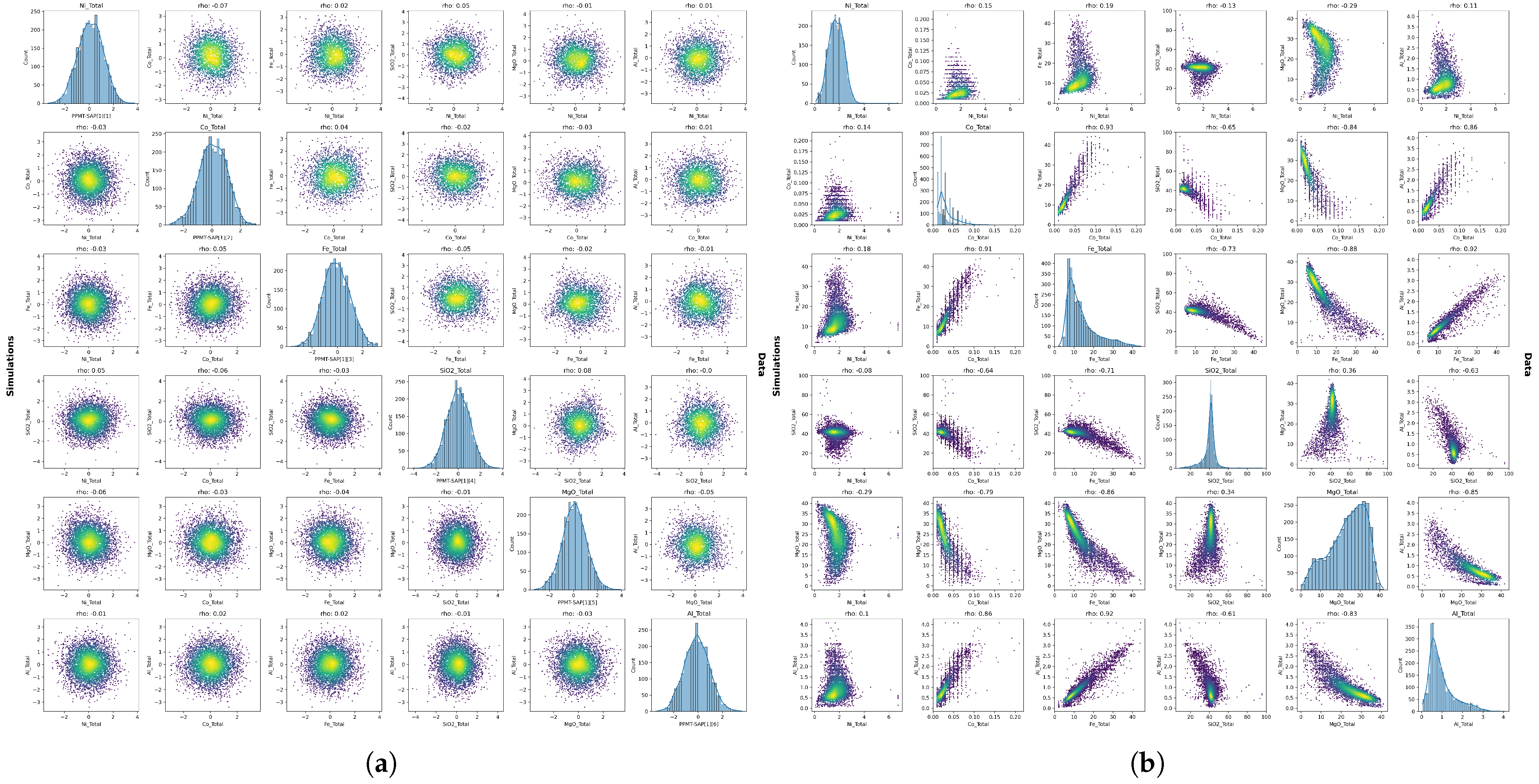
Reproduction of the multivariate relationships was also evaluated. In Figure 25a, the upper triangular matrix presents scatterplots of the PPMT factors computed from the drillhole data (DDH), while the lower triangular matrix shows the corresponding scatterplots of the simulated PPMT factors prior to back-transformation. Figure 25b follows the same structure, displaying the scatterplots after back-transformation.
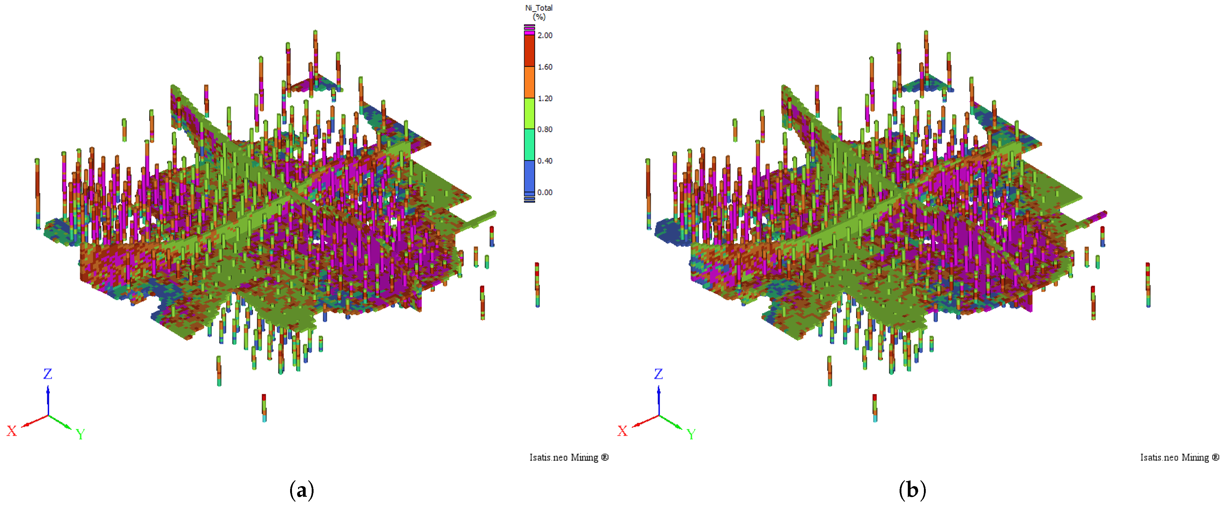
Figure 26 presents a three-dimensional view of the conditioning drillhole data together with cross-sections from two Ni realizations.
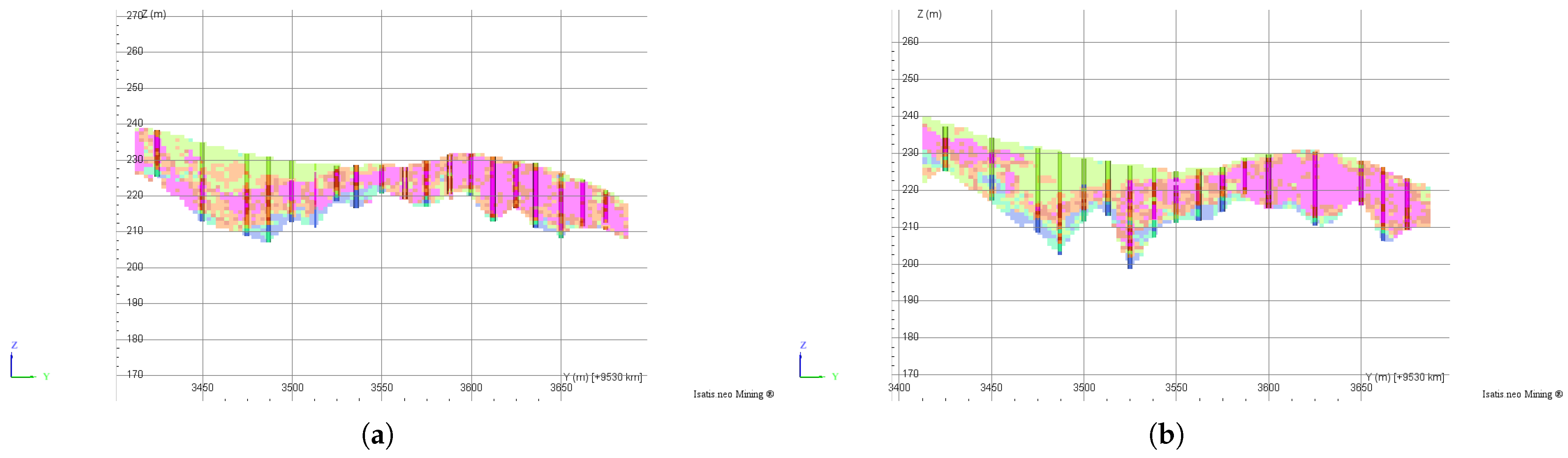
Figure 27 presents two vertical sections extracted from one realization together with the drillholes.
For tonnage calculations, density was assumed constant within each domain. Although density typically exhibits significant vertical variability in lateritic nickel deposits, the density sampling program for the present deposit is still under development.
If density data were available, density should also be simulated. It may be simulated independently, without directly modeling the accumulation (grade × density), as the direct approach has been shown to better reproduce the histogram of the data [44]. However, during upscaling to the SMU support, accumulation should be computed and averaged, and the upscaled grade subsequently obtained by dividing the upscaled accumulation by the upscaled density.
The unfolded realizations were first back-transformed to the original coordinate system. The PGS realizations were then upscaled from the point-support grid to the SMU support, preserving the lithological proportions within each SMU for every realization. Subsequently, the continuous variables were upscaled by averaging the point-support values contained within each SMU.
For each realization, the SMU tonnage per lithology is calculated as the product of the lithological proportion, the SMU volume, and the corresponding density, considering only material above the specified cut-off grade. The SMU average grade per lithology is computed as the weighted average of grades, using the lithological proportions as weights. These calculations are performed for different cut-off grades.
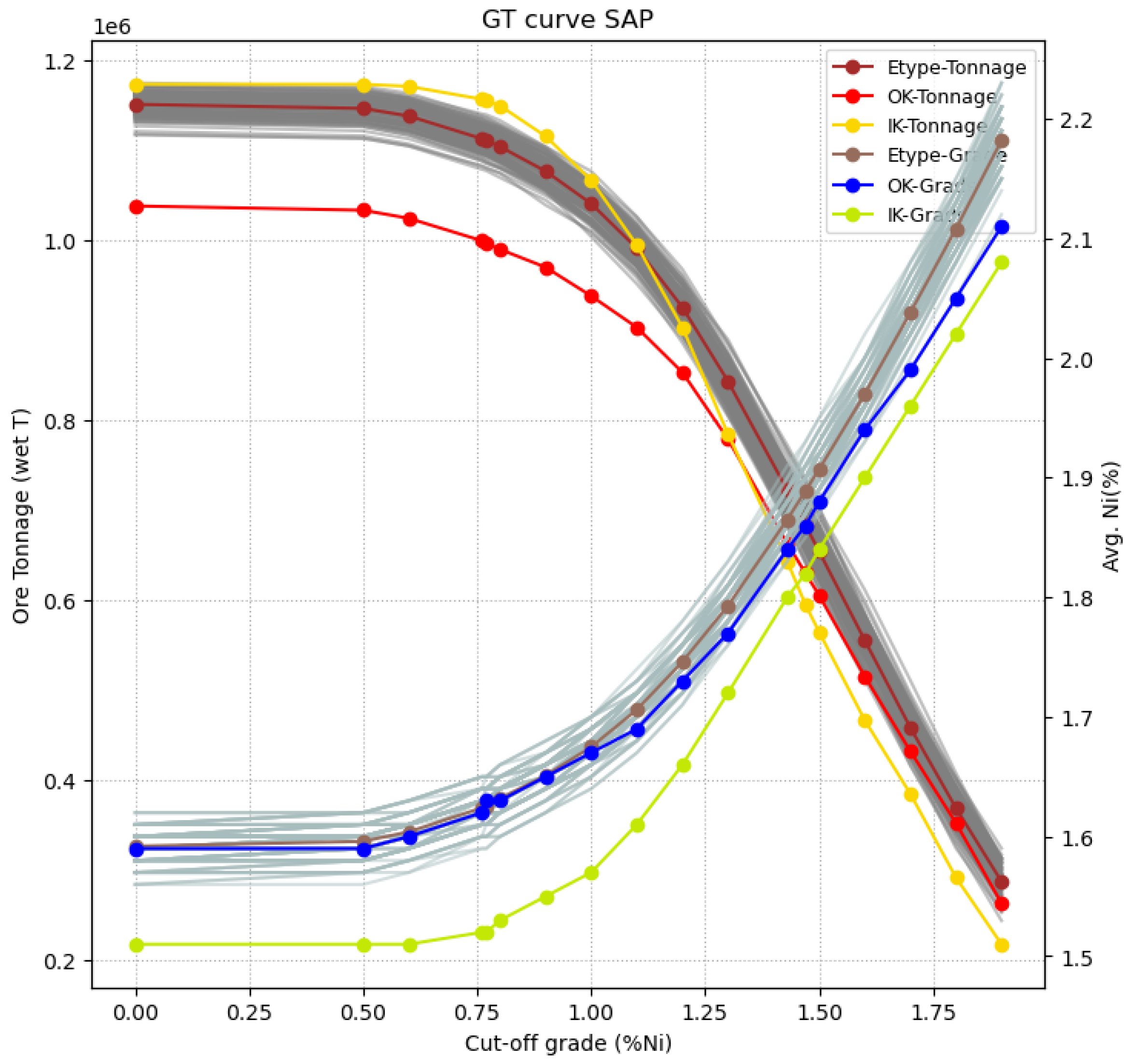
Figure 28 presents the grade–tonnage curves for domain SAP derived from the simulations, compared with (i) a model constructed using ordinary kriging with domains defined deterministically by contact surfaces and (ii) ordinary kriging incorporating proportions estimated from indicator kriging.
The results indicate that PGS successfully reproduces the global declustered lithological proportions and produces realizations consistent with the ERT data. The multivariate imputation step ensures a complete dataset suitable for application of the PPMT transformation. The PPMT transform enables the simulation to reproduce the complex multivariate relationships characteristic of lateritic nickel deposits (Figure 25) while also honoring the declustered distributions and variograms of the individual variables.
The unfolding step contributes to more geologically realistic results for both categorical and continuous variable simulations. After back-transformation to the original coordinate system, the simulated trends follow the weathering profile rather than being artificially aligned along horizontal planes.
The probabilistic workflow enables risk assessment in recoverable resource estimation. Instead of producing a single deterministic grade–tonnage curve, as obtained from kriging-based estimation, the methodology generates an uncertainty bandwidth, allowing evaluation of worst-case, best-case, and expected scenarios. Differences are observed between the simulated tonnages and those derived from ordinary kriging with domains defined deterministically by surfaces. This highlights the limitations of deterministic domain definition in highly variable lateritic environments.
From a short-term perspective, the results can support the assessment of uncertainty related to digline selection. More broadly, the simulated outcomes may be directly applied to resource classification [45] and drillhole spacing analysis [46].

5. Conclusions

This study discusses and integrates the key components required for probabilistic modeling of lateritic nickel deposits and addresses the main challenges associated with these systems, including complex stratigraphic geometry, heterotopic sampling, nonlinear multivariate relationships, and inherent uncertainty.
Application to an Indonesian lateritic nickel deposit shows that the workflow successfully reproduces lithological proportions, spatial continuity, marginal distributions, and multivariate relationships. The unfolding procedure enhances geological realism by aligning simulations with the weathering profile, while PPMT enables high-dimensional simulation without requiring explicit modeling of the full linear model of coregionalization.
The resulting grade–tonnage curves highlight differences compared with deterministic ordinary kriging approaches, particularly when domains are defined by fixed surfaces. Rather than producing a single resource estimate, the approach generates an ensemble of equiprobable scenarios, allowing explicit quantification of uncertainty and evaluation of downside and upside risk.
Beyond recoverable resource estimation, the workflow provides a foundation for downstream applications such as mineral resource classification, short-term mine planning, and drillhole spacing optimization.

Author Contributions

R.R. conceptualization, methodology, software, visualization, validation, writing; J.A. conceptualization, data curation, methodology, software, visualization, validation, writing; S.Y. supervision, project administration. All authors have read and agreed to the published version of the manuscript.

Funding

This research received no external funding.

Data Availability Statement

The data used in this study are the property of Vale Indonesia and cannot be shared publicly.

Acknowledgments

The authors sincerely thank the three anonymous reviewers for their careful evaluation and valuable insights, which significantly improved the clarity and quality of this manuscript. The authors are also grateful to Vale Indonesia for kindly granting permission to publish the results of this study. All results presented in this work were generated using Isatis.neo and Python scripting.

Conflicts of Interest

Author Roberto Rolo was employed by the company Geovariances. Authors Jafar Arief and Selvi Yuminti were employed by the company Vale Indonesia. All authors declare that the research was conducted in the absence of any commercial or financial relationships that could be construed as a potential conflict of interest.

References

  1. Deutsch, C.V. The Place of Geostatistical Simulation through the Life Cycle of a Mineral Deposit. Minerals 2023, 13, 1400. [Google Scholar] [CrossRef]
  2. Conoras, W.A.K.; Lamburu, A.A. Modeling and Resource Classification Lateritic Nickel Deposits on a Heterogeneous Block in The Haul-Sagu Area using Estimation and Simulation Geostatistical Method. J. Phys. Conf. Ser. 2020, 1569, 042079. [Google Scholar] [CrossRef]
  3. Richmond, A. Conditional Simulation of a Nickel Laterite Deposit using Unfolding. In Proceedings of the 36th International Symposium on the Application of Computers and Operations Research in the Mineral Industry (APCOM 2013), Porto Alegre, Brazil, 4–8 November 2013; p. 6. [Google Scholar]
  4. Toro, J.A.A.d.; Carballo-Pena, A.; Estevez-Cruz, E.; Cobas-Botey, R.M. Modelaje probabilístico y cuantificación de la incertidumbre de los horizontes de la corteza de meteorización del depósito de níquel San Felipe. Minería Geol. 2024, 40, 1–24. [Google Scholar]
  5. Dagasan, Y.; Erten, O.; Renard, P. Multiple-point statistical simulation of the ore boundaries for a lateritic bauxite deposit. Stoch. Environ. Res. Risk Assess. 2019, 33, 865–878. [Google Scholar] [CrossRef]
  6. Deraisme, J.; Bertoli, O.; Epinoux, P. Multivariate block simulations of a lateritic nickel deposit and post-processing of a representative subset. J. S. Afr. Inst. Min. Metall. 2014, 114, 673–680. [Google Scholar]
  7. de Freitas Silva, M.; Dimitrakopoulos, R. Simulation of weathered profiles coupled with multivariate block-support simulation of the Puma nickel laterite deposit, Brazil. Eng. Geol. 2016, 215, 108–121. [Google Scholar] [CrossRef]
  8. Neves, C.; Costa, J.; Souza, L.; Guimaraes, F.; Dias, G. Methodology for Defining the Optimal Drilling Grid in a Laterite Nickel Deposit Based on a Conditional Simulation; Springer: Berlin/Heidelberg, Germany, 2023; pp. 151–162. [Google Scholar] [CrossRef]
  9. Isatelle, F.; Rivoirard, J. Mineral Resources classification of a nickel laterite deposit: Comparison between conditional simulations and specific areas. J. S. Afr. Inst. Min. Metall. 2019, 119, 871–882. [Google Scholar] [CrossRef]
  10. Renaldy; Heriawan, M.N.; Morales, A.T. A Comparative Study of Conditional Simulation and Specific Area Methods for Nickel Laterite Mineral Resource Classification: Insights from Central Halmahera, North Maluku, Indonesia. Min. Metall. Explor. 2026, 43, 497–509. [Google Scholar] [CrossRef]
  11. Deutsch, C.V. Practical Unfolding for Geostatistical Modelling of Vein-Type and Complex Tabular Mineral Deposits. In Proceedings of the 32nd International Symposium on the Application of Computers and Operations Research in the Mineral Industry (APCOM 2005), Tucson, AZ, USA, 30 March–1 April 2005; pp. 197–202. [Google Scholar]
  12. Latifi, A.M.; Boisvert, J.B. Stratigraphic Coordinate Transformation. In Geostatistics Lessons; Deutsch, J.L., Ed.; 2022; Available online: https://geostatisticslessons.com/lessons/stratcoords (accessed on 25 February 2026).
  13. Isatis.neo User Guide. Datamine Software. 2026. Available online: https://docs.dataminesoftware.com/IsatisNeo/Latest/Isatis-Users-Guide/garde-User-Guide.html (accessed on 25 February 2026).
  14. Boisvert, J.B.; Manchuk, J.G.; Deutsch, C.V. Kriging in the Presence of Locally Varying Anisotropy Using Non-Euclidean Distances. Math. Geosci. 2009, 41, 585–601. [Google Scholar] [CrossRef]
  15. Alabert, F. Stochastic Imaging of Spatial Distributions Using Hard and Soft Information. Master’s Thesis, Stanford University, Stanford, CA, Canada, 1987. [Google Scholar]
  16. Armstrong, M.; Galli, A.; Beucher, H.; Loc’h, G.; Renard, D.; Doligez, B.; Eschard, R.; Geffroy, F. Plurigaussian Simulations in Geosciences; Springer: Berlin/Heidelberg, Germany, 2011. [Google Scholar]
  17. Silva, D. Enhanced Geologic Modeling of Multiple Categorical Variables. Ph.D. Thesis, University of Alberta, Edmonton, AB, Canada, 2018. [Google Scholar]
  18. Strebelle, S.B. Sequential Simulation Drawing Structures from Training Images; Stanford University: Stanford, CA, USA, 2000. [Google Scholar]
  19. Mariethoz, G.; Renard, P.; Straubhaar, J. The direct sampling method to perform multiple-point geostatistical simulations. Water Resour. Res. 2010, 46, W11536. [Google Scholar] [CrossRef]
  20. Desassis, N.; Renard, D.; Beucher, H.; Petiteau, S.; Freulon, X. A Pairwise Likelihood Approach for the Empirical Estimation of the Underlying Variograms in the Plurigaussian Models. arXiv 2015, arXiv:1510.02668. [Google Scholar]
  21. Erten, G.E.; da Silva, C.Z.; Boisvert, J. Decorrelation and Imputation Methods for Multivariate Modeling. In Applied Spatiotemporal Data Analytics and Machine Learning; Chapter 1; Maucec, D.M., Yarus, P.J.M., Coburn, D.T.C., Pyrcz, P.M.J., Eds.; IntechOpen: London, UK, 2024. [Google Scholar] [CrossRef]
  22. Barnett, R.M.; Deutsch, C.V. Multivariate imputation of unequally sampled geological variables. Math. Geosci. 2015, 47, 791–817. [Google Scholar] [CrossRef]
  23. Silva, D.S.; Deutsch, C.V. Multivariate data imputation using Gaussian mixture models. Spat. Stat. 2018, 27, 74–90. [Google Scholar] [CrossRef]
  24. Aitchison, J. The statistical analysis of compositional data. J. R. Stat. Soc. Ser. B (Methodol.) 1982, 44, 139–160. [Google Scholar] [CrossRef]
  25. Barnett, R.M.; Deutsch, C.V. Why the Log in Logratios? Technical Report CCG Paper 2013-108; Centre for Computational Geostatistics (CCG): Edmonton, AB, Canada, 2013. [Google Scholar]
  26. Bassani, M.A.A.; Coimbra Leite Costa, J.F.; Deutsch, C.V. Multivariate geostatistical simulation with sum and fraction constraints. Appl. Earth Sci. 2018, 127, 83–93. [Google Scholar] [CrossRef]
  27. Hotelling, H. Analysis of a Complex of Statistical Variables into Principal Components. J. Educ. Psychol. 1933, 24, 417–441. [Google Scholar] [CrossRef]
  28. Switzer, P.; Green, A.A. Min/Max Autocorrelation Factors for Multivariate Spatial Imaging; Technical report; Stanford University: Stanford, CA, USA, 1984. [Google Scholar]
  29. Barnett, R.M. Projection Pursuit Multivariate Transform. 2017. Available online: https://geostatisticslessons.com/lessons/ppmt (accessed on 26 February 2026).
  30. Leuangthong, O.; Deutsch, C.V. Stepwise Conditional Transformation for Simulation of Multiple Variables. Math. Geol. 2003, 35, 155–173. [Google Scholar] [CrossRef]
  31. Cook, A.; Rondon, O.; Graindorge, J.; Booth, G. Iterative Gaussianisation for Multivariate Transformation. In Proceedings of the Geostatistics Toronto 2021; Avalos Sotomayor, S.A., Ortiz, J.M., Srivastava, R.M., Eds.; Springer International Publishing: Cham, Switzerland, 2023; pp. 21–35. [Google Scholar]
  32. Avalos, S.; Ortiz, J.M. Spatial Multivariate Morphing Transformation. Math. Geosci. 2023, 55, 735–771. [Google Scholar] [CrossRef]
  33. Barnett, R.M.; Manchuk, J.G.; Deutsch, C.V. Projection Pursuit Multivariate Transformation. Math. Geosci. 2014, 46, 337–359. [Google Scholar] [CrossRef]
  34. Barnett, R.M.; Manchuk, J.G.; Deutsch, C.V. The Projection-Pursuit Multivariate Transform for Improved Continuous Variable Modeling. SPE J. 2016, 21, 2010–2026. [Google Scholar] [CrossRef]
  35. Journel, A.G.; Huijbregts, C.J. Mining Geostatistics; Academic Press: London, UK, 1978. [Google Scholar]
  36. Matheron, G. The Intrinsic Random Functions and Their Applications. Adv. Appl. Probab. 1973, 5, 439–468. [Google Scholar] [CrossRef]
  37. Marcotte, D. Direct Conditional Simulation of Block Grades. In Geostatistics for the Next Century: An International Forum in Honour of Michel David’s Contribution to Geostatistics, Montreal, 1993; Dimitrakopoulos, R., Ed.; Springer: Dordrecht, The Netherlands, 1994; pp. 245–252. [Google Scholar] [CrossRef]
  38. Boucher, A.; Dimitrakopoulos, R. Block Simulation of Multiple Correlated Variables. Math. Geosci. 2009, 41, 215–237. [Google Scholar] [CrossRef]
  39. Emery, X.; Ortiz, J.M. Two Approaches to Direct Block-Support Conditional Co-Simulation. Comput. Geosci. 2011, 37, 1625–1633. [Google Scholar] [CrossRef]
  40. McLennan, J.A.; Deutsch, C.V. Conditional Bias of Geostatistical Simulation for Estimation of Recoverable Reserves; Technical report; Centre for Computational Geostatistics, University of Alberta: Edmonton, AB, Canada, 2006. [Google Scholar]
  41. Elias, M. Nickel Laterite Deposits: Geological Overview, Resources and Exploitation. In Centre for Ore Deposit Research Special Publication; University of Tasmania: Dynnyrne, Australia, 2002; Volume 4, pp. 205–220. [Google Scholar]
  42. Qu, J.; Deutsch, C.V. Geostatistical Simulation with a Trend Using Gaussian Mixture Models. Nat. Resour. Res. 2018, 27, 347–363. [Google Scholar] [CrossRef]
  43. Emery, X.; Silva, D.A. Conditional co-simulation of continuous and categorical variables for geostatistical applications. Comput. Geosci. 2009, 35, 1234–1246. [Google Scholar] [CrossRef]
  44. Bassani, M.A.A.; Costa, J.F.C.L.; Deutsch, C.V. A Comparative Study Between the Direct and Indirect Methods in Geostatistical Simulation. Min. Metall. Explor. 2024, 41, 3669–3691. [Google Scholar] [CrossRef]
  45. Silva, D.S.F.; Boisvert, J.B. Mineral Resource Classification: A Comparison of New and Existing Techniques. J. S. Afr. Inst. Min. Metall. 2014, 114, 199–208. [Google Scholar]
  46. Cabral Pinto, F.A. Advances in Data Spacing and Uncertainty. Master’s Thesis, University of Alberta, Edmonton, AB, Canada, 2016. [Google Scholar] [CrossRef]
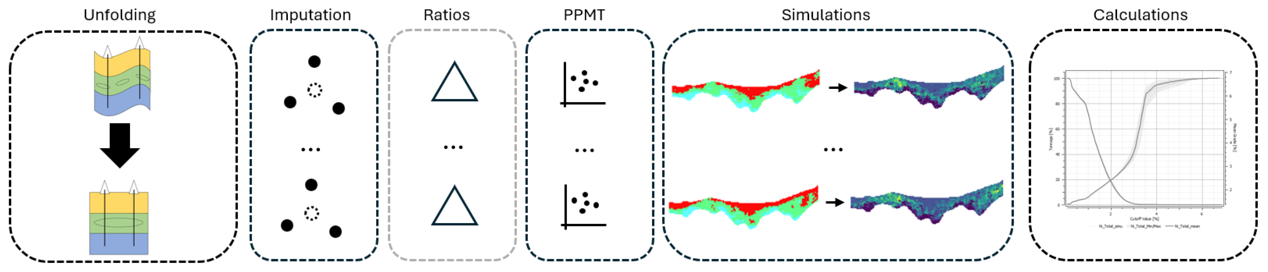
Figure 1. Integrated probabilistic workflow applied in this study for modeling lateritic nickel resources.
Minerals 16 00551 g001
Figure 2. Laterite profile outcrop in East Sulawesi, Indonesia, showing the vertical transition from limonite to saprolite and underlying ultramafic bedrock.
Minerals 16 00551 g002
Figure 3. Three-dimensional view of the dataset showing DDH locations and ERT measurements. Colors represent lithological domains.
Minerals 16 00551 g003
Figure 4. Scatterplot matrix of geochemical variables. Colors indicate lithological domains.
Minerals 16 00551 g004
Figure 5. Comparison between coordinate systems: (a) grid in real-world coordinates; (b) unfolded grid. The topographic surface is represented by a yellow wireframe.
Minerals 16 00551 g005
Figure 6. Data availability for domain SAP: (a) before imputation and (b) after imputation.
Minerals 16 00551 g006
Figure 7. Three-dimensional view of the dataset showing DDH locations. Imputed samples are highlighted in yellow.
Minerals 16 00551 g007
Figure 8. Transition probability matrices used to define the truncation rule: (a) downhole transitions, (b) uphole transitions, and (c) combined transitions.
Minerals 16 00551 g008
Figure 9. PGS Truncation rule.
Minerals 16 00551 g009
Figure 10. Comparison of global lithological proportions from PGS realizations and declustered drillhole data used for validation.
Minerals 16 00551 g010
Figure 11. Three-dimensional view of the conditioning drillholes data and cross-sections for two categorical realizations ((a) realization 1 and (b) realization 2).
Minerals 16 00551 g011
Figure 12. Cross-sections extracted from a realization ((a) realization 1 and (b) realization 2) together with drillhole and ERT data used for validation.
Minerals 16 00551 g012
Figure 13. Variogram reproduction check for Ni in the SAP domain, comparing experimental variograms from simulated realizations with the target variogram model: (a) North–South direction; (b) East–West direction; (c) vertical direction.
Minerals 16 00551 g013
Figure 14. Histogram reproduction check for Ni in the SAP domain, comparing simulated realizations with original sample data.
Minerals 16 00551 g014
Figure 15. Variogram reproduction check for Fe in the SAP domain, comparing experimental variograms from simulated realizations with the target variogram model: (a) North–South direction; (b) East–West direction; (c) vertical direction.
Minerals 16 00551 g015
Figure 16. Histogram reproduction check for Fe in the SAP domain, comparing simulated realizations with original sample data.
Minerals 16 00551 g016
Figure 17. Variogram reproduction check for Co in the SAP domain, comparing experimental variograms from simulated realizations with the target variogram model: (a) North–South direction; (b) East–West direction; (c) vertical direction.
Minerals 16 00551 g017
Figure 18. Histogram reproduction check for Co in the SAP domain, comparing simulated realizations with original sample data.
Minerals 16 00551 g018
Figure 19. Variogram reproduction check for Al in the SAP domain, comparing experimental variograms from simulated realizations with the target variogram model: (a) North–South direction; (b) East–West direction; (c) vertical direction.
Minerals 16 00551 g019
Figure 20. Histogram reproduction check for Al in the SAP domain, comparing simulated realizations with original sample data.
Minerals 16 00551 g020
Figure 21. Variogram reproduction check for MgO in the SAP domain, comparing experimental variograms from simulated realizations with the target variogram model: (a) North–South direction; (b) East–West direction; (c) vertical direction.
Minerals 16 00551 g021
Figure 22. Histogram reproduction check for Mg in the SAP domain, comparing simulated realizations with original sample data.
Minerals 16 00551 g022
Figure 23. Variogram reproduction check for SiO2 in the SAP domain, comparing experimental variograms from simulated realizations with the target variogram model: (a) North–South direction; (b) East–West direction; (c) vertical direction.
Minerals 16 00551 g023
Figure 24. Histogram reproduction check for Si in the SAP domain, comparing simulated realizations with original sample data.
Minerals 16 00551 g024
Figure 25. Scatterplot matrices used for validation of multivariate relationship reproduction. Upper triangles correspond to DDH, and lower triangles to simulated values: (a) in PPMT space prior to back-transformation and (b) after back-transformation.
Minerals 16 00551 g025
Figure 26. Three-dimensional view of the conditioning drillholes data and cross-sections for two Ni realizations ((a) realization 1 and (b) realization 2).
Minerals 16 00551 g026
Figure 27. Cross-sections extracted from a realization ((a) realization 1 and (b) realization 2) together with drillholes.
Minerals 16 00551 g027
Figure 28. Grade–tonnage curves for domain SAP. Simulation-based results are compared with (i) ordinary kriging using deterministically defined domains and (ii) ordinary kriging incorporating proportions derived from indicator kriging.
Minerals 16 00551 g028
Disclaimer/Publisher’s Note: The statements, opinions and data contained in all publications are solely those of the individual author(s) and contributor(s) and not of MDPI and/or the editor(s). MDPI and/or the editor(s) disclaim responsibility for any injury to people or property resulting from any ideas, methods, instructions or products referred to in the content.