
Article

Identification of Geochemical Anomalies by Pattern Recognition: A Case Study of Wulonggou Area in Qinghai Province, China
1
School of Earth Sciences and Resources, China University of Geosciences, Beijing 100083, China
2
Frontiers Science Center for Deep-Time Digital Earth, China University of Geosciences, Beijing 100083, China
3
MNR Key Laboratory for Exploration Theory & Technology of Critical Mineral Resources, China University of Geosciences, Beijing 100083, China
4
Beijing Key Laboratory of Land and Resources Information Research and Development, Beijing 100083, China
5
Development and Research Center, China Geological Survey, Beijing 100037, China
*
Author to whom correspondence should be addressed.
Minerals 2026, 16(4), 411; https://doi.org/10.3390/min16040411
Submission received: 28 January 2026 / Revised: 3 April 2026 / Accepted: 12 April 2026 / Published: 16 April 2026

Abstract

The Wulonggou gold district is located on the northern margin of the Qinghai–Tibet Plateau and represents the most promising area for mineral exploration within the East Kunlun mineralized belt in Qinghai Province. Previous studies on this gold district have lacked a comprehensive assessment of its metal mineralization potential. This paper conducts a comprehensive investigation of the distribution patterns of geochemical data in the Wulonggou gold district, employing multivariate statistical analysis to explore the distribution characteristics of different geochemical elements. Based on the analysis of geochemical anomaly patterns, the median + 2MAD method and fractal method were further introduced to delineate geochemical anomalies. For comparison, machine learning methods—including the radial basis function link network (RBFLN) model and the Bayesian-optimized random forest (BO-RF) model—were also applied to generate different geochemical anomaly maps. By comparing the results obtained from each method, we found that the BO-RF model performed best in predicting geochemical anomalies. Based on the above information, the BO-RF model was integrated with geological background information to delineate prospective areas. These findings provide important clues for mineral exploration and development in the Wulonggou area and can serve as a reference for other regions with similar geological backgrounds.

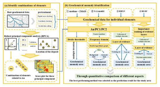
Graphical Abstract

1. Introduction

The formation of a mineral deposit involves a variety of geological processes and their interactions, which give rise to distinctive characteristics that manifest as typical response patterns in geochemical, geological, or geophysical data. These characteristics serve as important diagnostic criteria for deposit identification, yet they also pose significant challenges in prospectivity mapping [1,2]. Geochemical exploration constitutes a key methodology in mineral prospecting, often integrated with multiple data sources to predict mineralization probability and thereby enhance exploration efficiency [3,4,5,6,7,8]. Central to this process is the identification of spatial distribution patterns of geochemical elements and the effective extraction of anomalous signatures [9,10,11]. There are generally two different types of approaches to identifying geochemical anomalies. The first type is methodology based on the analysis of the frequency distribution of the data, such as the frequency distribution method [12,13]. Studies comparing statistical methods for determining geochemical anomaly thresholds have found that the box plot, median ± 2MAD, and empirical cumulative distribution function are more effective than the mean ± 2 standard deviations [14]. This approach to threshold estimation is discussed in detail in Reimann et al. [15]. In addition, the widely used concentration-area (C-A) fractal method in the spatial domain and the spectrum-area (S-A) fractal method in the frequency domain play important roles in geochemical anomaly detection. Other fractal-based methods include local singularity analysis, fractal filtering, and fractal topology [16,17], encompassing but not limited to the concentration-area (C-A) method [18], perimeter-area (P-A) method [19], multifractal inverse distance weighting (MIDW) interpolation method [20], local singularity analysis method [21], and fractal singular value decomposition method [22,23]. These methods have been widely applied [24,25,26]. Notably, in recent years, hybrid approaches based on knowledge-driven or data-driven models have shown promising applications in geochemical anomaly identification and mineral prospectivity mapping. These studies demonstrate the practical value of non-machine learning hybrid models in mineral resource assessment, providing beneficial supplements to the methodological framework for geochemical anomaly detection [27,28].
However, due to the extreme complexity of metallogenic processes and geological activities—such as multi-stage source-transport-accumulation dynamics and intense post-ore modification and overprinting—most traditional geochemical data processing techniques, which are often based on linear assumptions or are empirically driven, exhibit significant limitations when dealing with high-dimensional, non-linear, and noise-affected complex datasets [29,30]. These limitations hinder the effective extraction of deep-seated mineralogical information concealed within the data.
In recent years, machine learning (ML) methods, championed for their data-driven nature and powerful capabilities in non-linear fitting and feature recognition, have been widely introduced into the field of mineral prospectivity mapping (MPM). This paradigm offers a novel approach to addressing the aforementioned challenges [31,32,33,34]. Among the plethora of ML algorithms, decision trees have garnered considerable attention for their model transparency and interpretability. More importantly, ensemble learning methods built upon them, such as Random Forest (RF), have significantly enhanced model generalizability and stability by constructing and aggregating the results of multiple weak classifiers. Consequently, RF has demonstrated remarkable advantages in geochemical anomaly detection [35,36]. The RF algorithm, introduced by Breiman [37] building upon Ho’s [38] random subspace method, ingeniously combines the Bagging ensemble framework with a feature randomization mechanism. This design not only effectively mitigates the overfitting risk inherent in single decision trees but also endows the model with considerable robustness against data noise and missing values. As a result, RF can adapt to diverse and complex exploration scenarios, robustly aggregating the feature discrimination capabilities of multiple trees to provide core support for high-precision geochemical anomaly identification.
Concurrently, as another major class of non-linear modeling techniques, Artificial Neural Networks (ANNs) have seen increasingly profound applications in MPM [39]. ANNs, which simulate the connectivity of neurons in the human brain, can operate as “black-box” models capable of learning and approximating any complex non-linear function. This characteristic makes them particularly suitable for handling the intricate controlling factors in mineral systems. To date, researchers have developed various ANN architectures integrated with Geographic Information System (GIS) techniques for different tasks. These include the Radial Basis Function Linkage Network (RBFLN), noted for its local approximation capability and fast convergence [40]; the Generalized Regression Neural Network (GRNN), suited for continuous variable prediction [41]; and the Probabilistic Neural Network (PNN), which is based on Bayesian decision theory and excels in pattern classification [42,43]. Numerous case studies have demonstrated that these neural network models often achieve predictive performance superior to traditional methods in tackling highly complex, non-linear problems of geochemical anomaly identification and mineral target delineation.
Notwithstanding these advancements, the application of various ML algorithms in MPM continues to face distinct challenges. For instance, while ensemble methods like Random Forest are robust, their “black-box” nature complicates geological genesis interpretation [5,44]. Conversely, neural network models are often highly sensitive to hyperparameter configuration and typically require large sample sizes to ensure effective training, thus limiting their application in data-scarce regions. Therefore, a central focus and critical frontier of current research in this field lies in fully leveraging the strengths of different algorithms while effectively overcoming their inherent limitations, and further exploring their deep integration with geological metallogenic theory.
This study conducts a comparative analysis of results obtained from different data processing methods within the same region, aiming to identify an appropriate integrated methodological approach for the area. By combining multiple geochemical anomaly identification methods, the proposed framework ultimately achieves the stated objectives of this research: to explore the mineral exploration potential within the study area and to provide support for the ongoing efforts in prospecting target delineation in the Wulonggou area.

2. Study Area

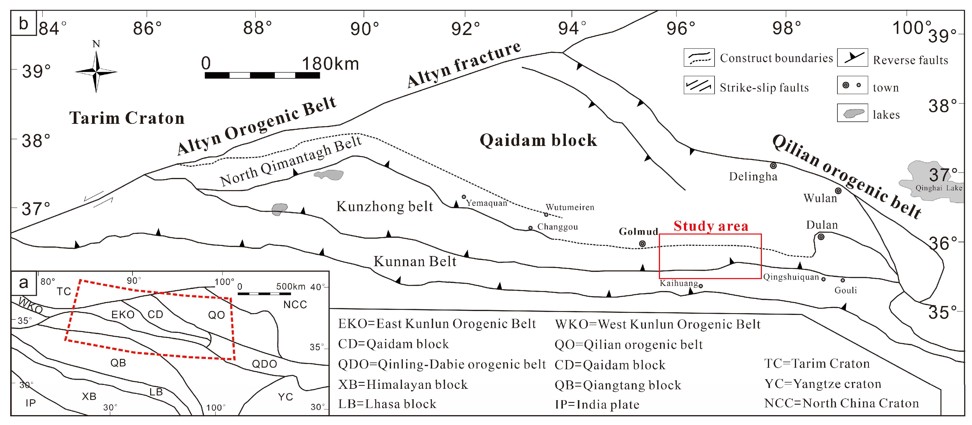
The study area is situated within the Kunlun Mountains, specifically in the Wulonggou-Nuomuhong region of Dulan County, Qinghai Province, along the eastern margin of the Qinghai–Tibet Plateau. Tectonically, the region lies within the East Kunlun orogenic belt, positioned on the northern edge of the Qinghai–Tibet Plateau. It is bounded to the south by the Kunnan Fault, which separates it from the Bayankala Block, and to the north by the Hongliuquan-Golmud Fault, demarcating its boundary with the Qaidam Block. The regional tectonic framework is illustrated in the figure below (Figure 1).
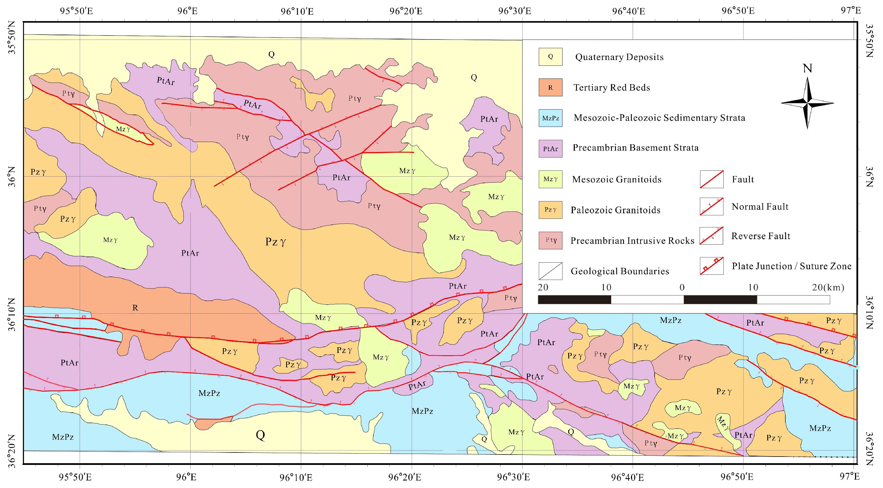
Geologically, the study area exhibits stratigraphic development from the Paleoproterozoic to the Cenozoic, with the Proterozoic and Triassic formations being the most prominent. Strata from other periods, ranging from the Carboniferous to the Quaternary, are also exposed to varying extents (Figure 2). Notably, NWW-trending (north–northwest-trending) faults are highly developed within the area. The East Kunlun Orogenic Belt has undergone several distinct geological stages, establishing itself as a typical multi-cyclic composite orogenic belt spanning from the Late Neoproterozoic to the Early Paleozoic, the Late Paleozoic to the Early Mesozoic, and into the Mesozoic era. Of particular significance are the orogenic events between the Late Paleozoic and Early Mesozoic, which are closely associated with the formation of large-scale gold deposits in the East Kunlun region [45].
During the Late Permian, the Paleo-Tethys Ocean initiated northward subduction, culminating in the Middle Triassic with the collision and amalgamation of the Kunnan and Kunzhong Belts, which formed a series of tectonic mélange zones [36,46]. The geological processes during this stage influenced the migration of ore-forming fluids and the localization of ore bodies. Ultimately, tectonic-magmatic activities associated with the Indosinian/post-collisional orogeny facilitated the accumulation of large-scale gold deposits, playing a decisive role in the formation of the metallogenic environment in the Wulonggou region [47].

3. Methodology

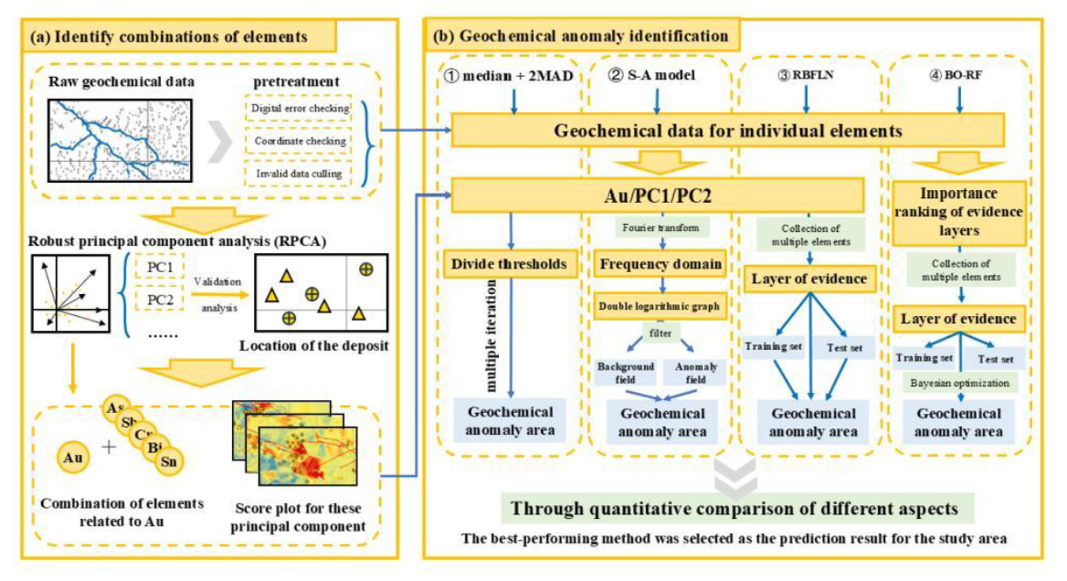
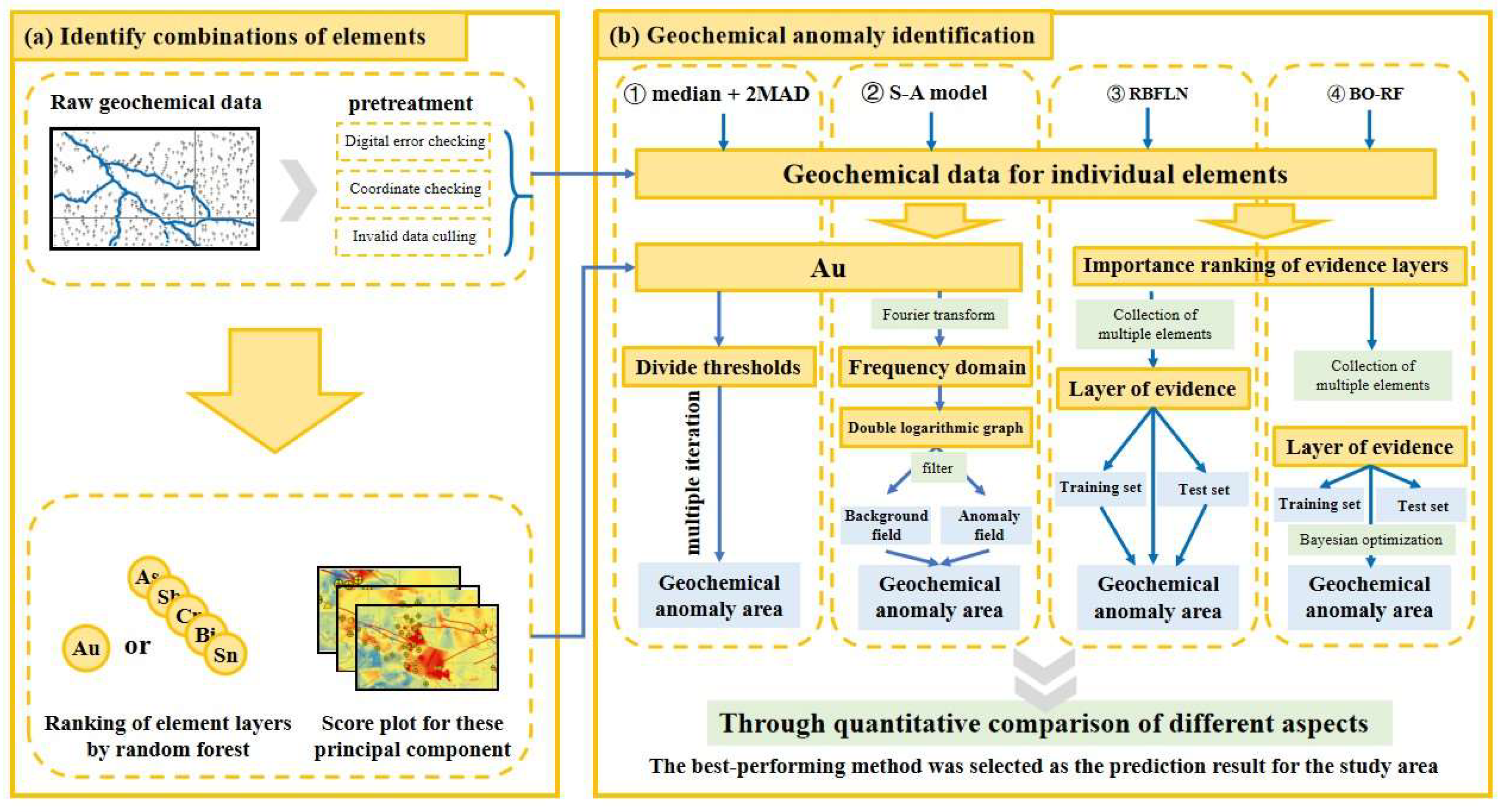
Based on the analysis of geochemical data distribution patterns, this study preprocessed the stream sediment geochemical data and employed the centered log-ratio (clr) transformation to eliminate the closure effect. Multiple thresholding methods (such as median + 2MAD and fractal analysis) were combined to delineate geochemical anomalies. Furthermore, two machine learning models—the radial basis function link network and the Bayesian-optimized random forest—were introduced for anomaly prediction and comparison to determine the optimal prediction method. Finally, by integrating the results of the optimal machine learning model with geological background information, prospective exploration areas in the study region were comprehensively delineated. The technical route is illustrated in Figure 3.

3.1. Centered Log-Ratio Transformation for Compositional Data

Geochemical data are inherently compositional—element concentrations sum to a constant (e.g., 100% or 106 ppm)—which induces the closure effect and renders conventional statistical analyses based on Euclidean geometry invalid [48,49]. To eliminate this closure effect and map the data from the simplex space to real Euclidean space, log-ratio transformations are required.
Among various log-ratio transformations, the centered log-ratio (clr) transformation is particularly useful for subsequent multivariate analysis because it preserves all original variables. Following Egozcue et al. [50], for a D-part composition x = (x1, …, x_D)T, the centered log-ratio (clr) transformation is defined as:
c l r ( x ) = ( y 1 , , y D ) = ( l n ( x 1 / g ( x ) ) , , l n ( x D / g ( x ) ) )
where g(x) = ᴰ√(x1·x2·…·xᴰ) is the geometric mean of the parts across the composition.
The clr-transformed data are free from the constant sum constraint and map the composition from the simplex to a D-dimensional real Euclidean space. However, the clr coefficients satisfy the linear constraint y1 + y2 + … + yD = 0, which results in a singular covariance matrix. Despite this singularity, the clr transformation preserves all original variables and allows for straightforward interpretation of the relationships between individual parts.
The transformation can be written equivalently in vector form as:
Y   =   V   In ( x )
where V   =   I D 1 D J D is the centering matrix, with ID being the D × D identity matrix and JD the D × D matrix of ones.
The resulting clr coefficients are free from the closure effect, providing a suitable foundation for subsequent statistical analysis and the application of various methods.

3.2. Geochemical Anomaly Identification

3.2.1. Absolute Median Difference

Hawkes [51] proposed using the mean + 2 standard deviations (mean + 2STD) method to determine the threshold for geochemical element anomalies in relatively large geochemical datasets. However, this method requires the data to conform to a normal distribution, and the iterative culling process may lead to the loss of valid information. Therefore, this paper adopts the median + 2 median absolute deviation (median + 2MAD) method as an alternative to the traditional mean + 2STD method. The median absolute deviation (MAD) is defined as the median of the absolute deviations from the overall data median [52], and is calculated as MAD = median(|xi − median(X)|). This method is based on the actual distribution characteristics of the data, utilizing the median as a location parameter instead of the mean, and MAD as a scale parameter instead of the standard deviation. Given that the median is insensitive to extreme values and that MAD is constructed based on the median, both exhibit robust statistical properties. Consequently, the median + 2MAD method can undergo statistical testing without relying on assumptions of normality, independence, or identical distribution. It effectively reduces the impact of abnormally high values on threshold determination and demonstrates enhanced robustness and adaptability in the processing of geochemical data that are non-normally distributed or contain outliers.

3.2.2. Fractal Method

The proposed elemental content-area method (C-A) model [18].
A ( ρ   >   c )   =   c β
where A(ρ > c) denotes the region where the element content (ρ is the concentration) exceeds a certain threshold. The threshold c is determined by the singularity exponent β, and the specific form of this transformation is given in Equation (4).
A ( ρ >   c )   =   K c β
Equation (5), take the natural logarithm on both sides:
l n ( A ( ρ > c ) )   =   β l n ( c ) + l n ( K )
The area with a content greater than a certain value is linearly related to this threshold in a double logarithmic coordinate system, and the slope of the straight line in this linear relationship is the fractal dimension. Since the geochemical element distribution satisfies the multifractal power-law distribution, the same element will present a multilinear relationship in double logarithmic coordinates, indicating the existence of multiple fractal dimensions. The piecewise linear fitting of the double logarithmic scatter plot by the least squares method was used to find out the element content value corresponding to the intersection of the two straight lines, which was the lower limit of the anomaly of the element in the area.
Furthermore, in the identification of anomalies in historical geochemical data, the geological processes causing the anomaly differ from those contributing to the geochemical background, and the geochemical measurements reflect only the superimposed and combined results of both [18,53]. Thus, the spectrum-area (S-A) fractal method transforms geochemical data from the spatial domain to the frequency domain using the Fourier transform. It then decomposes the distribution of generalized self-similar features into distinct filters in the frequency domain, and finally, the inverse Fourier transform is applied to return the data to the spatial domain, enabling the separation of anomaly and background fields. This approach, referred to as the spectrum-area (S-A) fractal model, is based on the generalized self-similarity principle proposed by Cheng [54]. The S-A model is represented by the following formula:
A ( S )   S β
where S represents the spectral density, A ( S ) denotes the area where the spectral density exceeds S in the spectral density space, and β is the fractal dimension determined via least-squares fitting of each line segment. The inverse Fourier transform is then applied to convert the filtered results from the frequency domain back to the spatial domain, using the following formula:
B   =   F 1 ( F ( T ) G B ( ω ) )
A   =   F 1 ( F ( T ) G A ( ω ) )
C   =   F 1 ( F ( T ) G C ( ω ) )
where F and F 1 represent the Fourier transform and inverse Fourier transform, respectively. These formulas are used to construct high-pass, low-pass, and band-pass filters.

3.2.3. Radial Basis Functional Link Networks (RBFLN)

The radial basis function neural network (RBFNN) model, proposed by Lowe in 1988, is capable of handling complex nonlinear spatial datasets [55,56]. This model can process these datasets and be trained using both known deposits and non-mineral deposits to identify relationships between training points and evidence graphs. The RBFLN model is designed to process complex nonlinear spatial datasets [55]. It consists of a three-layer feedforward structure comprising an input layer, a hidden layer, and an output layer. The model uses known mineral and non-mineral deposits as training samples [57,58] classify unknown points [12,59].
The structure consists of an input layer with N nodes that receive the input eigenvector x, and a hidden layer with M neurons. Each neuron in the hidden layer processes the input eigenvector x and outputs a value y. If x q is provided as input to the mth neuron, the output value y m q is given by [60]:
y m q = e [ x q v m 2 / 2 σ m 2 ] , 0 < y 1
Here, x q denotes the eigenvector of the nth input, v m represents the center of the nth RBF function in the hidden layer—corresponding to the maximum likelihood point of the RBF function—and σ m represents the width or spread of the nth neuron [2,58]. Thus, the output value of the RBF function is higher when the input eigenvector is closer to the center, and decreases monotonically as the distance between the input eigenvector and the center increases.
In this paper, each node in the input layer corresponds to a cell in the unique conditional raster data, where each cell’s data is represented by an n-dimensional feature vector X ( x 1 , x 2 , , x n ) after appropriate filtering, where n is the number of geochemical variables (elements) considered. The hidden layer consists of M artificial neurons modeled by RBF functions. Each neuron in the hidden layer processes the input feature vector X and returns Y as the output, which is multiplied by the synaptic weight between the hidden and output layers.
The sum of squares of error (SSE) between the output vector z and the target vector t is defined as:
S S E   =   q = 1 Q j = 1 J ( t j q z j q ) 2
The SSE quantifies the error between the target vector T and the output vector Z, serving as an important metric for evaluating the performance of the model.

3.2.4. Random Forest Model Based on Bayesian Optimization (BO-RF)

Random Forest (RF) is an ensemble learning algorithm proposed by Breiman, designed to enhance the accuracy and stability of decision tree models [37]. This algorithm integrates subspace partitioning, stochastic decision tree generation, and optimal segmentation theory. It generates multiple sample subsets from the original training set via bootstrap sampling to construct individual decision trees, thereby producing multiple weak classifiers. The final prediction is obtained by aggregating the results of these weak classifiers through voting or averaging. This mechanism effectively mitigates the overfitting risk associated with single decision trees and improves the model’s generalization capability. Specifically, RF combines the bagging algorithm with random feature selection. During the construction of each decision tree, it not only randomly samples the data but also randomly selects a subset of features, introducing dual randomness into the training process. This enhances the diversity among models, making the ensemble classifier more robust. The complete random forest algorithm typically involves three key stages: evaluation and selection of feature importance, parallel construction of multiple decision trees, and final decision-making based on ensemble strategies.
To improve the model’s performance on specific datasets, this study introduces the Bayesian Optimization (BO) algorithm to automatically tune the hyperparameters of the random forest. Bayesian optimization is a sequential model-based global optimization method. It utilizes prior knowledge and observations of the black-box objective function to iteratively approximate its posterior distribution. Specifically, the algorithm first constructs a probabilistic surrogate model based on existing hyperparameter combinations and their corresponding model performances. It then employs an acquisition function to balance exploration and exploitation within the hyperparameter space, selecting the next most promising hyperparameter combination for evaluation [61]. Upon obtaining each new set of observations, the surrogate model is updated to approximate the true distribution of the objective function more accurately. This iterative process continues until the hyperparameter configuration that optimizes the objective function is found. To approximate the true objective function more precisely, the Bayesian optimization algorithm in this study employs Gaussian processes as the surrogate model. Gaussian processes provide uncertainty estimates for predictions, which is crucial for balancing exploration of unknown regions and exploitation of known optimal areas. The mathematical expression for parameter optimization is as follows:
X *   =   a r g m a x x X f ( x )
where x represents the hyperparameter combination to be optimized, X is the hyperparameter search space, and f(x) is the objective function fitted by the surrogate model (e.g., AUC value after cross-validation). The optimization objective is to find the x that maximizes f(x).
In summary, the BO-RF algorithm adopted in this study follows a systematic optimization workflow:
Step 1: Define Hyperparameter Space: First, based on the characteristics of the random forest algorithm and the specific requirements of the research problem, the range of hyperparameters to be optimized is defined. This includes, but is not limited to: the number of trees (n_estimators), maximum tree depth (max_depth), minimum number of samples required to split an internal node (min_samples_split), minimum number of samples required at a leaf node (min_samples_leaf), and the maximum number of features considered for splitting (max_features).
Step 2: Select Objective Function: The evaluation metric guiding the optimization process, i.e., the objective function, is defined. The input to this function is the hyperparameters defined in the first step, and the output is the metric used to measure model performance. In this study, considering the balance in classification problems, the AUC value is chosen as the output of the objective function because AUC provides a comprehensive evaluation of the model’s ability to distinguish between positive and negative samples.
Step 3: Initialization and Iterative Optimization: At the beginning of optimization, several hyperparameter combinations are randomly selected to evaluate the objective function, serving as initial observation points. Subsequently, the BO algorithm enters an iterative loop: Based on all current observation points (known hyperparameter-performance pairs), the Gaussian process surrogate model is updated; according to the predicted mean and variance from the surrogate model, an acquisition function (e.g., Expected Improvement, EI, or Upper Confidence Bound, UCB) is constructed and optimized to determine the next hyperparameter combination most worthy of evaluation; this newly selected combination is then used to train the RF model and compute its AUC value on the validation set, and this result is added as a new observation point to the historical dataset.
Output Optimal Configuration: Step 3 is repeated until a preset number of iterations or a performance convergence threshold is reached. Finally, the algorithm outputs the hyperparameter combination that achieved the optimal objective function value during the search process. This configuration is considered the optimal setup for the BO-RF model and is subsequently used for final model training and anomaly identification tasks.

4. Results and Discussion

4.1. Analysis of the Characteristics of Data

First, all geochemical data underwent preprocessing, including data quality inspection (such as coordinate verification and duplicate point removal). After using histograms for preliminary data statistics to remove elements with an excessive concentration of zero values, normalization was applied to the remaining eligible element data. This study subsequently focused on the characteristic values of 17 elements, including Au, Ag, Sn, As, Sb, Bi, Hg, Pb, Zn, V, W, Mo, Cd, Cr, Ni, Co, and Fe (Table 1).
The results indicated that the elements with enrichment coefficients greater than 1 in the study area’s soils were Au, Sn, As, and Sb, while the remaining elements were classified as weakly enriched. The coefficient of variation for Au exceeded 1.5, suggesting an extremely uneven distribution and strong activity and migration capabilities. In contrast, the coefficient of variation for Bi ranged between 1.0 and 1.5, indicating an uneven distribution with relatively strong activity and migration capabilities. For the other elements, the coefficients of variation were less than 1.0, signifying weak activity and migration abilities.
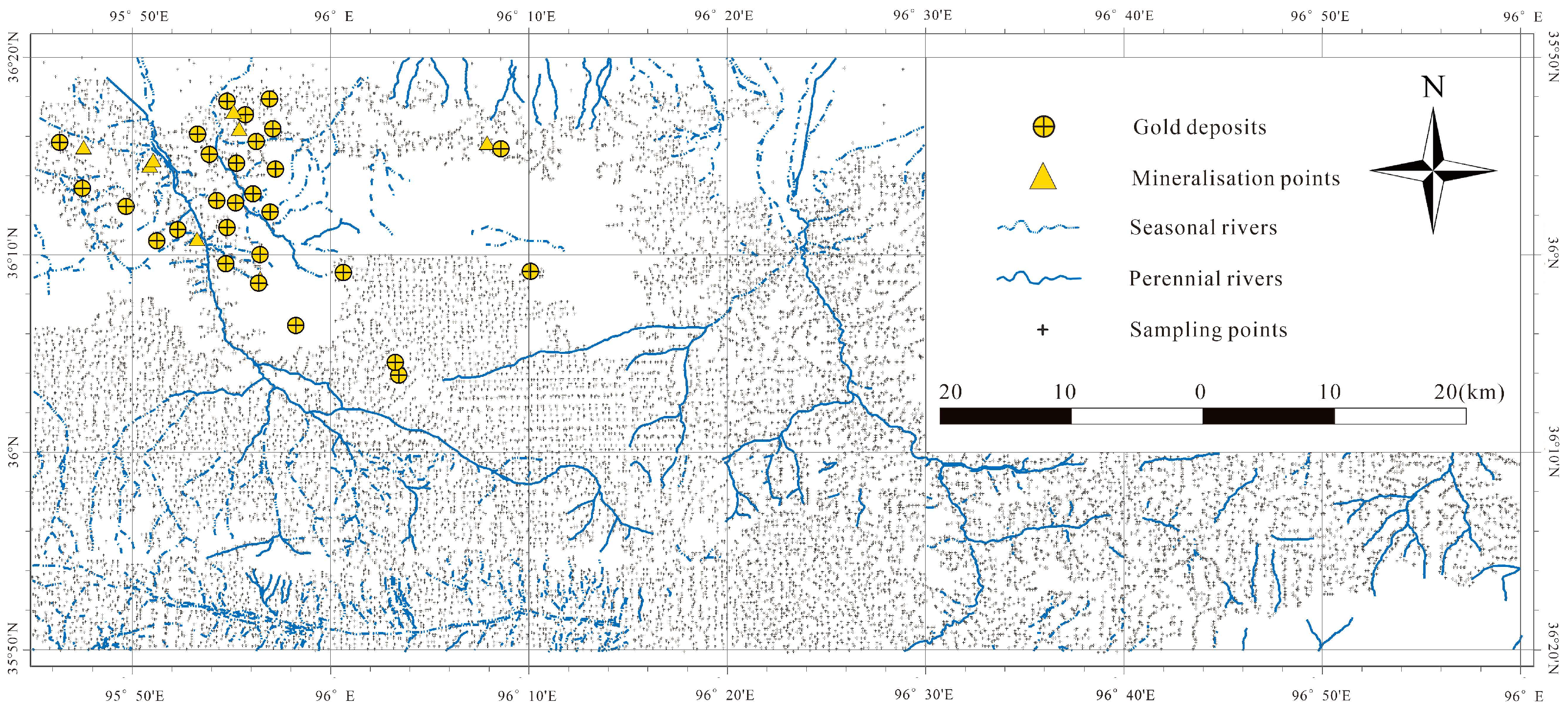
After verifying the coordinates of the original data for numerical errors and duplicate points, invalid data were eliminated, resulting in a final valid dataset of 17,599 samples, as illustrated in Figure 4.
In this study, the data were first standardized. Subsequently, to address the inherent closure effect in geochemical data, the centered log-ratio transformation was applied. Furthermore, mandatory closure correction was performed on the geochemical data for each sample following the approach of Aitchison [62].

4.2. Geochemical Anomaly Pattern Recognition

4.2.1. Absolute Median Difference

This study employs the median plus two times the median absolute deviation (MAD) method to analyze the Au element content values. This approach is based on the actual distribution characteristics of the data and, compared to the traditional mean ± 2 standard deviations method, is less affected by extreme outliers, enabling more robust identification of geochemical anomalies. The calculated median + 2MAD value serves as the lower threshold for geochemical anomalies, effectively distinguishing between the background field and the anomalous field. Building upon this, the concept of multiples length is introduced. Using this threshold as a baseline, anomaly intensity intervals are divided according to a geometric progression, with the double frequency length of each anomaly determining the length of subsequent segments. This allows for refined classification of the inner, intermediate, and outer zones of the anomalies, as illustrated in Figure 5.
First, all geochemical data underwent preprocessing, including data quality inspection (such as coordinate verification and duplicate point removal), outlier identification and removal, missing value imputation, and data normalization. After removing elements with values approaching zero, this study focused on the characteristic values of 17 elements, including Au, Ag, Sn, As, Sb, Bi, Hg, Pb, Zn, V, W, Mo, Cd, Cr, Ni, Co, and Fe (Table 1). Furthermore, given that ore prospecting represents an extremely low-probability event in nature, both known mineral deposits and known mineralized occurrences in the study area were selected as positive samples in this paper.

4.2.2. Fractal Method

The distribution of various chemical elements in nature is highly heterogeneous, and the complexity of mineralization processes further exacerbates the uneven distribution of geochemical elements. Consequently, quantifying metallogenic complexity and elucidating ore-forming mechanisms have become significant research priorities in mineral deposit studies. In this paper, C-A fractal analysis was initially attempted on sample data interpolated using the Inverse Distance Weighting (IDW) method. However, given that the study area has been affected by multi-stage tectonic movements and mineralization events (such as intrusive activities in the region), weak anomalies in low-background fields are often suppressed, making them difficult to detect effectively using traditional univariate or multivariate anomaly identification methods. In contrast, the S-A fractal filtering technique comprehensively accounts for the anisotropy, generalized self-similarity, and scale invariance of geochemical fields, enabling effective identification of subtle and latent anomalies. Therefore, this study applies the S-A fractal filtering technique for the specific purpose of anomaly recognition and decomposition for the Au element.
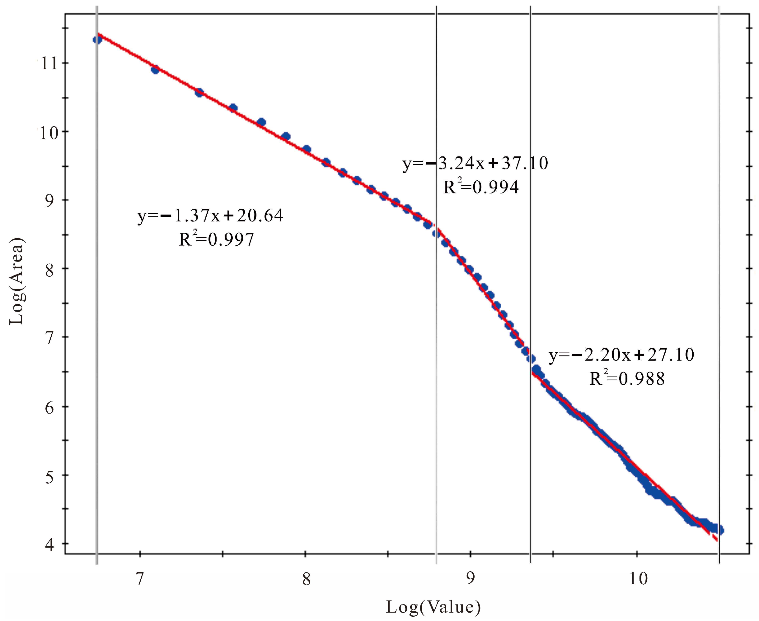
First, the S-A fractal filtering technique was applied to the Au element using GeoDAS 4.0. This method transforms geochemical data from the spatial domain to the frequency domain via the Fourier transform to obtain the power spectrum density. In the S-A fractal model, the power spectrum density value (value) and its corresponding area (Area), i.e., the area enclosed by the number of frequencies with a power spectrum density greater than a given value, follow a power-law relationship. A scatter plot is constructed on a log-log coordinate system, where the horizontal axis represents the logarithm of the power spectrum density (log(value)), and the vertical axis represents the logarithm of the cumulative area (log(area)). The power spectrum density value is calculated using the formula:
v a l u e   =   | F ( u , v ) | 2
where F(u,v) is the two-dimensional Fourier transform of the geochemical data grid. If the data exhibit piecewise linear characteristics, it indicates the presence of distinct generalized self-similar structures corresponding to different geological processes (such as background fields, noise fields, and anomaly fields). The distribution of gold content clearly conforms to fractal characteristics, making it suitable for fitting a three-segment straight line using the least squares method. The results indicate that the R2 values for each segment remain around 0.90, demonstrating a strong goodness of fit (Figure 6). The slopes of the three segments are −1.37 (corresponding to the noise field), −2.20 (corresponding to the background field), and −3.24 (corresponding to the anomaly field). Accordingly, the values corresponding to the inflection points were used as thresholds for the filter, categorizing the data from left to right into noise fields, background fields (Figure 7), and anomaly fields (Figure 8).
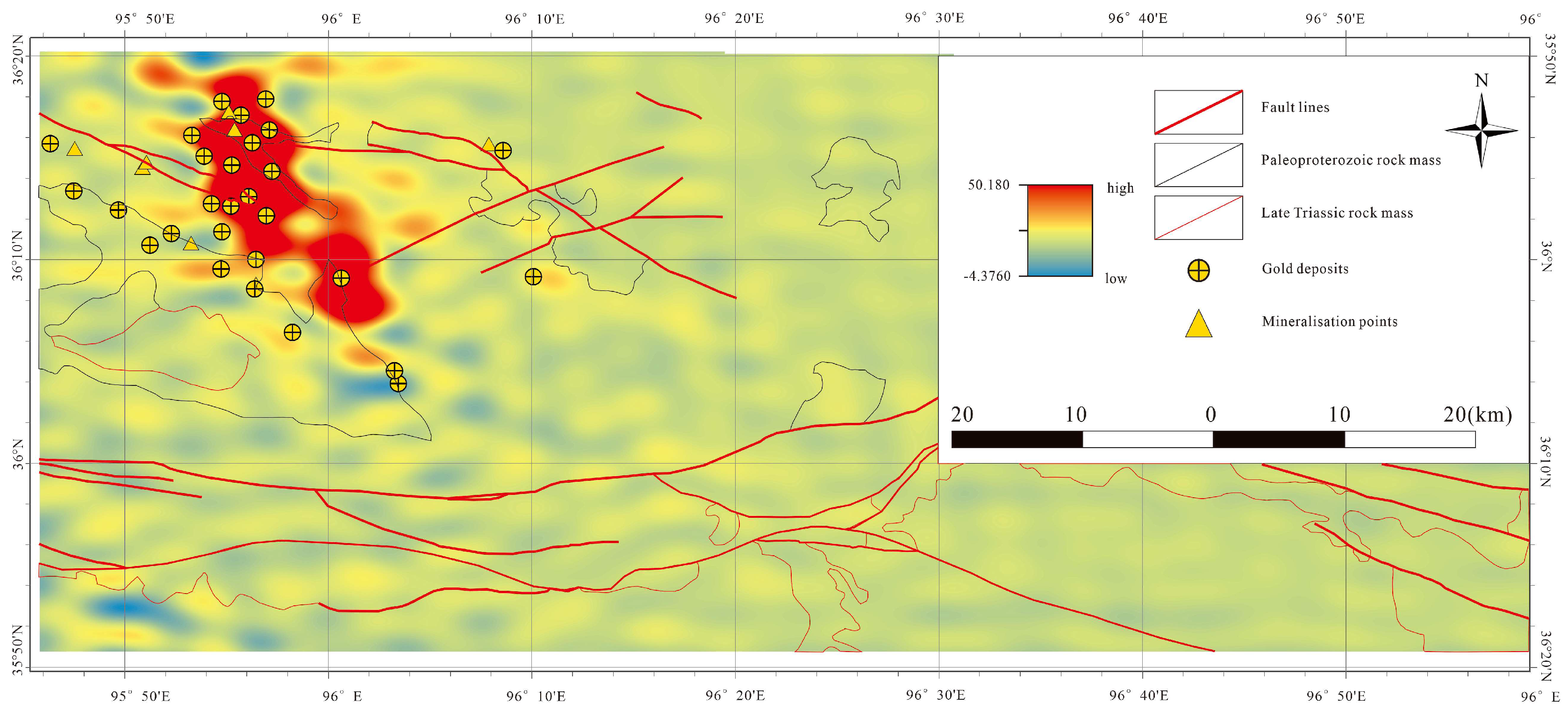
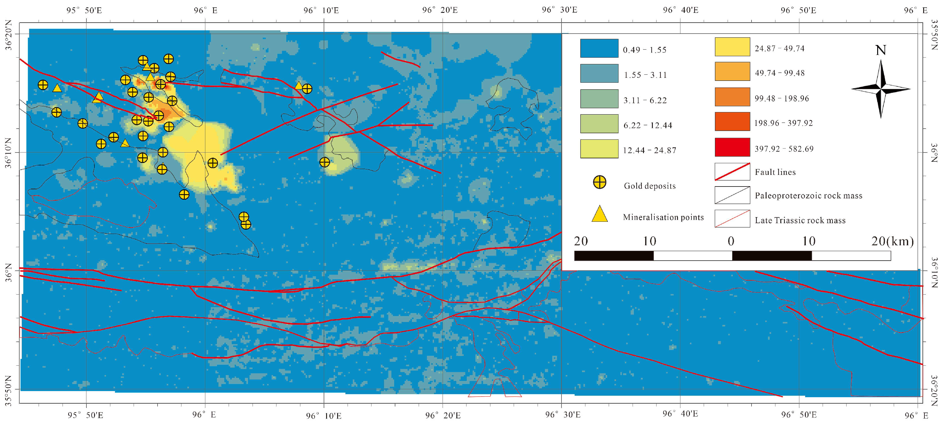
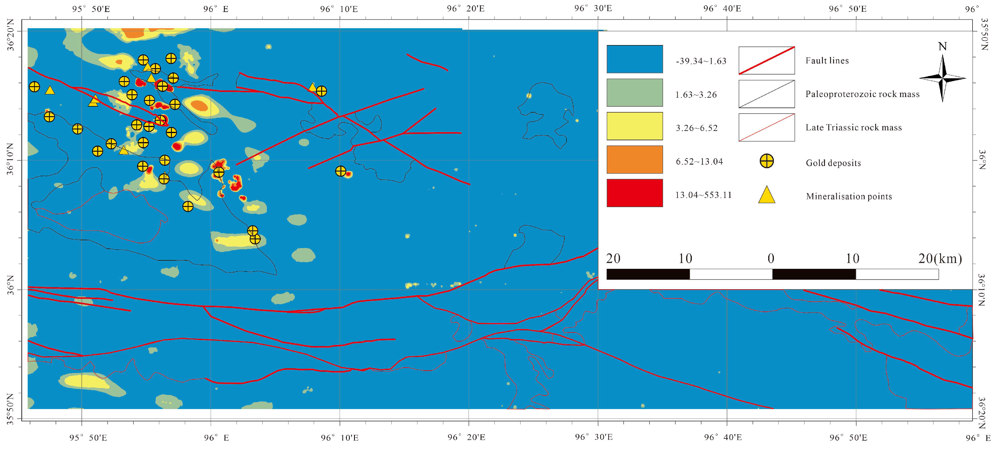
In the background field (Figure 7), the favorable geological environment for gold mineralization in the study area is clearly highlighted. The identified deposits are concentrated within high-background zones, which align with the trends of the main faults and strata oriented in a NWW direction. A distinct high-value area is observed in the northwestern corner.
In Figure 8, the median method was employed to determine the threshold for the Au element anomaly field, followed by classification to delineate the anomaly extents. This approach effectively identified several localized anomalies exhibiting spotted and bead-like patterns, which exhibit a close spatial relationship with the distribution of known mineral deposits.

4.2.3. Radial Basis Functional Link Networks (RBFLN)

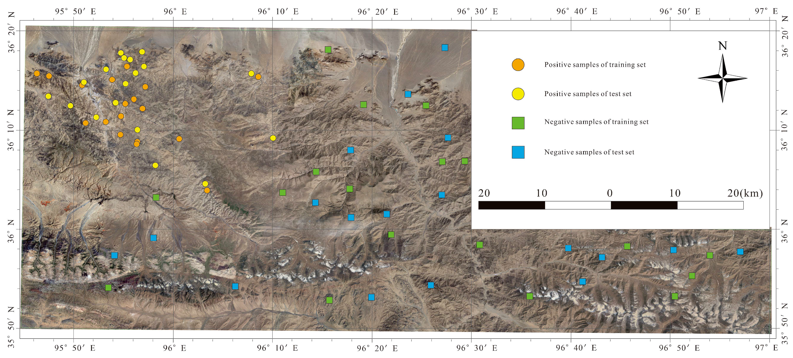
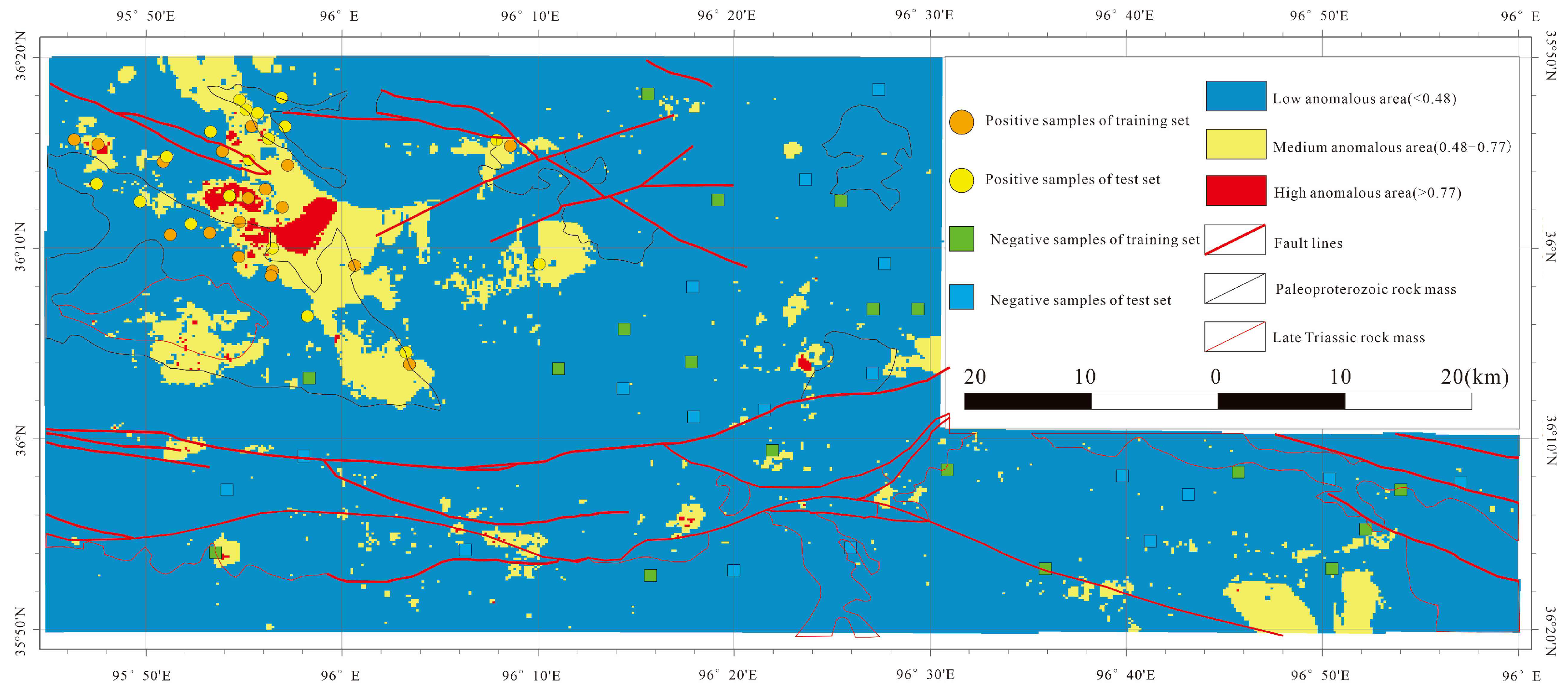
This study utilizes GeoXplore 5.1 and ArcGIS 10.8, employing ArcSDM [63] as a component of the GIS data processing tools to implement the RBFLN algorithm for constructing a geochemical anomaly identification model. To effectively train the model and evaluate its classification performance, 24 of the 36 known gold mineral occurrences in the study area were selected as positive training sample points, with the remaining 12 occurrences serving as positive test sample points. The negative sample points (i.e., non-mineralized points) were selected using a randomized dispersion strategy and uniformly distributed throughout the study area. This approach aimed to maximize the acquisition of background geochemical information while strictly ensuring no overlap with known mineralized points and favorable metallogenic zones, thereby avoiding sample selection bias and ensuring that the negative samples accurately represent non-mineralized backgrounds. Considering the area of the study region, the complexity of its geology, and the number of positive samples, 12 negative training samples and 12 negative test samples were ultimately selected, with their spatial distribution illustrated in Figure 9. This sample configuration provides a foundation for achieving a balance between positive and negative samples and for the effectiveness of subsequent model training.
It should be noted that the machine learning models employed in this study (RBFLN and BO-RF) were trained and evaluated on a relatively small dataset. Due to the spatial nature of geochemical data, a single training/test sample split may have an impact on the performance evaluation, and the models are somewhat sensitive to specific training data combinations. Although this limitation does not substantially affect the cross-model comparison between the two algorithms, future research could enhance the robustness of the evaluation results by introducing robustness tests such as repeated random splits, thereby further validating the models’ generalization capability and providing a more comprehensive interpretation of evaluation metrics such as AUC values.
Based on the results of element feature importance ranking using the Random Forest algorithm, this study extracted the top eight elements associated with gold mineralization (Ag, Sb, Pb, Sn, Cd, Hg, As, V) as geochemical evidence layers for RBFLN model training.
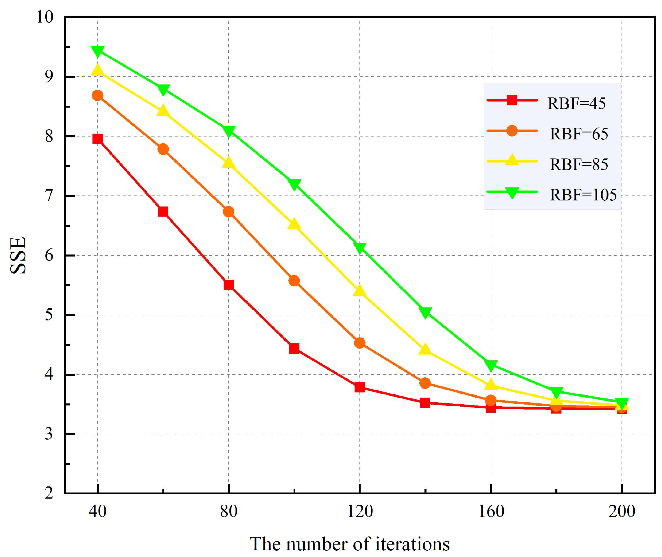
The RBFLN training process requires determining two key parameters: the number of radial basis functions and the number of iterations, optimized to minimize the sum of squared errors (SSE) between model outputs and target vectors. Through systematic experimentation with radial basis function quantities (45, 65, 85, 105) at intervals of 20 and iteration counts ranging from 40 to 200 in increments of 20, we observed that the SSE gradually decreased with increasing iterations and asymptotically approached zero, though never exactly reaching it (Figure 10).
However, models exceeding 160 iterations demonstrated over-learning behavior leading to overfitting. As noted by Porwal et al. [64], overfitted models achieve perfect classification on training features but lack generalization capability. Therefore, models with iterations beyond 160 were excluded. During training, synaptic weights were iteratively adjusted through self-organization to minimize prediction error. The weight adjustment process, expressed as a function of the error between output (z) and target (t), continued through multiple iterations until specified limits were reached.
Consequently, we selected hyperparameters that both prevent overfitting (iterations ≤ 160) and minimize the sum of squared errors. The optimal configuration was determined to be 140 iterations with 45 radial basis functions (Figure 10).
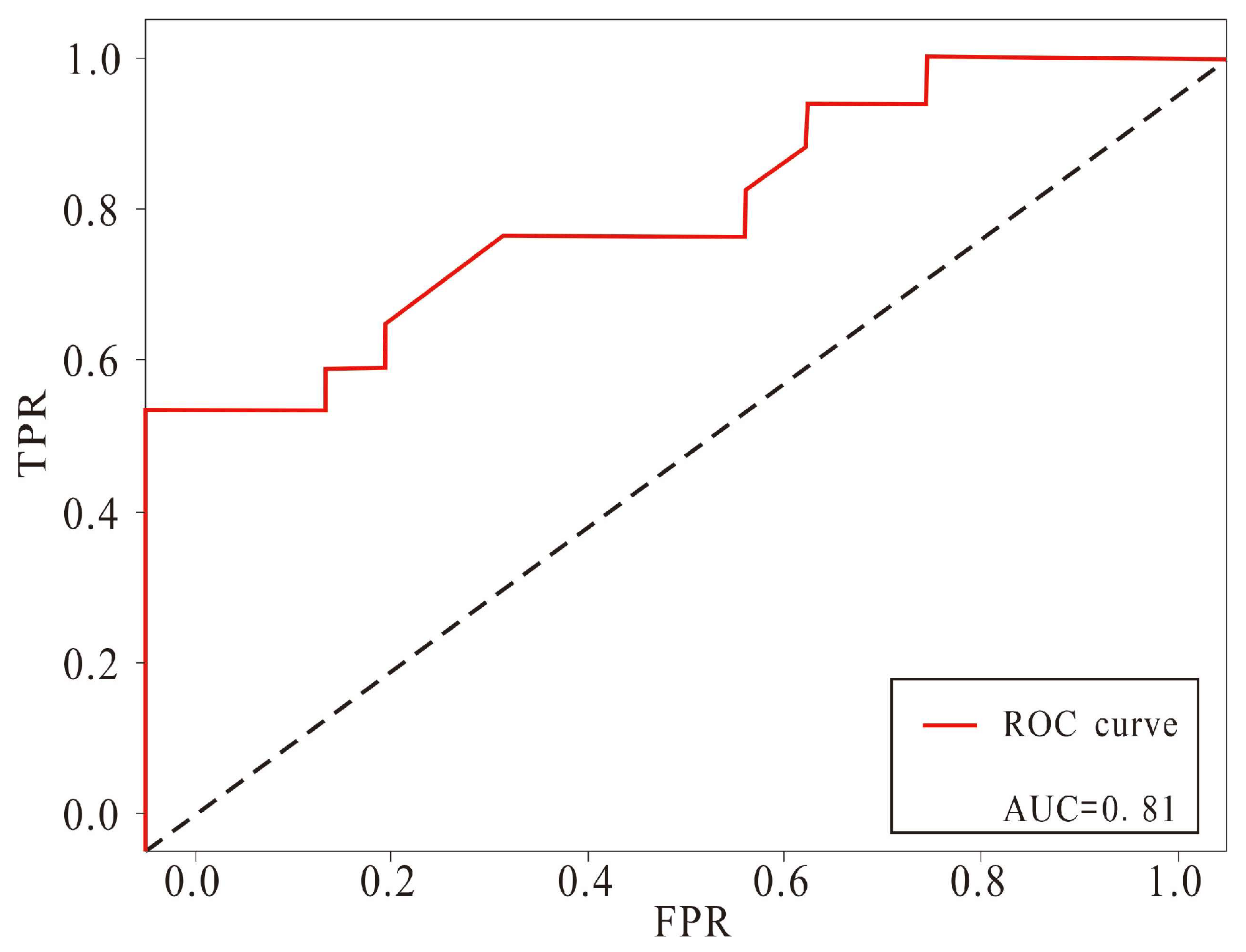
The trained model’s capability to classify unknown feature vectors into positive/negative categories was evaluated using the test dataset, achieving an AUC value of 0.81 in ROC analysis (Figure 11), indicating satisfactory classification performance.
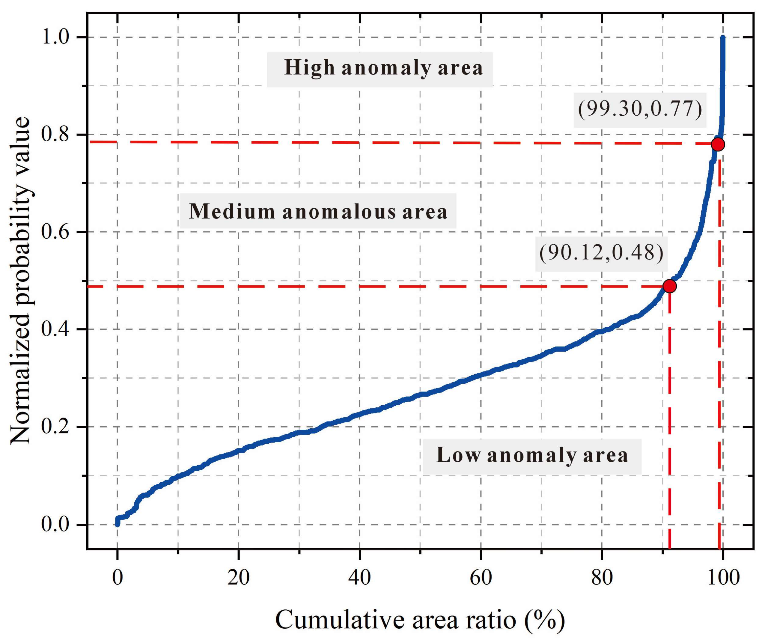
Finally, to illustrate the obtained mineral prospectivity map, the RBFLN probability output was normalized and plotted to create a regional cumulative percentage map, with (90.12, 0.48) and (99.30, 0.77) used as the separation points between the low-probability and medium-probability zones, and between the medium-probability and high-probability zones, respectively (Figure 12). The study area was classified into high-, medium-, and low-probability zones for mineralization potential (Figure 13).

4.2.4. Random Forest Algorithm Based on Bayesian Optimization

This study implements the BO-RF algorithm model using Python 3.11, trained with the same training and testing datasets as those used for RBFLN. The core parameters were initially configured, establishing a preliminary model. Preliminary evaluation employed metrics including AUC, accuracy, recall, F1 score, and precision. These metrics collectively assess the model’s classification capability, with AUC specifically serving as a measure of overall performance in distinguishing between positive and negative samples. Therefore, AUC was selected as the primary evaluation criterion for subsequent model training in this study.
Subsequently, a preliminary analysis of feature importance across multiple input evidence layers was performed, generating a feature importance ranking diagram that illustrates the contribution of each layer to model predictions. Eight elements (Ag, Sb, Pb, Sn, Cd, Hg, As, V)—the same element layers selected for the RBFLN algorithm—were utilized as evidence layer inputs for training. The optimal hyperparameter combination yielding the highest AUC value was identified and incorporated into the Random Forest model for subsequent analysis. Following Bayesian optimization of model parameters, the final optimized Random Forest model was employed to predict the deposit occurrence probability for each raster cell, generating a predictive probability grid across the study area and ultimately producing a raster file of prediction probabilities.
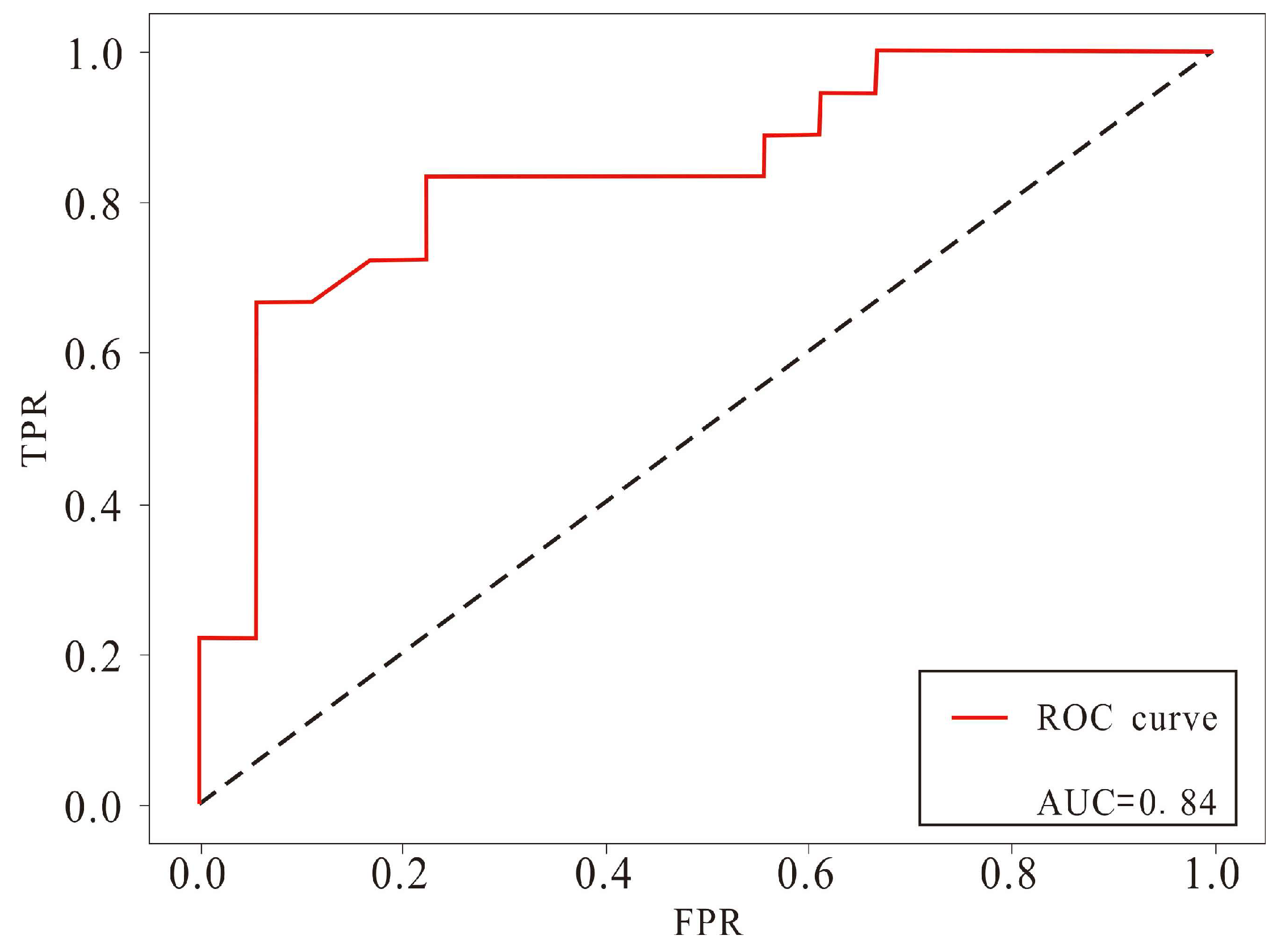
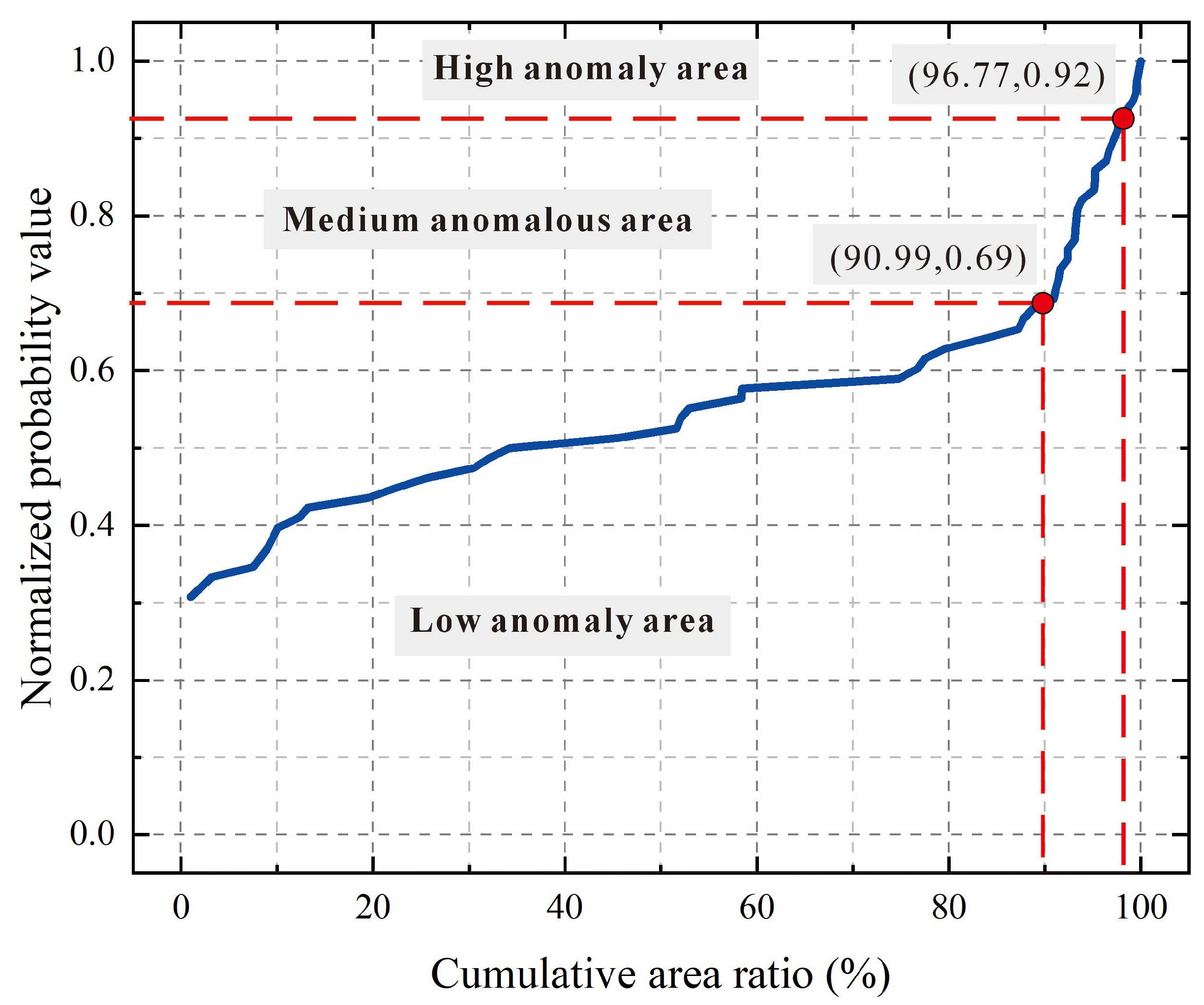
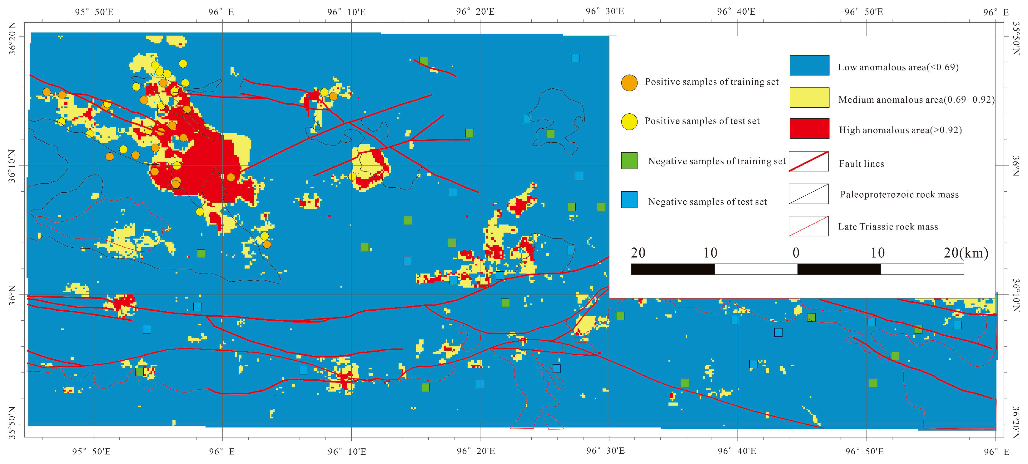
Furthermore, ROC curve analysis was conducted to evaluate the model’s classification accuracy. The results demonstrated an AUC value of approximately 0.84, indicating the classifier’s competent performance in distinguishing between positive and negative samples (Figure 14). Finally, based on fractal theory, the cumulative percentage distribution of probability values within the study area was analyzed, and two reasonable breakpoints were determined to be 90.99% and 96.77% of the cumulative area, with corresponding normalized probability values of 0.69 and 0.92, respectively. This divided the graph into three intervals with different scale patterns (Figure 15). This approach enabled an objective delineation of high, medium, and low mineral potential zones, thereby generating a mineral prospectivity map with three distinct classification zones (Figure 16).
The described procedure demonstrates that the Bayesian-optimized Random Forest model (BO-RF) effectively enhances prediction accuracy by providing an optimally parameterized model for mineral probability prediction. This enables more precise determination of mineralization probabilities at different pixel locations and consequently delineates more accurate mineral prospectivity distributions, establishing a foundation for future exploration activities. In summary, the integrated methodology combines the advantages of machine learning and optimization algorithms, simultaneously handling complex evidence layer data while autonomously adjusting model parameters, thereby improving both generalization capability and predictive performance.
This study draws upon the fundamental principles of quantitative mineral resource assessment by employing a custom-defined n/s value as a core evaluation metric to comprehensively assess the efficiency of different anomaly extraction methods. This metric is defined as the ratio of the probability of known mineralization occurrences within anomalous zones to the area proportion of anomalous zones relative to the total study area, where the probability of known mineralization occurrences reflects the prediction success rate, and the area proportion reflects the prediction cost. Its mathematical expression is:
n / s = N a / N t A a / A t
where N a represents the number of known mineral occurrences falling within the anomalous zone,   N t is the total number of known mineral occurrences in the study area, A a is the area of the anomalous zone, and A t is the total area of the study area. A higher n/s value indicates a higher prediction success rate achieved with lower prediction cost, signifying greater efficiency of the anomaly extraction method.
In the median + 2MAD method, the anomalous zone delineated based on the Au element occupied only 41.67% of the total study area while containing 18.2% of the known mineral occurrences, yielding an n/s value of 2.29. Subsequently, the S-A fractal method was applied for anomaly separation. The optimal results from this approach were obtained based on Au concentration, with the delineated anomalous zone covering 4.7% of the total area while containing 27.78% of the known mineral occurrences, resulting in an n/s value of 5.91 and demonstrating satisfactory performance. These results confirm that the S-A method outperforms the traditional median + 2MAD identification approach.
Due to fundamental differences in data processing workflows between machine learning and traditional methods, separate comparative analyses were required. The Random Forest algorithm identified anomalous zones covering 8.93% of the total area while containing 75% of the known mineral occurrences, achieving an n/s value of 8.4 and an AUC value of 0.84. In contrast, the RBFLN algorithm delineated anomalous zones comprising 19.24% of the total area while containing 58% of the known mineral occurrences, yielding an n/s value of 3.01 and an AUC value of 0.81, indicating superior performance in classifying non-mineralized points in the test dataset. Through multi-dimensional comparison, this study concludes that the BO-RF algorithm demonstrates optimal performance in identifying geochemical anomalies in the Wulonggou district, with comprehensive evaluation results of all methods presented in Table 2.

5. Conclusions

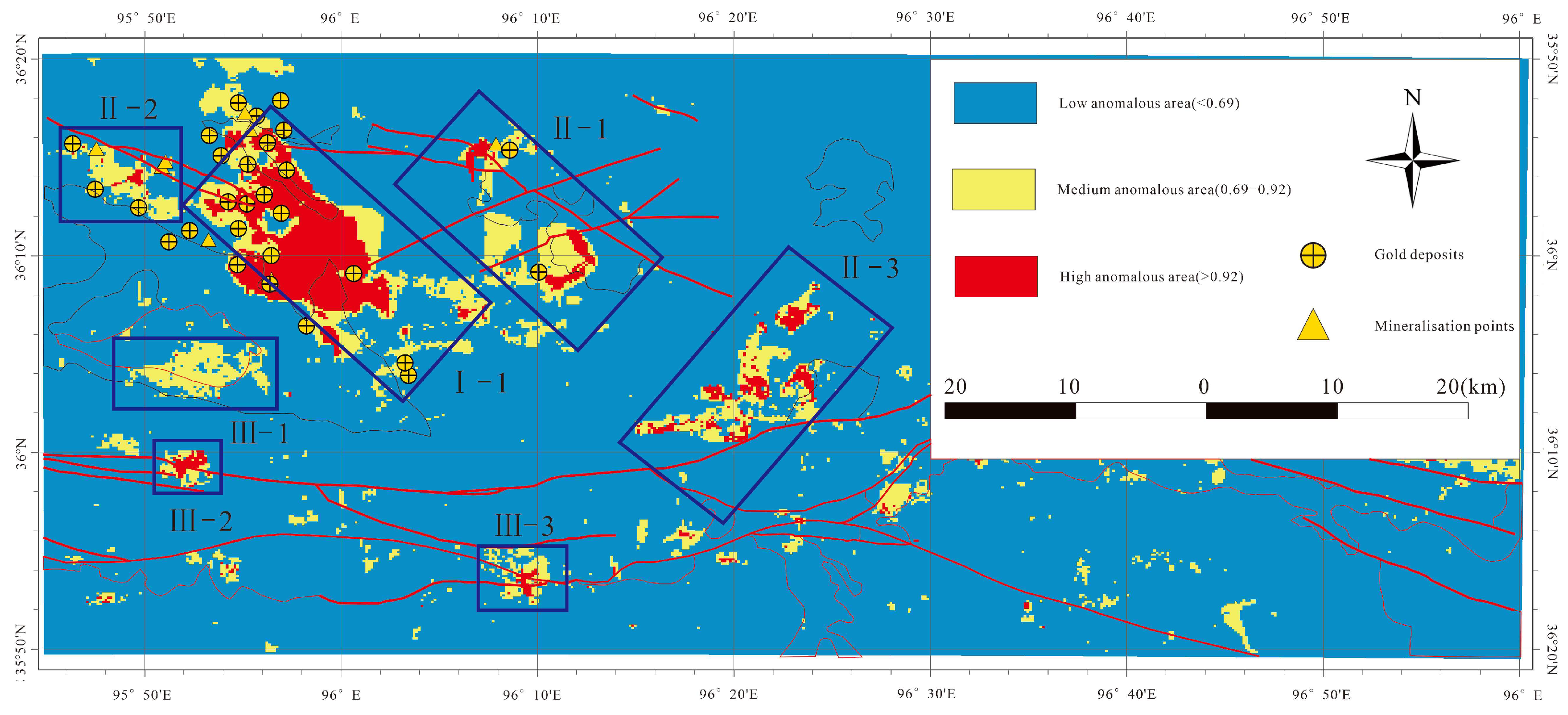
This paper identifies seven high-probability predicted targets based on the results of the BO-RF algorithm following the identification of geochemical anomalies (Figure 17).
Based on the geochemical anomaly results identified by the BO-RF algorithm, combined with the model’s predicted probability values and known mineralization information, this study adopts the following principles for the classification and delineation of prospecting targets: (1) Class I targets: areas with predicted probability values in the high-value zone (cumulative area proportion range of 96.77%–100%) that must contain known large- to medium-sized deposits and exhibit favorable metallogenic geological conditions; (2) Class II targets: areas with predicted probability values in either the high-value zone or the medium-value zone (cumulative area proportion range of 90.99%–96.77%) that contain known mineral occurrences or mineralization points and exhibit relatively favorable metallogenic geological conditions; (3) Class III targets: areas with predicted probability values in the medium-value zone (cumulative area proportion range of 90.99%–96.77%) that currently lack known mineralization but display significant geochemical anomalies or favorable metallogenic conditions, indicating further exploration potential. Based on these principles, a total of seven prospective targets of different classes were delineated within the study area (Figure 17).
Class I target (I-1) is located in the Shenshuitan-Wuminggou-Baitongou area, primarily exposing the Paleoproterozoic Jinshuikou Group gneiss formation and the contact zone with Late Silurian quartz diorite. Multiple large- and medium-sized gold deposits have been discovered in this area, some of which are associated with Cu, Pb, and Zn. The presence of two large gold deposits indicates significant metallogenic potential. All deposits in this area are classified as tectonic altered rock-type gold deposits, with gold mineralization directly occurring within the alteration zones. Except for the Wuminggou-Baitongou large gold deposit, the Hashiwa gold deposit, and the gold deposit located on the eastern side of the middle reaches of Xintuo and Wulonggou, which formed during the Caledonian period, all other deposits are of Indosinian origin. The ore bodies exhibit vein-like, lenticular, or layered structures and are relatively concentrated in distribution.
Class II targets comprise three areas. Target II-1 is situated between Dagraddong and Hope Gully, containing one mineralization point and two ore occurrences associated with Zn, Ni, Ag, and Pb. This area is mainly composed of the Neoarchean to Paleoproterozoic Jinshuikou Group Baishahe Formation, with the predominant lithology being gray-black mafic plagioclase gneiss, along with some granulite and migmatite. The mineralization points are also classified as tectonic altered rock-type gold deposits formed during the Indosinian period. Target II-2 contains one small gold deposit, two ore occurrences, and three mineralization points. Except for two hydrothermal mineralization points, all deposits in this area are tectonic altered rock-type gold deposits, also formed during the Indosinian period. Target II-3 exhibits a distinct concentration center in geochemical anomaly identification; however, no known gold mineralization points have been discovered to date. The main lithologies include medium- to fine-grained syenite granite from the Middle Triassic Dongdakender Superunit and low-grade metamorphic rocks from the Mesoproterozoic Jixian System Langyashan Formation, suggesting certain prospecting potential that requires further verification.
Class III targets include two areas. Target III-1, although relatively small in size, displays a significant distribution of high geochemical anomalies and is situated relatively close to the plate boundary, indicating further exploration potential that requires engineering verification. Target III-2 exposes clastic rocks, carbonate rocks, and mafic volcanic rocks from the upper and lower parts of the Meso-Neoproterozoic Wanbao Group, characterized by dense fault structures and notable high-probability metallogenic areas, suggesting considerable prospecting potential as well.

Author Contributions

Conceptualization, X.R.; methodology, X.R.; software, X.R.; validation, X.R.; formal analysis, X.R.; investigation, X.R.; resources, G.W.; data curation, X.R.; writing—original draft preparation, X.R.; writing—review and editing, X.R.; visualization, X.R.; supervision, G.W. and N.M.; project administration, G.W.; funding acquisition, G.W. All authors have read and agreed to the published version of the manuscript.

Funding

The authors acknowledge the funding by the National Science and Technology Major Project (Grant No. 2024ZD1001900), the Beijing Key Laboratory of Land and Resources Information Research and Development (Grant No. BJNRR2025-00), the Technology Innovation Center for Exploration and Exploitation of Strategic Mineral Resources in Plateau Desert Region, Ministry of Natural Resources (Grant No. KFKT20230102).

Data Availability Statement

Due to legal reasons, the participants in this study did not agree to publicly share their data, so supporting data is not provided.

Acknowledgments

The authors thank Ruixi Li, Xuebing Zhao, Siyan Qi, Mengxue Guo, Mingming Wang, Weitong Zhang and other group members for their help in this study. The authors thank all those who helped with this article.

Conflicts of Interest

The authors declare no conflicts of interest. The funders had no role in the design of the study; in the collection, analyses, or interpretation of data; in the writing of the manuscript; or in the decision to publish the results.

References

  1. Agterberg, F.P.; Bonham-Carter, G.F.; Wright, D.F. Statistical pattern integration for mineral exploration. In Computer Applications in Resource Estimation, Computers and Geology; Gaál, G., Merriam, D.F., Eds.; Pergamon: Amsterdam, Netherlands, 1990; pp. 1–21. [Google Scholar] [CrossRef]
  2. Maepa, F.; Smith, R.S.; Tessema, A. Support vector machine and artificial neural network modelling of orogenic gold prospectivity mapping in the swayze greenstone belt, Ontario, Canada. Ore Geol. Rev. 2021, 130, 103968. [Google Scholar] [CrossRef]
  3. Aranha, M.; Porwal, A.; González-Álvarez, I. Targeting REE deposits associated with carbonatite and alkaline complexes in northeast India. Ore Geol. Rev. 2022, 148, 105026. [Google Scholar] [CrossRef]
  4. Esmaeiloghli, S.; Tabatabaei, S.H.; Carranza, E.J.M. Spatio-geologically informed fuzzy classification: An innovative method for recognition of mineralization-related patterns by integration of elemental, 3D spatial, and geological information. Nat. Resour. Res. 2021, 30, 989–1010. [Google Scholar] [CrossRef]
  5. Mou, N.; Wang, G.; Sun, X. Identification of geochemical anomalies related to mineralization: A case study from porphyry copper deposits in the qulong-jiama mining district of Tibet, China. J. Geochem. Explor. 2023, 244, 107126. [Google Scholar] [CrossRef]
  6. Mou, N.; Carranza, E.J.M.; Xue, J.; Zhang, S.; Wang, G.; Song, H.; Chen, Y.; Ren, X. Interpretable machine learning for mineral prospectivity mapping in the Qulong–Jiama district, Tibet, China. Ore Geol. Rev. 2025, 182, 106659. [Google Scholar] [CrossRef]
  7. Zuo, R.; Wang, J.; Xiong, Y.; Wang, Z. The processing methods of geochemical exploration data: Past, present, and future. Appl. Geochem. 2021, 132, 105072. [Google Scholar] [CrossRef]
  8. Zuo, R.; Xiong, Y. Geodata science and geochemical mapping. J. Geochem. Explor. 2020, 209, 106431. [Google Scholar] [CrossRef]
  9. Zhang, S.; Xiao, K.; Carranza, E.J.M.; Yang, F.; Zhao, Z. Integration of auto-encoder network with density-based spatial clustering for geochemical anomaly detection for mineral exploration. Comput. Geosci. 2019, 130, 43–56. [Google Scholar] [CrossRef]
  10. Zhang, S.; Carranza, E.J.M.; Xiao, K.; Chen, Z.; Li, N.; Wei, H.; Xiang, J.; Sun, L.; Xu, Y. Geochemically Constrained Prospectivity Mapping Aided by Unsupervised Cluster Analysis. Nat. Resour. Res. 2021, 30, 1955–1975. [Google Scholar] [CrossRef]
  11. Bölviken, B.; Stokke, P.R.; Feder, J.; Jössang, T. The fractal nature of geochemical landscapes. J. Geochem. Explor. 1992, 43, 91–109. [Google Scholar] [CrossRef]
  12. Ghezelbash, R.; Maghsoudi, A.; Daviran, M. Combination of multifractal geostatistical interpolation and spectrum–area (S–a) fractal model for cu–au geochemical prospects in feizabad district, NE iran. Arab. J. Geosci. 2019, 12, 152. [Google Scholar] [CrossRef]
  13. Thiombane, M.; Di Bonito, M.; Albanese, S.; Zuzolo, D.; Lima, A.; De Vivo, B. Geogenic versus anthropogenic behaviour and geochemical footprint of al, na, K and P in the campania region (southern Italy) soils through compositional data analysis and enrichment factor. Geoderma 2019, 335, 12–26. [Google Scholar] [CrossRef]
  14. Kürzl, H. Exploratory data analysis: Recent advances for the interpretation of geochemical data. J. Geochem. Explor. 1988, 30, 309–322. [Google Scholar] [CrossRef]
  15. Reimann, C.; Filzmoser, P.; Garrett, R.G. Background and threshold: Critical comparison of methods of determination. Sci. Total Environ. 2005, 346, 1–16. [Google Scholar] [CrossRef]
  16. Cheng, Q.; Zhao, P. Singularity theories and methods for characterizing mineralization processes and mapping geo-anomalies for mineral deposit prediction. Geosci. Front. 2011, 2, 67–79. [Google Scholar] [CrossRef]
  17. Jin, Y.; Wu, Y.; Li, H.; Zhao, M.; Pan, J. Definition of fractal topography to essential understanding of scale-invariance. Sci. Rep. 2017, 7, 46672. [Google Scholar] [CrossRef] [PubMed]
  18. Cheng, Q.; Agterberg, F.P.; Ballantyne, S.B. The separation of geochemical anomalies from background by fractal methods. J. Geochem. Explor. 1994, 51, 109–130. [Google Scholar] [CrossRef]
  19. Cheng, Q.; Agterberg, F.P. Multifractal modeling and spatial point processes. Math. Geol. 1995, 27, 831–845. [Google Scholar] [CrossRef]
  20. Cheng, Q. Modeling local scaling properties for multiscale mapping. Vadose Zone J. 2008, 7, 525–532. [Google Scholar] [CrossRef]
  21. Cheng, Q. Singularity theory and methods for mapping geochemical anomalies caused by buried sources and for predicting undiscovered mineral deposits in covered areas. J. Geochem. Explor. 2012, 122, 55–70. [Google Scholar] [CrossRef]
  22. Chen, G.; Cheng, Q. Singularity analysis based on wavelet transform of fractal measures for identifying geochemical anomaly in mineral exploration. Comput. Geosci. 2016, 87, 56–66. [Google Scholar] [CrossRef]
  23. Wang, G.; Zhang, S.; Yan, C.; Xu, G.; Ma, M.; Li, K.; Feng, Y. Application of the multifractal singular value decomposition for delineating geophysical anomalies associated with molybdenum occurrences in the luanchuan ore field (China). J. Appl. Geophys. 2012, 86, 109–119. [Google Scholar] [CrossRef]
  24. Akbari, S.; Ramazi, H.; Ghezelbash, R. Using fractal and multifractal methods to reveal geophysical anomalies in sardouyeh district, kerman, iran. Earth Sci. Inf. 2023, 16, 2125–2142. [Google Scholar] [CrossRef]
  25. Daviran, M.; Maghsoudi, A.; Cohen, D.R.; Ghezelbash, R.; Yilmaz, H. Assessment of various fuzzy c-mean clustering validation indices for mapping mineral prospectivity: Combination of multifractal geochemical model and mineralization processes. Nat. Resour. Res. 2020, 29, 229–246. [Google Scholar] [CrossRef]
  26. Yaisamut, O.; Xie, S.; Charusiri, P.; Dong, J.; Wen, W. Prediction of au-associated minerals in eastern thailand based on stream sediment geochemical data analysis by S-a multifractal model. Minerals 2023, 13, 1297. [Google Scholar] [CrossRef]
  27. Behera, S.; Panigrahi, M.K. Gold prospectivity mapping in the Sonakhan Greenstone Belt, Central India: A knowledge-driven guide for target delineation in a region of low exploration maturity. Nat. Resour. Res. 2021, 30, 4009–4045. [Google Scholar] [CrossRef]
  28. Behera, S.; Panigrahi, M.K. Gold prospectivity mapping and exploration targeting in Hutti-Maski schist belt, India: Synergistic application of Weights-of-Evidence (WOE), Fuzzy Logic (FL) and hybrid (WOE-FL) models. J. Geochem. Explor. 2022, 235, 106963. [Google Scholar] [CrossRef]
  29. Grunsky, E.C.; de Caritat, P. State-of-the-art analysis of geochemical data for mineral exploration. Geochem.-Explor. Environ. Anal. 2020, 20, 217–232. [Google Scholar] [CrossRef]
  30. Reichstein, M.; Camps-Valls, G.; Stevens, B.; Jung, M.; Denzler, J.; Carvalhais, N.; Prabhat. Deep learning and process understanding for data-driven Earth system science. Nature 2019, 566, 195–204. [Google Scholar] [CrossRef]
  31. Shi, L.; Zuo, R. Geological Knowledge-Embedding Transfer-Learning Architecture for Geochemical Anomaly Identification. Math. Geosci. 2025, 57, 821–844. [Google Scholar] [CrossRef]
  32. Yang, Z.; Chen, Y. Anomaly Detection-Oriented Positive-Unlabeled Metric Learning for Extracting High-Dimensional Geochemical Anomalies Linked to Mineralization. Nat. Resour. Res. 2025, 34, 1219–1241. [Google Scholar] [CrossRef]
  33. Yang, F.; Wang, Z.; Zuo, R.; Sun, S.; Zhou, B. Quantification of uncertainty associated with evidence layers in mineral prospectivity mapping using direct sampling and convolutional neural network. Nat. Resour. Res. 2023, 32, 79–98. [Google Scholar] [CrossRef]
  34. Zhang, Z.; Wang, G.; Carranza, E.J.M.; Du, J.; Li, Y.; Liu, X.; Su, Y. An uncertainty-quantification machine learning framework for data-driven three-dimensional mineral prospectivity mapping. Nat. Resour. Res. 2024, 33, 1393–1411. [Google Scholar] [CrossRef]
  35. Tesoriero, A.J.; Wherry, S.A.; Dupuy, D.I.; Johnson, T.D. Predicting redox conditions in groundwater at a national scale using random forest classification. Environ. Sci. Technol. 2024, 58, 5079–5092. [Google Scholar] [CrossRef]
  36. Wang, Q.; Zhang, J.; Pan, L.; Huang, Q.; Ma, C.; Li, J.; Pan, Y. Geochronological and sulfide geochemical evidence for gold mineralization related to post-collisional magmatism in the wulonggou goldfield of the east kunlun orogen, northern tibet. Ore Geol. Rev. 2024, 170, 106155. [Google Scholar] [CrossRef]
  37. Breiman, L. Random Forests. Mach. Learn. 2001, 45, 5–32. [Google Scholar] [CrossRef]
  38. Ho, T.K. The random subspace method for constructing decision forests. IEEE Trans. Pattern Anal. Mach. Intell. 1998, 20, 832–844. [Google Scholar] [CrossRef]
  39. Köhler, M.; Hanelli, D.; Schaefer, S.; Barth, A.; Knobloch, A.; Hielscher, P.; Cardoso-Fernandes, J.; Lima, A.; Teodoro, A.C. Lithium potential mapping using artificial neural networks: A case study from central portugal. Minerals 2021, 11, 1046. [Google Scholar] [CrossRef]
  40. Lv, X.; Yang, W.; Liu, X.; Wang, G. Applications of radial basis functional link networks in the exploration for lala copper deposits in sichuan province, China. Minerals 2022, 12, 352. [Google Scholar] [CrossRef]
  41. Durdağ, D.; Ayhan Durdağ, G.; Pekşen, E. Inversion of self-potential data using generalized regression neural network. Acta Geod. Geophys. 2022, 57, 589–608. [Google Scholar] [CrossRef]
  42. Abedi, M.; Norouzi, G.-H.; Bahroudi, A. Support vector machine for multi-classification of mineral prospectivity areas. Comput. Geosci. 2012, 46, 272–283. [Google Scholar] [CrossRef]
  43. Rai, N.; Singha, D.K.; Chatterjee, R. 3D model of water saturation, effective porosity and volume of shale in upper assam shelf, India using multi-attribute regression and cascade-probabilistic neural network. J. Appl. Geophys. 2023, 218, 105202. [Google Scholar] [CrossRef]
  44. Daruna, A.; Zadorozhnyy, V.; Lukoczki, G.; Chiu, H.-P. Enabling Scalable Mineral Exploration: Self-Supervision and Explainability. In Proceedings of the 2024 IEEE International Conference on Big Data (BigData), Washington, DC, USA, 15–18 December 2024; pp. 2090–2099. [Google Scholar] [CrossRef]
  45. Chen, J.; Fu, L.; Selby, D.; Wei, J.; Zhao, X.; Zhou, H. Multiple episodes of gold mineralization in the east kunlun orogen, western central orogenic belt, China: Constraints from re-os sulfide geochronology. Ore Geol. Rev. 2020, 123, 103587. [Google Scholar] [CrossRef]
  46. Xiong, J.; Li, Y.; Li, H.; Yan, M.; Xi, J.; Wei, J. Middle triassic cu–pb–zn skarn mineralization in the wulonggou gold ore field, eastern kunlun orogen, NW China: Insights from phlogopite ar–ar and zircon U–pb dating and sr–nd–pb–hf isotopes. Ore Geol. Rev. 2024, 170, 106131. [Google Scholar] [CrossRef]
  47. Zhang, J.; Pan, L.; Wang, Q.; Huang, Q.; Ma, C.; Li, J.; Pan, Y. Generation of ore-forming magmas in transcrustal plumbing systems: Insights from the late triassic wulonggou porphyries in the eastern kunlun orogen, western China. J. Asian Earth Sci. 2023, 247, 105605. [Google Scholar] [CrossRef]
  48. Liu, Y.; Cheng, Q.; Xia, Q.; Wang, X. Application of singularity analysis for mineral potential identification using geochemical data—A case study: Nanling W–sn–mo polymetallic metallogenic belt, south China. J. Geochem. Explor. 2013, 134, 61–72. [Google Scholar] [CrossRef]
  49. Zuo, R. Identification of geochemical anomalies associated with mineralization in the fanshan district, fujian, China. J. Geochem. Explor. 2014, 139, 170–176. [Google Scholar] [CrossRef]
  50. Egozcue, J.J.; Pawlowsky-Glahn, V.; Mateu-Figueras, G.; Barceló-Vidal, C. Isometric Logratio Transformations for Compositional Data Analysis. Math. Geol. 2003, 35, 279–300. [Google Scholar] [CrossRef]
  51. Hawkes, J. Geochemistry in Mineral Exploration; Harper & Row: New York, NY, USA, 1963. [Google Scholar]
  52. Tukey, J.W. Exploratory Data Analysis; Addison-Wesley: Reading, MA, USA, 1977. [Google Scholar]
  53. Daya, A.A. Comparative study of C–a, C–P, and N–S fractal methods for separating geochemical anomalies from background: A case study of kamoshgaran region, northwest of iran. J. Geochem. Explor. 2015, 150, 52–63. [Google Scholar] [CrossRef]
  54. Arias, M.; Gumiel, P.; Sanderson, D.J.; Martin-Izard, A. A multifractal simulation model for the distribution of VMS deposits in the spanish segment of the iberian pyrite belt. Comput. Geosci. 2011, 37, 1917–1927. [Google Scholar] [CrossRef]
  55. Lowe, D.; Broomhead, D. Multivariable functional interpolation and adaptive networks. Complex Syst. 1988, 2, 321–355. [Google Scholar]
  56. Looney, C.G. Pattern Recognition Using Neural Networks: Theory and Algorithms for Engineers and Scientists; Oxford University Press: Oxford, UK, 1997. [Google Scholar]
  57. Nykänen, V. Radial basis functional link nets used as a prospectivity mapping tool for orogenic gold deposits within the central lapland greenstone belt, northern fennoscandian shield. Nat. Resour. Res. 2008, 17, 29–48. [Google Scholar] [CrossRef]
  58. Tessema, A. Mineral systems analysis and artificial neural network modeling of chromite prospectivity in the western limb of the bushveld complex, South Africa. Nat. Resour. Res. 2017, 26, 465–488. [Google Scholar] [CrossRef]
  59. Niros, A.D.; Tsekouras, G.E. A novel training algorithm for RBF neural network using a hybrid fuzzy clustering approach. Fuzzy Sets Syst. 2012, 193, 62–84. [Google Scholar] [CrossRef]
  60. Looney, C.G. Radial basis functional link nets and fuzzy reasoning. Neurocomputing 2002, 48, 489–509. [Google Scholar] [CrossRef]
  61. Sun, D.; Xu, J.; Wen, H.; Wang, D. Assessment of landslide susceptibility mapping based on bayesian hyperparameter optimization: A comparison between logistic regression and random forest. Eng. Geol. 2021, 281, 105972. [Google Scholar] [CrossRef]
  62. Aitchison, J. The statistical analysis of compositional data. J. R. Stat. Soc. Ser. B 1982, 44, 139–160. [Google Scholar] [CrossRef]
  63. Sawatzky, D.L.; Raines, G.L.; Bonham-Carter, G.F.; Looney, C.G. Spatial Data Modeller (SDM): ArcMAP 9.3 Geoprocessing Tools for Spatial Data Modelling Using Weights of Evidence, Logistic Regression, Fuzzy Logic and Neural Networks. 2009. Available online: https://codesharing.arcgis.com/?dbid=15341 (accessed on 15 May 2025).
  64. Porwal, A.; Carranza, E.J.M.; Hale, M. Artificial Neural Networks for Mineral-Potential Mapping: A Case Study from Aravalli Province, Western India. Nat. Resour. Res. 2003, 12, 155–171. [Google Scholar] [CrossRef]
Figure 1. (a) Geotectonic position of the East Kunlun Orogenic Belt; (b) Tectonic schematic map.
Minerals 16 00411 g001
Figure 2. Simplified geological map of the study area.
Minerals 16 00411 g002
Figure 3. Flow chart for illustrating the methodology.
Minerals 16 00411 g003
Figure 4. Locations of geochemical sampling map.
Minerals 16 00411 g004
Figure 5. Au Median geochemical anomaly map.
Minerals 16 00411 g005
Figure 6. Au double logarithmic diagram under S-A model.
Minerals 16 00411 g006
Figure 7. Au Background field under S-A model.
Minerals 16 00411 g007
Figure 8. Au anomalous field under S-A model.
Minerals 16 00411 g008
Figure 9. The distribution of positive and negative sample.
Minerals 16 00411 g009
Figure 10. The impact of the number of RBFs and iterations on SSE.
Minerals 16 00411 g010
Figure 11. The receiver operating characteristic curve of the optimal model of the RBFLN model.
Minerals 16 00411 g011
Figure 12. Percentage of cumulative area based on relative probability values in the RBFLN model.
Minerals 16 00411 g012
Figure 13. Geochemical anomaly map classified by the RBFLN model.
Minerals 16 00411 g013
Figure 14. The receiver operating characteristic curve of the optimal model of the BO-RF model.
Minerals 16 00411 g014
Figure 15. Percentage of cumulative area based on relative probability values in the BO-RF model.
Minerals 16 00411 g015
Figure 16. Geochemical anomaly map classified by the BO-RF model.
Minerals 16 00411 g016
Figure 17. Prospecting prediction targets and engineering verification map of the study area.
Minerals 16 00411 g017
Table 1. Descriptive statistics and enrichment coefficients of geochemical elements.
ElementAverage ValueStandard DeviationSkewnessKurtosisCoefficientEnrichment Coefficient
Au1.821241.431948.726.581.3
Ag0.070.038.25118.090.410.05
Sn2.981.375.2657.190.461.19
As10.516.626.99175.260.631.05
Sb0.930.768.77108.90.811.17
Bi0.350.3673.417745.781.021.16
Hg28.7514.216.36123.130.490.72
Pb23.919.335.1239.930.391.04
Zn64.5825.5814.53613.610.40.95
V66.9824.563.1318.280.370.82
W2.111.095.7569.660.511.17
Mo1.190.6412.16353.030.531.49
Cd0.130.031.032.390.261.45
Cr47.9542.349.43151.060.880.74
Ni24.4812.522.7511.380.510.94
Co17.256.765.9777.350.391.33
Fe2.80.870.983.240.31-
Au and Hg are 10−9; Fe is 10−2; All other elements are 10−6.
Table 2. Comparison of results from different methods.
MethodElementProbability of Ore Occurrence in Anomaly Area (n)/%Proportion of Anomalous Area (s)/%n/sAUC
MADAu41.6718.22.29-
S-AAu27.784.75.91-
BO-RF-758.938.400.84
RBFLN-5819.243.010.81
median + 2MAD is abbreviated as MAD.
Disclaimer/Publisher’s Note: The statements, opinions and data contained in all publications are solely those of the individual author(s) and contributor(s) and not of MDPI and/or the editor(s). MDPI and/or the editor(s) disclaim responsibility for any injury to people or property resulting from any ideas, methods, instructions or products referred to in the content.