Article

Magnetite Texture and Geochemistry in the Takab Ore Deposit (NW Iran): Implications for a Complex Hydrothermal Evolution

1
Sorbonne Université, CNRS-INSU, Institut des Sciences de la Terre de Paris, ISTeP, F-75005 Paris, France
2
Sorbonne Université, CNRS-INSU, Institut de Physique du Globe de Paris, IPGP, F-75005 Paris, France
3
Laboratoire Géosciences Paris-Saclay, GEOPS, Université Paris-Saclay, CNRS, F-91405 Orsay, France
4
Department of Geology, Faculty of Science, University of Zanjan, University Blvd., Zanjan 45371-38791, Iran
5
Department of Earth Sciences, Institute for Advanced Studies in Basic Sciences (IASBS), Zanjan 45137-66731, Iran
*
Author to whom correspondence should be addressed.
Minerals 2025, 15(2), 137; https://doi.org/10.3390/min15020137
Submission received: 24 September 2024 / Revised: 24 January 2025 / Accepted: 25 January 2025 / Published: 29 January 2025
(This article belongs to the Special Issue Geochemistry and Genesis of Hydrothermal Ore Deposits)

Abstract

:
The massive magnetite deposit from Takab (NW Iran) is hosted in amphibolite layers intercalated with the chemical and terrigenous sediments of the Takab BIF. A comprehensive textural and chemical study allowed three types of magnetite (Mt) to be distinguished. Mt1 forms large (≤1 mm) inhomogeneous grains surrounded and locally invaded by magnetite Mt2. Oscillatory zoning is present in Mt1 and Mt2. Mt3 forms bands aligned along fracture planes. Mt3 may contain hematite relicts and is porous in proximity to hematite. Mt1 shows variable and higher Si (up to 1.4 wt. %), Al, Ca, and Mg and lower Fe content (68 wt. %) than Mt2. Mt3 has the lowest Si (<0.3 wt. %) and highest Fe (71 wt. %) contents. The temperature of formation decreases from Mt1 (600 °C) to Mt2 (500–550 °C) and Mt3 (380–440 °C). Mt1 likely formed in a reducing Si-rich environment. The close spatial relationship, sharp compositional boundaries, similar crystallographic structure of Mt1 and Mt2, and porosity in Mt2 suggest a fluid-assisted coupled dissolution of Mt1 and precipitation of Mt2 (CDR process). Microfracturing allowed the penetration of oxidizing fluid and the formation of platy hematite bands. Mt3 (mushketovite) formed after hematite by interaction with a reducing lower temperature fluid through a redox transformation.

1. Introduction

Magnetite, a common mineral in many ore deposits, can contain minor and trace elements which have been widely used to constrain the environment of formation [1,2,3]. However, both the texture and trace-element composition of magnetite can be significantly modified or re-equilibrated by metasomatic fluids, e.g., [4,5,6,7]. Therefore, detailed studies of texture and chemical composition must be carried out to defining the processes of magnetite formation.
Iran is the ninth most important iron ore producer in the world with about 4 billion tons of iron ore annually produced from more than 200 iron deposits [8,9,10,11]. Iron ore deposits were formed during several metallogenic stages: (1) Neoproterozoic–early Cambrian, (2) late Paleozoic–early Mesozoic, and (3) Cenozoic. The largest iron ore deposits formed during stage 1, mainly as Kiruna-type (IOA, iron oxide apatite) deposits, and during stage 3, mainly as Fe-skarn deposits [12,13,14,15]. Their spatial distribution is related to the main suture zones of the fragmented Iranian continental blocks resulting from the complex evolution of the Tethyan oceans [10,16,17]. The most important iron deposits are in the Central Iranian Zone (CIZ), in the Sanandaj–Sirjan zone (SSZ), and in the Alborz (AMB)–Azerbaijan belts (Figure 1; e.g., [18,19,20] and references therein). The SSZ extends 1500 km from northwest to southeast parallel to the Zagros belt, on the east side of the Main Zagros Fault. It hosts numerous iron and iron–manganese deposits of various origins (Figure 1; [10,21]). For example, in the south of the SSZ, the major Gol-e-Gohar iron deposit and the Heneshk iron–manganese deposit are related to the opening of the Neo-Tethys Ocean and are interpreted to be of volcano–sedimentary or mixed hydrothermal and volcano–sedimentary origin [18]. Further north, the Fe-skarn-type Hamekasi iron deposits (e.g., Baba Ali) are related to the subduction and closure of the Neo-Tethys Ocean (Figure 1; [10] and references therein). In northwestern Iran, the major deposit of the Zanjan-Soltaniyeh area, which belongs to the near structural Central Iranian Zone, comprises both skarn-type and volcano–sedimentary iron deposits [10,20]. A hundred km west of Zanjan in the northwestern part of the SSZ, several iron mineralizations have been reported in the Takab area. In this area, some outcrops were initially explored in the 1990s and studied for their geology and geochemistry by a few authors: at 60 km east of Takab town (Figure 1), the Shahrak mining complex represents reserves of a total of 60 million tons of iron ore with an average Fe grade of 50% [22,23]. It comprises 10 ore deposits, among them the Korkora skarn deposit [23] and the Kosaj volcano–sedimentary-type iron deposit [24]. The iron deposit of Mianaj, near Halab (Figure 2), was also reported as a metamorphosed and folded volcano-sedimentary-type iron deposit [25]. Different petrogenetic models have been proposed, such as the superior-type BIF [26] and Algoma-type BIF [27], for the Halab and Ouzijan iron mineralizations.
In a recent study on the Takab magnetite mineralizations near Halab, Honarmand et al. [8] investigated the banded, nodular, and disseminated magnetite layers in the folded succession of micaschist and quartzite (the studied outcrops are represented by yellow circles in Figure 2). Based on geochemical, Nd isotopic, and geochronological data, they proposed that this iron ore corresponds to a Rapitan-type banded iron formation. These data indicate that it originated in a back-arc basin through iron precipitation and the incorporation of ca. 20% of the terrigenous materials in the chemical precipitates. The Neoproterozoic felsic–intermediate crystalline basement was the main sediment source [8]. Furthermore, trace-element and Fe and O isotopic investigations of the banded, nodular, and disseminated magnetite [28] support their genesis from a mixture of seawater and hydrothermal fluid environments. Isotopic data point out the complex hydrothermal history from seafloor high-T° fluid to later re-equilibration with lower-T° fluid produced during the decarbonatization of the intercalated carbonate-rich schists.
Close to the nodular and disseminated magnetite mineralization, massive magnetite layers are intercalated in amphibolite. These layers were never studied in detail for petrography, iron oxide chemistry, or textural features.
This study presents for the first time major- and trace-element electron microprobe data and EBSD analyses of the massive magnetite layers in the vicinity of banded, nodular, and disseminated magnetite layers that were previously studied.

2. Materials and Methods

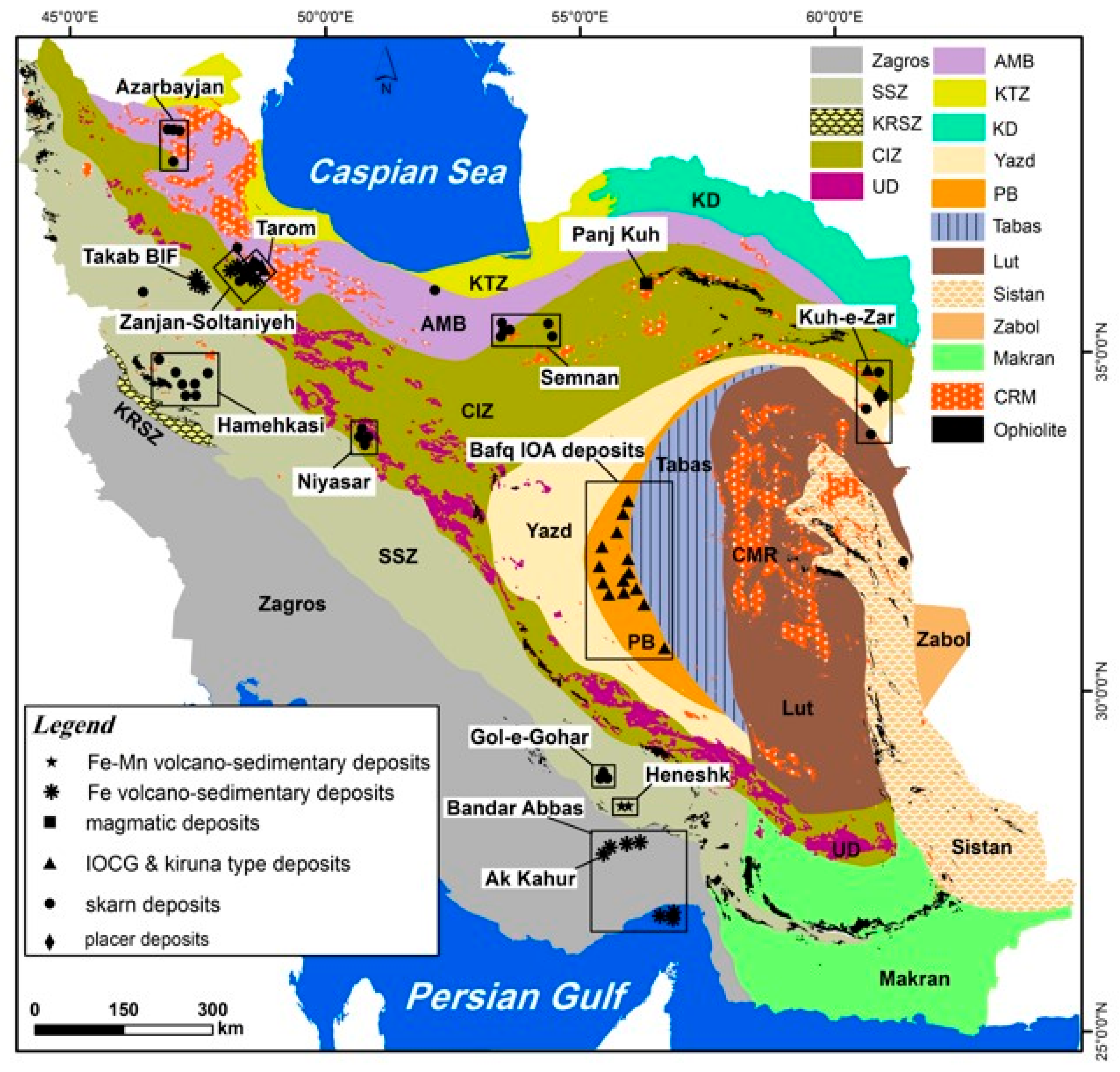
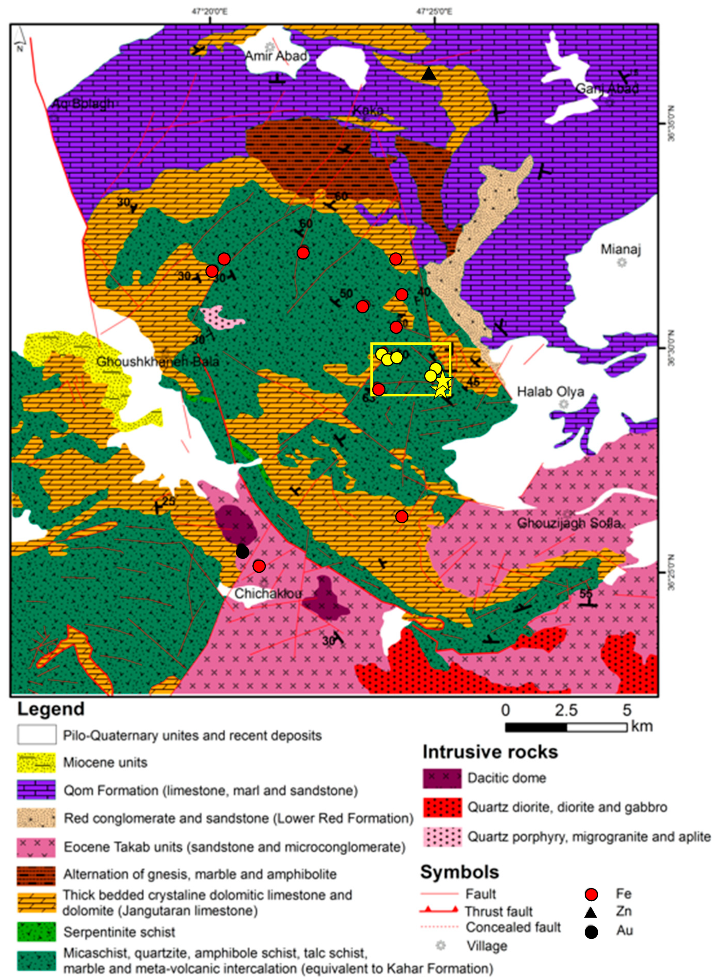
2.1. Geological Settings

The Takab area is located in the northwestern part of the Sanandaj–Sirjan magmatic-metamorphic structural zone (Figure 1). The Takab area consists of metamorphic rocks including gneisses, amphibolites, mica- and calc-schists, quartzite, jaspilite, marble, and rare granulite. These rocks were intruded by granitoids, diorite, gabbros, and rare rhyolite [8,29,30]. The area experienced several metamorphic and deformation events during the Precambrian and the Tertiary. The latter event is related to the Alpine orogeny, leading to the faulting and folding of the Precambrian metamorphic units. The Tertiary metamorphic event produced the migmatites, at ca. 25 Ma [31], and the granitoids [10,29,31].
The metamorphic units of the late Neoproterozoic–early Cambrian (548–568 Ma) age [29,31] were overlain unconformably by Tertiary sedimentary units. The lack of Paleozoic and Mesozoic rocks indicates that this region was exhumated at that time [32]. Exhumation started during the Early to Middle Jurassic back-arc extension and Tertiary crustal extension related to compressional tectonics [29]. The different rock units experienced upper greenschist to amphibolite facies metamorphism (450° to 700 °C and 0.6–1 GPa) in the Middle Jurassic. After exhumation and weathering, the ore was covered by Quaternary sediments [18].

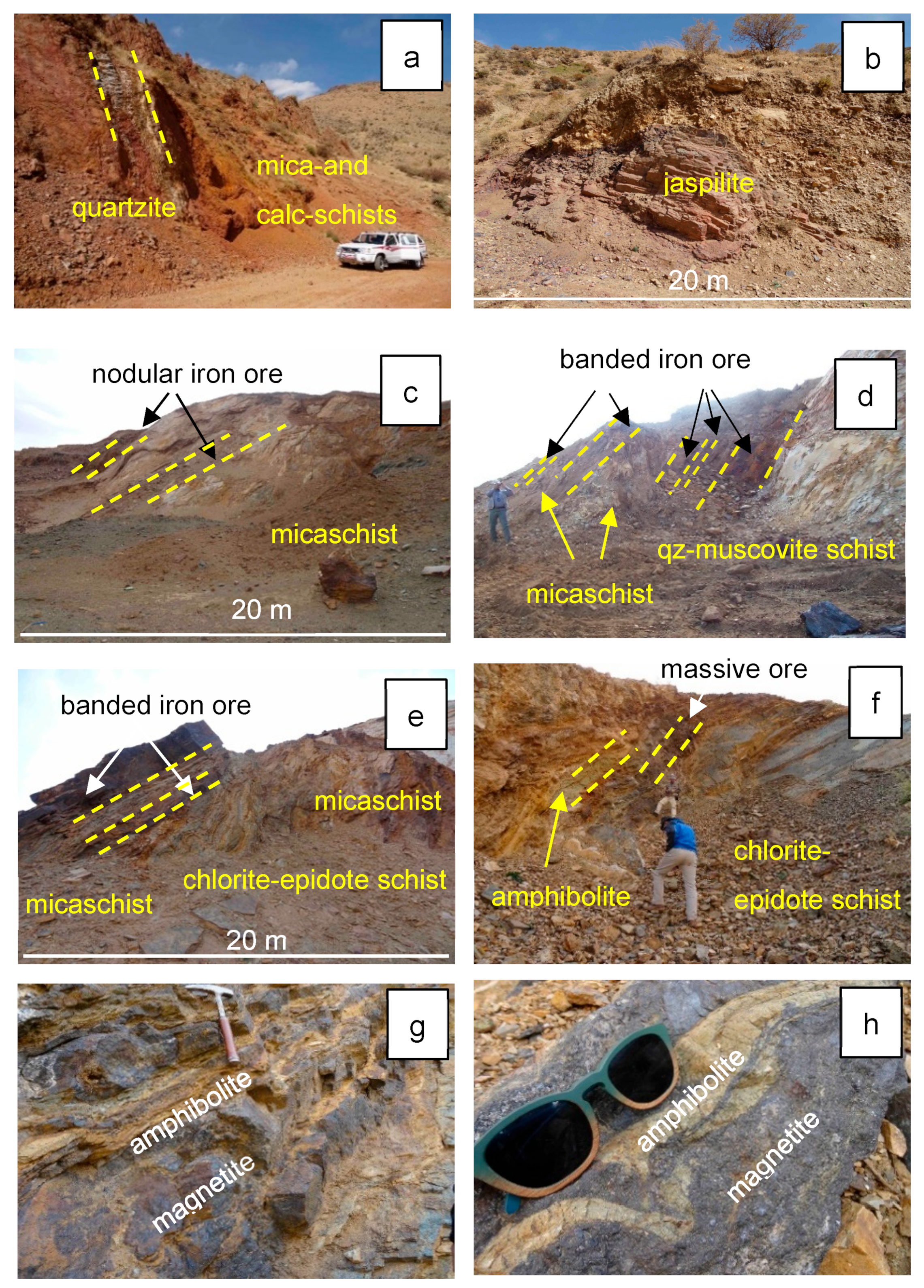
2.2. Ore Deposit and Sample Material

The Takab iron ore outcrops are located west of the village of Halab (marked area in Figure 2). Recently, Honarmand et al. [8] and Wagner et al. [28] studied outcrops of banded and nodular magnetite layers up to 2 m in thickness in the folded succession of micaschist and quartzite from the Takab BIF, 3 to 6 km west of Halab (47°23′51″ E to 47°25′39″ E longitude and 36°29′13″ N to 36°30′03″ N latitude, Figure 2, yellow circles). In this study, we investigate the massive magnetite layers intercalated with micaschist and amphibolite (former meta-basalt) in the Takab BIF. The samples were collected ca. 3 km west of Halab along an exposure 200 m in length situated at 47°25′28.1″ E and 36°29′25.5″ N (Figure 2, yellow stars).
The iron ore is hosted in a metamorphosed volcano–sedimentary sequence composed of mica- and calc-schists, quartzite, and jaspilite. Some marble and amphibolite (meta-basalt) bands are intercalated with the micaschists (Figure 3). U-Pb dating on zircons from micaschist lower and upper layers of the ore body indicates a depositional age of ca. 560 Ma [8]. The banded, nodular, and disseminated iron ore consist of magnetite, which may be partially hematized and surrounded by goethite in some samples [8,28]. The massive magnetite layers are hosted in amphibolite interlayered with the micaschists and quartz sequence. The host amphibolite is a massive, dark green rock with schistose texture (Figure 4a and Figure 5). At the microscale, transparent patches of albite (Ab92, Supplementary Table S1) and microquartz occur in a light to dark green matrix mainly composed of amphibole and minor biotite (Figure 4a). The amphibole forms elongate crystals of actinolite and a few acicular crystals of Mg-hornblende (Table 1). Actinolite hosts relicts of a more Mg-rich amphibole (Figure 4b and Table 1). Euhedral crystals of titanite, interstitial calcite, and large patches of epidote and chlorite are also present (Figure 4b–e). Chlorite is mostly developed along amphibole and mica cleavages (Figure 4d) or as a few rosette-shaped interstitial crystals. Accessories are barite (Figure 4f), rare Cl-free apatite and allanite, and late pyrite. (Figure 4g,h).
The amphibolite hosts massive magnetite layers of several tens to about one meter in thickness, which are slightly folded and/or boudinized (Figure 3g,h). The contact between the magnetite layers and the amphibolite is either abrupt or gradual (Figure 5b,c). In the magnetite layers, albite, amphibole, and minor biotite are interstitial to the magnetite crystals (Figure 5) and have the same composition as in the amphibolite (Table 1). Amphibole and mica can be locally altered to epidote, calcite, and chlorite. Rare interstitial calcite and rosette-like chlorite crystals are also observed (Figure 5f).

2.3. Analytical Methods

Three representative samples of the massive iron ore were studied. The samples were prepared as standard polished thin sections for study by optical microscopy, high-resolution scanning electron microscopy (HR-SEM), electron backscatter diffraction (EBSD), and electron microprobe analysis (EMPA).

2.3.1. Electron Microprobe Analysis

EMPA was performed with a Cameca SX100 electron microprobe equipped with five wavelength dispersive spectrometers at CAMPARIS, Sorbonne-Université, Paris, France. Fe and O were analyzed under the following operating conditions: monochromators LLIF for the measure of Fe and LPC1 for oxygen; accelerating voltage 15 kV; beam current 10 nA; counting times, 10 s over the peak and 10 s for background measured on each side of the peak; Fe2O3 as standard. WDS multi-element X-ray mapping was obtained from the same EMP.
For trace elements, monochromators were LTAP (Si, Al, and Mg) and PET (for Ca). To decrease the detection limits Ti, V, Mn, Ni, Cr, and Cu were simultaneously analyzed with LIF and LLIF monochromators on three different spectrometers. The operating conditions were 25 keV, 300 nA, 40 s to 70 s, and a beam size of 1 µm. Any damage effects on the samples were checked during analyses. The concentration of V using the Kα lines was not affected by the adjacent Ti Kβ line at the observed low Ti concentration. Standards were synthetic metal oxides and natural minerals: Ti, Mn: MnTiO3; Fe, O: Fe2O3; Al; orthoclase; Cr: Cr2O3; Ni: NiO; Mg, Si, Ca: diopside; V: vanadinite; Cu: Cu native. Carbon coating was performed simultaneously for standards and samples to ensure the same coating thickness. These settings yielded minimum detection limits, with average concentrations as low as ~3–5 for Ca, Ti, and Mn and ~11–19 ppm for Mg, Al, and Si. The concentrations in V, Ni, Cr, and Cu were below or near the detection limit (~8–15 ppm) and could not be accurately determined.

2.3.2. Scanning Electron Microscopy and Electron Backscattered Diffraction Analysis

Backscattered imaging by scanning electron microscopy (SEM) and electron backscattered diffraction (EBSD) were carried out on a ZEISS Supra 55 VP at ISTeP (Sorbonne Université, Paris, France). The EBSD analysis was performed using an ARGUSTM FSE/BSE imaging system mounted on a Bruker e-FlashFS detector. The data were processed with the ESPRIT 2.2 software package from the QUANTAX EDS/EBSD system from the Bruker Company. EBSD is detailed hereafter. Carefully polished thin sections from three samples were prepared and then analyzed uncoated by SEM. Representative areas were selected. The initial conditions were as follows: angular deviation lower than 5°, minimum pixel size of 5, and spike correction of zero-solution measurements relative to the surrounding points. EBSD measurements were used to acquire mineral phases, crystal orientations, and microstructural information. Crystal orientations are described using the set of Euler angles, and each orientation is represented by a combination of RGB colors in an Euler map. Pole figure (PF) and inverse pole figure (IPF) are also used in this study. The produced pole figures are displayed in terms of points or in contoured versions indicating the strength of the clustering of poles relative to that of a random distribution. The IPF maps were generated for the three selected viewing directions parallel to the X, Y, and Z axes, quoted as IPFX, IPFY, and IPFZ.

3. Results

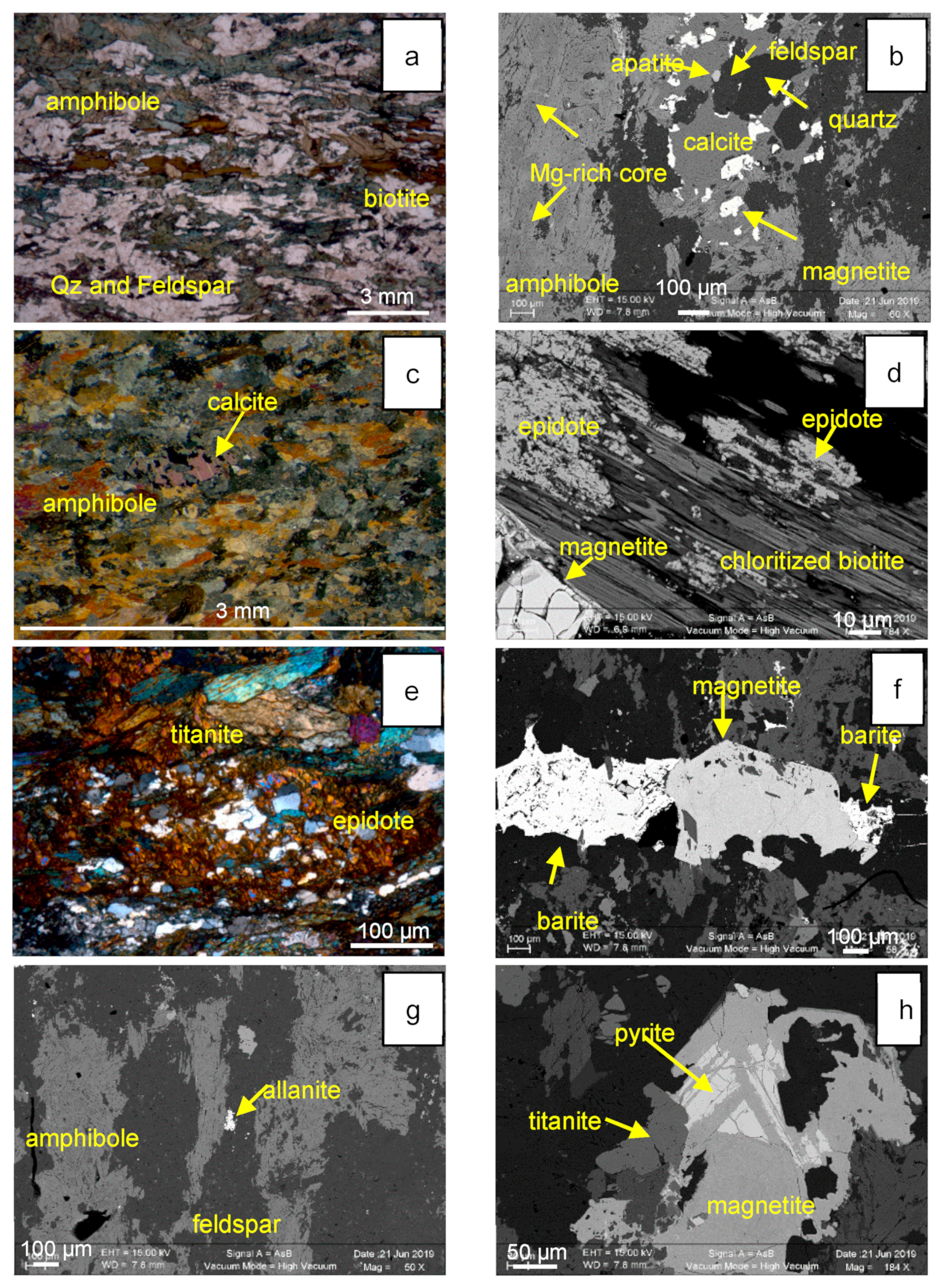
3.1. Morphology and Textures of Magnetite

Magnetite grains are enclosed in a matrix mainly composed of actinolite and albite (Figure 4). Based on BSE imaging and WDS X-ray mappings, three types of magnetite have been identified (Figure 6, Figure 7 and Figure 8).The first type (Mt1) occurs as sub- to anhedral grains of an inhomogeneous dark gray magnetite in BSE images, ranging up to 1 mm in dimension. Mt1 is surrounded by a light gray type 2 magnetite (Mt2). The boundary between Mt1 and Mt2 is usually sharp (Figure 6a, bottom right, Figure 7a) but may also locally invade dark Mt1, forming lighter gray patches (Figure 6a, upper left). Three different subtypes of Mt2 have been locally recognized in sample TAK-Z1: Mt2-A and Mt2-C are light gray on BSE images, while Mt2-B is darker gray (Figure 8). Both Mt1 and Mt2-B show an oscillatory growth zoning of dark and light zones, suggesting a higher concentration of elements with a low atomic number in the dark zones (Figure 8). Mt3 appears as bands (10–80 µm width) with needle-like textures of bright magnetite aligned along microfracture planes that crosscut the Mt1–Mt2 grains (Figure 6a and Figure 7; Supplementary Figure S1). Mt3 bands replace platy hematite, which remains as rare relict-aligned patches (Figure 6). In some bands, Mt3 appears to be porous only close to the hematite relicts. Aggregates of euhedral magnetite grains (100–200 µm) from sample TAK-Z4 also display well-developed chemical oscillatory zoning (Figure 9).

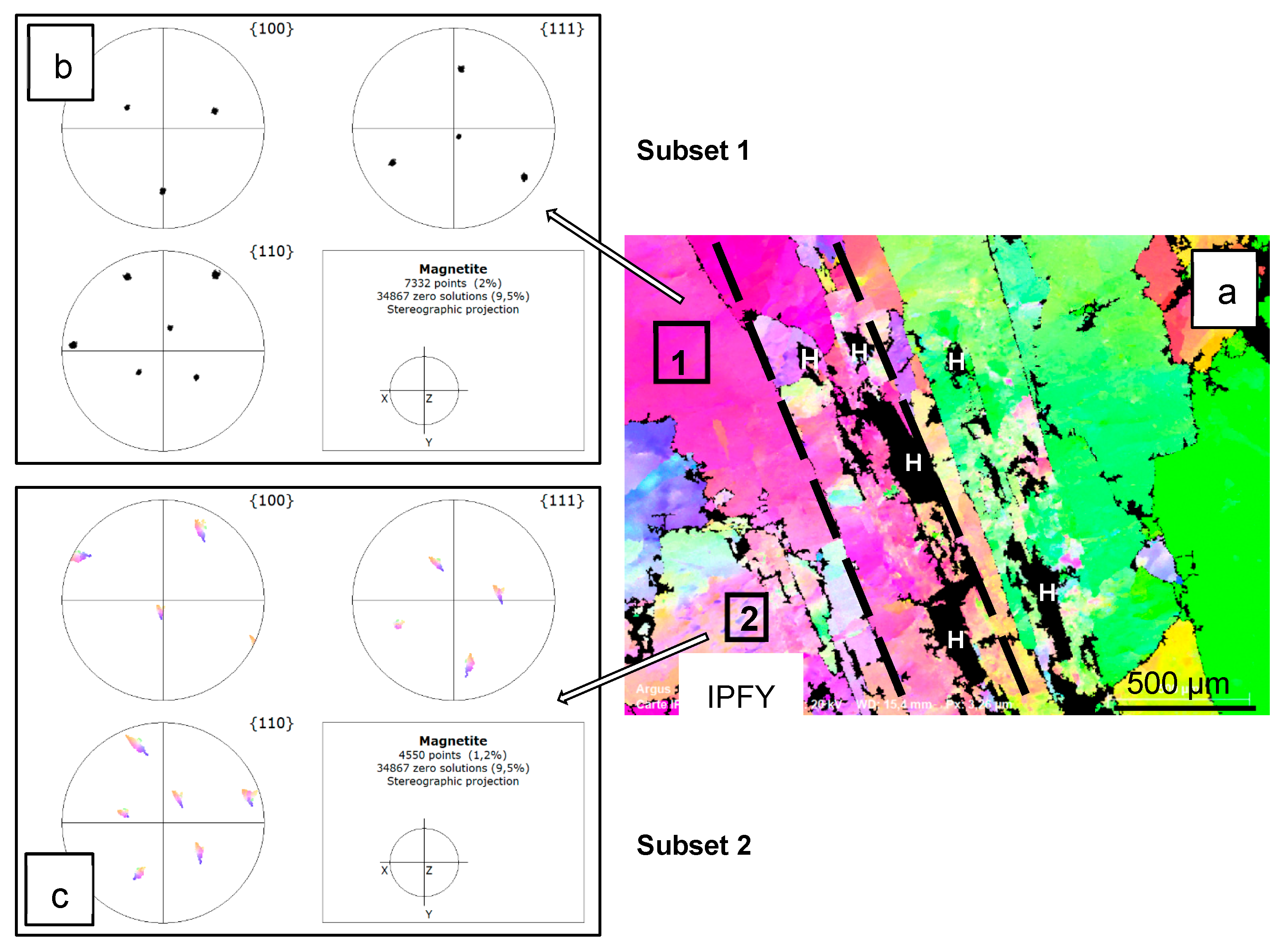
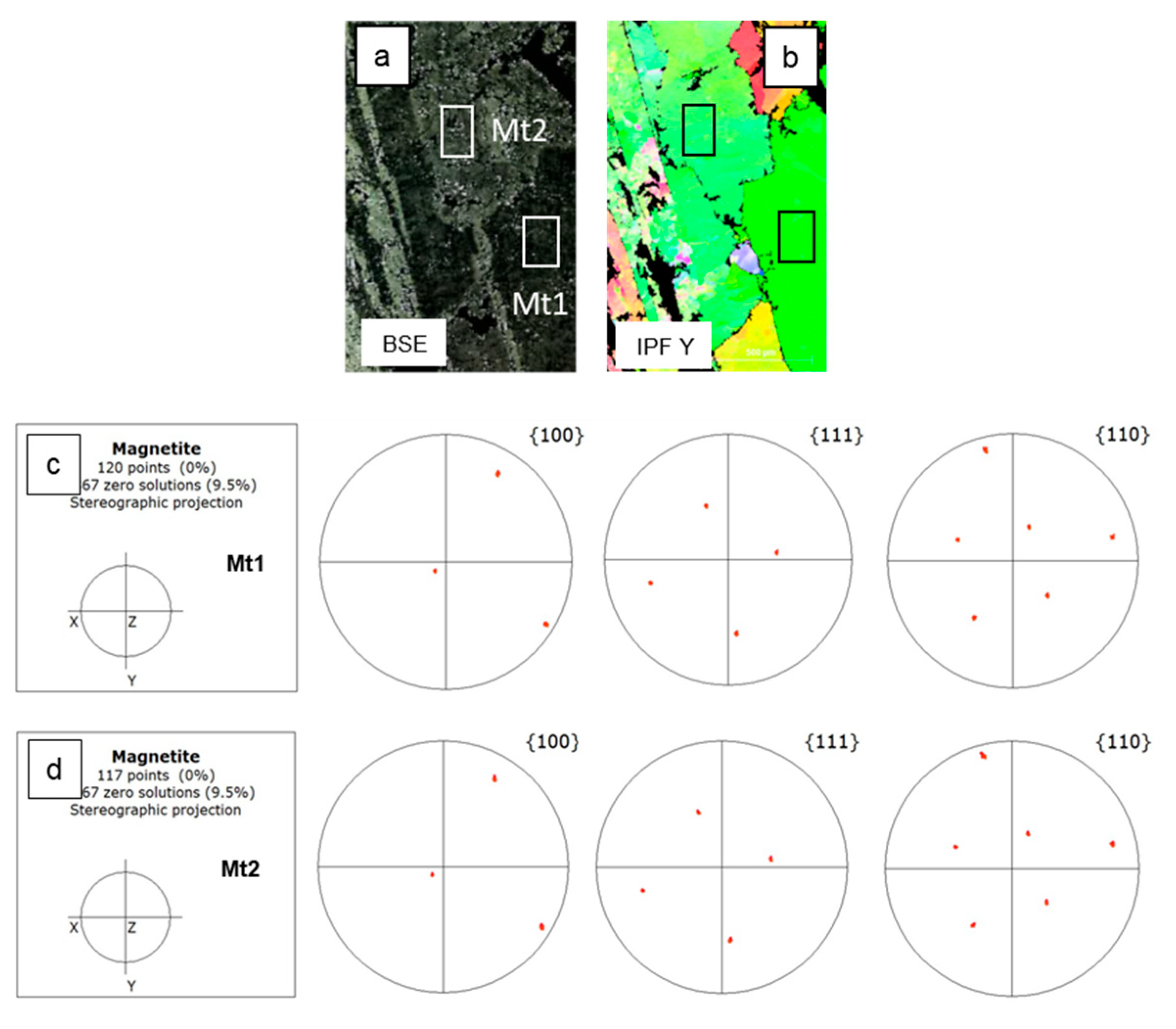
3.2. Electron Backscatter Diffraction Mapping

EBSD misorientation maps of magnetite show both sudden orientation changes across grain boundaries and gradual or wavy misorientation unrelated to grain boundaries. For example, Figure 10 shows wavy misorientation in Mt1 (lower left) as well as in the Mt3 band, delimited by the dotted lines.
A small area of the different magnetite grains was selected to generate pole figures (PFs) and inverse pole figures (IPFs). Magnetite grains with a uniform color in IPF maps show discrete point clusters in PFs, reflecting uniform intragrain orientation (Figure 10, subset 1). Magnetite grains with wavy colors show less-clustered points in PFs, and the crystal orientations may disperse along small circle girdles in stereoplots of <100>, <110>, and <110> directions in individual magnetite grains (Figure 10, subset 2), which is related to the wavy intragrain misorientation. This indicates that the intragrain microstructures formed through deformation by dislocation movement without recovery or rearrangement in subgrains [33]. Magnetite thus shows at the microscale the effect of deformation, which is observed at the macroscale by the folded magnetite layers in the host amphibolite (Figure 3g,h).

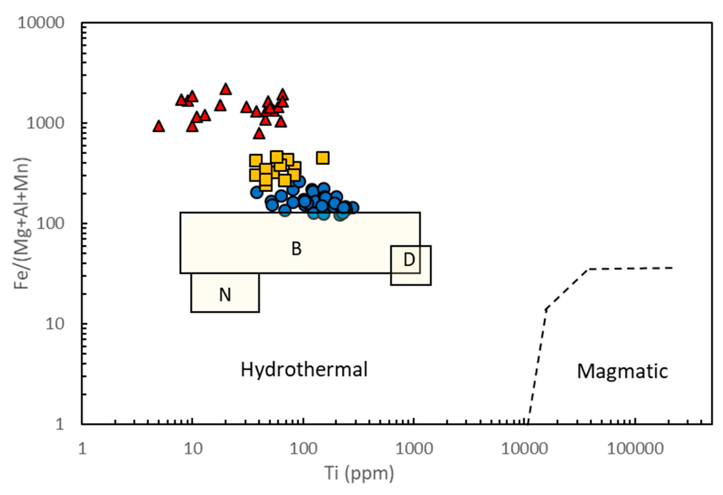
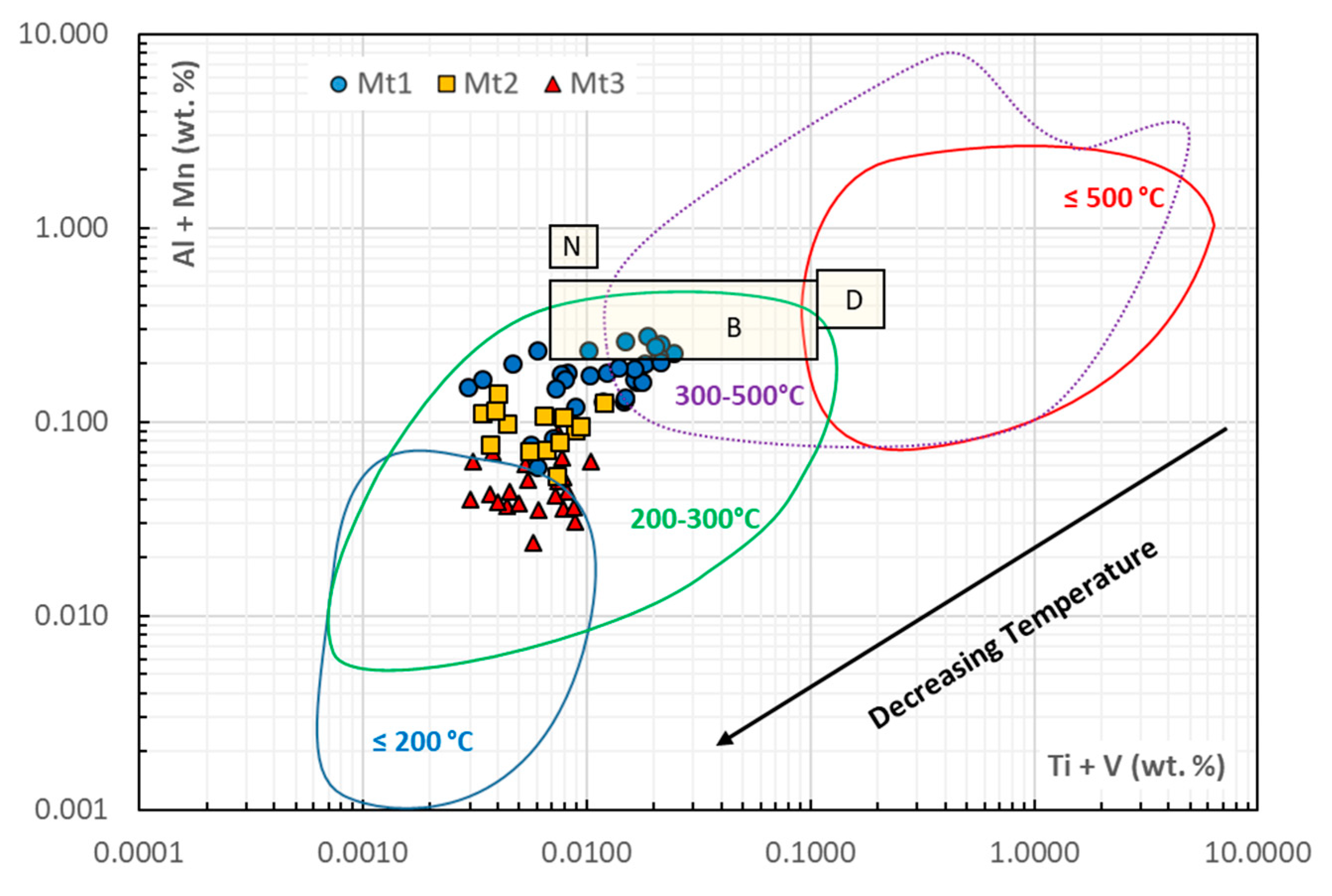
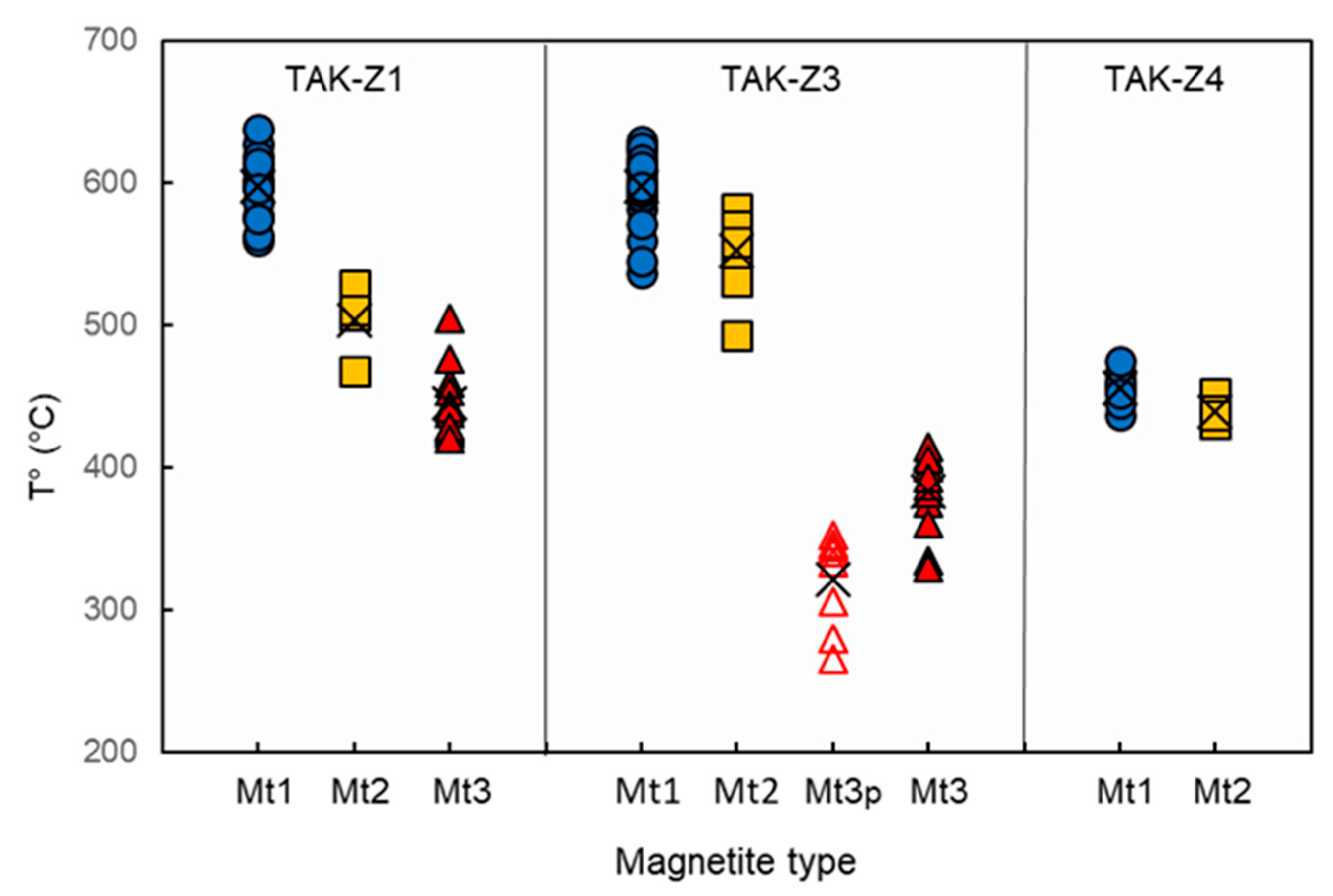
3.3. Chemical Composition of Magnetite

WDS X-ray elemental mapping was performed to determine the distribution of minor and trace elements. Si, Al, Mg, and Ca maps clearly distinguish the different magnetite types (Figure 6, Figure 7 and Figure 8; Supplementary Figure S1). Mn has a uniform distribution throughout the different magnetite types, whereas Ni, Cr, and Cu are below or close to the detection limits and thus give no information. Therefore, these elements are not further discussed here. Of the three texturally identified magnetite types, Mt1 is rich in Si, Al, Mg, and Ca (Figure 6, Figure 7 and Figure 8). Mt2 shows variable enrichment or depletion of Si, Al, Mg, and Ca in the different zones Mt2-A, -B, and -C (Figure 8). Magnetite from zone Mt2-B presents oscillatory enrichment or depletion, which is also observed in magnetite Mt1 (Figure 8) and magnetite from the aggregates (Figure 9). Mt3 is characterized by the lowest contents of these elements and by the highest Fe content (Figure 7).
The average concentrations, standard deviations, and ranges of values are listed in Table 2. The complete analytical results are given in Supplementary Table S2.
The magnetite composition is presented in Figure 11 for sample TAK-Z3, as it is representative of magnetite from the three studied samples. In the three samples of magnetite, Mt1 has the most variable composition and the lowest Fe content (66–68 wt. %), while both Mt2 and Mt3 show a restricted range of composition in minor and trace elements (Figure 11a, b) and higher Fe contents (70 and 71 wt. %, respectively). In the three samples, Mt1 magnetite has high contents of Si (0.83–1.38 wt. %) and moderately high Al (0.14–0.35 wt. %), Ca (0.16–0.38 wt. %), and Mg (0.06–0.19 wt. %). Mt2 magnetite has lower Si (0.32–0.72 wt. %), Ca (0.10–0.22 wt. %), Al (0.08–0.16 wt. %), and Mg (0.02–0.11 wt. %). Mt3 (porous and non-porous) magnetite has the lowest minor- and trace-element contents, with Si (≪0.01–0.08 wt. %), Al (0.02–0.05 wt. %), Ca (0.02–0.08 wt. %), and Mg (≪0.01 wt. %). The three types of magnetite contain similar low Mn (0.02–0.05 wt. %), while Ti is ≪0.01 wt. % in Mt2 and Mt3 but can reach 0.04 wt. % in Mt1. Mt1 and Mt2 have low similar V contents (19–24 ppm), while Mt3 is slightly richer in V (27–34) ppm. The composition of the thin oscillatory dark and lighter gray bands in Mt1 and Mt2-B magnetite grains could not be resolved with the microprobe.

4. Discussion

4.1. Magnetite Formation Conditions

The minor- and trace-element composition of magnetite has been used in numerous studies to fingerprint its environment of formation based on a series of discrimination diagrams, e.g., [1,3,34]. However, coexisting phases may affect the composition of magnetite, for example, the co-precipitation of amphibole and epidote could decrease the incorporation of Mg and Al, respectively, in magnetite. In this study, as the different magnetite types Mt1, Mt2, and Mt3 co-crystallized with the same coexisting assemblage, any major control of the co-precipitated phases on compositional differences between the three magnetite types is unlikely.
The contents of Mg, Mn, Ti, V, Ni, and Cr in magnetite, for example, can be used to discriminate between formation in a hydrothermal or a magmatic environment. In this study, the different types of magnetite plot in the field of hydrothermal magnetite characterized by low Ti content on a Fe/(Mg + Al + Mn) discrimination diagram (Figure 12). On the V vs. Ti diagram, most of the different types of magnetite plot outside the hydrothermal field due to a very low V content (Supplementary Figure S2), which does not give here any reliable information. On the other hand, the extremely low Ni and Cr contents of all three types of magnetite (Table 2) further support a hydrothermal origin. This agrees with a previous study of the layered, nodular, and disseminated magnetite from the Takab BIF, in which it was shown that both the trace-element and Fe and O isotopic compositions provided evidence for a complex hydrothermal history [8,28].
Element partition coefficients are temperature-dependent and can therefore be used for constraining the temperature of formation of magnetite. The incorporation of Ti increases with temperature in magmatic and in high-temperature hydrothermal environments, whereas it is negligible in low-temperature hydrothermal fluids [35,36]. Discriminating diagrams, such as (Al + Mn)/(Ti + V), have been proposed to outline different fields of temperature [3,37]. As can be seen in Table 2 and Figure 11, magnetite Mt1 has a variable composition with up to 1.4 wt. % Si and up to 0.4 wt. % Al. This raises the question of whether Si is really incorporated in the magnetite structure or present as Si-bearing nanoparticles [37,38,39]. In the absence of a definitive argument (as discussed below in Section 4.1), we tentatively estimated the possible contamination of the analyses of magnetite by nanoinclusions of amphibole at 5–6% (Supplementary Figure S3). The appropriate correction was applied before using the (Al + Mn)/(Ti + V) diagram and temperature calculations.
The decreasing trend shown in the (Al + Mn)/(Ti + V) diagram (Figure 13) indicates a decreasing temperature from Mt1 to M2 and Mt3. Overall, the different magnetite types formed at medium temperature ca. 300 °C or 200–300 °C. These temperature ranges are similar although slightly lower than that those recorded by the banded, nodular, and disseminated magnetite previously studied [28], shown by the rectangles in Figure 13.
Canil and Lacourse [40] proposed a T°Mg-mag empirical geothermometer, T°Mg-mag = −8344 (±320)/[lnXMg − 4.1 (±0.28)] − 273, that was applied to magnetite from various settings: igneous rocks, hydrothermally altered rocks, and ore deposits. Figure 14 presents the results of the T°Mg-mag calculations of the three magnetite types excluding the analytical points from the areas showing oscillatory zoning in magnetite Mt1 and Mt2b. The data are presented in Supplementary Table S3.
A decreasing trend is evidenced from magnetite Mt1 to Mt2 and Mt3 in samples TAK-Z1 and TAK-Z3, whereas in sample TAK-Z4, magnetite Mt1 and Mt2 from the agglomerates formed at a similar temperature. In sample TAK-Z3, the porous magnetite Mt3 records lower temperature than the non-porous magnetite Mt3. However, the calculated temperatures are much higher than those estimated from the (Al + Mn)/(Ti + V) diagram (Figure 13): e.g., average 600 °C for Mt1, 500 °C for Mt2, and 440 °C for Mt3. This difference is difficult to explain.
Oxygen fugacity can also influence the composition of magnetite. For example, V has three valence states (V3+, V4+, and V5+), and as only V3+ can enter the magnetite structure in high abundance, its incorporation is linked to fO2 and increases with deceasing fO2. In contrast, Ti has only one valence state (Ti4+) and a rather constant partition coefficient. Thus, Ti/V ratios decreasing in magnetite indicates a reduced environment. The Ti/V ratios are low in magnetite Mt1 (6.6), Mt2 (3.8), and Mt3 (1.2), thus suggesting a rather reduced environment of formation. Relatively constant V (Table 2) content in the different magnetite types suggests quite constant fO2.
In summary, magnetite from the massive magnetite ore formed in a rather reduced hydrothermal environment at medium temperature for Mt1 and Mt2, which slightly decreased for Mt3.

4.2. Occurrence of Si and Elemental Substitution Mechanisms in Magnetite Mt1

Si-bearing magnetite with SiO2 > 1 wt. % have been reported in numerous studies in a variety of rocks from igneous rocks to mid-ocean serpentinites, banded iron formations, porphyry deposits, skarns, and others (see review by [41] and so-called “silician magnetites”). Si can be either structurally incorporated or forms mineral micro- to nanoparticles.
Si and Al can enter in the structure of magnetite due to their small ionic radii (Si4+, 0.26 Å; Al3+, 0.39 Å), preferentially substituting for IVFe3+ (0.57 Å) in tetrahedral sites rather than for VIFe3+ (0.63 Å) or VIFe2+ (0.69 Å) in octahedral sites [42]. Their incorporation in tetrahedral coordination requires coupled substitutions with divalent cations in octahedral sites for valence state balancing, with or without octahedral vacancy [41,43]. In this case, well-defined elemental trends are observed. For example, Fe3+ is negatively correlated with Si and Al, while Si is positively correlated with divalent elements, Fe2+, Ca, and Mg. Structural Si has been evidenced by combining high-resolution analytical techniques (X-ray microdiffraction, XRMD, and TEM) [37,41]. Xu et al. [38] reported the presence of Si in magnetite lattice as discrete nanoprecipitates, in which Si replaces IVFe3+ with vacancies in the octahedral sites, using combined Z-contrast imaging and ab initio calculations. Deditius et al. [37] reported two types of trace-element incorporation in magnetite by both structural incorporation and the formation of mineral nanoparticles (NPs). Moreover, Ciobanu et al. [39] reported the presence of submicroscopic Si-Fe precipitates and calc–silicate inclusions in magnetite from the Olympic Dam Iron Oxide Copper Gold deposit, south Australia.
Here, EMPA spot analyses were carefully located to avoid the rare inclusions, which were detected by high-resolution SEM analysis. Magnetite Mt1 contains up to 1.4 wt. % Si and 0.4 wt. % average Al and Ca. EMPA results show the anti-correlations of Fe3+ with Si and Al, while Si is positively correlated with divalent elements, Fe2+, Ca, and Mg as well as Al (Figure 11c,d). These trends would be consistent with the structural incorporation of Si. However, in the absence of further analysis by high-resolution techniques, the presence of nanoparticles in magnetite cannot be excluded. To examine the possible presence of amphibole inclusions in magnetite, we checked whether the amphibole plots on the continuation trend of the magnetite compositions. The slopes of the compositions of magnetite and the line connecting pure magnetite and amphibole average composition are similar in terms of Ca/(Si + Al), for example (Supplementary Figure S3). This allowed the approximation of up to 5–6% of the amphibole component in the magnetite composition. However, this admixture fails to reproduce the observed Ca content of magnetite for a given (Si + Al) content. On the other hand, there is no agreement between the slopes when adding Mg to the check in terms of Ca/(Si + Al + Mg).
Nevertheless, regardless of the mechanisms involved, the presence of these elements in magnetite Mt1 suggests its precipitation in a Si (Al, Mg)-rich and reducing environment, as reported for silician magnetite from hydrothermal, volcano–sedimentary, and metamorphic environments [41,43,44,45,46].

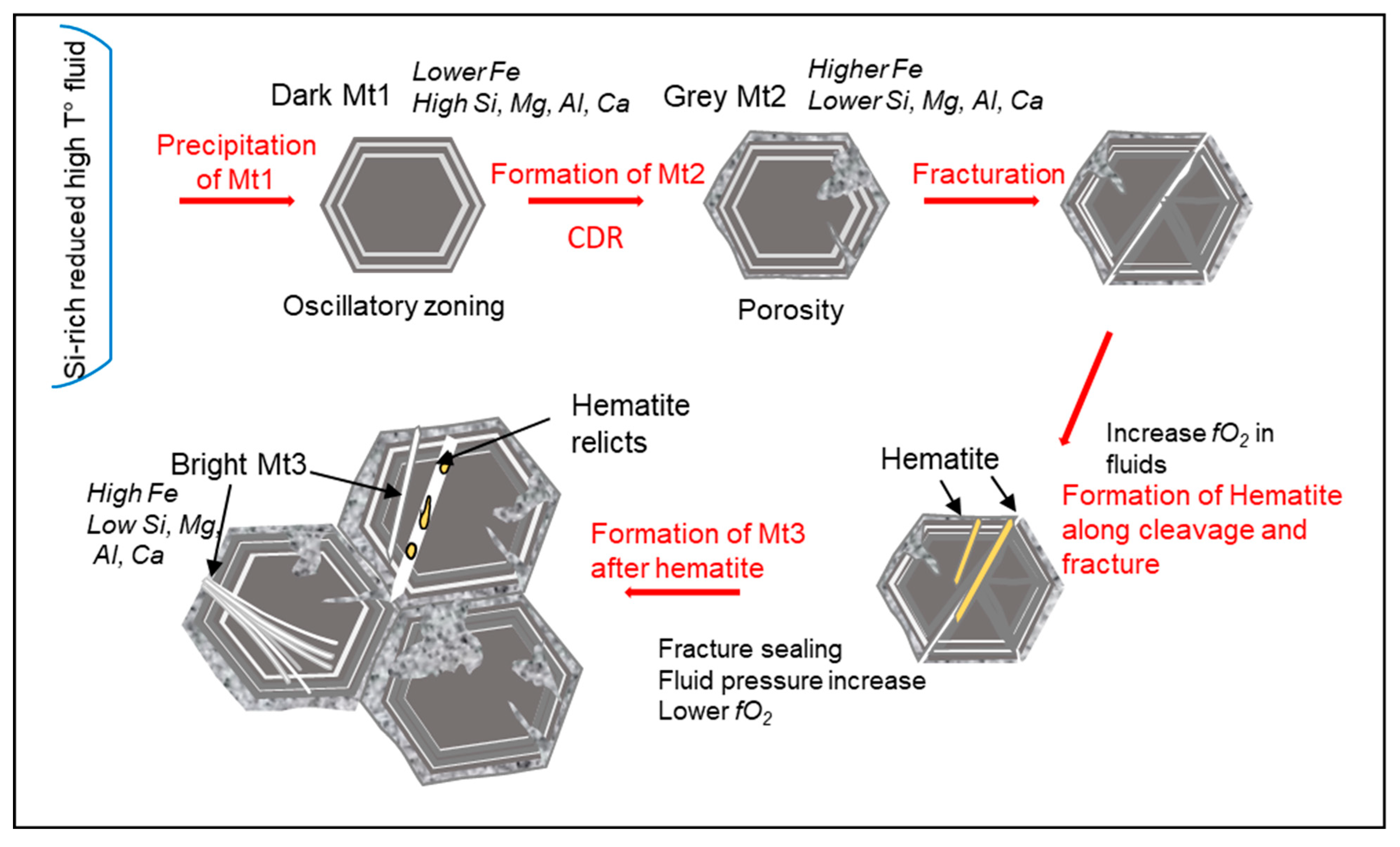
4.3. Dissolution–Reprecipitation Replacement of Mt1 by Mt2

Magnetite Mt1 was replaced by magnetite Mt2 mainly along grain margins. Mt1 magnetite is rich in minor elements (Si, Ca, and Al) compared to magnetite Mt2 (Table 2 and Figure 11). The relations between Mt1 and Mt2 are the following: (1) A close spatial relationship between Mt1 and Mt2 with a sharp boundary between Mt1 and Mt2 visible on BSE images and WDS X-ray maps (Figure 6, Figure 7 and Figure 8). IPF maps of composite Mt1 and Mt2 magnetite grains indicate a single-crystal domain shown by the same color, indicating the same orientation (Figure 15a,b). Similarly, the pole figures of selected areas in Mt1 and Mt2 show the coincidence of the crystallographic orientations of Mt1 and Mt2 (Figure 15c,d). This supports the inheritance of the crystallographic structure during the epitaxial growth of Mt2. (2) Porosity is locally developed in Mt2. (3) There is a sharp reaction front between Mt1 and Mt2 without diffusion, as shown in EMPA profiles (Figure 16c). Such compositional and textural characteristics suggest a fluid-induced replacement of Mt1 by Mt2 by a coupled dissolution–reprecipitation process (CDR) [5,47,48,49,50]. The CDR process allows the dissolution of early trace-element-rich Mt1 magnetite in the core and the precipitation of secondary Si-poor Mt2 magnetite at the rim. The presence of structural Si or nano-Si-rich inclusions in magnetite Mt1 would have caused a crystal lattice defect and/or deformation that would have facilitated its dissolution. Moreover, porosity would have facilitated the infiltration of hydrothermal fluid that, in turn, may have boosted the dissolution process. Coupled dissolution–reprecipitation evidenced here removed Si, Ca, and Mg from Mt1 magnetite near the reaction front and formed secondary Mt2 magnetite with lower trace-element content (type 1-CDR process in [5]).
Among the different factors that may control a dissolution–reprecipitation process, such as temperature, oxygen fugacity, and fluid composition [5,51,52,53], a change in fluid composition played here a major role in inducing the CDR process of magnetite Mt1/Mt2. The slight temperature decrease from Mt1 to Mt2 (Figure 13) may also have influenced the process. In contrast, the V content, similarly low (19–24 ppm, Table 2) in both Mt1 and Mt2, argues against a possible role of varying oxygen fugacity in the process.

4.4. Origin of Oscillatory Zoning in Magnetite Mt1

Oscillatory zoning of thin dark and light gray bands (in BSE) is observed in magnetite Mt1 and Mt-B large grains (Figure 8) and in the magnetite agglomerates (Figure 9). The decrease in brightness in BSE images indicates a lower concentration of trace elements with lower atomic numbers than Fe, such as Si, Al, and Ca. Oscillatory zoning is too fine to be analyzed, and no clear compositional variations could be demonstrated in EMPA profiles (Figure 16, zones B and D). Oscillatory zoning is generally interpreted as growth zoning under cyclical variation in fluid composition, temperature, or oxygen fugacity, which changes trace-element partitioning between magnetite and fluid [2,5,53]. The oscillatory zoning is parallel to the interface between Mt1 and Mt2, which likely results from a growth zoning under fluctuating fluid composition (Figure 8 and Figure 9). The preservation of oscillatory zoning requires crystal growth faster than the intracrystalline diffusion. Moreover, assuming that the thin dark and light gray bands may be similar in composition to Mt1 and Mt2 magnetite, respectively, we suggest that the oscillatory zoning would likely result from a fluctuating fluid composition rather than temperature or oxygen fugacity variation (see previous paragraph).

4.5. Origin of Magnetite Mt3 (Mushketovite)

Magnetite Mt3 has replaced the former platy hematite, now present as rare relicts, and is developed along cleavages and microfracture planes or crosscutting Mt1 and Mt2 magnetite grains (Figure 6). It is characterized by low concentrations of Si, Al, Mg, Ca, Mn, and Ti (Table 2, Figure 7, Figure 11 and Figure 16). The similarity between the crystal structures of magnetite and hematite controls the precipitation of magnetite and leads to the coincidence of orientation between the two minerals (Supplementary Figure S4). The pseudomorphic replacement of hematite by magnetite (mushketovitization) has been reported in many ore deposits in which mushketovite shows a platy morphology (e.g., [4,34] and references therein). It may result from two different processes: redox reactions by the reduction of Fe3+ to Fe2+ with the removal of oxygen and non-redox reactions by the addition of Fe2+ ions [54,55]. In the latter case, the number of Fe atoms increases, whereas in the redox process, the replacement of Fe3+ with Fe2+ causes a volume decrease calculated at 1.64% [4]. Magnetite Mt3 immediately adjacent to relict hematite shows microporosity, but porosity decreases with distance from hematite or in the bands without relict hematite. Thus, we propose that magnetite Mt3 likely formed via the redox transformation mechanism in a reducing environment compared to that prevailing for the formation of hematite.

5. Conclusions

This first study on the texture and chemistry of massive magnetite layers in amphibolites and micaschists confirms findings from previous studies on the disseminated and layered iron ore in micaschists from the same area, i.e., a Rapitan-type BIF mineralization formed in a back-arc basin, through iron precipitation and incorporation of terrigenous materials in the chemical precipitates of the original BIF. The protolith of the amphibolites was a basalt, typically interlayered with chemical and terrigenous marine sediments. Hydrothermal fluids formed and modified the iron ore.
Our findings support a formation in four steps (Figure 17): Step 1: The silician magnetite Mt1 likely formed in a rather reduced Si-rich environment, a hydrothermal volcano–sedimentary setting typical for BIF. The incorporation of structural or nano-Si-rich inclusions may have caused lattice defects or deformation promoting fluid circulation and alteration of the magnetite grains. Step 2: A fluid-induced coupled dissolution of Mt1 and precipitation of Mt2 (CDR process) is supported by a close spatial relationship, sharp compositional boundaries, the similar crystallographic structure of Mt1 and Mt2, and porosity in Mt2. Porosity promotes the infiltration of hydrothermal fluids, accelerating the CDR process. Step 3: Microfracturing increasing the permeability led to the penetration of a more oxidized fluid along cleavage planes and the formation of platy hematite. By increasing the contact between the fluid and the magnetite grain, microfracturing allows an acceleration of the oxidation process and dissolution of magnetite. Step 4: Finally, after progressive sealing of the fractures, mushketovite Mt3 formed after hematite from a more reduced fluid composition by a redox transformation supported by the volume decrease. Deformation can be attributed to the two latter steps.

Supplementary Materials

The following supporting information can be downloaded at: https://www.mdpi.com/article/10.3390/min15020137/s1, Figure S1: WDS X-ray maps of selected elements in a magnetite grain from sample TAK-Z3. Figure S2: Discrimination diagram V vs Ti for the Takab magnetite. Figure S3. Ca vs. (Si + Al) plot of magnetite Mt1 and amphibole from sample TAK-Z1. Figure S4: Pole figures of magnetite Mt3 and relict hematite. Table S1: Composition of feldspar in amphibolite host rock and iron ore from Takab. Table S2: Fe, O, and trace-element composition of magnetite from the Takab iron ore samples. Table S3: Average formation temperature for the Takab magnetite.

Author Contributions

Conceptualization, C.W. and B.O.; investigation, C.W., O.B., N.R. and B.O.; project administration, C.W. and B.O.; resources, C.W., B.O., G.N., M.H. and I.M.; supervision, C.W.; validation, C.W., O.B. and N.R.; visualization, C.W., G.N. and M.H.; writing—original draft, C.W.; writing—review and editing, C.W., B.O., G.N. and M.H. All authors have read and agreed to the published version of the manuscript.

Funding

We thank the Institute of Advanced Sciences of Basic Science and University of Zanjan, Zanjan, for logistic support during fieldwork and the stay of BO in Zanjan. Campus France and the French embassy (Gundishapur project No. 40624TK) are thanked for financing the stay of BO at IASBS, Zanjan. The institute ISTeP of Sorbonne Université is thanked for financial support of the analyses through the French National TRIGGER project, French–Iranian cooperation.

Data Availability Statement

The original contributions presented in this study are included in the article and Supplementary Materials.

Acknowledgments

L. Reisberg (CRPG, Vandoeuvre-lès-Nanvy, France) is kindly acknowledged for a thorough review and English revision of the manuscript. We thank three anonymous reviewers for their helpful comments.

Conflicts of Interest

The authors declare no conflicts of interest.

References

  1. Dupuis, C.; Beaudouin, G. Discriminant diagrams for iron oxide trace element finger printing of mineral deposit types. Miner. Deposita 2011, 46, 319–335. [Google Scholar] [CrossRef]
  2. Dare, S.A.S.; Barnes, S.-J.; Beaudoin, G.; Méric, J.; Boutroy, E.; Potvin-Doucet, C. Trace elements in magnetite as petrogenetic indicators. Miner. Deposita 2014, 49, 785–796. [Google Scholar] [CrossRef]
  3. Nadoll, P.; Angerer, T.; Mauk, J.L.; French, D.; Walshe, J. The chemistry of hydrothermal magnetite: A review. Ore Geol. Rev. 2014, 16, 1–32. [Google Scholar] [CrossRef]
  4. Hu, X.; Chen, H.; Beaudouin, G.; Zhang, Y. Textural and compositional evolution of iron oxides at Mina Justa (Peru): Implications for mushketovite and formation of IOGC deposits. Am. Mineral. 2020, 105, 397–408. [Google Scholar] [CrossRef]
  5. Huang, X.W.; Beaudoin, G. Textures and chemical compositions of magnetite from iron oxide copper-gold (IOCG) and Kiruna-type iron oxide-apatite deposits and their implications for ore genesis and magnetite classification schemes. Econ. Geol. 2019, 114, 953–979. [Google Scholar] [CrossRef]
  6. Zhang, Y.; Hollings, P.; Shao, Y.; Li, D.; Chen, H.; Li, H. Magnetite texture and trace-element geochemistry fingerprint of pulsed mineralization in the Xinqiao Cu-Fe-Au deposit, Eastern China. Am. Mineral. 2020, 105, 1712–1723. [Google Scholar] [CrossRef]
  7. Liang, P.; Wu, C.; Hu, X.; Xie, Y. Textures and geochemistry of magnetite: Indications for genesis of the Late Paleozoic Laoshankou Fe-Cu-Au deposit, NW China. Ore Geol. Rev. 2020, 124, 103632. [Google Scholar] [CrossRef]
  8. Honarmand, M.; Nabatian, N.; Wagner, C.; Monsef, I.; Delpech, G.; Bayon, G.; Orberger, B. Late Ediacaran iron formation, NW Iran: Origin, depositional age and tectonic/climate significance. Precambrian Res. 2024, 406, 107382. [Google Scholar] [CrossRef]
  9. Karimpour, M. Applied Economic Geology; Javid Publication: Mashhad, Iran, 1989; 404p. [Google Scholar]
  10. Nabatian, G.; Rastad, E.; Neubauer, F.; Honarmand, M.; Ghaderi, M. Iron and Fe-Mn mineralisation in Iran: Implications for Tethyan metallogeny. Aust. J. Earth Sci. 2015, 62, 211–241. [Google Scholar] [CrossRef]
  11. Tuck, C.C. Iron ore. In Mineral Commodity Summaries; USGS Reports; USGS Reports; National Minerals Information Center: Reston, VA, USA, 2023. [Google Scholar]
  12. Foster, H.; Jafarzadeh, A. The Bafq mining district in Central Iran—A highly mineralized Infracambrian volcanic field. Econ. Geol. 1994, 89, 1697–1721. [Google Scholar] [CrossRef]
  13. Mazaheri, S.A.; Andrew, A.S.; Chenhall, B.E. Petrological Studies of Sangan Iron Ore Deposit; Center for Isotope Studies Research Report: Sydney, NSW, Australia, 1994; pp. 48–52. [Google Scholar]
  14. Daliran, F. Kiruna-Type Iron Oxide-Apatite Ores and Apatitites of the Bafq District, Iran, with an Emphasis on the REE Geochemistry of Their Apatites. In Hydrothermal Iron Oxide Copper Gold and Related Deposits. A Global Perspective; Porter, T.M., Ed.; PGC Publishing: Adelaide, SA, Australia, 2002; Volume 2, pp. 303–320. [Google Scholar]
  15. Daliran, F.; Stosch, H.G.; Williams, P.; Jamli, H.; Dorri, M.B. Lower Cambrian Iron Oxide-Apatite-REE (U) Deposits of the Bafq District, East-Central Iran. In Exploring for Iron Oxide Copper-Gold Deposits: Canada and Global Analogues; Corriveau, L., Mumin, H., Eds.; Geological Association of Canada Short Course Notes: St John’s, NL, Canada, 2010; Volume 20, pp. 143–155. [Google Scholar]
  16. Alavi, M. Sedimentary and structural characteristics of the Paleo-Tethys remnants in northeastern Iran. GSA Bull. 1991, 103, 983–992. [Google Scholar] [CrossRef]
  17. Berberian, M.; King, G.C.P. Towards a paleogeography and tectonic evolution of Iran. Can. J. Earth Sci. 1981, 18, 210–265. [Google Scholar] [CrossRef]
  18. Jafari, A.; Karimpour, M.H.; Mazaheri, S.A.; Shafaroudi, A.M.; Ren, M. Geochemistry of metamorphic rocks and mineralization in the Gol-Gohar iron ore deposit (No. 1), Sirjan, SE Iran: Implications for Paleotectonic setting and ore genesis. J. Geochem. Explor. 2019, 205, 106330. [Google Scholar] [CrossRef]
  19. Nabatian, G.; Ghaderi, M.; Daliran, F.; Rashidnejad-Omran, N. Sorkhe-Dizaj iron oxide-apatite ore deposit in the Cenozoic Alborz-Azarbaijan magmatic belt, NW Iran. Resour. Geol. 2013, 63, 42–56. [Google Scholar] [CrossRef]
  20. Nabatian, G.; Li, X.-H.; Honarmand, M.; Melgarejo, J.C. Geology, mineralogy and evolution of iron skarn deposits in the Zanjan district, NW Iran: Constraints from U-Pb dating, Hf and O isotope analyses of zircons and stable isotope geochemistry. Ore Geol. Rev. 2017, 84, 42–66. [Google Scholar] [CrossRef]
  21. Sarjoughian, F.; Habibi, H.; Lentz, D.R.; Azizi, H.; Esna-Ashari, A. Magnetite compositions from the Baba Ail iron deposit in the Sanandaj-Sirjan zone, western Iran: Implications for ore genesis. Ore Geol. Rev. 2020, 126, 103728. [Google Scholar] [CrossRef]
  22. Maanijou, M.; Khodaei, L. Mineralogy and electron microprobe studies of magnetite in the Sarab-3 iron Ore deposit, southwest of the Shahrak mining region (east Takab). J. Econ. Geol. 2018, 10, 267–293. (In Persian) [Google Scholar]
  23. Maanijou, M.; Salemi, R. Mineralogy, chemistry of magnetite and genesis of Korkora-1 iron deposit, east of Takab, NW Iran. J. Econ. Geol. 2014, 6, 355–374. (In Persian) [Google Scholar]
  24. Ghaderi Piraghoum, Z.; Kouhestani, H.; Tofighi, F. Geology, geochemistry and genesis of the Kosaj Fe occurrence, Takab‒Takht-e Soleiman‒Angouran metallogenic zone, SW Zanjan. Adv. Appl. Geol. 2020, 10, 294–313, (In Persian with English abstract). [Google Scholar]
  25. Pourmohammad, F.; Kouhestani, H.; Azimzadeh, A.M.; Nabatian, G.; Mokhtari, M.A.A. Mianaj iron occurrence, southwest of Zanjan: Metamorphosed and deformed volcano-sedimentary type of mineralization in Sanandaj-Sirjan zone. Sci. Q. J. Geosci. 2019, 28, 161–174, (In Persian with English abstract). [Google Scholar]
  26. Biparva, M. Geochemistry, Mineralogy and Genesis of Fe Deposits, East of Takab (Halab, Mianaj and Quzijan Villages). Master’s Thesis, Department of Geology, Shahid Beheshti University, Teheran, Iran, 2013. Unpublished (In Persian with English abstract). [Google Scholar]
  27. Fereiduni, Z. Geology, Mineralogy and Geochemistry of Halab Iron Mineralization, SW Zanjan. Master’s Thesis, Department of Geology, University of Zanjan, Zanjan, Iran, 2017. Unpublished (In Persian with English abstract). [Google Scholar]
  28. Wagner, C.; Villeneuve, J.; Boudouma, O.; Rividi, N.; Orberger, B.; Nabatian, G.; Honarmand, M.; Monsef, I. In Situ Trace Element and Fe-O Isotope Studies on Magnetite of the Iron-Oxide Ores from the Takab Region, North Western Iran: Implications for Ore Genesis. Minerals 2023, 13, 774. [Google Scholar] [CrossRef]
  29. Hassanzadeh, J.; Stockli, D.F.; Horton, B.K.; Axen, G.J.; Stockli, L.D.; Grove, M.; Schmitt, A.K.; Walker, J.D. U-Pb zircon geochronology of late Neoproterozoic-early Cambrian granitoids in Iran: Implications for paleogeography, magmatism, and exhumation history of Iranian basement. Tectonophysics 2008, 451, 71–96. [Google Scholar] [CrossRef]
  30. Hajialioghli, R.; Moazzen, M.; Jahangiri, A.; Oberhansli, R.; Mocek, B.; Altenberger, U. Petrogenesis and tectonic evolution of metaluminous sub-alkaline granitoids from the Takab complex, NW Iran. Geol. Mag. 2011, 148, 250–268. [Google Scholar] [CrossRef]
  31. Moazzen, M.; Hajialioggli, R. Zircon SHRIMP Dating of Mafic Migmatites from NW Iran: Reporting the Oldest Rocks from the Iranian Crust. In Proceedings of the 5th Annual Meeting AOGS, Busan, Korea, 16–20 June 2008. [Google Scholar]
  32. Babakhani, A.R.; Ghalamghash, J. Explanatory Text of Takht-e-Soleiman. In Geological Quadrangle Map 1:100000, No.5463; Geological Survey of Iran: Tehran, Iran, 2005. (In Persian) [Google Scholar]
  33. Till, J.L.; Moskowitz, B.M. Deformation microstructures and magnetite texture development in synthetic shear zones. Tectonophysics 2014, 629, 211–223. [Google Scholar] [CrossRef]
  34. Hu, X.; Xiao, B.; Jiang, H.; Huang, J. Magnetite texture and trace element evolution in the Shaquanzi Fe-Cu deposit, Eastern Tianshan, NW China. Ore Geol. Rev. 2023, 154, 105306. [Google Scholar] [CrossRef]
  35. Nielsen, R.L.; Forsythe, L.M.; Gallahan, W.E.; Fisk, M.R. Major element and trace element magnetite-melt equilibria. Chem. Geol. 1994, 117, 167–191. [Google Scholar] [CrossRef]
  36. Toplis, M.J.; Caroll, M.R. An experimental study of oxygen fugacity on Fe-Ti oxide stability, phase relations, and mineral-melt equilibria in ferro-basaltic systems. J. Petrol. 1995, 36, 1137–1170. [Google Scholar] [CrossRef]
  37. Deditius, A.P.; Reich, M.; Simon, A.C.; Suvorova, A.; Knipping, J.; Roberts, M.P.; Rubanov, S.; Dodd, A.; Saunders, M. Nanogeochemistry of hydrothermal magnetite. Contrib. Mineral. Petrol. 2018, 173, 46. [Google Scholar] [CrossRef]
  38. Xu, H.; Shen, Z.; Konishi, H. Si-magnetite nano-precipitates in silician magnetite from banded iron formation: Z-contrast imaging and ab-initio study. Amer. Mineral. 2014, 99, 2196–2202. [Google Scholar] [CrossRef]
  39. Ciobanu, C.L.; Verdugo-Ihl, M.R.; Slattery, A.; Cook, N.J.; Ehrig, K.; Courtney-Davies, L.; Wade, B.P. Silician Magnetite: Si–Fe-Nanoprecipitates and Other Mineral Inclusions in Magnetite from the Olympic Dam Deposit, South Australia. Minerals 2019, 9, 311. [Google Scholar] [CrossRef]
  40. Canil, D.; Lacourse, T. Geothermometry using minor and trace elements in igneous and hydrothermal magnetite. Chem. Geol. 2020, 541, 119576. [Google Scholar] [CrossRef]
  41. Huberty, J.M.; Konishi, H.; Heck, P.R.; Fournelle, J.H.; Valley, J.W.; Xu, H. Silician magnetite from the Dales Gorge Member of the Brockman Iron Hamersley Group, Western Australia. Am. Mineral. 2012, 97, 26–37. [Google Scholar] [CrossRef]
  42. Whittaker, E.J.W.; Muntus, R. Ionic radii for use in geochemistry. Geochim. Cosmochim. Acta 1970, 34, 945–956. [Google Scholar] [CrossRef]
  43. Hu, X.; Chen, H.; Zhang, W. Texture and composition of magnetite in the Duotoushan deposit, NW China: Implications for ore genesis of Fe-Cu deposits. Min. Mag. 2020, 84, 398–411. [Google Scholar] [CrossRef]
  44. Shimazaki, H. On the occurrence of silician magnetite. Resour. Geol. 1998, 48, 23–29. [Google Scholar] [CrossRef]
  45. Ohkawa, M.; Miyahara, M.; Ohta, E.; Hoshino, K. Silicon-substituted magnetite and accompanying iron oxides and hydroxides from the Kumano mine, Yamaguchi Prefecture, Japan: Reexamination of the so-called maghemite (g-Fe2O3). J. Mineral. Petrol. Sci. 2007, 102, 182–193. [Google Scholar] [CrossRef]
  46. Sun, S.; Li, Y.-L. Microstructures, crystallography and geochemistry of magnetite in 2500 to 2200 million-year old banded iron formation from South Africa, Western Australian and North China. Prec. Res. 2017, 298, 292–305. [Google Scholar] [CrossRef]
  47. Putnis, A. Mineral replacement reactions. In Thermodynamics and Kinetics of Water-Rock Interaction; Oelkers, E., Schott, J., Eds.; Reviews in Mineralogy & Geochemistry, Mineralogical Society of America: Chantilly, VA, USA, 2009; Volume 70, pp. 87–124. [Google Scholar]
  48. Putnis, A. Transient porosity resulting from fluid-mineral interaction and its consequences. In Pore-Scale Geochemical Processes; Steefel, C.I., Emmanuel, S., Anovitz, L.M., Eds.; Reviews in Mineralogy & Geochemistry, Mineralogical Society of America: Chantilly, VA, USA, 2009; Volume 80, pp. 1–23. [Google Scholar]
  49. Altree-Williams, A.; Pring, A.; Ngothai, Y.; Brugger, J. Textural and compositional complexities resulting from coupled dissolution-reprecipitation reactions in geomaterials. Earth Sci. Rev. 2015, 150, 628–651. [Google Scholar] [CrossRef]
  50. Hu, H.; Li, J.W.; Lentz, D.; Ren, Z.; Zhao, X.F.; Deng, X.D.; Hall, D. Dissolution-re precipitation process of magnetite from the Chengchao iron deposit: Insights into ore genesis and implication for in-situ chemical analysis of magnetite. Ore Geol. Rev. 2014, 57, 393–405. [Google Scholar] [CrossRef]
  51. Hu, H.; Lentz, D.; Li, J.-W.; McCarron, T.; Zhao, X.-F.; Hall, D. Reequilibration processes in magnetite from iron skarn deposits. Econ. Geol. 2015, 110, 1–8. [Google Scholar] [CrossRef]
  52. Yin, S.; Ma, C.Q.; Robinson, P.T. Textures and high field strength elements in hydrothermal magnetite from a skarn system: Implications for coupled dissolution-reprecipitation reactions. Am. Miner. 2017, 102, 1045–1056. [Google Scholar] [CrossRef]
  53. Zhang, S.; Chen, H.; Xiao, B.; Zhao, L.; Hu, X.; Li, J.; Gong, L. Textural and chemical evolution of magnetite from the Paleozoic Shuanglong Fe-Cu deposit: Implications for tracing ore-forming fluids. Am. Miner. 2023, 108, 178–191. [Google Scholar] [CrossRef]
  54. Ohmoto, H. Nonredox transformations of magnetite-hematite in hydrothermal systems. Econ. Geol. 2003, 98, 157–161. [Google Scholar] [CrossRef]
  55. Mücke, A.; Cabral, A.R. Redox and non-redox reactions of magnetite and hematite in rocks. Geochemistry 2005, 65, 271–278. [Google Scholar] [CrossRef]
Figure 1. Tectonic and structural map of Iran (after [10]). The red star indicates the location of the Takab study area (Takab town GPS coordinates are 36°24′2″ E and 47°6′42″ E). The black boxes correspond to the locations of different types of iron ore deposits in Iran. Zagros, Zagros ranges; KRSZ, Kermanshah Radiolarites subzone; SSZ, Sanandaj–Sirjan zone; UD, Urumieh–Dokhtar magmatic arc; the Central Iranian microcontinent includes Yadz, Posht-e-Badam block (PB), Tabas, and Lut blocks; AMB, Alborz magmatic arc; KTZ, Khazar–Talesh–Ziveh structural zone; CIZ, Central Iranian zone; Sistan, East Iran ranges; Makran, Makran zone; KD, Kopeh–Dagh ranges; Zabol, Zabol area; CMR, Cenozoic magmatic rocks [10].
Minerals 15 00137 g001
Figure 2. Simplified geological map of the Takab area modified after [8]. The marked area (47°23′51″ E to 47°25′39″ E longitude and 36°29′13″ N to 36°30′03″ N latitude) limits the location of the Takab iron ore samples from previous studies (yellow circles: banded, nodular, and disseminated iron ore, [8,28]) and from this study (yellow stars: massive iron ore).
Minerals 15 00137 g002
Figure 3. (af) Field photographs of the outcrops of the Takab iron ore deposit. (g,h) Close-up view of the amphibolite hosting massive magnetite ore.
Minerals 15 00137 g003
Figure 4. Amphibolite mineralogy: optical photomicrographs (a) in plane-polarized light and (c,e) in cross-polarized light; backscattered images (b,d,fh). (a) Actinolite and minor biotite alternating with quartz and feldspar transparent patches; (b) actinolite with a Mg-rich core; interstitial calcite crystal also shown in (c) and accessory apatite. (d) Epidote and chlorite developed in biotite. (eh) Accessory titanite, barite, allanite, and pyrite.
Minerals 15 00137 g004
Figure 5. Hand specimen (a) and enlarged views of the massive magnetite ore from Takab. (b) Thin section (3.8 cm x 2.5 cm), (c) close-up view of the contact between the amphibolite and the magnetite ore, and (d) BSE image of the area marked in (c) showing the amphibole Mg-rich core. (e,f) Optical photomicrographs in cross-polarized light of prismatic, fibrous, and acicular amphibole crystals. (f) Rosette-shaped interstitial chlorite.
Minerals 15 00137 g005
Figure 6. Morphology and textures of magnetite. BSE image of magnetite grains from sample TAK-Z3. (a) Dark gray magnetite Mt1 is surrounded by lighter gray magnetite Mt2 (bottom right), which locally invaded Mt1 (upper left). Magnetite Mt3 forms bright bands, which may host relict hematite (Hem). (b) Inverse pole figure (IPF) of relict hematite phases (white arrows) in two Mt3 bands outlined by the yellow dashed lines (sample TAK-Z1). Different relict hematite patches within one single Mt3 band display similar colors, indicating that hematite patches have similar crystallographic orientation and, thus, represent a unique hematite band. (c) Reflected light. Enlarged view of an Mt3 band (outlined by the yellow dashed lines) with relict hematite (bright patches) undergoing transformation in Mt3 (red arrows).
Minerals 15 00137 g006
Figure 7. BSE image (a) and WDS X-ray maps of selected elements in a magnetite grain from sample TAK-Z1 (bf). Magnetite Mt1 contains higher Si, Al, Mg, and Ca than magnetite Mt2. Mt3 bands have the highest Fe and the lowest Si, Al, Mg, and Ca contents. The yellow rectangle corresponds to the zone detailed in Figure 8. The red arrow is precised in Figure 8.
Minerals 15 00137 g007
Figure 8. Detailed BSE image (a) and WDS X-ray maps of selected elements (bf) in a magnetite grain from sample TAK-Z1 showing dark magnetite Mt1 (D) and the different subzones of gray magnetite Mt2 (zones A, B, C). Oscillatory zoning is visible in Mt1 and Mt2-B. The total grain is shown in Figure 7. The red arrow limits the different zones of magnetite Mt2, see text for details.
Minerals 15 00137 g008
Figure 9. (ad) WDS X-ray maps of selected elements in an aggregate of smaller magnetite grains from sample TAK-Z4 with compositional and zoning characteristics like to those of large magnetite grains (Figure 8).
Minerals 15 00137 g009
Figure 10. Inverse pole figure IPF Y (a) and pole figures (b,c) of magnetite from sample TAK-Z1. The dotted lines delimit the larger Mt3 band of Figure 6b. Abrupt changes in color reflect changes in orientation across grain boundaries. Wavy misorientation reflects intragrain deformation. In the latter case, the pole figure shows dispersed points along circle girdles (subset 2) compared to the clustered points of uniform intragrain orientation (subset 1). H: hematite.
Minerals 15 00137 g010
Figure 11. Binary plots of selected elements in magnetite from Takab, sample TAK-Z3. (a) [Si + Al + Mg + Ca + Mn] vs. Fe (wt. %) and (b) Ca vs. [Si + Al + Mg] (ppm), showing high trace-element and low Fe contents in magnetite Mt1 compared to magnetite Mt2. Magnetite Mt3 has the lowest trace-element and the highest Fe contents. (c) Si and Al vs. Fe3+ and (d) [Ca + Mg + Mn] vs. Si diagrams (in apfu) show the negative correlation of Fe3+ with Si and Al, possibly indicating the incorporation of Si in the magnetite structure by substitution for Fe3+, while Si is positively correlated with Ca, Mg, and Mn as valence-state species related to the substitution. Blue circles, Mt1; yellow squares, Mt2; filled red triangles, non-porous Mt3; and red open triangles, porous Mt3. Calculation of Fe2+/Fe3+ partitioning explained in Supplementary Table S2.
Minerals 15 00137 g011
Figure 12. Discrimination diagram of Fe/(Mg + Mn + Al) vs. Ti. The different magnetite types from samples TAK-Z1 and TAK-Z3 plot in the hydrothermal domain. The boxes outline the domains of banded (B), nodular (N), and disseminated (D) magnetite previously studied [28]. Hydrothermal and magmatic domains are after [34].
Minerals 15 00137 g012
Figure 13. Approximate temperatures of formation of magnetite. Temperature reference fields are after [3,38]. The boxes outline the domains of banded (B), nodular (N), and disseminated (D) iron ore samples previously studied [28].
Minerals 15 00137 g013
Figure 14. Calculated formation temperatures for Takab magnetite show a decreasing trend from magnetite Mt1 and Mt2 to magnetite Mt3. The temperatures were calculated using the T°Mg-mag thermometer of [40]. The calculated T° values have an uncertainty of about ±60 °C. In sample TAK-Z3, Mt3p corresponds to porous Mt3 adjacent to relict hematite. Mt3 was not observed in sample TAK-Z4. The points correspond to the total analyses in Supplementary Table S2 and calculated temperatures in Supplementary Table S3. (X): mean values.
Minerals 15 00137 g014
Figure 15. Enlarged BSE image (a) and inverse pole figure IPF Y (b) of Mt1 and Mt2 adjacent zones in a magnetite grain from sample TAK-Z1, and pole figures (c,d) of selected areas corresponding to Mt1 and Mt2 showing a similar orientation of Mt1 and Mt2 in favor of a CDR process (see text).
Minerals 15 00137 g015
Figure 16. BSE images of the magnetite from sample TAK-Z1 (a) and enlarged view of the yellow contoured zone (b). In (b), the red arrow indicates the EMPA element profile (c) through the different magnetite zones Mt1, Mt2, and Mt3. The multi-element profiles show the difference in composition and the sharp contact between the different magnetite types. WDS X-ray maps of the same area are given in Figure 7 and Figure 8. See text for explanations of the different zones A-E.
Minerals 15 00137 g016
Figure 17. Schematic illustration of the multiple processes involved in the formation of magnetite from the Takab iron ore deposit. CDR: coupled dissolution–reprecipitation process. Dark, gray, and bright magnetite as defined on BSE images.
Minerals 15 00137 g017
Table 1. Composition (in wt. %) of amphibole from Takab host amphibolite and iron ore.
HostIron Ore
ActinoliteTrMhbActinolite
corecoreacicular crystals core
SiO2 54.4451.8350.853.955.9755.9757.3249.3647.3448.4552.5551.7555.93
TiO20.120.110.080.1000.050.370.410.430.050.060.03
Al2O31.512.973.611.272.852.853.027.427.638.052.12.833.81
Cr2O30.040.110.050.060.030.030.010.130.130.140.0300.02
FeO15.9618.0118.3415.65.95.91.9713.9316.3613.916.8117.023.82
MnO0.190.120.230.160.10.10.10.50.380.570.120.120
MgO13.9512.5312.3114.0420.2120.2122.5313.7912.413.4913.4612.9720.83
CaO12.0211.6511.8712.33121212.6311.2811.5711.3312.1112.3612.46
Na2O0.450.670.840.381.181.181.131.51.281.480.490.641.38
K2O0.080.170.160.10.260.260.080.160.340.150.150.130.17
Total98.7698.1698.397.9598.598.598.8598.4497.849897.8797.8898.45
mg#61.155.654.761.886.186.195.464.157.763.65957.890.7
Tr = tremolite, Mhb = magnesio hornblende. mg#= 100*Mg/(Mg+Fe).
Table 2. Fe and O (wt. %) minor- and trace-element (ppm) contents of magnetite from Takab.
Sample TAK-Z1TAK-Z1TAK-Z1TAK-Z4TAK-Z4
Mt type Mt1Mt2Mt3Mt1Mt2
n analyses 1241086
Fe (wt. %)Average68.069.870.867.669.6
Range66.1–69.469.3–70.469.9–71.367.2–68.769.0–70.1
O (wt. %)Average29.428.628.529.128.7
Range29.0–29.728.2–28.828.0–29.128.0–29.627.8–29.1
SiAverage11,017433621499423550
sd11074091951444397
DL = 11Range8899–127793846–484011–4268274–11,9413149–4045
TiAverage1308626293104
sd61352012018
DL = 4Range51–27637–126BDL-63 (2)149–47473–106
AlAverage248910312752321985
sd4797694364173
DL = 12Range1428–3103947–1120187–4341617–2773818–1301
MnAverage262227261279223
sd26591075427
DL= 5Range198–289161–305166–519198–368193–273
MgAverage1263410341225382
sd32013426378131
DL = 19Range807–1882234–560BDL-71 (4)825–1794205–553
CaAverage2677128931327991192
sd58510995720294
DL = 3Range1606–35291127–1349194–4841760–38211018–1155
VAverage221934ndnd
sd1056
DL = 9Range13–4312–2422–42
Sample TAK-Z3TAK-Z3TAK-Z3TAK-Z3
Mt type Mt1Mt2Mt3 porousMt3
n analyses 2310813
Fe (wt. %)Average68.269.77171.1
Range67.5–69.269.5–70.270.1–71.570.4–71.8
O (wt. %)Average29.429.028.728.8
Range28.9–29.928.6–29.228.3–29.728.4–29.5
SiAverage118065430587432
sd1231936445274
DL = 11Range9769–13,7853949–717012–87055–884
TiAverage14356938
sd6113522
DL = 4Range38–24637–82BDL-17 (2)8–65
AlAverage27811190278239
sd50025295104
DL = 12Range1745–3480759–1621175–468105–519
MnAverage222240198181
sd23324545
DL= 5Range181–262196–276148–292101–261
MgAverage12727754262
sd3082202428
DL = 19Range614–1738342–1064BDL-70 (2)18–89
CaAverage28661661473416
sd521353213179
DL = 3Range1966–35751150–2226249–824228–797
VAverage2421nd27
sd108 7
DL = 9Range11–3911–30 22–42
Ni and Cu are not reported as their contents are below or close to the detection limits (DL = 12 and 8 ppm, respectively). BDL = below detection limit. (n) = number of analyses below the detection limit. nd = not determined. sd = standard deviation.
Disclaimer/Publisher’s Note: The statements, opinions and data contained in all publications are solely those of the individual author(s) and contributor(s) and not of MDPI and/or the editor(s). MDPI and/or the editor(s) disclaim responsibility for any injury to people or property resulting from any ideas, methods, instructions or products referred to in the content.

