Abstract
Rare earth elements are gaining significant importance in the scientific and technological fields for their exciting physical properties and characteristics. The aim of the present study was to determine rare earth elements (REEs) in geological ores found in the Northern Areas of Pakistan. We present the application of laser-induced breakdown spectroscopy (LIBS) and laser ablation time-of-flight mass spectrometry (LA-TOF-MS) for the elemental analysis of geological ore samples containing REEs. The laser-induced plasma plume exhibits a wide array of emission lines, including those of rare earth elements such as Ce, La, and Nd. Furthermore, the spectral range, from 220 nm to 970 nm, encompasses emission lines from C, Fe, Ti, Na, Mg, Si, and Ca. The qualitative analysis of the constituent elements in the samples was performed by comparing the LIBS spectrum of the unknown sample with that of the spectroscopically pure rare earth elements (La2O3, CeO2, and Nd2O3, with 99.9% metals basis) recorded under the same experimental conditions. The quantitative analysis was performed using the calibration-free laser-induced breakdown spectroscopy (CF-LIBS), LA-TOF-MS, and energy-dispersive X-ray (EDX) techniques. The results obtained by CF-LIBS were found to be in good agreement with those obtained using the LA-TOF-MS and EDX analytical techniques. LIBS is demonstrated to yield a quick and reliable qualitative and quantitative analysis, of any unknown geological sample, comparable to that of the other analytical techniques.
1. Introduction
Rare earth elements (REEs) comprise elements with atomic numbers 57–71, encompassing La to Lu, as well as two additional elements, scandium (Sc) and yttrium (Y). These elements are classified as REEs due to their notable physical properties and chemical characteristics, which have contributed to their increasing significance in the scientific and technological domains. They are widely used in the study of volcanic rocks, sedimentology, and in the processes of oceanography [1,2,3,4]. The application of these elements in geochemistry has been extensive, primarily due to their ability to provide insights into crucial geochemical and petrographic processes. In the field of geochemistry, these elements play a role in understanding the intricate structure of chemical elements within rocks and minerals. Additionally, in petrography, they contribute to the systematic classification and accurate description of various rock types. By understanding their distribution in rocks and minerals, and utilizing them under varying environmental conditions, researchers can effectively investigate and unravel significant aspects, such as the examination of bauxite-heavy mineral concentrates [5]. The economic interest of REEs is obvious, since they play an important role in several scientific fields and industrial applications. REEs are being used in defense and in renewable energy production, as well as in advanced digital products such as cell phones, magnets, fiber optic cables, television, hybrid cars, and medical imaging. Rare earth elements find applications in advanced technologies, including fluorescent lamps, radar screens, and plasma displays. They are also utilized in auto exhaust absorption catalysts and high-tech glasses [6]. Rare earth metals and their alloys are also used in the manufacturing of wind turbines, electric vehicles, rechargeable batteries, radar systems, and laser crystals [7,8]. Hence, there is a strong demand for conducting qualitative and quantitative analyses of these REEs found in ores, as it is crucial for their incorporation into industrial products.
Several analytical techniques, including inductively coupled plasma mass spectrometry (ICP-MS), inductively coupled plasma optical emission spectrometry (ICP-OES), neutron activation analysis (NAA), X-ray fluorescence (XRF), wavelength-dispersive XRF (WD-XRF) spectrometers, or energy-dispersive XRF (ED-XRF) instruments, are being used to quantify REEs [9,10,11]. Laser-induced breakdown spectroscopy (LIBS) is a versatile emerging analytical technique used to analyze the chemical composition of a wide range of materials, including metallic alloys, dielectric materials, powders, biological substances, minerals, aerosols, as well as micro and nanoparticles. Being a quasi-non-destructive technique, LIBS offers the advantage of high sensitivity, enabling it to achieve a low limit of detection (LOD) [12,13]. Furthermore, one of the unique features of LIBS is the remote and stand-off option for inaccessible objects. Although LIBS is a potential technique for multi-elemental analysis, along with high resolution, it has some limitations, including accuracy and precision. Obtaining reliable results using the LIBS technique depends on various factors, including self-absorption, laser pulse energy, delay time, intensity calibration, and the efficiency of the CCD/ICCD detectors. These elements significantly impact the accuracy and precision of the technique. The analysis of liquid samples by LIBS is less preferred due to some additional complications such as splashing, surface ripples, quenching of emitted intensity, and a shorter plasma lifetime [14,15]. The working principle of LIBS is explained in several books and review articles [16,17,18,19]. In brief, the laser beam is focused on the surface of the material intended for analysis, causing radiation energy to interact specifically with the target material. This interaction initiates the process of material evaporation, followed by dissociation and ionization of the resulting vapor, ultimately forming plasma. As the plasma gradually cools down, it emits light naturally, which is collected and subjected to analysis using a spectrometer.
A variety of sample types, including monazite sand, coal ash, composites with oxide matrices, astronomical specimens, and phosphorite, were the focus of certain previous studies on rare earth elements. For instance, Abedin et al. [20] used the LIBS technique to analyze the raw monazite sands, collected from the beaches of Bangladesh, and detected several rare earth elements, such as cerium, lanthanum, praseodymium, neodymium, yttrium, ytterbium, gadolinium, dysprosium, and erbium, in addition to other metallic elements, such as zirconium, chromium, titanium, magnesium, manganese, niobium, and aluminum. Phuoc et al. [21] analyzed rare earth elements contained in ash samples from powder river basin sub-bituminous coal (PRB-coal), using LIBS, and identified elements in the lanthanide series (Ce, Eu, Ho, La, Lu, Pr, Pm, Sm, Tb, and Yb) and the actinide series (Ac, Th, U, Pu, Bk, and Cf). Bhatt et al. [22] reported on their univariate and multivariate analyses of six rare earth elements (Ce, Eu, Gd, Nd, Sm, and Y) using the LIBS technique, whereas the samples of binary mixtures were prepared using an Al2O3 matrix with varying concentrations of the oxides of rare earth elements. Castro et al. [23] studied the direct determination of base (B and Fe) and some rare earth elements (Dy, Gd, Nd, Pr, Sm, and Tb) in the hard disk magnets using five calibration strategies. Gaft et al. [24] detected rare earth elements using diatomic molecular laser-induced plasma spectroscopy. Harikrishnan et al. [25] conducted a comprehensive investigation into various types of astronomical samples, employing both qualitative and quantitative analysis. Furthermore, they applied multivariate analysis techniques to the LIBS data to categorize the samples into distinct groups. More recently, we focused on utilizing laser-induced breakdown spectroscopy (LIBS) to promptly identify rare earth elements (REEs) found in phosphorite deposits. Additionally, the study incorporates multivariate analysis techniques, such as PCA, to classify phosphorite rocks containing rare earth elements [26].
There are two main categories of quantitative analysis methods in LIBS: methods using calibration curves and calibration-free methods. Calibration-free laser-induced breakdown spectroscopy (CF-LIBS) was developed several years ago as an alternative to calibration-curve-based quantitative analysis [17]. CF-LIBS has gained widespread usage in the industry for alloy classification, production monitoring, and composition analysis. The CF-LIBS approach takes a different perspective by considering the matrix as an integral part of the analytical problem rather than an external interference. It analyzes both the matrix and the analyte together. Unlike calibration curve methods, CF-LIBS does not require the use of matrix-matched standards, but it does involve extensive data processing. However, the CF-LIBS approach assumes that the analytical plasma is homogeneous and steady in space and that local thermal equilibrium is achieved within the measurement time interval. Spatially resolved spectroscopic measurements have shown that plasma temperature, electron number density, and elemental ingredient number density are not evenly distributed within the laser-induced plasma. Another challenge is the self-absorption of emission lines during spectral data processing. Despite the advantages of CF-LIBS over the calibration curve method, there are still challenges in the quantitative results due to the complex nature of laser-produced plasmas. These issues are typically addressed by making basic assumptions such as local thermodynamic equilibrium (LTE) and stoichiometric ablation in optically thin plasma. However, additional factors, such as uncertainties in transition probability and detector efficiency, also contribute to analytical errors. To summarize, CF-LIBS offers several benefits, such as non-destructive analysis, rapid results, minimal sample preparation, and the ability to analyze multiple elements simultaneously. However, there are also drawbacks, including limited sensitivity, potential matrix effects, constraints on depth profiling, and limited compatibility with certain sample types.
In this paper, we present a rapid method to identify the presence of lanthanides in any sample by adopting the following steps. In the first step, record the LIBS spectra of all the spectroscopically pure available REE samples, under identical experimental arrangements, and prepare an atlas of their spectra. In the next step, record the LIBS spectrum of the unknown sample, keeping the experimental arrangement the same. In the third step, compare the spectrum of the unknown sample one by one with that of the spectra of the REEs. In the fourth step, locate the common lines among the spectrum of the sample and that of the REEs. In this way, one can achieve the qualitative analysis of the unknown sample with good confidence. For the quantitative analysis, use well-established techniques such as CF-LIBS or one-line LIBS. To confirm the quantitative analysis, use other techniques such as laser ablation time-of-flight mass spectrometry (LA-TOF-MS), energy-dispersive X-ray (EDX), and XRF. Thus, with a combination of LIBS with LA-TOF-MS and EDX, one can determine the elemental compositions of any sample with good confidence. To achieve this goal, the qualitative and quantitative assessment of REEs in minerals and rocks, in the surrounding area of the potential REE deposits in the Northern Areas of Pakistan, have been studied using LIBS, along with LA-TOF-MS and EDX. To characterize the rare earth sample, spectra of the spectroscopically pure (99.99% metals basis, Sigma–Aldrich, St. Louis, MI, USA) rare earth oxides, such as La2O3, CeO2, and Nd2O3, are compared with that of the naturally existing rare earth sample. The qualitative and quantitative analysis of the sample achieved through CF-LIBS, supplemented by the LA-TOF-MS, is compared with that of the EDX analysis, showing a good agreement. This work demonstrates the potential of LIBS coupled with LA-TOF-MS to characterize and quantify the rare earth samples and also provide assistance to geologists in their daily work.
2. Materials and Methodology
2.1. Geological Ore Samples
In this study, the REE ore samples were obtained from a geological location situated in the Northern Areas of Gilgit-Baltistan, Pakistan. This region is significant for its diverse range of sedimentary, volcanic, and alkaline igneous rocks, encompassing metallic, non-metallic, energy minerals, and various industrial rocks. The ore found in Northern Pakistan possesses a substantial concentration of REEs, making it highly valuable for mining companies. Pegmatite rocks, renowned for their elevated levels of REEs, are a prominent feature in this region. The formation of pegmatites involves intricate geological processes, resulting in their distinct mineral composition characterized by large crystals and an abundance of minerals such as feldspar, quartz, mica, and other accessory minerals. These minerals host valuable REEs such as Ce, La, Nd, and Y. As illustrated in Figure 1a, the rare earth ore sample extracted from pegmatite rocks exhibits various colors and areas with an evident shine. Figure 1b shows a pellet of the same sample along with the laser-ablated spots. To study the samples by LIBS, the samples were cleaned in an ultrasonic bath by wetting them in acetone for 40 min. Furthermore, the samples were dried in an oven for 90 min at 100 °C to remove moisture. The samples were then finely ground to achieve homogeneity. The pellets, of about 11 mm in diameter and 5 mm in thickness, were prepared using a pellet presser operated at about a 7 ton force (49 kN). We have studied several REE samples collected in that area but, in this contribution, we present a detailed analysis of one of the samples.
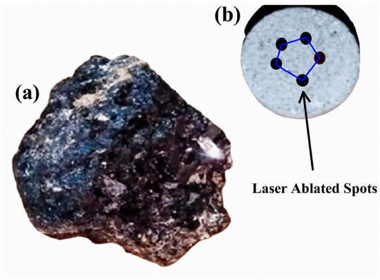
Figure 1.
(a) The rare earth geological raw sample from Gilgit-Baltistan, Pakistan and (b) pellet of the rare earth sample showing laser-ablated spots.
2.2. LIBS System
For the LIBS-based qualitative analysis, we used a Q-switched Nd:YAG laser (Brilliant B, Quantel), 100 mJ pulse energy at 532 nm, 5 ns pulse duration, and 10 Hz repetition rate [27,28,29]. The time-integrated LIBS experiments were performed at a 2 μs time delay between the laser pulse and the opening of the detection system, and a 1 ms integration time. A quartz lens of 20 cm focal length was used to focus the laser beam on the sample’s surface for ablation and plasma formation in the air at atmospheric pressure. The diameter of the focused laser beam on the sample surface was determined by employing the following formula [30]:
where d represents the diameter of the focused laser beam, λ denotes the laser wavelength (532 nm), f corresponds to the focal length of the lens (20 cm), and D signifies the diameter of the laser beam incident on the focusing lens surface (6 mm). The resulting diameter of the focused spot was approximately 43 μm. The time-integrated LIBS experiments were conducted using a laser pulse energy of approximately 100 mJ. This specific laser energy was chosen after optimizing the signal-to-noise ratio of the observed spectrum. The sample was placed on a rotary stage to expose a fresh surface for every laser shot. The surface inhomogeneity and statistical errors were minimized by recording the average spectrum of at least ten laser shots. A collecting lens, along with an optical fiber, was placed near the pellet’s surface to record the laser-produced plasma plume emission. A set of six miniature spectrometers (Avantes, Apeldoorn, Netherlands), each equipped with 10 μm wide slits, and 3648 pixel CCDs, was used to register the time-integrated emission spectra covering the wavelength range from 220 nm to 970 nm. The input to all the six spectrometers was provided through a bunch of six optic fibers, combined in a common unit coupled with a collecting lens at the end. Each of the six spectrometers captures spectra within distinct wavelength ranges: the first spectrometer covers the region from 220 nm to 339 nm, the second from 338 nm to 440 nm, the third from 439 nm to 576 nm, the fourth from 575 nm to 688 nm, the fifth from 687 nm to 777 nm, and the sixth from 776 nm to 961 nm. A complete spectrum was made by combining these spectra using an Excel sheet and the Origin software for further analysis. The response curves of these spectrometers differ, as they depend on the quantum efficiency of the grating and the detector in each spectrometer. The intensities of the spectrometers were factory-calibrated using the standard technique, such as using a Deuterium lamp. The instrumental resolution of our system is (0.06 ± 0.01) nm at 600 nm [31].
2.3. LA-TOF-MS Experimental Setup
A locally fabricated two-meter linear laser ablation time-of-flight mass spectrometer (LA-TOF-MS), comprising a stainless-steel chamber of 30 cm diameter and flight tube, was used to determine the elemental concentration. The stainless-steel chamber contains an ionization region and three extraction electrodes (). Two of the three extraction electrodes had 1 cm openings at the center, covered with a fine tungsten mesh. A turbo-molecular pump was used to maintain the vacuum at mbar during the experiment. A 500 MHz digital storage oscilloscope (Tektronix), coupled with a personal computer, was used to record and analyze the ion signals. The specifics of this system have been outlined in our previous papers [29,30,31,32]. In LA-TOF-MS, a 532 nm laser beam of about 5 mJ was focused on the sample target surface, with a lens of 70 cm focal length, producing fluence of about 20 J/cm2 that ablated the sample and produced ions of the constituent elements.
2.4. EDX Analysis
Furthermore, EDX is a rapid technique that is highly suitable for analyzing minerals containing REEs and determining their distribution within a complex matrix. It is particularly beneficial for geological samples with low concentrations of REEs. In this study, the REE sample was subjected to EDX analysis using a scanning electron microscope (SEM) equipped with an EDX system. X-ray emissions emitted from the sample’s surface were detected using a 30 mm2 Si (Li) detector. The chemical composition of all constituent elements in the REE sample was determined using Oxford-Instruments X-MaxN-20 EDX instruments, which were connected to the SEM and operated at 20 keV.
3. Results and Discussion
3.1. LIBS Emission Studies
We adopted a fast procedure for the qualitative elements analysis of the REE samples acquired from a specific area of Pakistan. In the first step, we recorded the LIBS spectra of all the pure rare earth oxides, and an atlas of the spectra was prepared as a reference. In the next step, the spectra of the unknown samples were recorded under identical experimental conditions. In the third step, the qualitative analysis was performed by comparing the spectrum of the sample under investigation with that of the REE spectra and locating the common lines. This procedure helped us to pinpoint the presence of REEs in the sample within a very short time. Figure 2 shows the emission spectra of the sample along with that of REOs (La, Ce, Nd), and Ti recorded using laser pulse energy covering the wavelength region from 250 nm to 750 nm.
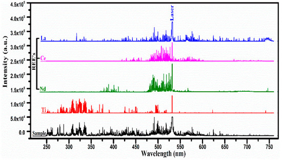
Figure 2.
The optical emission spectra of the laser-produced plasma on the surface of the rare earth sample and pure rare earth oxides (REO); La2O3, CeO2, Nd2O3, and Ti covering the wavelength range from 250 nm to 750 nm.
The stacking layers of five different spectra for the rare earth sample, along with the spectra of pure (rare earth oxides), lanthanum (La2O3) cerium (CeO2), neodymium (Nd2O3), and titanium, show several common lines at specific wavelengths belonging to different elements. The strongest line at 532 nm is the second harmonic of the Nd:YAG laser which also serves as an internal reference for comparison of the spectra. Interestingly, very rich line structures are evident between 475 nm and 530 nm in La, Ce, Nd, and the sample, whereas a rich line structure is observed between 300 nm and 350 nm in the spectrum of the sample as well as in the spectrum of titanium. In the spectrum of the sample, the neutral (I) and singly ionized (II) spectral lines of Si, Mg, Ca, and Ti have been identified, along with that of La, Ce, and Nd, confirming the presence of these elements in the sample. The molecular spectra of their oxides have not been identified in the LIBS spectra that might appear if the spectra are recorded at a longer delay time. The spectra were recorded with different laser energies. The signal intensities increase as the laser energy is increased. We optimized the laser energy so that signal-to-noise ratio is improved.
The spectral lines of each element in the sample have been identified with the help of the NIST database [33]. Moreover, in the present study, the experiments were conducted in air at atmospheric pressure. The Hα line was not detected in these spectra as we dried the sample in an oven for more than 10 h to remove moisture. The identified spectral lines, along with their wavelengths, are presented in Table 1. To elaborate on the persistent lines of Ti, La, Ce, and Nd in the spectra of the rare earth sample, we present different sections of the spectra in Figure 3, Figure 4, Figure 5, Figure 6 and Figure 7.

Table 1.
The main spectral lines of neutral (I) and singly ionized (II) elements used for the analysis of the rare earth samples [33].
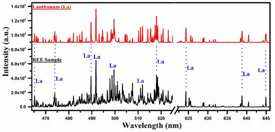
Figure 3.
A comparison of the laser-induced plasma spectra of the REE sample with that of lanthanum oxide (La2O3) covering the wavelength range from 465 nm to 645 nm.
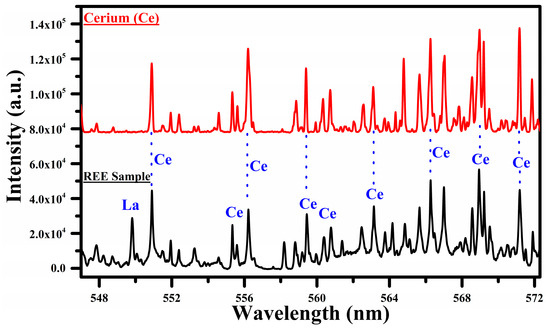
Figure 4.
A comparison of the spectra of the rare earth sample with that of cerium oxide (CeO2) covering the wavelength range from 547 nm to 572 nm.
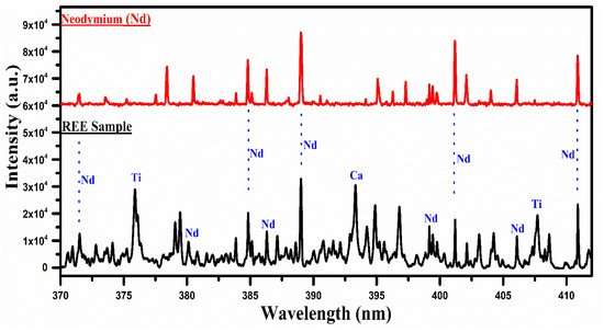
Figure 5.
A comparison of the spectra of the rare earth sample with that of neodymium oxide (Nd2O3) covering the wavelength range from 370 nm to 415 nm.
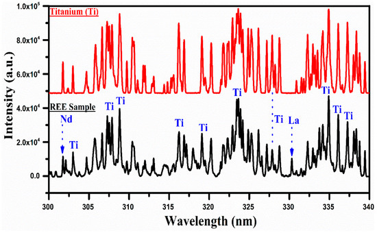
Figure 6.
A comparison of the spectra of the rare earth sample with that of titanium covering the wavelength range from 300 nm to 340 nm.
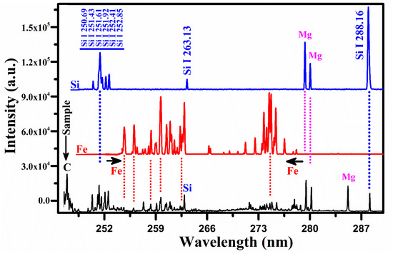
Figure 7.
A comparison of the spectrum of the rare earth sample with that of the silicon and iron covering the wavelength range from 246 nm to 290 nm.
In Figure 3, a comparison of the spectra of La with the REE sample covering the wavelength region from 465 nm to 645 nm is presented. It shows many overlapping characteristic spectral lines in the spectrum of lanthanum, and that of the sample marked by the blue dotted lines, signifying that the elements contained in the two samples are the same. In this wavelength region, the neutral, as well as the singly ionized lines of lanthanum, are identified. The central emission lines of La at 489.99, 492.18, 465.03, 470.26, 510.62, 514.54, 515.87, 517.73, 521.19, 523.96, 624.99, 628.86, and 629.63 nm have been detected in the sample by comparing the wavelengths listed in the NIST database [33]. The region between 622 nm and 647 nm displays only the spectral lines of La in both spectra, confirming the presence of lanthanum in the sample.
In Figure 4, we show a comparison between the spectra of Ce and the sample covering the wavelength region 547 nm to 572 nm. In this region, the main emission lines of Ce I at 544.92, 556.60, 559.59, 560.13, 567.78, 569.29, 569.70, 571.90, 577.31, 578.82, 581.29, and 594.09 nm have been identified. The common lines in the spectra of cerium and the sample are marked with blue dotted lines, showing that most of the lines belong to Ce. The spectral lines of Ce observed in this experiment are enlisted in Table 1. Interestingly, a strong emission line of La I at 550.13 nm is also observed in this selected region, which reveals the presence of La in the sample. Certainly, in Figure 2, the most interesting region for the cerium (Ce) is from 470 to 570 nm. We observed a rich spectrum of cerium (Ce) with that of lanthanum (La) and neodymium (Nd) from 470 nm to 570 nm. The emission lines at 471 nm, 479 nm, 482 nm, 500 nm, 504 nm, 518 nm, 524 nm, 527 nm, 535 nm, 546 nm, 551 nm, 556 nm, 566 nm, and 569 nm coincide in the wavelength region from 470 nm to 570 nm. We have reproduced the spectral region from 547 nm to 572 nm because of the minimum interference of the cerium (Ce) lines with that of lanthanum (La), as shown in Figure 4.
In Figure 5, the spectrum of the REE sample is compared with that of neodymium oxide, covering the spectral range from 370 nm to 415 nm. Several lines are common between the two spectra, particularly around 385 nm, 389 nm, 401 nm, and 411 nm, and are marked in blue color, which qualitatively establishes the presence of Nd in the sample. It is, however, worthwhile to mention that the strong emission lines of Ti I at 376.34 nm and Ca II at 393.37 nm are also present in this spectral region. Although the most interesting region for neodymium (Nd) is from 470 nm to 570 nm, as shown in Figure 2, this region contains several lines of the neodymium (Nd) that overlap with that of the La and Ce. For instance, the lines at 470 nm, 479 nm, 482 nm, 485 nm, 488 nm, 489 nm, 492 nm, 521 nm, 524 nm, 527 nm, 529 nm, 530 nm, 535 nm, 548 nm, and 566 nm are observed overlapping with that of La and Ce lines. Therefore, we have presented the spectral region from 370 nm to 415 nm where Nd lines appear dominantly. The major emission lines of Nd I have been identified at 463.42, 488.38, 489.69, 492.45, 494.48, and 495.48 nm, and are presented in Table 1.
In Figure 6, the spectrum of titanium is compared with that of the REE sample in the wavelength region from 300 nm to 340 nm. The spectra show a few bunches of well-separated structures around 307 nm, 317 nm, 324 nm, and 335 nm. There is a good correspondence between the spectrum of Ti and that of the REE sample. There is hardly any line of any other element in this selected wavelength region of the spectrum except a couple of weak lines of Nd II at 301.84 nm and La II at 330.31 nm. Thus, the presence of titanium in the sample is qualitatively established based on the comparison of the LIBS spectra of Ti and that of the REE sample recorded under identical experimental conditions. The emission lines of Ti I have been observed at 319.19 nm, 319.99 nm, 320.38 nm, and 321.79 nm, and Ti II at 301.72, 302.37, and 302.97 nm. Furthermore, we have identified and included the different emission lines of Si and Fe within the wavelength range of 246 nm to 290 nm. These lines, along with those of Ti, La, Ce, and Nd, were observed and are presented in Table 1.
Figure 7 shows a comparison of the emission spectrum of the sample with that of the silicon (Si) and iron (Fe). The common lines between the spectrum of Si and that of the sample are represented by the dotted lines in blue color. The group of silicon lines around 251 nm belongs to silicon. A comparison with the iron spectrum also reveals common lines between the two spectra. There are two well-separated structures of Fe between 254 and 262 nm and between 271 and 277 nm, two lines of singly ionized Mg at 279.55 nm and 280.27 nm along, with its resonance line at 285.21 nm, and the carbon line at 247.85 nm. Thus, the presence of C, Fe, Si, and Mg in the rare earth sample is validated unambiguously. Having identified the spectral lines of all the elements present in the sample, our next task was to determine the plasma parameters for the quantitative analysis.
3.2. Plasma Characterization
To characterize the laser-produced plasma based on optical emission studies, certain conditions are to be satisfied, i.e., the plasma is optically thin and follows the local thermodynamic equilibrium (LTE) condition. We used the line intensity ratio method to validate the condition of an optically thin plasma [34,35]. We used the emission lines that had nearly the same energies as, or very close energies to, the upper levels to minimize the temperature dependence. The intensity ratios of the experimentally observed spectral lines and the values calculated from the spectroscopic parameters are in good agreement with a 5% error. For illustration, the experimentally calculated intensity ratio using La I at transitions 514.54 nm and 517.73 nm is 0.65, whereas the intensity ratio calculated from the spectroscopic parameters is 0.67. The error relative to the theoretical ratio is less than 3% which is acceptable. Thus, the plasma can be considered as satisfying the optically thin condition.
Having established that the plasma is optically thin, the excitation temperature was calculated using the Boltzmann plot method. The spectroscopic parameters of the optically thin emission lines of La I, Ce I, and Nd II used to draw the Boltzmann plots were obtained from the NIST database [31]. The spectroscopic parameters of the persistent lines including wavelength (nm), upper-level energy (eV), transition, statistical weight, and transition probability (s−1) are presented in Table 2. To draw the Boltzmann plots, these lines were carefully chosen as they lie in a narrow spectral region, where the efficiency of the detector remains nearly constant, that reduces the errors associated with the line intensity measurements. The excitation temperatures were calculated using the Boltzmann plot method, considering several spectral lines and their relative line intensities [35,36,37,38]:
Table 2.
Spectroscopic parameters of the emission lines of La I, Ce I, and Nd II used to draw the Boltzmann plots [33].
Here, is the intensity of the spectral line due to the k→i transition, is the spectral wavelength, h is the Planks constant, c is the speed of light, is the transition probability, is the statistical weight of the upper level, is the energy of the upper level, is the Boltzmann constant, Te is the excitation temperature, N is the total number density, and is the partition function. A plot of the left-hand side of this equation versus the energies of the upper levels yields a straight line and its slope is equal to . The Boltzmann plots corresponding to the La I, Ce I, and Nd II lines are shown in Figure 8, displaying good linearity; the linear correlation coefficients are , , and . The excitation temperatures were determined from the slopes of the lines corresponding to La I, Ce I, and Nd II as 10,000 ± 500 K, 9000 ± 500 K, and 10,500 ± 500 K respectively.
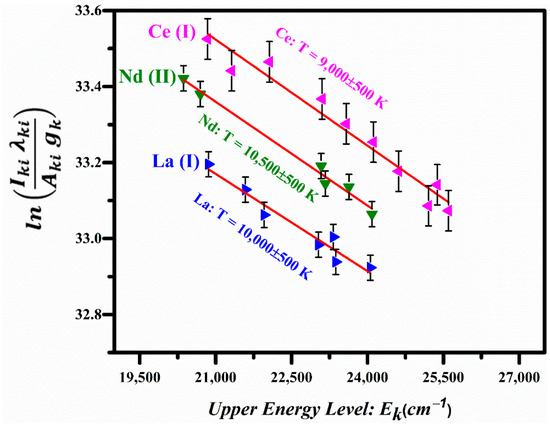
Figure 8.
Boltzmann plots based on the emission lines of La I, Ce I, and Nd II.
The electron number density, was calculated from the full width at half maximum (FWHM) of the Stark-broadened line profile of the singly ionized titanium (Ti II) at 368.62 nm [34,39]:
Here, represents the full width at half maximum, denotes the Stark broadening parameter (0.0154 nm) specific to the Ti II line being considered, and Nr indicates the reference number density, which is for the singly ionized line. A Voigt fitting profile of the Ti II line at 368.62 nm, which takes into account the instrumental resolution and the Doppler width [40], is reproduced in Figure 9. The calculated value for the is .
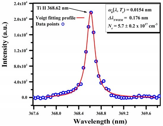
Figure 9.
A typical Stark-broadened line profile of Ti II at 368.62 nm, along with the Voigt fitting profile.
According to McWhirter’s criterion, the collisional mechanisms should dominate the radiative processes for a stationary and homogeneous plasma to be in local thermodynamic equilibrium (LTE). McWhirter proposed a lower limit for the to satisfy the LTE condition, which is as follows [41]:
Here, is the energy difference between the upper and lower electron volt (eV) levels and is the excitation temperature in kelvin (K). The electron number density is calculated using this relation for an elevated and ΔE = 2.40 eV as Ne = . This value of the number density is much lower than that of ( determined from the Stark-broadened line profile Ti II line at 368.62 nm. Thus, the plasma can be considered close to the LTE condition. Once it is established that the plasma is optically thin and in LTE, the plasma parameters have been used to estimate the elemental concentration using the CF-LIBS technique.
3.3. Compositional Analysis Using LIBS, LA-TOF-MS, and EDX
In the LIBS-based quantitative analysis, the calibration-free laser-induced breakdown spectroscopy (CF-LIBS) technique has been used to determine the elemental composition as described in several research articles [42,43,44,45,46]. In brief, to determine the concentration of the neutral atoms, the Boltzmann equation is used [43]:
Here, factor F, which considers the efficiency of the collection system and the volume of the plasma, is an experimental parameter. F can be determined by normalizing the concentrations of the elements found in the sample, is the concentration of the neutral atom, is the integrated line intensity of the k→i transition, is the statistical weight of the upper level, ) is the transition probability, Ek (eV) is the energy of the upper level, is the thermal energy of the plasma in eV, and kB is the Boltzmann constant. The partition function is dependent on temperature and can be calculated using the following relation:
Here, the symbol represents the statistical weight, denotes the energy of the upper level, and the term represents the thermal energy of the plasma. All the spectroscopic parameters used for the compositional analysis were taken from the NIST database [33]. The calculated value of electron density and the average value of the plasma temperature is used for the analysis. The concentration of the neutral atoms in the sample is calculated using Equation (5).
However, to calculate the concentration of the ionized species, the Saha–Boltzmann equation was used [17,43,44,45,46]:
Here, is the thermal energy of the plasma in eV, is the ionization energy of the element α, is the electron number density, is the concentration of the γ + 1 charge state, and and are the partition functions of the upper charge state (γ + 1) and lower charge state (γ), respectively. The contribution of any element present in the sample is the sum of the neutral and ionic contributions [17]:
The concentration (Wt.%) of each constituent in the sample was calculated using Equation (9). To validate the LIBS results, the elemental analysis was also performed using a locally constructed two-meter linear laser ablation time-of-flight mass spectrometer (LA-TOF-MS) [30,32,46]. The mass spectrum of the rare earth sample obtained by LA-TOF-MS is shown in Figure 10. The spectrum shows the ion signals corresponding to all the constituent elements, C, Na, Mg, Si, Ca, Fe, and Ti together with the rare earth elements, La, Ce, and Nd. The peak height of each element reflects its concentration, which was determined from the area under the curve analysis. Silicon is the dominant element followed by titanium and iron. A contour around 35 μs has been observed that corresponds to all the rare earth elements present in the sample, lanthanum, cerium, and neodymium. As lanthanum has no isotopes, but Ce possesses four isotopes and neodymium has five isotopes, therefore, their signals became merged and formed a broad contour. To extract the compositions of these elements, a deconvolution procedure of the overlapping peaks was performed using commercially available software (Origin 2023). A linear regression calibration graph between the time-of-flight (T) and the square root of the mass () is presented as an inset (b) in Figure 10 and exhibits a strong correlation, with .
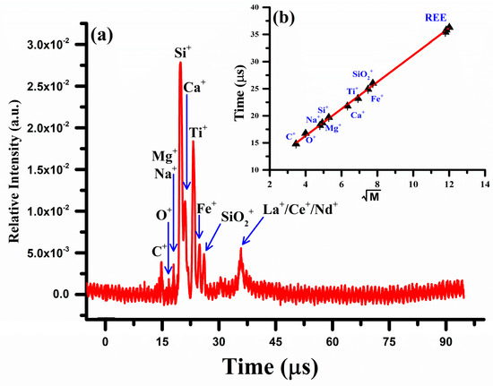
Figure 10.
(a) Laser ablation time-of-flight mass spectrum of the REE sample (b) A linear regression calibration connecting the time of flight (T) and the square root of the mass.
To further supplement our studies, the EDX spectrum of the rare earth sample was also acquired using the EDX analytical technique. Figure 11 shows a characteristic X-ray spectrum of the sample. The electron scanning area of the sample is displayed as an inset (b) in this figure. The data reveal that Si is present as the major element (Kα peak at 1.739 keV) along with C (0.277 keV), O (0.525 keV), Na (1.04 keV), Mg (1.25 keV), Ca (3.69 keV), Ti (4.51 keV), and Fe (6.40 keV). The bunch of peaks around 4–6 keV corresponds to the Lα lines of the REE; La (4.65 keV), Ce (4.84 keV), and Nd (5.23 keV) and Lγ lines; La (5.788 keV), and Ce (6.052 keV). It is worth mentioning that the Kα line of titanium lies at 4.511 keV which is superposed with the Lα line of lanthanum (4.6 keV). The resolution of the equipment is not sufficient enough to resolve these two peaks. However, the Kα and Kβ lines of iron at 6.4 keV and 7.06 keV, respectively, are well resolved. The contribution from the elements such as C and O is evident in the figure. A comparison between the EDX spectrum and that of LIBS shows that all the elements detected by LIBS are also observed by EDX. However, the EDX spectrum shows well-resolved peaks corresponding to lanthanum, cerium, and neodymium that were merged in the LA-TOFMS spectrum. This is because, in EDX, we obtain peaks at different energies (keV) corresponding to the Lα and Lγ lines of these elements whereas in LA-TOFMS we observe peaks corresponding to the arrival time (μs) of the ions at the detector. Both techniques provide supplementary results and confirm the presence of the REE in the sample we have analyzed.
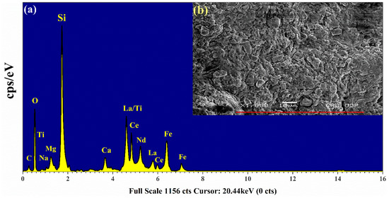
Figure 11.
(a) Energy-dispersive X-ray analysis (EDX) spectrum of rare earth sample (b) The microphotograph displays a specific scanned area of the pellet’s surface.
The elements which were identified in the rare earth sample, along with their concentrations detected with CF-LIBS, LA-TOF-MS, and EDX, are presented in Table 3. The standard deviation (SD) of the concentration (Wt.%) obtained through the CF-LIBS technique was calculated using the following equation [47,48,49]:
Table 3.
A comparison of LIBS results with LA-TOF-MS and EDX, including relative accuracy and standard deviation at 2 μs delay time, for different elements detected in the rare earth sample.
Here, σ is the standard deviation (SD), is the value from each data, is the mean value of the data, and n indicates the number of values or size of the sample. The calculated relative standard deviation for LIBS measurements is within 10 rel.%. To enable simple comparison, the relative accuracy (R.A) is calculated using the following formula:
Here, Nx represents the expected value of N for the xth measurement, while Ny represents the measured value of N for the yth measurement. The calculated (R.A) was determined to be within the range of 0.01–0.14. To conduct a comparative study, the elemental concentration (Wt.%) of the rare earth sample was determined using the LA-TOF-MS and EDX techniques. The results are presented in Table 3 for comparison. In LA-TOF-MS, the area under the curve was used to calculate the composition of each element present in the sample as La = 9.04 Wt.%, Ce = 11.77 Wt.%, and Nd = 8.09 Wt.%. The concentration extracted using LA-TOF-MS was in good agreement with the quantitative results obtained using the CF-LIBS technique. In the EDX analysis, the same REEs (La, Ce, and Nd) were detected as the major elements in the sample. For example, the concentration of REEs was La = 9.39 Wt.%, Ce = 10.66 Wt.%, and Nd = 9.08 Wt.%, which is in good agreement with that obtained using CF-LIBS and LA-TOF-MS.
Moreover, in LIBS measurements, the elements C and O pose challenges for the determination of their chemical composition due to the volatilization of carbonates and water. When a laser is used to generate plasma on the sample surface, the high temperatures cause the release of carbon dioxide (CO2), from carbonates, and water vapor (H2O), from hydrated ores or moisture present in the target sample. This volatilization process leads to the loss of carbon and oxygen atoms from the sample, affecting the accuracy of the chemical composition evaluation. The volatilization of CO2 and H2O creates uncertainties in the LIBS measurements because it changes the original chemical composition of the sample. The loss of C and O can lead to inaccurate elemental ratios, particularly for C and O themselves, as well as for other elements whose concentrations are affected by the presence of carbonates or water. To address this problem, researchers in LIBS analysis often employ various correction techniques. These techniques aim to account for the volatilization effects and adjust the measured elemental ratios accordingly. The corrections may involve calibrations based on reference samples with known compositions, or the application of mathematical models to compensate for the volatilization-induced deviations.
Consequently, in this work involving CF-LIBS calculations, the weight percentages of C and O appear relatively low, even though they are present in ores as oxides with higher weight percentages. This discrepancy arises from the normalization process, where the total weight percentage of all elements is adjusted to 100 Wt.%. As a result, the weight percentages of C and O may be significantly lower in LIBS calculations compared to their actual weight percentages in the form of oxides found in ores. Therefore, the low appearance of C and O contents in CF-LIBS is a consequence of the weight percentage normalization process used to accurately represent the overall elemental composition of the sample.
The composition obtained from all three techniques, CF-LIBS, LA-TOF-MS, and EDX, are in agreement. The slight differences in the CF-LIBS compositions are attributed to factors such as line intensity measurements, transition probabilities, laser spot positions, and plasma constraints. In LA-TOF-MS, the major error occurs due to the deconvolution procedure, signal drift, and measured area through the peak fitting [50,51].
The main objective of the present study was to detect and quantify the REEs in the samples obtained from the Northern Areas of Pakistan. For the comparative analysis, we studied the rare earth samples using three analytical techniques, LIBS, LA-TOF-MS, and EDX. The EDX, coupled with a scanning electron microscope (SEM), is commonly employed for the qualitative analysis of raw materials and it has a detection limit of around along with a depth profile of approximately 5 microns (5 μ) [52,53]. The elements having concentrations of tenths of Wt.% to several Wt.%, such as C, Na, Mg, Si, Ca, Ti, and Fe, along with light REEs such as La, Ce, and Nd, were detected successfully by EDX. However, it is worth revealing that EDX is unable to detect very light elements, such as H, Li, Be, and B, due to its detection constraints. On the other hand, in LA-TOF-MS, there is no particular restriction on the size or dimension of the target sample. A few mJ of laser energy is used to ablate the sample surface and it has the potential to detect all the elements in the Periodic Table. The mass spectrum of LA-TOF-MS (see Figure 10) shows that all the elements detected by LIBS are detectable in the mass spectra except for Mg. Since the atomic mass of Na (22.989769 Daμ) and Mg (24.305 Da) are very close in comparison to the other elements, this explains why their ionic peaks are nearly overlapping, and the signal height also becomes modified due to the low concentration of Na and Mg in the sample. The Na and Mg signal lies precisely on the calibration line according to the relation. The present study establishes that an efficient way to detect different elements present in various samples is through comparing their LIBS spectra recorded under identical experimental conditions. The LIBS results show a good detection limit from C to Nd in the rare earth geological sample that is in good agreement with that of LA-TOF-MS for the elements such as C, O, Na, Mg, Si, Ca, Ti, Fe, La, Ce, and Nd.
3.4. Limit of Detection of the Analyzed Rare Earths
To determine the limit of detection (LOD) for the REEs, several target samples of powdered metal oxides were prepared using La, Ce, and Nd from Sigma–Aldrich. A base or substrate metal of powdered zinc (99.99% pure) was utilized, onto which different concentrations (ppm) of rare earth metal oxides, including La2O3, CeO2, and Nd2O3, were doped. We used zinc powder of high purity as a matrix as it was available in our laboratory and, secondly, the emission spectrum of zinc contains a very limited number of spectral lines, at 636.22, 481.05, 472.22, 468.21, and at 330.26 nm; the overlapping of the lines with those of the sample spectrum is also not obvious. The concentration of each rare earth metal in the five different samples is presented in Table 4.
Table 4.
The concentration (ppm) of each REE in various samples of zinc matrix.
The five as-prepared samples, with zinc as a base metal, were utilized to calculate the limit of detection of rare earth metals. All five zinc-matrix-based samples were studied by LIBS through optimized experimental conditions, 532 nm laser wavelength, 100 mJ pulse energy, 1 ms integration time, and 2 μs delay time. Various emission lines of rare earth metals having ~107 s−1 transition probability, minimal interference effects, and being free from self-absorption and non-resonance, along with the zinc emission line, were selected to draw the calibration curves as shown in Table 5.
Table 5.
Emission lines of rare earth metals used for the estimation of LOD.
The characteristic spectral lines such as La (I) at 521.2 nm, Ce (II) at 551.2 nm, Nd (II) at 410.9 nm, and Zn (I) at 481.1 nm were selected in the present analysis. The zinc emission line is used to normalize the signal amplitude of the La, Ce, and Nd lines by taking the fraction of the signal amplitude of the corresponding line to the signal amplitude of the Zn (I) emission line at 481.1 nm. In the LIBS spectrum of the five prepared zinc-matrix-based samples, the Zn emission lines were found to be free from interference and self-absorption. The calibration curves of the elements La, Ce, and Nd present in the zinc matrix showed good linear fitting, as shown in Figure 12a–c, within the experimental error.
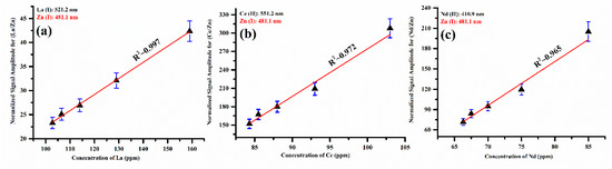
Figure 12.
The normalized calibration curves illustrate the signal amplitude of Zn (I) at 481.1 nm, displaying the signal amplitude ratio (a) of (La/Zn) with La, (b) of (Ce/Zn) with Ce, and (c) of (Nd/Zn) with Nd.
The LOD of the zinc matrix was calculated using the following relation [54]:
Here, σ indicates the standard deviation of the background signal and b reveals the calibration sensitivity (slope of the calibration curve). Table 6 presents the calculated limit of LOD, reported LOD, and relative standard deviation (RSD %) for the rare earth metals La, Ce, and Nd. The RSD is determined by multiplying the standard deviation (SD) by 100 and dividing the result by the average value.
Table 6.
The limit of detection (LOD) values of La, Ce, and Nd along with the R2 and RSD (%).
The LOD values for the elements La, Ce, and Nd, obtained using the calibration curve laser-induced breakdown spectroscopy (CC-LIBS) technique, align well with the reported values by Yang et al. [55]. Yang et al. utilized surface-enhanced laser-induced breakdown spectroscopy to detect rare earth elements (La, Ce, Pr, and Nd) in an aqueous solution. Therefore, LIBS has established itself as an advanced analytical technique, in combination with LA-TOF-MS and EDX, for assessing rare earth elements (REEs) in both standard and raw materials. Nevertheless, several experimental factors, including the intensity of the analytical signal, the signal-to-noise ratio, the sample surface homogeneity, the elemental concentration, and the reproducibility of LIBS analytical results, can influence the LOD in LIBS-based measurements.
4. Conclusions
Three analytical techniques, LIBS, LA-TOF-MS, and EDX, were used to analyze and quantify the REEs in geological ore samples obtained from the Northern Areas of Pakistan. The qualitative identification of the spectral lines of La, Ce, and Nd in the LIBS spectra confirmed the presence of these elements in the samples. Moreover, the spectral lines of Si, Ti, Na, Mg, Ca, and Fe in the LIBS spectra confirmed their presence in the sample. The excitation plasma temperature (Te) and electron number density (Ne) were calculated to perform a quantitative analysis of the constituent elements. The procedure of first recording the LIBS spectra of all the REEs under the same experimental conditions and making an atlas of the spectra, then comparing them with the spectrum of any unknown sample, provided an efficient detection methodology for the presence of REEs. To demonstrate the capabilities of LIBS, a comprehensive compositional analysis of the rare earth elements was performed using different analytical techniques, including LA-TOF-MS and EDX. Interestingly, these alternative methods produced results that exhibited a favorable level of agreement with the results acquired through LIBS. In addition, the LOD values of the La, Ce, and Nd elements, acquired via calibration curve laser-induced breakdown spectroscopy (CC-LIBS), were found to be in good agreement with the values reported for LIBS in the literature. The comparative study suggests that LIBS can be used as a potential technique for the detection of rare earth elements in geological ores. The information acquired from this study will generate further interest for scientists to extract and separate these REEs from this ore found in the Northern Areas of Pakistan.
Author Contributions
Conceptualization, Methodology, Investigation, validation, Conceptualization, Writing—original draft, A.F.; Formal analysis, Investigation, R.A. (Raheel Ali); Resources, Formal analysis, Data curation, Funding acquisition, M.W.; Formal analysis, Investigation, U.L.; Investigation, Methodology, R.A. (Rizwan Ahmad); Visualization, Formal analysis, Investigation, Z.A.U.; Conceptualization, Methodology, Writing—review & editing, M.A.B. All authors have read and agreed to the published version of the manuscript.
Funding
This manuscript received no external funding.
Data Availability Statement
The data presented in this study are available on request from the corresponding author.
Acknowledgments
We are grateful to the Pakistan Academy of Sciences and the National Canter for Physics for the financial support to establish this facility for LIBS and LA-TOF-MS studies. In addition, the authors would like to express their gratitude to the Department of Mining and Geological Engineering at The University of Arizona for generously providing financial support for the current study.
Conflicts of Interest
The authors declare that they have no known competing economic interests or personal relationships that could have appeared to affect the work described in this paper.
References
- Noack, C.W.; Jain, J.C.; Stegmeier, J.; Hakala, J.A.; Karamalidis, A.K. Rare Earth Element Geochemistry of Outcrop and Core Samples from the Marcellus Shale. Geochem. Trans. 2015, 16, 6. [Google Scholar] [CrossRef] [PubMed]
- Gaft, M.; Nagli, L.; Gornushkin, I.; Raichlin, Y. Review on Recent Advances in Analytical Applications of Molecular Emission and Modelling. Spectrochim. Acta Part B At. Spectrosc. 2020, 173, 105989. [Google Scholar] [CrossRef]
- Gaft, M.; Raichlin, Y.; Pelascini, F.; Panzer, G.; Ros, V.M. Imaging Rare-Earth Elements in Minerals by Laser-Induced Plasma Spectroscopy: Molecular Emission and Plasma-Induced Luminescence. Spectrochim. Acta Part B At. Spectrosc. 2019, 151, 12–19. [Google Scholar] [CrossRef]
- Bhatt, C.R.; Jain, J.C.; Goueguel, C.L.; McIntyre, D.L.; Singh, J.P. Determination of Rare Earth Elements in Geological Samples Using Laser-Induced Breakdown Spectroscopy (LIBS). Appl. Spectrosc. 2018, 72, 114–121. [Google Scholar] [CrossRef] [PubMed]
- Reinhardt, N.; Proenza, J.A.; Villanova-de-Benavent, C.; Aiglsperger, T.; Bover-Arnal, T.; Torró, L.; Salas, R.; Dziggel, A. Geochemistry and Mineralogy of Rare Earth Elements (REE) in Bauxitic Ores of the Catalan Coastal Range, NE Spain. Minerals 2018, 8, 562. [Google Scholar] [CrossRef]
- Lefticariu, L.; Klitzing, K.L.; Kolker, A. Rare Earth Elements and Yttrium (REY) in Coal Mine Drainage from the Illinois Basin, USA. Int. J. Coal Geol. 2020, 217, 103327. [Google Scholar] [CrossRef]
- Cotton, S. Lanthanides and Actinides; Red Globe Press: London, UK; Macmillan Education Ltd.: London, UK, 1991. [Google Scholar]
- Moeller, T. The Chemistry of the Lanthanides; Pergamon Texts in Inorganic Chemistry; Elsevier: Amsterdam, The Netherlands, 2013; Volume 26. [Google Scholar]
- Zawisza, B.; Pytlakowska, K.; Feist, B.; Polowniak, M.; Kita, A.; Sitko, R. Determination of Rare Earth Elements by Spectroscopic Techniques: A Review. J. Anal. At. Spectrom 2011, 26, 2373–2390. [Google Scholar] [CrossRef]
- Orihashi, Y.; Hirata, T. Rapid Quantitative Analysis of Y and REE Abundances in XRF Glass Bead for Selected GSJ Reference Rock Standards Using Nd-YAG 266 nm UV Laser Ablation ICP-MS. Geochem. J. 2003, 37, 401–412. [Google Scholar] [CrossRef]
- Fedorowich, J.S.; Richards, J.P.; Jain, J.C.; Kerrich, R.; Fan, J. A Rapid Method for REE and Trace-Element Analysis Using Laser Sampling ICP-MS on Direct Fusion Whole-Rock Glasses. Chem. Geol. 1993, 106, 229–249. [Google Scholar] [CrossRef]
- Zhang, Y.; Zhang, T.; Li, H. Application of Laser-Induced Breakdown Spectroscopy (LIBS) in Environmental Monitoring. Spectrochim. Acta Part B At. Spectrosc. 2021, 181, 106218. [Google Scholar] [CrossRef]
- Sdvizhenskii, P.A.; Lednev, V.N.; Grishin, M.Y.; Pershin, S.M. Deep Ablation and LIBS Depth Elemental Profiling by Combining Nano- and Microsecond Laser Pulses. Spectrochim. Acta Part B At. Spectrosc. 2021, 177, 106054. [Google Scholar] [CrossRef]
- Cremers, D.A.; Radziemski, L.J.; Loree, T.R. Spectrochemical Analysis of Liquids Using the Laser Spark. Appl. Spectrosc. 1984, 38, 721–729. [Google Scholar] [CrossRef]
- St-Onge, L.; Kwong, E.; Sabsabi, M.; Vadas, E.B. Rapid Analysis of Liquid Formulations Containing Sodium Chloride Using Laser-Induced Breakdown Spectroscopy. J. Pharm. Biomed. Anal. 2004, 36, 277–284. [Google Scholar] [CrossRef]
- Miziolek, A.W.; Palleschi, V.; Schechter, I. (Eds.) Laser Induced Breakdown Spectroscopy; Cambridge University Press: Cambridge, UK, 2006. [Google Scholar]
- Ciucci, A.; Corsi, M.; Palleschi, V.; Rastelli, S.; Salvetti, A.; Tognoni, E. New Procedure for Quantitative Elemental Analysis by Laser-Induced Plasma Spectroscopy. Appl. Spectrosc. 1999, 53, 960–964. [Google Scholar] [CrossRef]
- Fortes, F.J.; Moros, J.; Lucena, P.; Cabalín, L.M.; Laserna, J.J. Laser-Induced Breakdown Spectroscopy. Anal. Chem. 2013, 85, 640–669. [Google Scholar] [CrossRef]
- Gaudiuso, R.; Dell’Aglio, M.; De Pascale, O.; Loperfido, S.; Mangone, A.; De Giacomo, A. Laser-Induced Breakdown Spectroscopy of Archaeological Findings with Calibration-Free Inverse Method: Comparison with Classical Laser-Induced Breakdown Spectroscopy and Conventional Techniques. Anal. Chim. Acta 2014, 813, 15–24. [Google Scholar] [CrossRef] [PubMed]
- Abedin, K.M.; Haider, A.F.M.Y.; Rony, M.A.; Khan, Z.H. Identification of Multiple Rare Earths and Associated Elements in Raw Monazite Sands by Laser-Induced Breakdown Spectroscopy. Opt. Laser Technol. 2011, 43, 45–49. [Google Scholar] [CrossRef]
- Phuoc, T.X.; Wang, P.; McIntyre, D. Detection of Rare Earth Elements in Powder River Basin Sub-Bituminous Coal Ash Using Laser-Induced Breakdown Spectroscopy (LIBS). Fuel 2016, 163, 129–132. [Google Scholar] [CrossRef]
- Bhatt, C.R.; Yueh, F.Y.; Singh, J.P. Univariate and Multivariate Analyses of Rare Earth Elements by Laser-Induced Breakdown Spectroscopy. Appl. Opt. 2017, 56, 2280–2287. [Google Scholar] [CrossRef]
- Castro, J.P.; Babos, D.V.; Pereira-Filho, E.R. Calibration Strategies for the Direct Determination of Rare Earth Elements in Hard Disk Magnets Using Laser-Induced Breakdown Spectroscopy. Talanta 2020, 208, 120443. [Google Scholar] [CrossRef]
- Gaft, M.; Nagli, L.; Gorychev, A.; Raichlin, Y. Rare-Earth Elements Detection Using Diatomic Molecular Laser-Induced Plasma Spectroscopy. Spectrochim. Acta Part B 2022, 192, 106426. [Google Scholar] [CrossRef]
- Harikrishnan, S.; Ananthachar, A.; Choudhari, K.S.; George, S.D.; Chidangil, S.; Unnikrishnan, V.K. Laser-Induced Breakdown Spectroscopy (LIBS) for the Detection of Rare Earth Elements (REEs) in Meteorites. Minerals 2023, 13, 182. [Google Scholar] [CrossRef]
- Fayyaz, A.; Asghar, H.; Alshehri, A.M.; Alrebdi, T.A. LIBS Assisted PCA Analysis of Multiple Rare-Earth Elements (La, Ce, Nd, Sm, and Yb) in Phosphorite Deposits. Heliyon 2023, 9, e13957. [Google Scholar] [CrossRef] [PubMed]
- Ahmed, R.; Ahmed, N.; Iqbal, J.; Baig, M.A. An Inexpensive Technique for the Time Resolved Laser Induced Plasma Spectroscopy. Phys. Plasmas 2016, 23, 083101. [Google Scholar] [CrossRef]
- Iqbal, J.; Mahmood, S.; Tufail, I.; Asghar, H.; Ahmed, R.; Baig, M.A. On the Use of Laser-Induced Breakdown Spectroscopy to Characterize the Naturally Existing Crystal in Pakistan and Its Optical Emission Spectrum. Spectrochim. Acta Part B 2015, 111, 80–86. [Google Scholar] [CrossRef]
- Umar, Z.A.; Ahmed, N.; Ahmed, R.; Liaqat, U.; Baig, M.A. Elemental Composition Analysis of Granite Rocks Using LIBS and LA-TOF-MS. Appl. Opt. 2018, 57, 4985–4991. [Google Scholar] [CrossRef]
- Fayyaz, A.; Liaqat, U.; Yaqoob, K.; Ahmed, R.; Umar, Z.A.; Baig, M.A. Combination of Laser-Induced Breakdown Spectroscopy and Time-of-Flight Mass Spectrometry for the Quantification of CoCrFeNiMo High Entropy Alloys. Spectrochim. Acta Part B 2022, 198, 106562. [Google Scholar] [CrossRef]
- Jabbar, A.; Akhtar, M.; Mehmood, S.; Ahmed, N.; Umar, Z.A.; Ahmed, R.; Baig, M.A. On the Detection of Heavy Elements in the Euphorbia indica Plant Using Laser-Induced Breakdown Spectroscopy and Laser Ablation Time-of-Flight Mass Spectrometry. J. Anal. At. Spectrom. 2019, 34, 954–962. [Google Scholar] [CrossRef]
- Ahmed, N.; Ahmed, R.; Umar, Z.A.; Baig, M.A. Laser Ionization Time-of-Flight Mass Spectrometer for Isotope Mass Detection and Elemental Analysis of Materials. Laser Phys. 2017, 27, 086001. [Google Scholar] [CrossRef]
- NIST Database. 2021. Available online: https://physics.nist.gov/PhysRefData/ASD/lines_form.html (accessed on 30 September 2022).
- Cremers, D.A.; Radziemski, L.J. Handbook of Laser-Induced Breakdown Spectroscopy; John Wiley & Sons: Hoboken, NJ, USA, 2013. [Google Scholar]
- Asghar, H.; Ali, R.; Baig, M.A. Determination of Transition Probabilities for the 3p → 3s Transition Array in Neon Using Laser Induced Breakdown Spectroscopy. Phys. Plasmas 2013, 20, 123302. [Google Scholar] [CrossRef]
- Zhang, S.; Wang, X.; He, M.; Jiang, Y.; Zhang, B.; Hang, W.; Huang, B. Laser-Induced Plasma Temperature. Spectrochim. Acta Part B 2014, 97, 13–33. [Google Scholar] [CrossRef]
- Zhang, P.; Liu, X.; Lin, M.; Zhang, J. Research on the Spatio-Temporal Characteristics of High Energy Pulsed Plasma Jets. Phys. Plasmas 2022, 29, 093505. [Google Scholar] [CrossRef]
- Aragón, C.; Aguilera, J.A. Characterization of Laser-Induced Plasmas by Optical Emission Spectroscopy: A Review of Experiments and Methods. Spectrochim. Acta Part B 2008, 63, 893–916. [Google Scholar] [CrossRef]
- Griem, H. Principles of Plasma Spectroscopy; Cambridge Monographs on Plasma Physics; Cambridge University Press: Cambridge, UK, 1997. [Google Scholar]
- Harilal, S.S.; Brumfield, B.E.; LaHaye, N.L.; Hartig, K.C.; Phillips, M.C. Optical Spectroscopy of Laser-Produced Plasmas for Standoff Isotopic Analysis. Appl. Phys. Rev. 2018, 5, 021301. [Google Scholar] [CrossRef]
- McWhirter, R.W.P. Chapter 5. Plasma Diagnostic Techniques; Academic Press: Cambridge, MA, USA, 1965. [Google Scholar]
- Drawin, H.W. Validity Conditions for Local Thermodynamic Equilibrium. Z. Für Phys. 1969, 228, 99–119. [Google Scholar] [CrossRef]
- David, W.; Hahn, R.; Nicolò, F. Laser-Induced Breakdown Spectroscopy (LIBS), Part II: Review of Instrumental and Methodological Approaches to Material Analysis and Applications to Different Fields. Appl. Spectrosc. 2012, 66, 347–419. [Google Scholar]
- Tognoni, E.; Cristoforetti, G.; Legnaioli, S.; Palleschi, V.; Salvetti, A.; Müller, M.; Panne, U.; Gornushkin, I.B. A Numerical Study of Expected Accuracy and Precision in Calibration-Free Laser-Induced Breakdown Spectroscopy in the Assumption of Ideal Analytical Plasma. Spectrochim. Acta Part B 2007, 62, 1287–1302. [Google Scholar] [CrossRef]
- Abbass, Q.; Ahmed, N.; Ahmed, R.; Baig, M.A. A Comparative Study of Calibration Free Methods for the Elemental Analysis by Laser Induced Breakdown Spectroscopy. Plasma Chem. Plasma Process. 2016, 36, 1287–1299. [Google Scholar] [CrossRef]
- Ahmad, N.; Ahmed, R.; Umar, Z.A.; Liaqat, U.; Manzoor, U.; Baig, M.A. Qualitative and Quantitative Analyses of Copper Ores Collected from Baluchistan, Pakistan Using LIBS and LA-TOF-MS. Appl. Phys. B 2018, 124, 160. [Google Scholar] [CrossRef]
- Mermet, J.M. Calibration in Atomic Spectrometry: A Tutorial Review Dealing with Quality Criteria, Weighting Procedures and Possible Curvatures. Spectrochim. Acta Part B 2010, 65, 509–523. [Google Scholar] [CrossRef]
- El Haddad, J.; Canioni, L.; Bousquet, B. Good Practices in LIBS Analysis: Review and Advices. Spectrochim. Acta Part B 2014, 101, 171–182. [Google Scholar] [CrossRef]
- Dai, Y.; Song, C.; Gao, X.; Chen, A.; Hao, Z.; Lin, J. Quantitative Determination of Al–Cu–Mg–Fe–Ni Aluminum Alloy Using Laser-Induced Breakdown Spectroscopy Combined with LASSO–LSSVM Regression. J. Anal. At. Spectrom. 2021, 36, 1634–1642. [Google Scholar] [CrossRef]
- Vardeman, S.B.; Wendelberger, J.R.; Wang, L. Calibration, Error Analysis, and Ongoing Measurement Process Monitoring for Mass Spectrometry. Qual. Eng. 2006, 18, 207–217. [Google Scholar] [CrossRef]
- Uerlings, R.; Matusch, A.; Weiskirchen, R. Standardization and Normalization of Data from Laser Ablation Inductively Coupled Plasma Mass Spectrometry. In Applications of Laser Ablation-Thin Film Deposition, Nanomaterial Synthesis and Surface Modification; Intech Publishing: London, UK, 2016; pp. 399–415. [Google Scholar]
- Kawai, J.; Ishii, H.; Matsui, Y.; Terada, Y.; Tanabe, T.; Uchiyama, I. Risk Assessment of TiO2 Photocatalyst by Individual Micrometer-Size Particle Analysis with On-Site Combination of SEM-EDX and SR-XANES Microscope. Spectrochim. Acta Part B 2007, 62, 677–681. [Google Scholar] [CrossRef]
- Aidene, S.; Semenov, V.; Kirsanov, D.; Kirsanov, D.; Panchuk, V. Assessment of the Physical Properties, and the Hydrogen, Carbon, and Oxygen Content in Plastics Using Energy-Dispersive X-ray Fluorescence Spectrometry. Spectrochim. Acta Part B 2020, 165, 105771. [Google Scholar] [CrossRef]
- Mohamed, W.T.Y. Improved LIBS limit of detection of Be, Mg, Si, Mn, Fe and Cu in aluminum alloy samples using a portable Echelle spectrometer with ICCD camera. Opt. Laser Technol. 2008, 40, 30–38. [Google Scholar] [CrossRef]
- Yang, X.; Hao, Z.; Yi, R.; Li, J.; Yu, H.; Guo, L.; Li, X.; Zeng, X.; Lu, Y. Simultaneous determination of La, Ce, Pr, and Nd elements in aqueous solution using surface-enhanced laser-induced breakdown spectroscopy. Talanta 2017, 163, 127–131. [Google Scholar] [CrossRef]


Disclaimer/Publisher’s Note: The statements, opinions and data contained in all publications are solely those of the individual author(s) and contributor(s) and not of MDPI and/or the editor(s). MDPI and/or the editor(s) disclaim responsibility for any injury to people or property resulting from any ideas, methods, instructions or products referred to in the content. |
© 2023 by the authors. Licensee MDPI, Basel, Switzerland. This article is an open access article distributed under the terms and conditions of the Creative Commons Attribution (CC BY) license (https://creativecommons.org/licenses/by/4.0/).