Experimental Uncertainty Analysis for the Particle Size Distribution for Better Understanding of Batch Grinding Process

Abstract

Uncertainty in industrial processes is very common, but it is particularly high in the grinding process (GP), due to the set of interacting operating/design parameters. This uncertainty can be evaluated in different ways, but, without a doubt, one of the most important parameters that characterise all GPs is the particle size distribution (PSD). However, is the PSD a good way to quantify the uncertainty in the milling process? This is the question we attempt to answer in this paper. To do so, we use 10 experimental grinding repetitions, 3 grinding times, and 14 Tyler meshes (more than 400 experimental results). The most relevant results were compared for the weight percentage for each size (WPES), cumulative weight undersize (CWU), or the use of particle size distribution models (PSDM), in terms of continuous changes in statistical parameters in WPES for different grinding times. The probability distribution was found to be changeable when reporting the results of WPES/CWU/PSDM, we detected the over-/under-estimation of uncertainty when using WPES/CWU, and variations in the relationships between sizes were observed when using WPES/CWU. Finally, our conclusion was that the way in which the data are analysed is not trivial, due to the possible deviations that may occur in the uncertainty process.

1. Introduction

In general, when we want to optimise a process, we need to know all of the information that characterises it, in order to propose possible solutions. At present, any process that needs to be optimised requires multiple sources of information, which present along with its characteristics. In this way, it becomes possible to define it, as well as to determine its components and behaviour under certain conditions. This allows for the proposal of possible solutions to the problem.

The way to optimise any process could be chosen from three major alternatives: (a) planning successive experimental trials, in which we take into consideration the used equipment, personnel, and time; (b) mathematical optimisation, where quality models are required, as well as algorithms and a good definition of the problem for analysis; and (c) hybrid system solutions utilising elements from the two previous alternatives, which could generate possibilities for the development of a benchmark, along with rigorous planning that allows us to extract the maximum knowledge and, finally, to develop a subsequent calculation method for its validation. The only disadvantage of this alternative is that it requires a multidisciplinary team for both the experimental and mathematical analyses.

Generally speaking, for any of the alternatives presented that we would consider adopting to develop any type of optimisation procedure, multiple challenges are presented, ranging from the proposal itself to the quality/quantity of the input data. This information can be obtained using rigorous operational protocols, different types of sensors, characterisation of analytical techniques, and analytical sample analysis techniques, to name just a few. These data allow the calculation process to be carried out, and, for this reason, the precision and accuracy of the information are important elements determining the final result. The need for high-quality data, which has been facilitated through technological development over the years, has also made it possible to detect the fluctuations (minimum and maximum limits) of the parameters being studied; therefore, from a statistical point of view, these fluctuations are known as uncertainty.

The formal definition of uncertainty is not unique, as it depends on the context, but some of the most-used definitions are as follows: Coleman and Steele (2018) described it as “the grade of goodness of a measurement, experimental result, or analytical (simulation) result” [1]; Schenck and Richardson (1979) described it as “what we think the error would be if we could and did measure it by calibration” [2] or, as the ISO/IEC guide 98 defined it, the “method of evaluation of uncertainty by statistical analysis of series of observations” [3]. These definitions establish the premise of the need for quality information, whether experimental or simulated, as it is possible to generate complete feedback in this way. With this, it becomes possible to improve the mathematical model used or the calculation methodology (e.g., improving operational limits or restrictions) [4]. The entire mathematical process of information analysis to quantify these fluctuations is known as uncertainty analysis (UA), where the phase in which feedback and re-evaluation are developed, in order to improve either the methodology or the model, is known as the verification and validation (V&V) phase [1].

The V&V phase consists of two complementary concepts that are used for continuous improvement, which Schwer, in 2005 [5], defined as follows: “verification is the assessment of the accuracy of the solution to a computational model by comparison with a known solution” and “validation is the assessment of the accuracy of a computational simulation by comparison with experimental data”.

These two concepts can be very difficult to apply, as they depend on the process that is being studied; for example, some processes have different phenomenological models that allow their reality to be accurately predicted. In this particular case, their parameters are well-defined, with known uncertainties. This can be achieved by means of high-quality sensors and very well-studied and validated experimental protocols. However, there are other processes whose phenomenology is very complex, either by their own mechanism or by the input parameters (e.g., high cross-interaction or high uncertainty, to name a few); therefore, their results could present differences with respect to reality. Nevertheless, if there is a possibility to execute the V&V phase, it could have relevant advantages, such as: (a) improving the understanding of the results, (b) providing credibility to the models used, (c) giving credibility to the simulation or optimisation performed, or (d) to propose protocols for continuous improvement in all phases of the calculation and experimentation carried out. In conclusion, there are processes that have epistemic and stochastic uncertainties, which are not easy to define or determine; many of these complexities can be found in the grinding process.

The grinding process aims to reduce particles, in order to obtain a required product size, as well as the best conditions for the flotation process; however, grinding equipment uses complex comminution mechanisms (i.e., different types of equipment may utilise compression, traction, impaction, shear, and/or attrition) [6,7] to reduce the size of the particles, which are common in the majority of standard equipment (e.g., ball mill, bar mill, pebble mill, autogenous grinding, and semi-autogenous grinding, to name a few).

To evaluate, model, simulate, and optimise this process, different investigations have been carried out, considering the likes of phenomenological models [8], population mass balance [9,10], and integrated research systems [11], all of which consider the concept of particle size distribution (PSD) as one of the most relevant indicators to represent the change in particle size.

PSD is a concept that was historically developed to determine the result of comminution, generally reported as a graph of the cumulative weight undersize (CWU) [5,6,11,12]. Actually, the PSD has always managed to be included in some way, and current studies have generated more complex systems which include population mass balance (PMB).

The PMB could be defined as: “population balance or mass size balance, that describes a family of modelling techniques that includes tracking and manipulating partially or complete particle size distribution as they proceed through the comminution process” [6]; with this, it is possible to subdivide into two groups, the first group being related to the characterisation of the comminution process, which has been widely studied and constantly updated, mainly in terms of its mathematical expressions [13,14,15,16]. Meanwhile, the second group uses it as an integrated system, including control systems, hybrid optimisation, and optimisation with uncertainty [8,9,17]. All of these investigations use input data, which can be quantified in different ways while trying to be as precise as possible. Among these parameters, we can observe feed material characterisation (e.g., mechanical strength, toughness, brittleness, and PSD), final product specifications (e.g., PSD, mineral liberation, energy, flow rates, and control size), and control parameters of the machines (e.g., energy, speed, sounds, and pressure) [7]. However, all of these advances have allowed for significant improvements to be made in the associated mathematical models and the evaluation of more complex systems through the use of new computational algorithms, better sensors, and new sample analysis equipment.

While the improvement of new sensors and equipment has allowed for improvement of the data, in terms of many of the parameters (mainly for the second group), updating of the experimental protocols to obtain the breakage rate constant (which allows for calculation of the PMB) has been relegated. The standard protocol using particle size control parameters (PSCP), including the areas $F_{80}$ and $P_{80}$, then obtains the evolution of the comminution process and allows for subsequent calculation of its coefficients; however, this form of analysis does not allow us to obtain all the possible interactions associated with the system under study.

Therefore, the question would be: does this affect, in any way, the information obtained from the PMB?

The answer to the question posed above, initially, is affirmative. This is foundational, as research generally relies on multiple elements that could be considered as “deviations” when detailing the traditional method for analysing the PSD. Therefore, this data may present unintended bias problems, which could generate over- or under-estimation of the final information (due to idealised analysis protocols). The next question to ask, in this context, is: what does this idealisation affect?

The answer would be, in general, the uncertainty and sensitivity analyses, due to the quality of the breakage rate constant, which would not allow us to obtain an adequate analysis of the PSD for its validation. The PSD analysis sequence is shown in Figure 1.

From Figure 1, it can be seen that: (a) it is possible to first define an “intrinsic uncertainty”, related to the variability of the results obtained from the grinding process; and (b) the results obtained are those generated by the different interactions between the minerals/balls/shells, under the effects of the designed conditions and type of equipment used, the properties and physical characteristics of the mineral, and the experimental protocol used.

The results of the weight percentage for each size (WPES) have a unique ID; therefore, they could show different types of distributions with different statistical parameters. However, they are produced under the same condition and, so, they are interdependent parameters. After this analysis, the “first uncertainty deviation” is presented and is associated with modification of the data from WPES to the PSD and particle size distribution model (PSDM). Finally, there is the “second uncertainty deviation”, where the PSCPs are determined from interpolations of the PSDM ($F_{80}$ or $P_{80}$) or other factors being used (e.g., reduction ratio or sorting coefficient).

Finally, based on all of these antecedents, it is possible to ask the following questions:

• Will the evaluation parameters that are used to quantify the PSD be sufficient?
• In a milling process, is it possible to detect possible sources of epistemic and stochastic uncertainties through a comprehensive particle size analysis?
• Will the uncertainty be the same for the parameters when they are evaluated in the form of WPES with respect to the CWU or when a PSDM is used?
• Considering the PSCPs that are selected to quantify the milling, how are they influenced by the uncertainty of the PSD?

Based on these questions, we sought to do the following in this work:

• Carry out an exhaustive analysis of data gathered from the PSD in order to obtain the most detailed uncertainty analysis.
• Identify potential faults/shortcomings of the traditional way of analysis/reporting on PSD results.
• Propose mathematical expressions that characterise the uncertainty of the PSD.

2. Methodology

As previously mentioned, the methodology for determining the UA can be developed in two ways (see Figure 2, which is based on the methodology of Schwer, 2005 [5]): the first is through experimentation, being an expensive alternative, due to the materials and time required. The second way is the simulation by means of random number generation techniques (this will not be carried out in the present work but is included in the Figure as an example to demonstrate that a complete methodology could involve an ideally integrated calculation process), with the main advantage of the lower input and time costs; however, the quality of the information obtained depends basically on the definition of the boundary conditions defined for the simulation process. Therefore, it is dependent on the heuristic knowledge of the scientist/engineer that develops the simulation/optimisation.

In the case of grinding, investigations have already been developed where it was simulated and optimised under the influence of uncertainty [12,17]. In general, it is worth asking whether, in the uncertainty data of the PSD, PSDM, or PSCP, the first or second deviation of the uncertainty is considered (as appropriate), or whether the uncertainties defined are adequate for the WPES (as it can generate the largest/smallest deviations between what is simulated/optimised and reality). Therefore, not much information has been reported, in terms of how they affect the uncertainty of the milling process, depending on how their data are analysed, making the V&V process lacking in comparison and determination of the model, adjustment technique, and objective function appropriate.

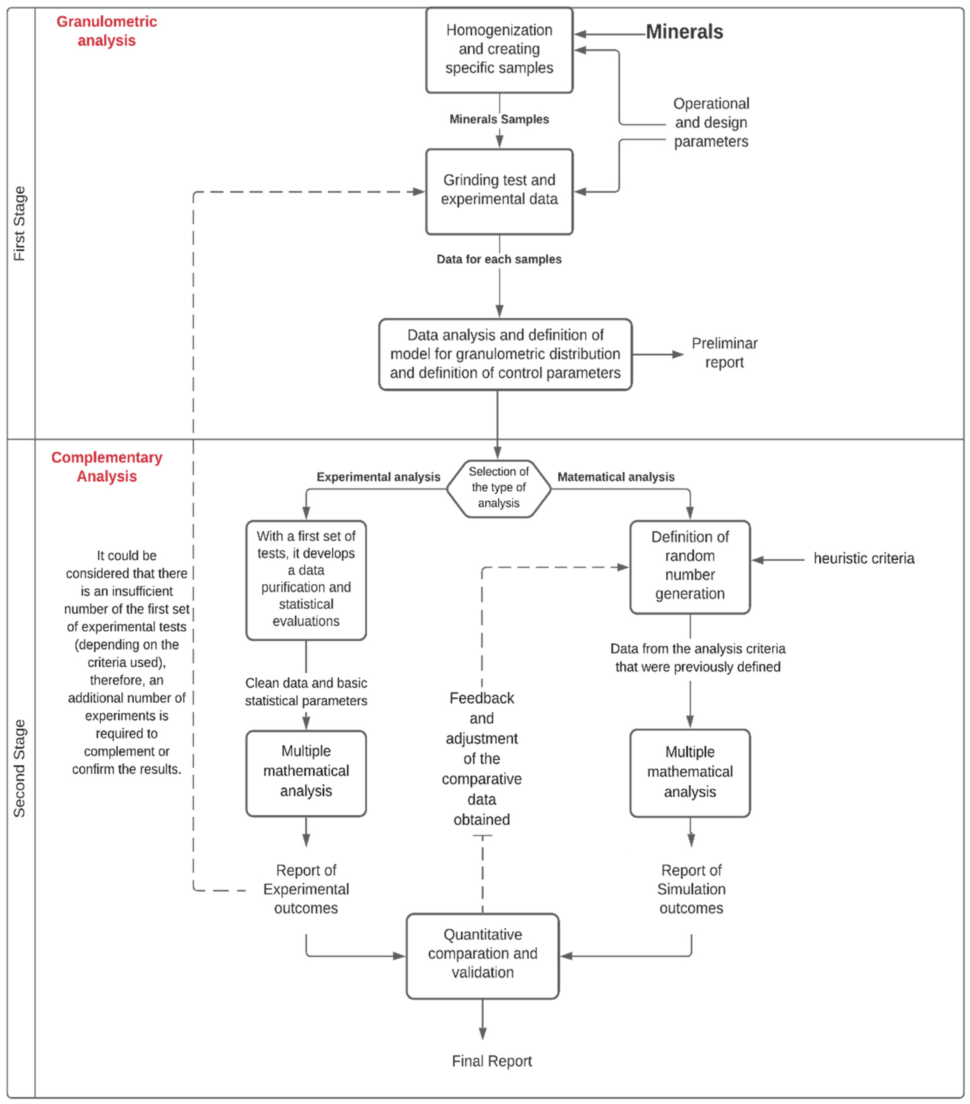
2.1. Proposed Methodology

The proposed methodology is divided into two chapters: the first is related to the granulometric analysis, while the second is related to the uncertainty analysis, as can be seen in Figure 2.

2.1.1. First Stage—Granulometric Analysis (GA)

At this point, the standard protocol was developed, similar to that used in any metallurgical laboratory using GA (i.e., an experimental protocol that allows us to obtain the data for analysis: WPES, PSD, PSDM, and PSCP); for example, homogenisation protocols, determination of physical characteristics, determination of chemical and mineralogical characteristics, the grinding parameters, filtering, and drying. The meshes to be used for the GA were defined, and, finally, the required data were reported. For this, we used the Rosin–Rammler model (RRM; Equation (1)), the Gates–Gaudin–Schumann model (GGS; Equation (2)), and least squares (Equation (3)):

$$F_{M\left(D\right)}=(1-exp(-{\left(\raisebox{1ex}{$D$}\!\left/ \!\raisebox{-1ex}{$m$}\right.\right)}^n\left)\right),$$

(1)

$$F_{M\left(D\right)}={\left(\raisebox{1ex}{$D$}\!\left/ \!\raisebox{-1ex}{$m$}\right.\right)}^n,$$

(2)

$$\epsilon ={\displaystyle \sum }_D{\left(F_{\left(D\right)}-F_{M\left(D\right)}\right)}^2,$$

(3)

where F_(D) is the PSD, $F_{M\left(D\right)}$ is the PSDM (RRM or GGS), $D$ is the particle size, $m$ is the size modulus, $n$ is the distribution modulus, and $\epsilon$ indicates the error, which is the quantity to be minimised.

2.1.2. Second Stage—Complementary Analysis

It was developed using the same experimental protocols that were used in the first stage, but a number of repetitions were included, allowing us to obtain enough statistical data and allowing for the development of multiple mathematical analyses to determine the UA, as explained below.

Descriptive statistical analysis [18,19]: Descriptive statistics are used to summarise data in a quantitative form from a collection of information. The main parameters are: Mean, median, mode, standard deviation, variance, kurtosis, and skewness, to mention a few. Graphics are also included, including histograms, box plots, and Q–Q plots.

Normality test analysis: A normality test is a statistical process used to determine whether a sample or any group of data fits a standard normal distribution. The normality test can be performed mathematically or graphically (i.e., parametric or non-parametric, respectively) [20,21]. There are multiple tests that allow for the evaluation of a group of data, such as D’Agostino’s K-squared test, the Jarque–Bera test, the Anderson–Darling test, the Kolmogorov–Smirnov test, and the Shapiro–Wilk test, to name a few [22]. The choice of test to use depends on multiple criteria; however, for this investigation, the Shapiro–Wilk test was chosen, as it is one of the most popular tests used when considering a small sample size.

The Shapiro–Wilk test [23] was created in 1965 and was originally restricted to a sample size less than 50. This test was the first test that was able to detect departures from normality due to either skewness, kurtosis, or both. It has become the preferred test, due to its good power properties. Given an ordered random sample $y_1<y_2<\cdots <y_n$, its expression is defined as:

$$W=\frac{{\left({{\displaystyle \sum }}_{i=1}^n{a}_i{y}_i\right)}^2}{{{\displaystyle \sum }}_{i=1}^n{\left(y_i-\overline{y_i}\right)}^2},$$

(4)

$$a_i=\left(a_1, \dots , a_n\right)=\frac{m^T{V}^{-1}}{{\left(m^T{V}^{-1}{V}^{-1}m\right)}^{\frac{1}{2}}},$$

(5)

where $y_i$ is the ith order statistic, $\overline{y}$ is the sample mean, $m={\left(m_1,\dots ,m_n\right)}^T$ are the expected values of the order statistics of independent and identically distributed random variables sampled from the standard normal distribution, and $V$ is the covariance matrix of those order statistics. The value of $W$ lies between zero and one. Small values of $W$ lead to the rejection of normality, whereas a value of one indicates the normality of the data.

Evaluation parameters: The parameters evaluated by different statistical techniques are diverse. We took into consideration the most important parameters reported [19], which could help to better elucidate the characteristics of the particles, in terms of not only milling but also flotation, thickening, and deposition in tailing dams [24,25,26]. For this reason, we reported the analysis of partial percentages retained, cumulative “sieving through particles”, and cumulative “sieving through adjusted particles” by PSDM. In this way, it was possible to quantify the trends for each of the results. In addition, the calculation of representative sizes, such as various parameters used in metallurgy, was included; however, other representative sizes also used in other areas of science (e.g., soil mechanics, geotechnics, and sedimentology) were also included, considering parameters such as $D_{75}$, $D_{60}$, $D_{30}$, $D_{25}$, and $D_{10}$. Finally, we also included expressions that allow for qualification of the process or the soils, such as the reduction ratio (Equation (6)), sorting coefficient (Equation (7)), coefficient of gradation (Equation (8)), and uniformity coefficient (Equation (9)). All of these parameters are very important, as they can serve as indicators of properties such as compressibility, shear strength, and hydraulic conductivity, among others.

$$RR=\raisebox{1ex}{$F_{80}$}\!\left/ \!\raisebox{-1ex}{$P_{80}$}\right.,$$

(6)

$$Sc=\sqrt[2]{\raisebox{1ex}{$D_{75}$}\!\left/ \!\raisebox{-1ex}{$D_{25}$}\right.},$$

(7)

$$Cc=\frac{D_{30}^2}{D_{60}{D}_{10}},$$

(8)

$$Uc=\raisebox{1ex}{$D_{60}$}\!\left/ \!\raisebox{-1ex}{$D_{10}$}\right..$$

(9)

Correlation analysis [18,25,27]: Correlation analysis is a statistical method used to evaluate the strength of the relationship between two quantitative variables (basic sensitivity analysis) [20]. A high correlation means that two or more variables have a strong relationship with each other, while a weak correlation means that the variables are hardly related. This technique is strictly connected to linear regression analysis, which is a statistical approach for modeling the association between a dependent variable (called the response) and one or more independent (or explanatory) variables. The correlation can be presented in a numeric (Pearson coefficient) or graphic (correlation matrix plot or scatter plot matrix) format. In the case of numeric or colour format, the correlation coefficient, r, varies between −1 and +1, where a perfect correlation is ±1, and 0 indicates the absence of correlations. Values of r between 0 and 1 reflect a partial correlation, which may be significant or not.

3. Results and Discussion

The case studies analysed below consider just one mineral, under different operational conditions.

3.1. Phase I: Granulometric Analysis

The mineral information is as follows: 182.5 kg of minerals; $F_{80}$ 1388 µm; specific gravity, 2.84; work index, 14.9 kWh/short ton. The mineral originated from a stratabound copper deposit and is hardly altered.

A geological analysis for the minerals was developed by a Motic SMZ-171 electronic magnifying glass (Motic, Hong Kong, China), an eyepiece 10×(Ø23)/magnification with a range of 0.75×–5×, which detects the presence of quartz, plagioclase, orthoclase, biotite, and muscovite, representing 98% of the samples, and the remaining 2% consists of chalcosine, bornite, molybdenite, chalcopyrite, and pyrite.

To obtain this information, we first performed a homogenisation process, based on laboratory protocols for the mining industry, in order to homogenise and create the samples to be evaluated in the mills and flotation.

Therefore, from ore, we generated 940 g samples. Multiple cycles were developed, in order to obtain completely homogenised materials, such that the effect of the variability of comminution was due to the grinding process itself.

The machines used for the first homogenisation step was a Rotary table splitter (DR-10, Labtech-HEBRO, Santiago, Chile), allowing for a division into six containers with a maximum capacity of 6 kg. The second homogenisation equipment was a prosplitter, allowing for division into 30 containers with a capacity of 300 gr. Both types of equipment utilised discharge hopper vibration and receptacle movement with variable speed.

General grinding protocol parameters were established, according to procedures reported by mining companies located in Chile. These parameters are described as the following: 138 iron balls of 1” diameter, with a total load weight of 10.220 kg, roller speed of 70 rpm, and a solid percentage of 67%. The grinding equipment used was a ball mill standardised with a laboratory scale, having a capacity of 5.2 L and a roller-HEBRO (variable RPM). The grinding process began by checking the size and weight of the steel balls, after which the load of the respective balls, the mineral, and, finally, the water was entered. The driving roller (HEBRO) was activated, after checking that the equipment was operating at 70 rpm and adjusting the timer control appropriately.

De-Sliming equipment was used for the removal of fine particles by wet sieving, using a 200 Ty mesh and a Labtech-HEBRO brand machine (Labtech-HEBRO, Renca, Chile). The products were then dried at 95 °C for 12 h. The GA was carried out in a Ro-tap W.S. Tyler (model RX-29-10) (W.S. Tyler, Mentor, OH, USA). The following meshes were used: #10, #20, #30, #40, #50, #60, #70, #100, #140, #200, #270, #325, and #−325 (all Tyler series). This option was used as it is the most widespread and economical technique for the realisation of GA.

Preliminary report: The results presented here are those obtained from the first grinding test, where PSD and PSDM were compared (Figure 3). In this case, the PSDM was evaluated using the RRM and GGS, and the choice of the best model was made through the use of least-squares minimisation (starting with the traditional adjustment technique and improving it through the use of a solver), being the one with the lowest error in the RRM (see Appendix A

Table A1. Adjustment results of the PSD and PSDM with least squares, for feed.

Size (µm)	PSD (%)	RRM (%)	ε	GGS (%)	ε
850–1700	100.00	100.00	0.00	100.00	0.00
600–850	46.58	44.73	3.43	33.99	0.25
425–600	33.50	35.06	2.44	26.27	0.88
300–425	25.34	27.04	2.92	20.36	0.20
250–300	19.91	20.51	0.36	15.73	3.02
212–250	17.47	17.67	0.04	13.75	4.19
150–212	15.80	15.41	0.15	12.17	0.48
106–150	12.87	11.49	1.89	9.42	1.40
90–106	10.61	8.51	4.38	7.29	1.34
74–90	8.45	7.38	1.14	6.46	0.00
63–74	6.39	6.21	0.03	5.59	1.01
53–63	4.58	4.62	0.00	4.37	0.37
43–53	3.76	3.84	0.01	3.74	13.99
35–43	0.00	0.00	0.00	3.21	10.32
0–35			16.79		37.44

,

Table A2. Adjustment results of the PSD and PSDM with least squares, for 4 min.

Size (µm)	PSD (%)	RRM (%)	ε	GGS (%)	ε
850–1700	100.00	97.36	6.96	100.00	0.00
600–850	79.50	80.44	0.88	83.98	19.99
425–600	67.39	69.21	3.32	67.04	0.12
300–425	56.28	57.78	2.26	54.05	4.98
250–300	46.03	45.97	0.00	42.82	10.29
212–250	41.78	40.49	1.66	38.06	13.85
150–212	37.94	35.66	5.23	34.00	15.51
106–150	30.23	27.52	7.35	27.35	8.24
90–106	22.94	20.75	4.81	21.85	1.18
74–90	20.01	18.09	3.71	19.66	0.12
63–74	15.99	15.48	0.26	17.47	2.19
53–63	9.60	13.31	13.80	15.61	36.15
43–53	8.06	11.44	11.47	13.96	34.84
35–43	5.53	9.90	19.15	12.56	49.46
0–35	0.0	0.00	0.00	0.00	0.00
sum			80.86		196.91

,

Table A3. Adjustment results of the PSD and PSDM with least squares, for 8 min.

Size (µm)	PSD (%)	RRM (%)	ε	GGS (%)	ε
850–1700	99.95	99.95	0.00	100.00	0.00
600–850	93.07	96.06	8.95	85.21	61.79
425–600	87.55	89.73	4.75	74.36	174.00
300–425	78.49	80.33	3.36	65.28	174.73
250–300	67.30	67.72	0.18	56.70	112.21
212–250	61.03	60.96	0.00	52.80	67.74
150–212	58.05	54.57	12.16	49.32	76.22
106–150	45.99	42.98	9.04	43.24	7.53
90–106	35.97	32.68	10.85	37.75	3.16
74–90	31.32	28.50	7.97	35.41	16.72
63–74	25.50	24.35	1.31	32.98	55.90
53–63	15.94	20.87	24.31	30.80	220.93
43–53	13.65	17.85	17.65	28.79	229.28
35–43	9.59	15.35	33.15	27.00	303.11
0–35	0.00	0.00	0.00	0.00	0.00
sum			133.70		1503.31

and

Table A4. Adjustment results of the PSD and PSDM with least squares, for 12 min.

Size (µm)	PSD (%)	RRM (%)	ε	GGS (%)	ε
850–1700	99.97	100.00	0.00	100.00	0.00
600–850	97.26	99.98	7.43	100.00	7.52
425–600	95.56	99.55	15.92	88.20	54.16
300–425	92.20	96.78	21.05	78.21	195.57
250–300	85.08	87.91	8.01	68.69	268.53
212–250	79.86	80.81	0.91	64.32	241.51
150–212	73.90	72.86	1.09	60.40	182.36
106–150	57.86	56.28	2.49	53.50	19.03
90–106	46.34	40.39	35.38	47.20	0.74
74–90	38.29	33.94	18.88	44.50	38.53
63–74	28.80	27.68	1.25	41.66	165.62
53–63	16.84	22.58	33.02	39.13	496.73
43–53	14.46	18.34	15.03	36.76	497.14
35–43	9.10	14.99	34.67	34.65	652.95
0–35	0	0	0	0	0
sum			195.14		2820.41

). In general, the evolution of the comminution in the mineral could be clearly noticed, showing its displacement to the fine zone of the PSD. The parameters $m$ and $n$ of RRM for the feed, as well as those after grinding for 4 min, 8 min, and 12 min, were 0.91 and 1.508, 0.93 and 503, 0.93 and 503, and 1.35 and 172.5, respectively.

With the respective trends obtained in Figure 3, it was possible to determine the PSCP of the feed and the grinding product, as presented in

Table 1. PSCP of the feed and under different grinding times.

PSCP	Feed Ore	4 min	8 min	12 min
$F_{80}$ (μm)	1388.4
$P_{80}$ (μm)	-	864	463	234
$D_{75}$ (μm)	1309.5	753	387	217
$F_{60}$ (μm)	1069.5	485	236	158
$D_{30}$ (μm)	523.6	149	87	77
$D_{25}$ (μm)	418.1	119	74	72
$D_{10}$ (μm)	101.6	64	46	46
RR	-	1.59	3	5.5
Sc	1.85	2.52	2.28	1.74
Cc	2.52	0.71	0.69	0.81
Uc	10.52	7.57	5.14	3.39

.

In general, the information obtained from both Figure 3 and Table 1 contain the basic parameters required to characterise and evaluate the milling/flotation process; for example, by determining $P_{80}$, it is possible to calculate the optimal milling times to obtain the best flotation conditions, as well as the determination of WI by means of different procedures.

Therefore, the first data report of this phase present this type of information. However, a question arises: is this is all the information that can be extracted from the GA?

3.2. Phase II: Complementary Analysis

In this stage, all kinds of techniques were included, in order to allow for the best analysis of the information of the PSD. In this case, the following techniques were used:

Data purification and statistical evaluation: As mentioned above, in this phase, ten repetitions of each of the tests were carried out. The results of the WPES, PSD, and RRM were compared under the grinding times indicated above; therefore, the analysis began with purification of the data, using a confidence range of 95% (

Table A5. Descriptive statistics of the 4 min test for the partial detainees with 95% confidence interval.

Size (µm)	Mean (%)	Median (%)	Standard Deviation (%)	Kurtosis	Skewness Coefficient
850–1700	20.27	20.18	0.45	2.73	1.49
600–850	12.30	12.22	0.34	7.17	2.58
425–600	11.88	12.10	0.52	−0.92	−0.20
300–425	9.64	9.75	1.14	6.01	2.19
250–300	4.21	4.21	0.04	1.63	0.04
212–250	3.65	3.57	0.12	0.35	1.03
150–212	7.56	7.62	0.50	0.07	0.02
106–150	7.55	7.54	0.32	0.08	0.59
90–106	3.27	3.21	0.34	1.49	0.38
74–90	4.30	4.37	0.47	0.01	0.39
63–74	6.25	6.25	0.18	0.88	0.49
53–63	1.23	1.22	0.20	0.25	0.24
43–53	2.75	2.83	0.22	1.63	0.32
35–43	5.06	4.99	0.36	1.12	0.34

,

Table A6. Descriptive statistics of the 8 min test for the partial detainees with 95% confidence interval.

Size (µm)	Mean (%)	Median (%)	Standard Deviation (%)	Kurtosis	Skewness Coefficient
850–1700	7.55	7.63	0.34	0.52	−0.91
600–850	5.49	5.51	0.04	−0.69	0.25
425–600	8.80	8.76	0.15	−0.63	0.63
300–425	10.68	10.66	0.24	1.94	1.28
250–300	5.62	5.59	0.26	6.18	2.29
212–250	4.76	5.01	0.69	6.89	−2.53
150–212	11.86	11.74	0.42	2.17	1.16
106–150	10.23	10.09	0.31	2.78	1.70
90–106	4.52	4.65	0.59	5.80	−2.15
74–90	5.99	5.94	0.33	0.75	0.11
63–74	9.28	9.18	0.58	2.21	1.32
53–63	2.06	2.01	0.21	−1.52	0.16
43–53	4.29	4.56	0.29	−0.96	0.20
35–43	8.81	8.68	0.43	−0.07	0.99

and

Table A7. Descriptive statistics of the 12 min test for the partial detainees with 95% confidence interval.

Size (µm)	Mean (%)	Median (%)	Standard Deviation (%)	Kurtosis	Skewness Coefficient
600–850	2.00	2.09	0.34	1.56	0.97
425–600	1.37	1.31	0.27	0.05	0.70
300–425	2.82	2.73	0.53	1.15	0.99
250–300	6.37	6.29	0.67	0.53	0.59
212–250	5.13	5.10	0.44	3.90	1.67
150–212	5.77	5.76	0.14	−0.54	−0.25
106–150	16.76	16.84	1.12	−0.33	0.03
90–106	11.69	11.63	0.84	3.20	0.36
74–90	8.11	8.05	0.62	−0.64	0.61
63–74	8.66	8.20	1.16	3.95	1.89
53–63	10.90	11.87	1.66	1.67	−1.42
43–53	3.29	3.44	0.51	−0.46	−0.75
35–43	6.01	6.05	0.52	−1.04	−0.04
0–35	11.09	11.31	1.64	1.70	0.99

). After that, a series of analyses were carried out, including the descriptive statistics of each of the results, a normality test, and, finally, a linear correlation analysis of the alternatives studied.

Uncertainty analysis with standard deviation: This analysis was possible thanks to the information provided by the descriptive statistics, using the standard deviation as an indicator. However, as mentioned previously, what we were looking for was to determine the most representative uncertainties of the grinding process. Therefore, it was considered that the WPES (reference value for analysis) provided quantification of the uncertainty with the smallest possible deviation.

As shown in Figure 4, the grinding time directly affected the magnitude and position of the media of WPES and its uncertainty, occurring in zones of influence with a breakpoint ($I_p$) of approximately 200 µm.

In general, in Figure 2, zones 1 and 3 show an orderly trend in the comminution process, while in zones 2 and 4, many trend changes and uncertainties can be seen. Finally, the 4 and 12 min grinding times were those for which the greatest uncertainties existed, having a maximum point at 300 µm for 4 min grinding, while 35 µm, 63 µm, and 150 µm were the maximum points for 12 min grinding. Meanwhile, for a grinding time of 8 min, a low uncertainty was observed for all sizes.

Another important element of Figure 4 (Up) is the trend of its WPES, where cleavage could be considered at times of 4 and 8 min as its possible main comminution mechanism, while, in 12 min, the mechanism was modified to abrasion.

On the other hand, when we compared the std. deviation, based on how the information is presented (WPES, PSD, and RRM), multiple fluctuations were observed (Figure 5). In some areas, the WPES were over-estimated (e.g., 600 µm, 250 µm, and 212 µm) while, in other areas, they were under-estimated (e.g., 300 µm and 35 µm), with respect to PSD and RRM. Therefore, there was a large fluctuation in the WPES, which was not reflected in the PSD or RRM, where it was considerably smoothed out.

The analysis of the 4 min milling case could not be extrapolated to the 8 min (Figure A1) and 12 min (Figure A2) cases. In the case of 8 min of grinding, the WPES in practically all sizes presented a sub-estimate with respect to PSD and RRM; however, it should be noted that the value of the standard deviation at 8 min was the lowest of the three cases. Finally, for the case of 12 min grinding (Figure A2), the same effect of sub-estimation of the uncertainty was seen as in the case of 8 min grinding, between the WPES vs. PSD and RRM. It must be clarified that they may possibly have a different calculation basis, due to the theory of the propagation of the error or that of the uncertainty [1], which is also explained in Figure 1.

Now, as seen in Figure 5 (Figure A1 and Figure A2), there was a difference between the standard deviation of the PSD and the RRM. This difference can be the cause in the phase of mathematical optimisation, by minimizing the least squares between the value of the PSD and RRM. This is due to the mathematical basis of the model used; the basis of the RRM was the Weibull distribution.

From Figure 6, it can be seen that this type of distribution was not clearly observed after a period of 4 min grinding, while after a period between 8 and 12 min, it could be considered as a Weibull distribution, up to approximately 200 µm, where the inflection point is located (being the same range as in Figure 4). This was also possible to see when determining the coefficients of the RRM model, using the linearisation of the semi-logarithmic graphs of data, by changing the slope. When this condition was taken into consideration, the PSD fits a bimodal distribution [26,28,29,30], rather than a unimodal distribution [6,31,32], in many cases.

This was justified as, in studies of the PSDM [32], the reference size for the PSD is considered in some cases, with the aim of developing complementary calculations (e.g., the work index), or the ideal form of the data distribution [6,28,29,30,31,32,33,34,35,36]. For an unknown reason, information regarding small sizes was not detected. Historically, several cases have been reported where the WPES trends did not have a defined pattern [36].

Another way to analyse this type of PSD without adjusting a binomial distribution is by evaluating it as unimodal distribution in two parts [25]. The possible mathematical expression is detailed in Equation (10). This option can also be substituted by different types of PSDM, due to the possibility that trends that might occur (for this case, the Rosin–Rammler bimodal model was used). Finally, this tendency is specific; for example, when the same type of mineral was processed with different operating protocols (Figure A3), the results could differ from those obtained in Figure 6. On the other hand, it was possible to evaluate another mineral (276.5 kg of material; 875 μm; specific gravity, 2.78; working index, 11.6 kWh/short ton). This mineral was from a copper porphyry deposit and significantly altered, but the same operating protocol was used. Again, the results (Figure A4) showed a completely different trend from those obtained in Figure 6; however, it should be mentioned that, in the results shown in Figure A4, Figure A5 and Figure A6, only duplicates were made and the uncertainty analysis information is not available.

$$F_{M\left(D\right)}=\{\begin{array}{c}\left(1-exp\left(-{\left(\raisebox{1ex}{$D$}\!\left/ \!\raisebox{-1ex}{$m_1$}\right.\right)}^{n_1}\right)\right)\begin{array}{cc}& \ge I_C\end{array}\\ \left(1-exp\left(-{\left({\raisebox{1ex}{$D$}\!\left/ \!\raisebox{-1ex}{$m$}\right.}_2\right)}^{n_2}\right)\right)\begin{array}{cc}& <I_C\end{array}\end{array}$$

(10)

Now, it is well-known that the use of PSDM generates a disturbance with respect to the PSD. Therefore, a question arises: How important could this be, quantitatively? For this, the normalised results of the quadratic errors are presented (Figure 6). In this way, it can be observed that the area presenting coarse sizes (850–210 µm) was the group that had the best adjustments, but, between 210 and 75 µm, the quality of the adjustment depended on the grinding time evaluated. Under 75 µm, all cases had the lowest quality adjustments, due to the tendency shown in Figure 4.

Finally, comparing the results of the mean, median, asymmetry coefficient, and kurtosis (Table A5, Table A6 and Table A7) for each of the sizes evaluated, our conclusion was that the mean and median did not have a very significant change. In the case of kurtosis, it was highly positive but without an excessively high value; therefore, it could be considered that the majority presented a leptokurtic curve. While the coefficient of skewness, in many cases had positive displacement, but they were still “small” values. Therefore, based on the fact that there was a very specific concentration of information, the normality analysis was developed.

The normality test analysis was conducted through the use of the Shapiro–Wilk test. In the first instance, it was evaluated for the WPES, confirming that most of the cases followed a normal distribution. Subsequently, the normality tests for the PSD and the data when the RRM was used were carried out, which showed that they also followed a normal trend, but, in some cases, information distortion was detected. Some cases where the analysis was distorted were in the range of 300–210 µm at 4 min of residence time and 850 µm at 8 min of residence, where, at 300–210 µm under 4 min, it changed from non-normal (WPES) to normal (PSD), then changed again to non-normal (RRM) (

Table A11. Descriptive statistics for ore a under 4 min grinding for descriptive parameters of PSD.

Item	Mean	Median	Standard Deviation	Kurtosis	Skewness Coefficient
$P_{80}$ (µm)	864.12	859.21	16.86	2.77	1.51
$D_{75}$ (µm)	750.02	724.85	10.37	4.05	1.82
$D_{60}$ (µm)	491.81	488.72	11.50	5.45	2.22
$D_{30}$ (µm)	147.59	149.00	2.85	−0.80	0.67
$D_{25}$ (µm)	118.21	118.25	2.66	−0.33	0.25
$D_{10}$ (µm)	65.16	65.53	1.19	−0.89	0.31
Rr	1.61	1.62	0.03	2.46	−1.42
Sc	2.52	2.52	0.02	0.39	−0.24
Cc	0.68	0.67	0.03	1.08	−0.73
Uc	7.55	7.57	0.20	−0.11	0.74

,

Table A12. Descriptive statistics for ore a under 8 min grinding for descriptive parameters of PSD.

Size	Mean	Median	Standard Deviation	Kurtosis	Skewness Coefficient
$P_{80}$ (µm)	463.63	464.00	5.025	−0.97	−0.19
$D_{75}$ (µm)	389.53	389.34	2.03	5.51	2.23
$D_{60}$ (µm)	234.54	234.04	2.03	5.51	2.23
$D_{30}$ (µm)	88.95	89.45	1.55	−0.71	−0.38
$D_{25}$ (µm)	76.15	76.17	1.44	−1.45	0.11
$D_{10}$ (µm)	47.41	47.72	0.82	0.44	−1.25
Rr	2.99	2.99	0.03	−0.95	0.22
Sc	2.26	2.27	0.02	−1.28	−0.42
Cc	0.71	0.71	0.02	0.45	−0.14
Uc	4.95	4.91	0.09	−0.15	0.97

and

Table A13. Descriptive statistics for ore a under 12 min grinding for descriptive parameters of PSD.

Size	Mean	Median	Standard Deviation	Kurtosis	Skewness Coefficient
$P_{80}$ (µm)	234.04	230.83	14.28	−0.56	0.26
$D_{75}$ (µm)	204.75	203.68	8.26	−0.39	0.47
$D_{60}$ (µm)	150.99	154.06	6.71	−0.17	−0.86
$D_{30}$ (µm)	73.09	72.99	2.63	−0.57	0.13
$D_{25}$ (µm)	68.19	67.89	2.57	1.17	−0.88
$D_{10}$ (µm)	43.33	43.00	2.48	1.26	−0.79
Rr	5.95	6.02	0.36	−0.63	−0.04
Sc	1.73	1.73	0.04	0.92	−0.48
Cc	0.82	0.81	0.06	−0.49	0.13
Uc	3.49	3.56	0.22	1.88	−1.17

).

Statistical analysis of PSCP: For this analysis, it can be shown that the uncertainty was different for each of the sizes. Figure 7 shows those with the highest and lowest standard deviations under all milling times. In the case of PSCP (Figure 8), the uncertainties had variable results, as influenced by the type of PSCP and the grinding time, with the sorting coefficient being that with the lowest standard deviation. Therefore, the effect of uncertainty in each of these parameters was not the same; therefore, it was necessary to study the effects of these parameters, in order to fully reflect the fluctuations that need to be detected (Table A11, Table A12 and Table A13).

Therefore, the uncertainty associated with each size of the PSD can be defined as a combination of uncertainties, where there may be different normal distributions and different ranges of uncertainties. This has proved different when performed for WPES (Equation (11)) and PSD, PSDM (Equation (12)), being directly influenced by the characteristics of the material in question (compare the results shown in Figure 6 and Figure A4), as well as the operating conditions (compare the results shown in Figure 4, Figure A3 and Figure A6). Finally, the expressions are as follows:

$$X_{S,t}=X_{S,t}^{true}\pm {\beta }_{S, t}^1\pm {\beta }_{S, t}^2\pm {\beta }_{S, t}^3,$$

(11)

$$R_{S,t}=R_{S,t}^{true}\pm {\beta }_{S, t}^1\pm {\beta }_{S, t}^2\pm {\beta }_{S, t}^3\pm {\beta }_{S, t}^4\pm {\beta }_{S, t}^5,$$

(12)

where $X_{S,t}$ is the determined value of the WPES for size $s$ and time $t$, $X_{S,t}^{true}$ is the true data for a WPES for size $s$ and time $t$, $R_{S,t}$ is the determined value of the PSD/PSDM for size s and time $t$, $R_{S,t}^{true}$ is the true data for a PSD/PSDM for size $s$ and time $t$, ${\beta }_{S, t}^1$ is the uncertainty associated with small changes in the grinding time $t$, ${\beta }_{S, t}^2$ is the uncertainty associated with the uncertainty of the grinding mechanism between the combined interaction of balls/associated particles upon repetition of the grinding tests at time $t$, and ${\beta }_{S, t}^3$ is the uncertainty associated with operational errors. In the treatment of the sample, ${\beta }_{S, t}^4$ is the uncertainty associated with the modification of passing from the partial retentions to the accumulated retentions/passes and ${\beta }_{S, t}^5$ is the uncertainty associated with the use of a granulometric model and specific optimisation methodology.

Within the operational errors, it is possible to specify the mineral mass losses, which are mainly associated with the stripping phase, due to the splashing of water on the ore. It was also detected in the solid/liquid separation phase, where ore was present within the walls of the filters and colloids and were lost in the filtered water. Therefore, the percentage losses for 4, 8, and 12 min of grinding were 3.9 ± 1.4%, 4.2 ± 0.78%, and 4.8 ± 0.56%, respectively.

Correlation analysis: From this observation, our conclusion is that the grinding process is characterised by a loss of mass at the largest sizes as distributed to the smallest sizes; therefore, values with negative correlations (red colour) make sense and not positive correlations (unless secondary phenomena are responsible).

In Figure 8 (as in Figure A5 and Figure A6), the element that can be highlighted is the modification of detectable correlations between the different sizes for the WPES and PSD. In addition, in Figure A5a, the correlations that were found could be at one point (430 µm, 300 µm, 250 µm), two points (90 µm and 63 µm), or, as in Figure A6a (106 µm), three points.

In addition, very slight correlations were also observed (close to white colour) or those with a value close to 0, which only occurred when there was a data cloud that filled the work area, producing a uniform distribution. Therefore, it was not possible to detect the main source contributing to the reduction in particle size.

Final report: At the end of all these analyses, it was possible to consider all the information previously presented, in order to determine a range of results for the WPES (

Table 2. PSCP of the feed under different grinding times.

Size (µm)	4 min			8 min			12 min
	Media (%)	Min. (%)	Max. (%)	Media (%)	Min. (%)	Max. (%)	Media (%)	Min. (%)	Max. (%)
600–850	20.34	19.90	21.37	7.61	6.92	8.03	2.04	1.57	2.80
430–600	12.31	12.12	12.92	5.50	5.44	5.57	1.37	1.03	1.87
300–430	11.88	11.11	12.66	8.80	8.64	9.05	2.82	2.19	3.90
250–300	9.64	6.81	10.89	10.69	10.43	11.20	6.37	5.51	7.60
210–250	4.21	4.15	4.26	5.62	5.38	6.26	5.13	4.68	6.15
150–210	3.64	3.52	3.84	4.76	2.98	5.24	5.77	5.55	5.96
106–150	7.56	6.79	8.40	11.86	11.33	12.77	16.76	14.98	18.61
90–106	7.55	7.13	8.12	10.23	10.01	10.93	11.70	10.16	13.41
75–90	3.27	2.18	4.50	4.51	3.04	5.12	8.11	7.32	9.14
63–75	4.30	3.45	5.01	5.99	5.42	6.56	8.67	7.48	11.37
53–63	6.25	5.94	6.46	9.28	8.70	10.54	10.86	7.28	12.17
45–53	1.23	0.86	1.54	2.06	1.77	2.35	3.30	2.37	3.80
35–45	2.74	2.43	2.99	4.29	3.86	4.72	6.01	5.26	6.70
0–35	5.06	4.54	5.60	8.81	8.35	9.59	11.09	9.10	14.55
Sum	100	90.93	108.58	100	92.25	107.94	100	84.48	118.03

) and, with this, to construct the PSD, PSDM, and PSCP, including all the observations that were obtained from the subsequent analyses.

4. Conclusions

Overall, we felt a need to remark on the following observations.

An extensive analysis of uncertainty was performed for WPES, PSD, PSDM, and PSCP data, showing that the uncertainty can be altered by the shape (probability distribution) and parameter (standard deviation) used to characterize the fine-grain distribution (granulometry).

It was also shown that a relevant part of the current problems inherent to concentration plants, pulp rheology control, and tailing deposition is the generation of fine size. As such, the traditional methodology for evaluating PSD and PSDM may not be sufficient to precisely detect such sizes (see Figure 5, where PSD and WPES have 0.35% v/s RRM with 0.25%; as well as Figure A2, where PSD has 1.5% v/s PSD and RRM has 1% of Std deviation). This is due, in part, to the underestimation of the models and/or the calculation methodology used by PSD and PSDM (presenting a smoothing/relaxed tendency).

A proposal was presented, in order to show how the uncertainty is decomposed within the particle size distribution, and that the traditional methodology is influenced by the concept of “propagation of uncertainty or propagation of error”, not necessarily only in the experimental process or during sampling, but also with respect to how the information is analysed and reported.

In general, all of the WPES results obtained were normally distributed but could be modified when used as PSD and PSDM (e.g., 250–300 µm for 4 min grinding time, 150–212 µm for 8 min grinding time, and 90–106 µm for 12 min grinding time), thus leading to alteration of the information.

The correlation analysis showed that there are certain coarser sizes that may be responsible for producing smaller sizes (e.g., 850 µm to 90 µm for 4 min grinding), presenting an inverse trend (p-value with negative value). There were also relationships that were not clear (p-value with a value close to zero), which may be due to the fact that the contribution to the size is related to several thicker sizes (e.g., 106 µm for 4 min grinding) while, on the other hand, there were cases in which there was a direct relationship (positive p-value), which has a mathematical, but not physical interpretation (e.g., 250 µm to 150 µm for 4 min grinding). Finally, when modifying the correlation analysis from WPES to PSD, these correlations were completely altered, which was seen in all of the cases studied; therefore, such alteration can be directly associated with the use of PSD.

We considered that it is necessary to determine the minimum number of samples necessary to carry out this type of research, as 10 repetitions may be insufficient. This is a requirement for all mathematical analyses; in particular, for normality tests and correlation analyses.

On the other hand, the best way to quantify the uncertainty in the PSD is still in doubt, as considering a mean, maximum, or weighted combination may not be enough. This can possibly be defined with respect to the requirements or needs of each mining company, engineer, or researcher. With this decision, it can become possible to apply the respective sensitivity analysis.

Finally, the methodology used in this work could be considered primitive, with respect to current sensors, computer systems, and analytical equipment, to name a few. However, it must always be considered that many metallurgical laboratories associated with production processes do not necessarily have the capacity to purchase up-to-date tools that allow for the detection of such problems, and, even if they did, the development of the V&V phase for this topic has been insufficient to date.

References

1. Coleman, H.W.; Steele, W.G. Experimentation, Validation, and Uncertainty Analysis for Engineers, 4th ed.; Wiley: Hoboken, NJ, USA, 2018; ISBN 9781119417989. [Google Scholar]
2. Schenck, H.; Richardson, P.D. Theories of engineering experimentation. J. Appl. Mech. ASME 1961, 28, 638. [Google Scholar] [CrossRef]
3. ISO—ISO/IEC Guide 98-3:2008—Uncertainty of Measurement—Part 3: Guide to the Expression of Uncertainty in Measurement (GUM: 1995). Available online: https://www.iso.org/standard/50461.html (accessed on 10 January 2021).
4. Kline, S.J. The purposes of uncertainty analysis. J. Fluids Eng. Trans. ASME 1985, 107, 153–160. [Google Scholar] [CrossRef]
5. Schwer, L.E. Verification and validation in computational solid mechanics and the ASME standards committee. WIT Trans. Built Environ. 2005, 84, 109–117. [Google Scholar]
6. Napier-Munn, T.; Wills, B.A. Wills’ Mineral Processing Technology; McGill University: Montréal, QC, Canada, 2005; ISBN 9780750644501. [Google Scholar]
7. Semsari, P.P.; Parian, M.; Rosenkranz, J. Breakage process of mineral processing comminution machines—An approach to liberation. Adv. Powder Technol. 2020, 31, 3669–3685. [Google Scholar] [CrossRef]
8. Taggart, A.F. Elements of Ore Dressing; John Wiles and Sons: New York, NY, USA, 1951. [Google Scholar]
9. Ramkrishna, D.; Singh, M.R. Population Balance Modeling: Current Status and Future Prospects. Annu. Rev. Chem. Biomol. Eng. 2014, 5, 123–146. [Google Scholar] [CrossRef] [Green Version]
10. Bilgili, E.; Scarlett, B. Population balance modeling of non-linear effects in milling processes. Powder Technol. 2005, 153, 59–71. [Google Scholar] [CrossRef]
11. Cisternas, L.A.; Lucay, F.A.; Botero, Y.L. Trends in modeling, design, and optimization of multiphase systems in minerals processing. Minerals 2020, 10, 22. [Google Scholar] [CrossRef] [Green Version]
12. Arancibia-Bravo, M.P.; Lucay, F.A.; López, J.; Cisternas, L.A. Modeling the effect of air flow, impeller speed, frother dosages, and salt concentrations on the bubbles size using response surface methodology. Miner. Eng. 2019, 132, 142–148. [Google Scholar] [CrossRef]
13. Gupta, V.K.; Sharma, S. Analysis of ball mill grinding operation using mill power specific kinetic parameters. Adv. Powder Technol. 2014, 25, 625–634. [Google Scholar] [CrossRef]
14. Hasan, M.; Palaniandy, S.; Hilden, M.; Powell, M. Simulating product size distribution of an industrial scale VertiMill® using a time-based population balance model. Miner. Eng. 2018, 127, 312–317. [Google Scholar] [CrossRef]
15. Herbst, J.A.; Fuerstenau, D.W. Scale-up procedure for continuous grinding mill design using population balance models. Int. J. Miner. Process. 1980, 7, 1–31. [Google Scholar] [CrossRef]
16. Powell, M.S.; Morrison, R.D. The future of comminution modelling. Int. J. Miner. Process. 2007, 84, 228–239. [Google Scholar] [CrossRef]
17. Sharma, S.; Pantula, P.D.; Miriyala, S.S.; Mitra, K. A novel data-driven sampling strategy for optimizing industrial grinding operation under uncertainty using chance constrained programming. Powder Technol. 2021, 377, 913–923. [Google Scholar] [CrossRef]
18. Brownlee, J. Machine Learning Mastery with R; Machine Learning Mastery: Melbourne, Australia, 2018. [Google Scholar]
19. Montgomery, D.C.; Runger, G.C.; Wiley, J. Applied Statistics and Probability for Engineers, 3rd ed.; John Wiley & Sons, Inc.: Hoboken, NJ, USA, 2003; ISBN 0471204544. [Google Scholar]
20. Saltelli, A.; Ratto, M.; Andres, T.; Campolongo, F.; Cariboni, J.; Gatelli, D.; Saisana, M.; Tarantola, S. Global Sensitivity Analysis: The Primer; John Wiley & Sons, Ltd.: Hoboken, NJ, USA, 2008; ISBN 9780470059975. [Google Scholar]
21. Siraj-Ud-Doulah, M. A Comparison among Twenty-Seven Normality Tests. Res. Rev. J. Stat. 2019, 8, 41–59. [Google Scholar]
22. Das, K.R.; Imon, A.H.M.R. A Brief Review of Tests for Normality. Am. J. Theor. Appl. Stat. 2017, 5, 2–12. [Google Scholar]
23. Razali, N.M.; Wah, Y.B. Power comparisons of Shapiro-Wilk, Kolmogorov-Smirnov, Lilliefors and Anderson-Darling tests. J. Stat. Model. Anal. 2011, 2, 21–33. [Google Scholar]
24. Das, B.M. Principles of Geotechnical Engineering; Cengage Le.: Stamford, CT, USA, 2010; ISBN 9780495411307. [Google Scholar]
25. Wills, B.; Napier-Munn, T. Mineral Processing Technology: An Introduction to the Practical Aspects of Ore Treatment and Mineral Recovery; Elsevier Science & Technology: Burlington, MA, USA, 2006; ISBN 0750644508. [Google Scholar]
26. Dallavalle, J.M. Micromeritics: The Technology of Fine Particles; Pitman Publishing Corporation: New York, NY, USA, 1943. [Google Scholar]
27. Gagné, F. Descriptive Statistics and Analysis in Biochemical Ecotoxicology. In Biochemical Ecotoxicology: Principles and Methods; Elsevier Inc.: Amsterdam, The Netherlands, 2014; pp. 209–229. [Google Scholar]
28. Dallavalle, J.M.; Orr, C.; Blocker, H.G. Fitting Bimodal Particle Size Distribution Curves. Ind. Eng. Chem. 1951, 43, 1377–1380. [Google Scholar] [CrossRef]
29. Brittain, H. Particle-size distribution, Part III: Determination by analytical sieving. Pharm. Technol. 2002, 26, 56–64. [Google Scholar]
30. Xu, Z.; Gautam, M.; Mehta, S. Cumulative frequency fit for particle size distribution. Appl. Occup. Environ. Hyg. 2002, 17, 538–542. [Google Scholar] [CrossRef] [PubMed]
31. King, R.P. Modeling and Simulation of Mineral Processing Systems; Elsevier Inc.: Amsterdam, The Netherlands, 2012; ISBN 0750648848. [Google Scholar]
32. Kelly, E.; Spottiswood, D. Introduction to Mineral Processing; John Wiley & Sons, Inc.: Hoboken, NJ, USA, 1982; ISBN 978-0471033790. [Google Scholar]
33. Kelsall, D.F.; Reid, K.J.; Restarick, C.J. Continuous Grinding in a Smallwet Ball Mill. Part III. A Study of Distribution of Residence Time. Power Technol. 1969, 3, 170–178. [Google Scholar] [CrossRef]
34. Roller, P.S. Statistical Analysis of Size Distribution of Particulate Materials, with Special Reference to Bimodal and Frequency Distributions. Correlation of Quartile with Statistical Values. J. Phys. Chem. 1941, 45, 241–281. [Google Scholar] [CrossRef]
35. Gaudin, A.M.; Hukki, R.T. Principles of Comminution-Size and Surface Distribution. Trans. SME/AIME 1944, 67, 88–94. [Google Scholar]
36. Heywood, H. Measurement of the Fineness of Powdered Materials. Proc. Inst. Mech. Eng. 1938, 140, 257–347. [Google Scholar] [CrossRef]
Figure 1. Conceptual diagrams of UA.
Minerals 11 00862 g001
Figure 2. Illustration of the methodological proposal.
Minerals 11 00862 g002
Figure 3. Semi-log plot of PSD and PSDM for feed minerals and different grinding time.
Minerals 11 00862 g003
Figure 4. GA for comparative grinding time with 95% confidence. WPES are shown (above) and standard deviations are shown (below).
Minerals 11 00862 g004
Figure 5. Standard deviation for grinding time of 4 min with 95% confidence. (Above) WPES, PSD, and RRM for all range sizes; (Bottom) those for mainly fine sizes.
Minerals 11 00862 g005
Figure 6. Normalised mean error for comparative grinding time for RRM, with 95% confidence.
Minerals 11 00862 g006
Figure 7. Evaluation of PSPC with 95% confidence. (Above) characteristic size; (bottom) characteristic parameters.
Minerals 11 00862 g007
Figure 8. Cross-correlation analysis for 4 min grinding: (a) WPES and (b) PSD.
Minerals 11 00862 g008