
Toward the Operability of Flotation Systems under Uncertainty


Abstract
1. Introduction
- Is it possible to determine the structures presenting favorable conditions for operating the flotation systems?
- Does the selection of flotation equipment and metal price influence the operability of the flotation systems?

| Reference | Model Type | Cell/Bank/Approximate Model | Grinding | Operational and Metal Price Uncertainty | Selection of Flotation Equipment |
|---|---|---|---|---|---|
| Mehrotra and Kapur, 1974 [19] | NLP | Bank | No | No–No | No |
| Reuter et al., 1988 [20] | LP | Bank | No | No–No | No |
| Reuter and Van Deventer, 1990 [21] | LP | Bank | Yes | No–No | No |
| Schena et al., 1996 [22] | MINLP | Bank | Yes | No–No | No |
| Schena et al., 1997 [9] | MINLP | Bank | No | No–No | No |
| Guria et al., 2005 [23] | NLP | Cell | No | No–No | No |
| Guria et al., 2005 [24] | NLP | Cell | No | No–No | No |
| Cisternas et al., 2006 [10] | MINLP | Bank | Yes | No–No | Yes |
| Méndez et al., 2009 [25] | MINLP | Bank | Yes | No–No | Yes |
| Ghobadi et al., 2011 [26] | MINLP | Bank | No | No–No | No |
| Maldonado et al., 2011 [27] | NLP | Bank | No | No–No | No |
| Hu et al., 2013 [1] | MINLP | Cell | No | No–No | No |
| Montenegro et al., 2013 [13] | MILP | Approximate | No | Yes–No | No |
| Cisternas et al., 2014 [16] | MINLP | Bank | No | No–No | No |
| Jamett et al., 2015 [14] | MINLP | Bank | No | Yes–No | No |
| Cisternas et al., 2015 [4] | MILP | Approximate | No | Yes–No | No |
| Acosta-Flores et al., 2018 [7] | MINLP | Bank–Cell | No | No–No | No |
| Lucay et al., 2019 [28] | MINLP | Bank | No | No–No | No |
| Liang et al., 2020 [15] | MINLP | Cell | No | Yes–No | No |
| Acosta-Flores et al., 2020 [8] | MILP | Approximate | Yes | Yes–No | No |
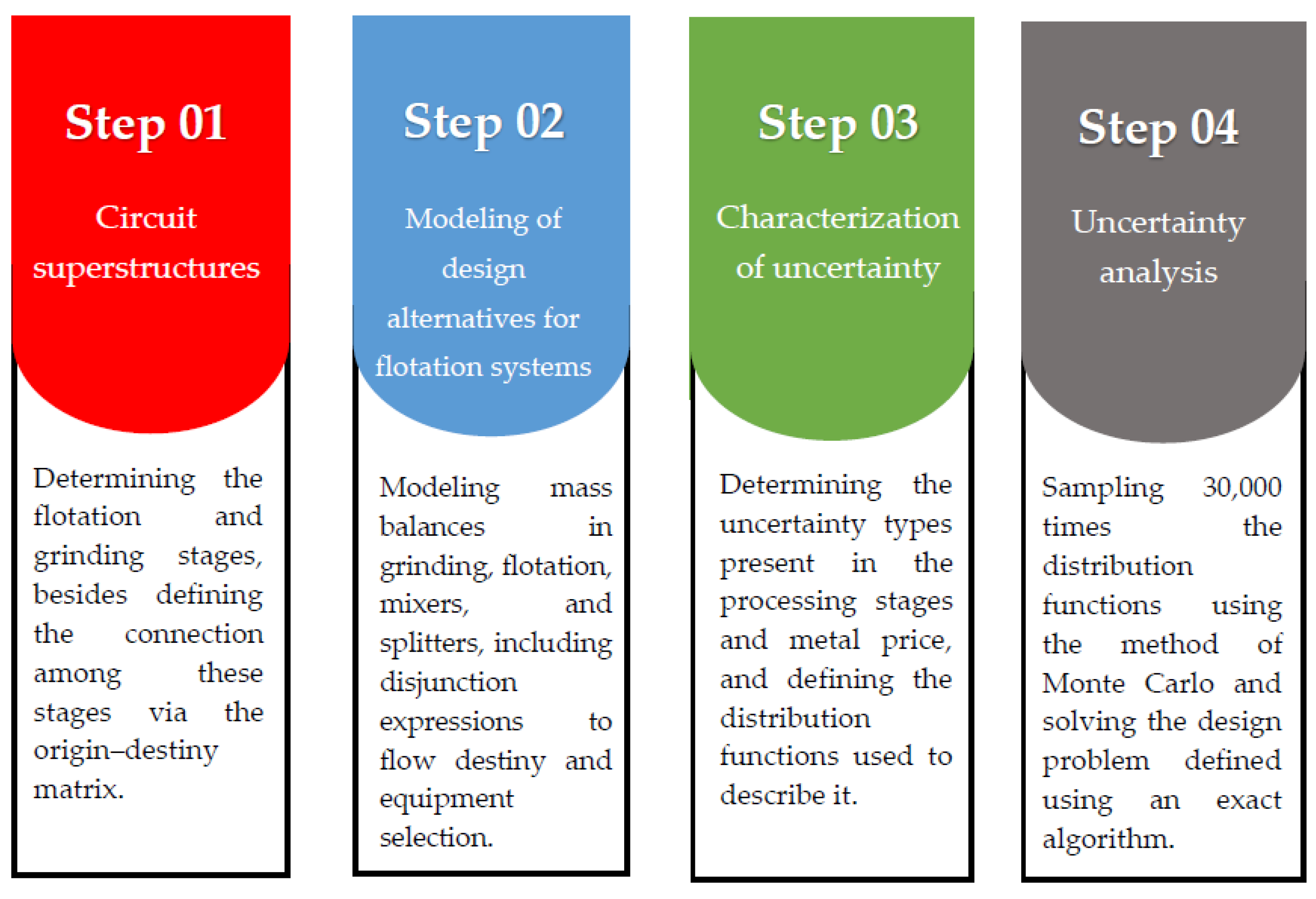
2. Strategy
2.1. Uncertainty Analysis (UA)
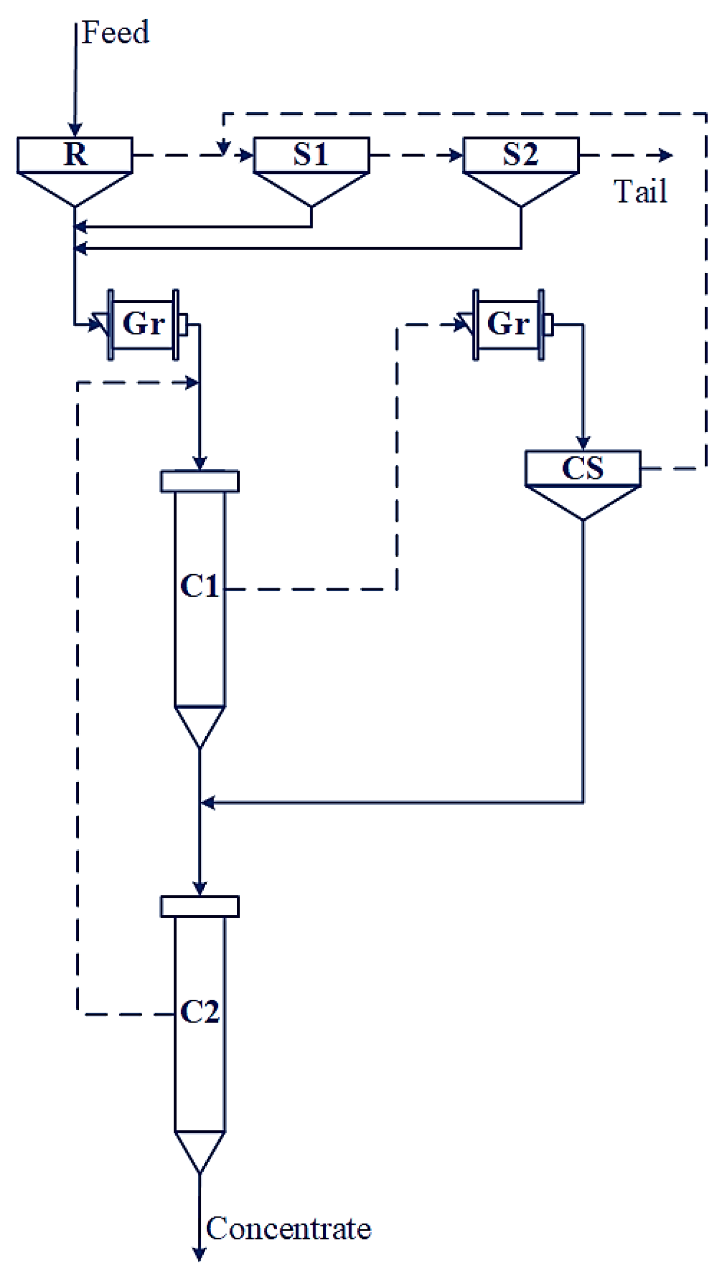
2.2. Superstructure
2.3. Modeling of Design Alternatives
2.4. Optimization Algorithms
3. Applications
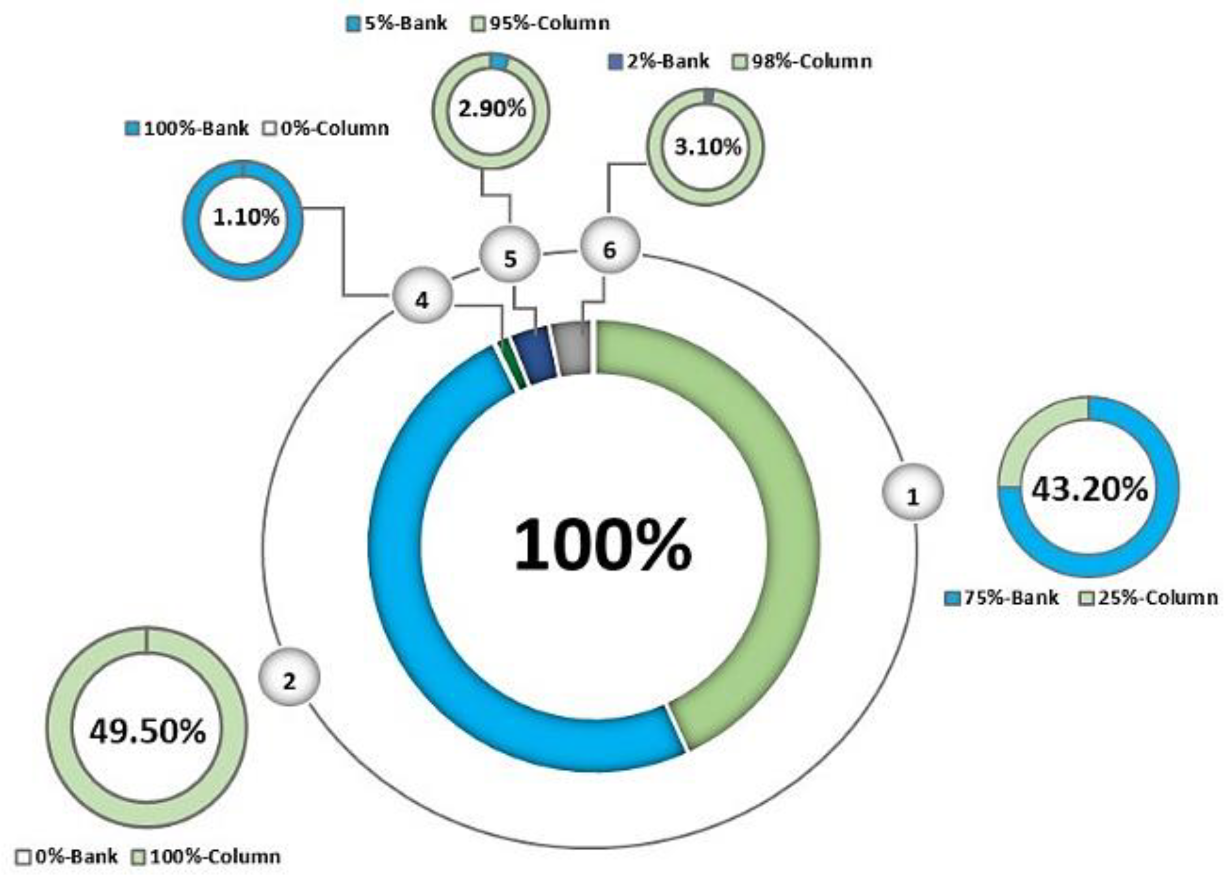
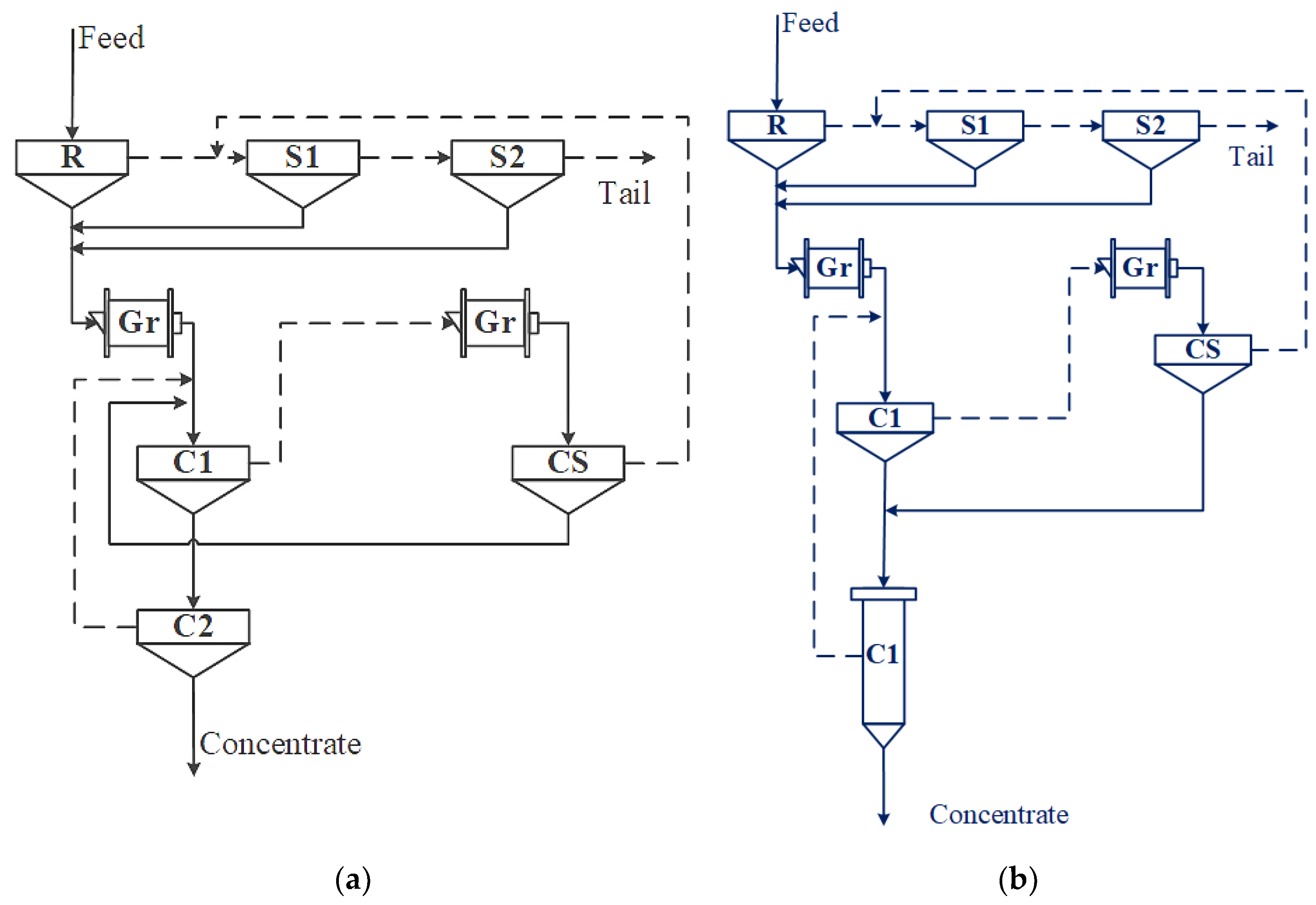
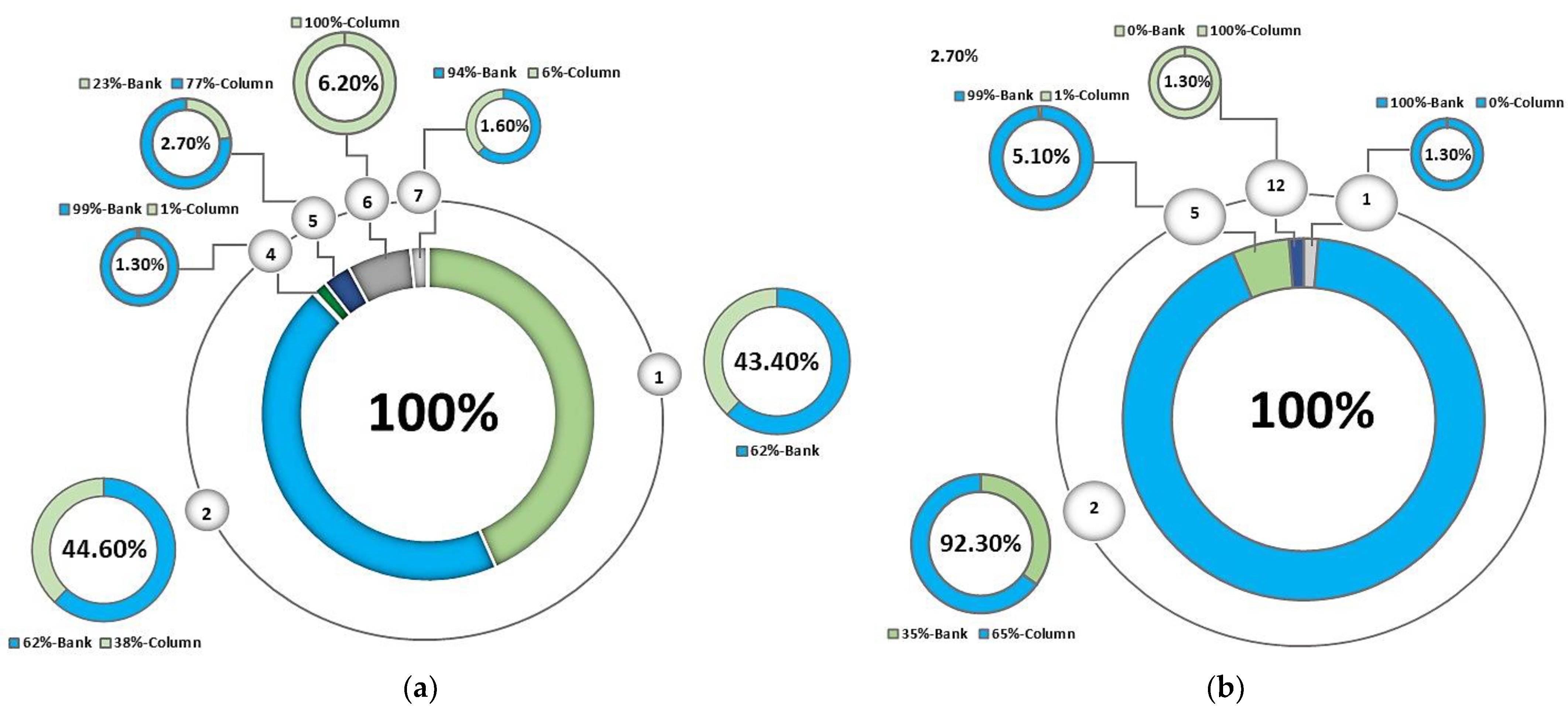
3.1. Uncertainty in Grinding and Flotation Stages, and the Selection of Equipment in the Recleaner Stage
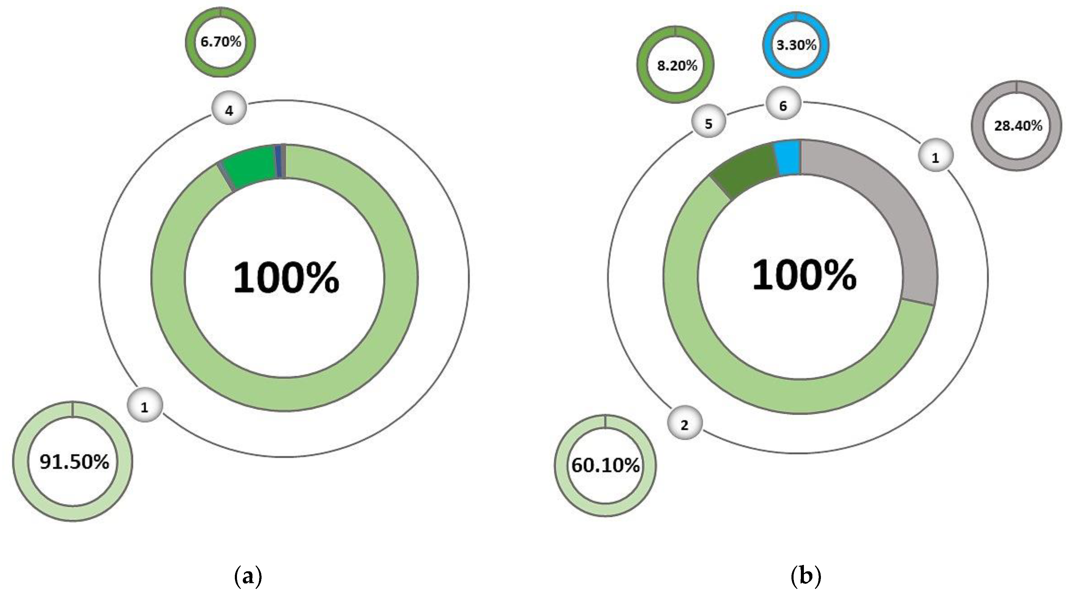
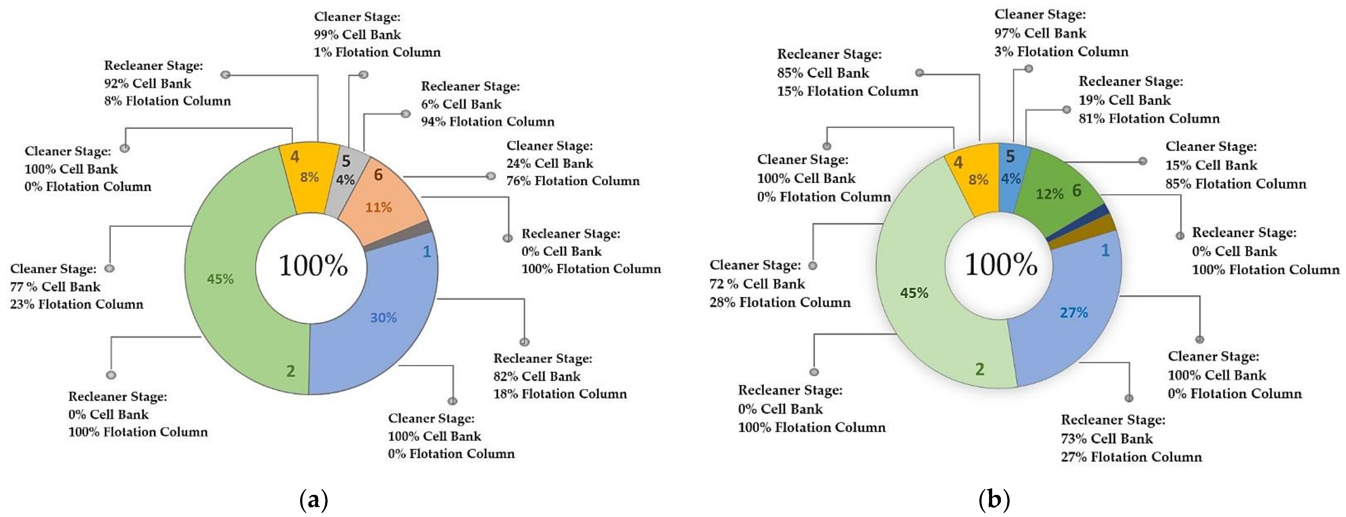
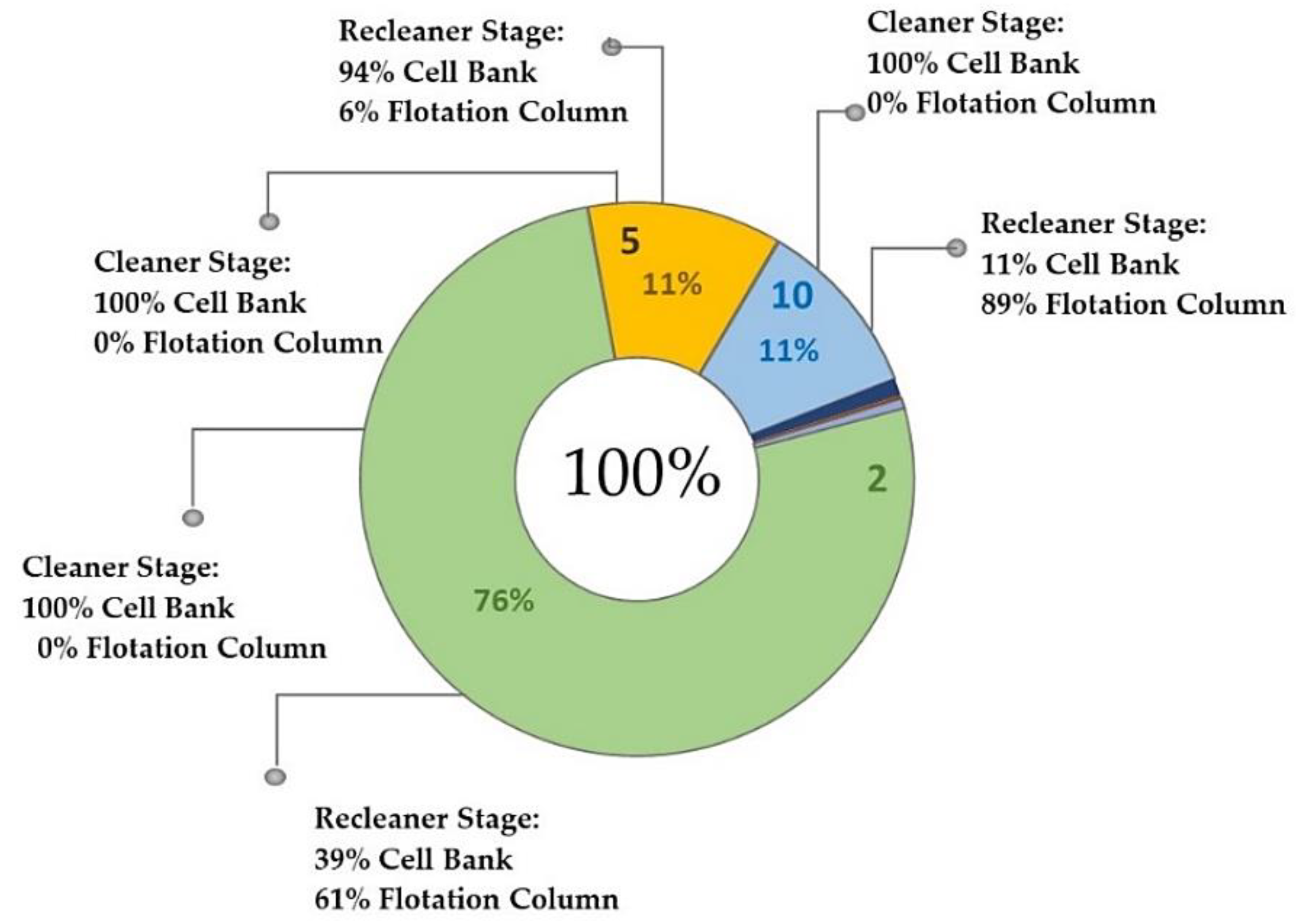
3.2. Uncertainty in Regrinding and Flotation Stages and Selection of Equipment in Cleaner and Recleaner Stages
4. Conclusions
- Using mathematical programming and uncertainty analysis, we determined structures presenting favorable conditions for facing operational and economic uncertainty and consequently conditions favoring flexibility/resilience to determine an optimal operation region;
- The selection of flotation equipment and metal price influenced the percentages of structures in the optimal set. A higher percentage of optimal solutions of one structure implies a greater capacity to face operational and metal price changes. A high copper price reduced the number of primal optimal structures and promoted the appearance of new structures.
Author Contributions
Funding
Data Availability Statement
Acknowledgments
Conflicts of Interest
References
- Hu, W.; Hadler, K.; Neethling, S.J.; Cilliers, J.J. Determining flotation circuit layout using genetic algorithms with pulp and froth models. Chem. Eng. Sci. 2013, 102, 32–41. [Google Scholar] [CrossRef]
- Cisternas, L.A.; Lucay, F.A.; Acosta-Flores, R.; Gálvez, E.D. A quasi-review of conceptual flotation design methods based on computational optimization. Miner. Eng. 2018, 117. [Google Scholar] [CrossRef]
- Mendez, D.A.; Gálvez, E.D.; Cisternas, L.A. State of the art in the conceptual design of flotation circuits. Int. J. Miner. Process. 2009, 90, 1–15. [Google Scholar] [CrossRef]
- Cisternas, L.A.; Jamett, N.; Gálvez, E.D. Approximate recovery values for each stage are sufficient to select the concentration circuit structures. Miner. Eng. 2015. [Google Scholar] [CrossRef]
- Cisternas, L.A.; Acosta-Flores, R.; Lucay, F.; Gálvez, E.D. Mineral Concentration Plants Design Using Rigorous Models. In Computer Aided Chemical Engineering; Zdravko, K., Miloš, B., Eds.; Elsevier: Amsterdam, The Netherlands, 2016; Volume 38, pp. 1461–1466. ISBN 1570-7946. [Google Scholar]
- Calisaya, D.A.; López-Valdivieso, A.; de la Cruz, M.H.; Gálvez, E.E.; Cisternas, L.A. A strategy for the identification of optimal flotation circuits. Miner. Eng. 2016. [Google Scholar] [CrossRef]
- Acosta-Flores, R.; Lucay, F.A.; Cisternas, L.A.; Gálvez, E.D. Two phases optimization methodology for the design of mineral flotation plants including multi-species, bank or cell models. Miner. Metall. Process. J. 2018, 35, 24–34. [Google Scholar]
- Acosta-Flores, R.; Lucay, F.A.; Gálvez, E.D.; Cisternas, L.A. The effect of regrinding on the design of flotation circuits. Miner. Eng. 2020, 156. [Google Scholar] [CrossRef]
- Schena, G.D.; Zanin, M.; Chiarandini, A. Procedures for the automatic design of flotation networks. Int. J. Miner. Process. 1997. [Google Scholar] [CrossRef]
- Cisternas, L.A.; Méndez, D.A.; Gálvez, E.D.; Jorquera, R.E. A MILP model for design of flotation circuits with bank/column and regrind/no regrind selection. Int. J. Miner. Process. 2006. [Google Scholar] [CrossRef]
- Méndez, D.A.; Gálvez, E.D.; Cisternas, L.A. A model of grinding-classification circuit. In Computer Aided Chemical Engineering; Elsevier: Amsterdam, The Netherlands, 2007; Volume 24, pp. 491–496. ISBN 9780444531575. [Google Scholar]
- Sahinidis, N.V. Optimization under uncertainty: State-of-the-art and opportunities. Comput. Chem. Eng. 2004, 28, 971–983. [Google Scholar] [CrossRef]
- Montenegro, M.R.; Sepúlveda, F.D.; Gálvez, E.D.; Cisternas, L.A. Methodology for process analysis and design with multiple objectives under uncertainty: Application to flotation circuits. Int. J. Miner. Process. 2013, 118, 15–27. [Google Scholar] [CrossRef]
- Jamett, N.; Cisternas, L.A.; Vielma, J.P. Solution strategies to the stochastic design of mineral flotation plants. Chem. Eng. Sci. 2015. [Google Scholar] [CrossRef]
- Liang, Y.; He, D.; Su, X.; Wang, F. Fuzzy distributional robust optimization for flotation circuit configurations based on uncertainty theories. Miner. Eng. 2020, 156. [Google Scholar] [CrossRef]
- Cisternas, L.A.; Lucay, F.; Gálvez, E.D. Effect of the objective function in the design of concentration plants. Miner. Eng. 2014, 63, 16–24. [Google Scholar] [CrossRef]
- Grossmann, I.E.; Calfa, B.A.; Garcia-Herreros, P. Evolution of concepts and models for quantifying resiliency and flexibility of chemical processes. Comput. Chem. Eng. 2014. [Google Scholar] [CrossRef]
- Bansal, V.; Perkins, J.D.; Pistikopoulos, E.N. Flexibility analysis and design of dynamic processes with stochastic parameters. Comput. Chem. Eng. 1998. [Google Scholar] [CrossRef]
- Mehrotra, S.P.; Kapur, P.C. Optimal-Suboptimal Synthesis and Design of Flotation Circuits. Sep. Sci. 1974. [Google Scholar] [CrossRef]
- Reuter, M.A.; van Deventer, J.S.J.; Green, J.C.A.; Sinclair, M. Optimal design of mineral separation circuits by use of linear programming. Chem. Eng. Sci. 1988. [Google Scholar] [CrossRef]
- Reuter, M.A.; Van Deventer, J.S.J. The use of linear programming in the optimal design of flotation circuits incorporating regrind mills. Int. J. Miner. Process. 1990. [Google Scholar] [CrossRef]
- Schena, G.; Villeneuve, J.; Noël, Y. A method for a financially efficient design of cell-based flotation circuits. Int. J. Miner. Process. 1996. [Google Scholar] [CrossRef]
- Guria, C.; Verma, M.; Mehrotra, S.P.; Gupta, S.K. Multi-objective optimal synthesis and design of froth flotation circuits for mineral processing, using the jumping gene adaptation of genetic algorithm. Ind. Eng. Chem. Res. 2005, 44, 2621–2633. [Google Scholar] [CrossRef]
- Guria, C.; Verma, M.; Gupta, S.K.; Mehrotra, S.P. Simultaneous optimization of the performance of flotation circuits and their simplification using the jumping gene adaptations of genetic algorithm. Int. J. Miner. Process. 2005, 77, 165–185. [Google Scholar] [CrossRef]
- Mendez, D.A.; Galvez, E.D.; Cisternas, L.A. Modeling of grinding and classification circuits as applied to the design of flotation processes. Comput. Chem. Eng. 2009, 33, 97–111. [Google Scholar] [CrossRef]
- Ghobadi, P.; Yahyaei, M.; Banisi, S. Optimization of the performance of flotation circuits using a genetic algorithm oriented by process-based rules. Int. J. Miner. Process. 2011, 98, 174–181. [Google Scholar] [CrossRef]
- Maldonado, M.; Araya, R.; Finch, J. Optimizing flotation bank performance by recovery profiling. Miner. Eng. 2011. [Google Scholar] [CrossRef]
- Lucay, F.A.; Gálvez, E.D.; Cisternas, L.A. Design of flotation circuits using tabu-search algorithms: Multispecies, equipment design, and profitability parameters. Minerals 2019, 9, 181. [Google Scholar] [CrossRef]
- Helton, J.C.; Burmaster, D.E. Treatment of aleatory and epistemic uncertainty in performance assesments for complex systems. Reliab. Eng. Syst. Saf. 1996, 54, 91–94. [Google Scholar] [CrossRef]
- Helton, J.C.; Oberkampf, W.L. Alternative representations of epistemic uncertainty. Reliab. Eng. Syst. Saf. 2004, 85, 1–10. [Google Scholar] [CrossRef]
- Oberkampf, W. Uncertainty quantification using evidence theory. In Proceedings of the Advanced Simulation Computing Workshop, Albuquerque, MN, USA, 22–23 August 2005. [Google Scholar]
- Cisternas, L.A.; Swaney, R.E. Separation System Synthesis for Fractional Crystallization from Solution Using a Network Flow Model. Ind. Eng. Chem. Res. 1998, 5885, 2761–2769. [Google Scholar] [CrossRef]
- Gálvez, E.D.; Cruz, R.; Robles, P.A.; Cisternas, L.A. Optimization of dewatering systems for mineral processing. Miner. Eng. 2014, 63, 110–117. [Google Scholar] [CrossRef]
- Trujillo, J.Y.; Cisternas, L.A.; Gálvez, E.D.; Mellado, M.E. Optimal design and planning of heap leaching process. Application to copper oxide leaching. Chem. Eng. Res. Des. 2014, 92, 308–317. [Google Scholar] [CrossRef]
- Puchinger, J.; Raidl, G.R. Combining Metaheuristics and Exact Algorithms in Combinatorial Optimization: A Survey and Classification. In Proceedings of the International Work-Conference on the Interplay between Natural and Artificial Computation; Springer: Berlin/Heidelberg, Germany, 2005; pp. 41–53. [Google Scholar]
- InfoMine Copper Price. Available online: http://www.infomine.com/ChartsAndData/ChartBuilder.aspx?z=f&gf=110563.USD.lb&dr=5y&cd=1 (accessed on 15 February 2021).
- Raman, R.; Grossmann, I.E. Modelling and computational techniques for logic based integer programming. Comput. Chem. Eng. 1994, 18, 563–578. [Google Scholar] [CrossRef]
- Kohmuench, J.N.; Mankosa, M.J.; Thanasekaran, H.; Hobert, A. Improving coarse particle flotation using the HydroFloatTM (raising the trunk of the elephant curve). Miner. Eng. 2018, 121, 137–145. [Google Scholar] [CrossRef]


| Stages | ||||||||||
|---|---|---|---|---|---|---|---|---|---|---|
| o | o | x | ||||||||
| o | o | |||||||||
| x | o | x | x | x | o | |||||
| x | x | x | x | o | ||||||
| o | o | o | o | x | o | o | ||||
| o | o | o | o | o | x | |||||
| o | o | o | o | o | ||||||
| o | x | o | o |
| Stages | CPY.f1 | CPY.f2 | CPY.f3 | MIX.f1 | MIX.f2 | MIX.f3 | SC.f1 | SC.f2 | SC.f3 |
|---|---|---|---|---|---|---|---|---|---|
| R | (0.665,0.735) | (0.855,0.945) | (0.760,0.840) | (0.380,0.420) | (0.665,0.735) | (0.570,0.630) | (0.048,0.053) | (0.095,0.105) | (0.048,0.053) |
| C1, cell | (0.475,0.525) | (0.665,0.735) | (0.475,0.525) | (0.190,0.210) | (0.475,0.525) | (0.285,0.315) | (0.048,0.053) | (0.057,0.063) | (0.048,0.053) |
| C2, cell | (0.475,0.525) | (0.665,0.735) | (0.475,0.525) | (0.190,0.210) | (0.475,0.525) | (0.285,0.315) | (0.048,0.053) | (0.057,0.063) | (0.048,0.053) |
| C1, col | (0.285,0.315) | (0.380,0.420) | (0.285,0.315) | (0.190,0.210) | (0.285,0.315) | (0.190,0.210) | (0.024,0.026) | (0.024,0.026) | (0.024,0.026) |
| C2, col | (0.285,0.315) | (0.380,0.420) | (0.285,0.315) | (0.190,0.210) | (0.285,0.315) | (0.190,0.210) | (0.024,0.026) | (0.024,0.026) | (0.024,0.026) |
| S1 | (0.665,0.735) | (0.855,0.945) | (0.760,0.840) | (0.380,0.420) | (0.665,0.735) | (,0570,0.630) | (0.048,0.053) | (0.095,0.105) | (0.048,0.053) |
| S2 | (0.665,0.735) | (0.855,0.945) | (0.760,0.840) | (0.380,0.420) | (0.665,0.735) | (,0570,0.630) | (0.095,0.105) | (0.190,0.210) | (0.095,0.105) |
| CS | (0.665,0.735) | (0.855,0.945) | (0.760,0.840) | (0.380,0.420) | (0.665,0.735) | (,0570,0.630) | (0.095,0.105) | (0.190,0.210) | (0.095,0.105) |
| CPY.f1 | CPY.f2 | CPY.f3 | MIX.f1 | MIX.f2 | MIX.f3 | SC.f1 | SC.f2 | SC.f3 | |
|---|---|---|---|---|---|---|---|---|---|
| CPY.f1 | (0.05,0.15) | (0.35,0.45) | (0.45,0.55) | ||||||
| CPY.f2 | (0.15,0.25) | (0.75,0.85) | |||||||
| CPY.f3 | 1 | ||||||||
| MIX.f1 | (0.05,0.15) | (0.05,0.15) | (0.25,0.30) | (0.25,0.30) | (0.05,0.15) | (0.00,0.10) | (0.00,0.075) | (0.00,0.075) | |
| MIX.f2 | (0.05,0.15) | (0.55,0.65) | (0.05,0.15) | (0.15,0.25) | |||||
| MIX.f3 | 1 | ||||||||
| SC.f1 | 1 | ||||||||
| SC.f2 | (0.190,0.210) | (0.095,0.105) |
| CPY.f1 | CPY.f2 | CPY.f3 | MIX.f1 | MIX.f2 | MIX.f3 | SC.f1 | SC.f2 | SC.f3 | |
|---|---|---|---|---|---|---|---|---|---|
| CPY.f1 | (0.048,0.053) | (0.285,0.315) | (0.615,0.682) | ||||||
| CPY.f2 | (0.285,0.315) | (0.665,0.735) | |||||||
| CPY.f3 | 1 | ||||||||
| MIX.f1 | (0.19,0.21) | (0.19,0.21) | (0.095,0.105) | (0.19,0.21) | (0.19,0.21) | (0.0475,0.0525) | (0.0237,0.0262) | (0.0237,0.0262) | |
| MIX.f2 | (0.095,0.105) | (0.285,0.315) | (0.095,0.105) | (0.21,0.19) | (0.19,0.21) | (0.095,0.105) | |||
| MIX.f3 | (0.19,0.21) | (0.38,0.42) | (0.38,0.42) | ||||||
| SC.f1 | (0.095,0.105) | (0.38,0.42) | (0.475,0.525) | ||||||
| SC.f2 | (0.665,0.735) | (0.285,0.315) |
Publisher’s Note: MDPI stays neutral with regard to jurisdictional claims in published maps and institutional affiliations. |
© 2021 by the authors. Licensee MDPI, Basel, Switzerland. This article is an open access article distributed under the terms and conditions of the Creative Commons Attribution (CC BY) license (https://creativecommons.org/licenses/by/4.0/).
Share and Cite
Lucay, F.A.; Acosta-Flores, R.; Gálvez, E.D.; Cisternas, L.A. Toward the Operability of Flotation Systems under Uncertainty. Minerals 2021, 11, 646. https://doi.org/10.3390/min11060646
Lucay FA, Acosta-Flores R, Gálvez ED, Cisternas LA. Toward the Operability of Flotation Systems under Uncertainty. Minerals. 2021; 11(6):646. https://doi.org/10.3390/min11060646
Chicago/Turabian StyleLucay, Freddy A., Renato Acosta-Flores, Edelmira D. Gálvez, and Luis A. Cisternas. 2021. "Toward the Operability of Flotation Systems under Uncertainty" Minerals 11, no. 6: 646. https://doi.org/10.3390/min11060646
APA StyleLucay, F. A., Acosta-Flores, R., Gálvez, E. D., & Cisternas, L. A. (2021). Toward the Operability of Flotation Systems under Uncertainty. Minerals, 11(6), 646. https://doi.org/10.3390/min11060646