Seismic Wave Speeds Derived from Nuclear Resonant Inelastic X-ray Scattering for Comparison with Seismological Observations

Abstract

Nuclear resonant inelastic X-ray scattering (NRIXS) experiments have been applied to Earth materials, and the Debye speed is often related to the material’s seismic wave speeds. However, for anisotropic samples, the Debye speed extracted from NRIXS measurements is not equal to the Debye speed obtained using the material’s isotropic seismic wave speeds. The latter provides an upper bound for the Debye speed of the material. Consequently, the acoustic wave speeds estimated from the Debye speed extracted from NRIXS (Nuclear Resonant Inelastic X-ray Scattering) measurements are underestimated compared to the material’s true seismic wave speeds. To illustrate the differences, the effects of various assumptions used to estimate the Debye speed, as well as seismic wave speeds, are examined with iron alloys at Earth’s inner core conditions. For the case of pure iron, the variation of the crystal orientation relative to the incoming X-ray beam causes a $40\%$ variation in the measured Debye speed, and leads to 3% and 31% underestimation in the compressional and shear wave speeds, respectively. Based upon various iron alloys, the error in the inferred seismic shear wave speed strongly depends upon the strength of anisotropy that can be quantified. We can also derive Debye speeds based upon seismological observations such as the PREM (Preliminary Reference Earth Model) and inner core anisotropy model. We show that these seismically derived Debye speeds are upper bounds for Debye speeds obtained from NRIXS experiments and that interpretation of the Debye speeds from the NRIXS measurements in terms of seismic wave speeds should be done with utmost caution.

1. Introduction

Advances in instrumentation and experimental techniques are allowing for rapid improvement in the use of lattice dynamics to determine the elastic moduli of materials at high pressure (e.g., [1,2]). Inelastic scattering of synchrotron radiation is used to probe the mechanical properties of condensed matter. The importance of this method over other measurements such as ultrasonic methods or Brillouin scattering lies in its ability to be used on small samples under extreme pressure conditions, and has already been successfully applied to Earth materials (e.g., [3]). A review and critical comparison of the variety of techniques and methodologies used to measure sound velocities in metals at megabar pressures can be found in Antonangeli & Ohtani [4], and references therein. Nuclear resonant inelastic X-ray scattering experiments (NRIXS) directly probe the vibrational structure of solids (e.g., [5,6,7,8]), and these measurements provide the Fourier-transformed self-intermediate scattering function from which the energy levels of the excited acoustic phonons and the Debye speed can be extracted (e.g., [3]). The Debye speed is a direct link to the material’s elastic properties.

One application of NRIXS measurements, which is of particular interest to geophysics, is to understand the alloying effects of nickel and light elements (e.g., S, Si, C, H, etc.) on the elastic properties of iron at inner core conditions. Due to the extreme high pressures and temperatures at the center of the Earth, it has been historically difficult to obtain experimental measurements of the acoustic properties of candidate materials to compare with the seismically observed elastic properties. Recent applications of NRIXS to iron alloy samples in a diamond anvil cell reveal that NRIXS measurements provide an exciting new opportunity to experimentally constrain geophysical models of the Earth’s inner core.

This study builds upon the work of Anderson [9,10], who suggested that the Debye speed could be estimated from single crystal elastic constants, and developed techniques which used theories from lattice dynamics to link optical vibrations of a solid to its Debye speed to determine seismic shear wave speeds of materials at high pressures. We show that the Debye speeds calculated from the seismic wave speeds of polycrystalline materials composed of randomly oriented anisotropic crystal with bulk or macroscopically isotropic properties (e.g., powdered samples) yields an upper bound for the material’s Debye speed. Furthermore, we show that increasing the strength of anisotropy of a material decreases its Debye speed, even when its bulk isotropic properties remain unchanged.

The study highlights the difficulty of comparing NRIXS derived Debye speeds with seismically observed wave speeds. This is demonstrated by showing the effects of the various approximations to the calculation of the Debye speed for the case of several iron alloys at inner core pressures and temperatures. These results are crucial for using NRIXS measurements of the Debye speed in geophysical applications, and a new methodology is derived that avoids the isotropic assumptions which are currently a large source of error in procedures which extract seismic wave speeds from NRIXS measurements.

2. Theory

Mechanical information can be extracted from phonon density of states $\nu \left(E\right)$, since, at low energies, only the acoustic phonon modes are excited by the incident photon and participate in the inelastic absorption. This low energy portion of the density of states exhibits Debye-like behavior in which it is linear with the square of the energy [5]. In the harmonic lattice approximation [11], the density of states can be written as

$$\nu \left(E\right)=\frac{M}{\rho }\frac{E^2}{2{\pi }^2{\hslash }^3}\frac{1}{v_D^3},$$

(1)

where M is the mass of the resonant nucleus, $\rho$ is the density of the solid, $2\pi \hslash$ is Plank’s constant, E is the energy of the photon relative to the resonance energy of the nuclear transition, and $v_D$ is the Debye speed. The Debye speed is defined as an average over all wave speeds such that

$$\frac{1}{v_D^3}=\frac{1}{3}\sum _{m=1}^3\int \frac{d{\mathsf{\Omega }}_{\widehat{\mathbf{q}}}}{4\pi }\frac{1}{c_m^3\left(\widehat{\mathbf{q}}\right)},$$

(2)

where $c_m\left(\widehat{\mathbf{q}}\right)$ is the wave speed of an acoustic phonon of type m (e.g., longitudinal or horizontally/vertically polarized transverse waves) propagating in the direction of the unit vector $\widehat{\mathbf{q}}$, and $d{\mathsf{\Omega }}_{\widehat{\mathbf{q}}}$ is the corresponding differential solid angle element. Note that throughout this manuscript, c denotes acoustic wave speeds, and v represents quantities derived from the phonon density of states. For the isotropic elastic materials, there is no directional dependence of the wave speeds, and the expression for the Debye speed $v_D$ can be simplified in terms of its compressional ($c_p$) and shear ($c_s$) wave speeds as

$$\frac{1}{v_D^3}=\frac{1}{3}\sum _{m=1}^3\frac{1}{c_m^3}=\frac{1}{3}\left(\frac{1}{c_p^3}+\frac{2}{c_s^3}\right).$$

(3)

Note that the factor of 2 arises from the fact that the shear modes are degenerate.

The observations from nuclear resonant inelastic scattering provide measurements of the “projected” density of states $g(E,\widehat{\mathbf{k}})$, also referred to as the “partial” density of states which is given by (e.g., [8,12])

$$g(E,\widehat{\mathbf{k}})=\frac{M}{\rho }\frac{E^2}{2{\pi }^2{\hslash }^3}\frac{1}{v_{\widehat{\mathbf{k}}}^3},$$

(4)

where $v_{\widehat{\mathbf{k}}}$ is the “projected mean wave speed”, that is, the wave speeds weighted by the projection of the incident photon unit wave vector $\widehat{\mathbf{k}}$ (Figure 1) on to the unit phonon polarization vectors of type m, ${\widehat{\mathbf{p}}}_m$. It is defined as

$$\frac{1}{v_{\widehat{\mathbf{k}}}^3}=\sum _{m=1}^3\int \frac{d{\mathsf{\Omega }}_{\widehat{\mathbf{q}}}}{4\pi }\frac{{\left|\widehat{\mathbf{k}}·{\widehat{\mathbf{p}}}_m\left(\widehat{\mathbf{q}}\right)\right|}^2}{c_m^3\left(\widehat{\mathbf{q}}\right)},$$

(5)

where $c_m$ is the wave speed for acoustic phonon of type m, and $0\le {\left|\widehat{\mathbf{k}}·{\widehat{\mathbf{p}}}_m\left(\widehat{\mathbf{q}}\right)\right|}^2\le 1$ for all $\widehat{\mathbf{k}}$ and $\widehat{\mathbf{q}}$. In practice, the slope of the linear fit to the experimentally observed projected phonon density of states $\nu$ versus $E^2$ is used to estimate $v_{\widehat{\mathbf{k}}}$.

The projected mean wave speed, $v_{\widehat{\mathbf{k}}}$, is the link between the nuclear resonant derived measurements of the phonon density of states and the material’s elastic constants. In this case, the experimentally observable $g(E,\widehat{\mathbf{k}})$ is proportional to $v_{\widehat{\mathbf{k}}}^{-3}$, which is related to the inverse cubed acoustic wave speeds $c_m^{-3}$ (Equation (5)). However, the sample orientation with respect to the wave vector is not easily obtained, and the samples are often polycrystalline. For the case of randomly oriented aggregates (e.g., powdered samples), the experimental result is well represented by averaging over the incident wave vector direction $\widehat{\mathbf{k}}$ [8,12]. The average over the unit sphere of an arbitrary function $g(\theta ,\varphi )$ is denoted by $〈g(\theta ,\varphi )〉=\int g(\theta ,\varphi )d\mathsf{\Omega }/4\pi =\int g(\theta ,\varphi )sin\theta d\theta d\varphi /4\pi$ where $\mathsf{\Omega }$ is the solid angle. The experimentally derived partial density of state is

$$g(E,\widehat{\mathbf{k}})=\frac{M}{\rho }\frac{E^2}{2{\pi }^2{\hslash }^3}〈\frac{1}{v_{\widehat{\mathbf{k}}}^3}〉,$$

(6)

and can be directly related to the theoretical Debye speed $v_D$ (see Appendix C) by

$$〈\frac{1}{v_{\widehat{\mathbf{k}}}^3}〉=\int \frac{d{\mathsf{\Omega }}_{\widehat{\mathbf{k}}}}{4\pi }\frac{1}{v_{\widehat{\mathbf{k}}}^3}=\frac{1}{v_D^3}.$$

(7)

while the mean projected sound speed $v_{\widehat{\mathbf{k}}}$ has been averaged over the incident wave vector $\widehat{\mathbf{k}}$ and the directional dependence of the excitation of the phonon modes has been removed, the acoustic wave speeds $c_m\left(\widehat{\mathbf{q}}\right)$ still depend on their propagation direction $\widehat{\mathbf{q}}$.

Alternative Expressions for the Debye Speed under Various Simplifying Assumptions

While randomly oriented anisotropic crystals create a material that appears isotropic in its bulk or macroscopic acoustic properties, the Debye speed measured from this material is not equivalent to the Debye speed that would be obtained from a material with equivalent isotropic properties. This distinction is critical for geophysical applications which seek to derive the seismic P- and S-wave speeds of materials from NRIXS experiments. The discrepancy arises since the procedure commonly used to extract these wave speeds assumes that the material is isotropic (e.g., [3]), while the materials being measured are often anisotropic.

In order to extract isotropic properties such as elastic moduli and seismic wave speeds from anisotropic materials, a mapping of the anisotropic tensor elements to isotropic wave speeds is required. Mathematically, there are several schemes for generating the isotropic elastic moduli from anisotropic fourth-order elasticity tensors under various assumptions such as constant stress condition (e.g., Reuss average). When it comes to constraints for the Earth’s interior, the isotropic average information is provided by seismological observations rather than from elasticity tensor with an assumption. Hence, it is critical to understand how the seismological data averages components of the elasticity tensor that ultimately result in isotropic models such as the Preliminary Reference Earth Model [13]. Delbridge & Ishii [14] shows that the relevant averaging scheme for seismic wave propagation is equivalent to the Voigt average, and the elasticity tensor can be written as

$${\mathsf{\Lambda }}_{ijkl}=\left({\kappa }_0^V-\frac{2}{3}{\mu }_0^V\right){\delta }_{ij}{\delta }_{kl}+{\mu }_0^V\left({\delta }_{ik}{\delta }_{jl}+{\delta }_{il}{\delta }_{jk}\right)+{\gamma }_{ijkl},$$

(8)

where the subscripts i,j,k, and l are used as Einstein notation and ${\delta }_{ij}$ is the Kronecker delta. The first two terms on the right-hand side describe the isotropic behaviour arising from isotropic contributions while the last term, ${\gamma }_{ijkl}$, describes the anisotropic deviations from isotropy. The superscript V denotes that Voigt averaging schemes are used to obtain the bulk and shear moduli, ${\kappa }_0^V$ and ${\mu }_0^V$. The isotropic seismic waves speeds are related to these elastic moduli as

$$\rho c_p^2={\kappa }_0^V+\frac{4}{3}{\mu }_0^V\mathrm{and}\rho c_s^2={\mu }_0^V,$$

(9)

where $c_p$ and $c_s$ are the material’s compressional and shear wave speeds, respectively. The seismic wave speeds allow us to estimate the Debye speed under the assumption that it is equivalent to isotropic wave speeds that appear in Equation (3). We denote this Debye speed as $v_D^V$ to indicate the Debye speed of a material based upon seismic wave speeds.

We can write another expression for the Debye speed by assuming that the directionally averaged wave speeds can be used as the isotropic wave speeds, that is,

$$\frac{1}{v_D^3}\approx \frac{1}{{\overline{v}}_D^3}\equiv \frac{1}{3}\sum _{m=1}^3{〈c_m^2〉}^{-3/2}=\frac{1}{3}\left(\frac{1}{{〈c_1^2〉}^{3/2}}+\frac{1}{{〈c_2^2〉}^{3/2}}+\frac{1}{{〈c_3^2〉}^{3/2}}\right).$$

(10)

these directionally averaged elastic properties are related to the seismic wave speeds and Voigt moduli as (see Appendix A)

$$\rho 〈c_1^2〉=\rho c_p^2={\kappa }_0^V+\frac{4}{3}{\mu }_0^V,\mathrm{and}\frac{1}{2}\rho \left(〈c_2^2〉+〈c_3^2〉\right)=\rho c_s^2={\mu }_0^V.$$

(11)

For isotropic materials $v_D={\overline{v}}_D=v_D^V$, but for anisotropic materials, ${\overline{v}}_D$, and $v_D^V$ may deviate from $v_D$. We seek a relationship between them in order to understand the implications of various assumptions employed when relating a material’s Debye speed to its elastic properties, and hence to associated seismic wave speeds. The Debye speed ($v_D$) is given by Equation (2), hence

$$\frac{1}{v_D^3}=\frac{1}{3}\sum _{m=1}^3\int \frac{d{\mathsf{\Omega }}_{\widehat{\mathbf{q}}}}{4\pi }\frac{1}{c_m^3\left(\widehat{\mathbf{q}}\right)}=\frac{1}{3}\sum _{m=1}^3\int \frac{d\mathsf{\Omega }}{4\pi }{\left(f_m\right)}^{-3/2}=\frac{1}{3}\sum _{m=1}^3〈f_m^{-3/2}〉,$$

(12)

where $f_m=c_m^2$. On the other hand, the Debye speed based upon the material’s seismic wave speeds (Equation (10)) can be written as

$$\frac{1}{{\overline{v}}_D^3}=\frac{1}{3}\sum _{m=1}^3{〈f_m〉}^{-3/2}.$$

(13)

since $f_m$ is strictly positive and $f_m\to f_m^{-3/2}$ is convex for $f_m>0$, Jensen’s inequality [15,16] tells us that

$$〈f_m^{-3/2}〉\ge {〈f_m〉}^{-3/2},$$

(14)

which implies that

$$\frac{1}{3}\sum _{m=1}^3〈f_m^{-3/2}〉\ge \frac{1}{3}\sum _{m=1}^3{〈f_m〉}^{-3/2}.$$

(15)

Furthermore, we can show that

$$\frac{1}{{〈c_1^2〉}^{3/2}}+\frac{1}{{〈c_2^2〉}^{3/2}}+\frac{1}{{〈c_3^2〉}^{3/2}}\ge \frac{1}{{〈c_1^2〉}^{3/2}}+\frac{2}{{\left(\frac{〈c_2^2〉+〈c_3^2〉}{2}\right)}^{3/2}}=\frac{1}{c_p^3}+\frac{2}{c_s^3},$$

(16)

which leads to the conclusion that

$$\frac{1}{3}\sum _{m=1}^3〈f_m^{-3/2}〉\ge \frac{1}{3}\sum _{m=1}^3{〈f_m〉}^{-3/2}\ge \frac{1}{3}\left(\frac{1}{c_p^3}+\frac{2}{c_s^3}\right).$$

(17)

This is equivalent to

$$\frac{1}{v_D^3}\ge \frac{1}{{\overline{v}}_D^3}\ge \frac{1}{{v_D^V}^3},$$

(18)

from which we can write the desired inequality relating the Debye speed $v_D$ to its approximation using the seismic wave speeds $v_D^V$

$$v_D\le v_D^V.$$

(19)

Physically, this equation implies that the Debye speed of anisotropic materials ($v_D$) is not equivalent to the Debye speed estimated from that material’s seismic wave speeds ($v_D^V$), and that the latter is an upper bound to the former. Consequently, since the commonly used procedure to estimate seismic wave speeds from NRIXS experiments assumes that the Debye speed can be related directly to the material’s seismic wave speeds, that is, equality in Equation (19), these speeds are often underestimated.

3. Results and Discussion

In order to explore the effect of analyzing anisotropic single crystals and polycrystalline aggregates, elastic tensor elements of five iron alloys with hexagonal-close packed (hcp) [17,18,19,20] and one with a body-centered cubic (bcc) [21] structure are considered (

Table 1. The elastic constants and seismic wave speeds of iron alloys (column 1; [17,18,19,20,21]). The alloy’s density in $\mathrm{g}/{\mathrm{cm}}^3$ ($\rho$; column 2), seismic compressional wave speed in km/s ($c_p$; column 3), shear wave speed in km/s ($c_s$; column 4), the strength of anisotropy ($A^L$; column 6; [22]), and the elastic tensor elements in GPa (columns 6 through 11) are summarized.

Material	$\mathit{\rho }$	${\mathit{c}}_{\mathit{p}}$	${\mathit{c}}_{\mathit{s}}$	${\mathit{A}}^{\mathit{L}}$	${\mathit{c}}_{11}$	${\mathit{c}}_{33}$	${\mathit{c}}_{13}$	${\mathit{c}}_{44}$	${\mathit{c}}_{66}$	${\mathit{c}}_{12}$
hcp Fe	13.0	11.8	3.9	1.5	2150	1685	990	140	60	2030
hcp Fe-Si	13.1	11.3	3.9	0.3	1674	1855	1120	176	137	1400
hcp Fe-Si-Ni	12.5	11.8	3.3	1.4	1816	1964	1224	80	49	1718
hcp Fe-Si-C	13.1	11.6	3.7	0.6	1712	2066	1263	164	91	1530
hcp Fe-S-C	13.1	11.8	4.2	0.3	1831	2091	1214	183	173	1485
bcc Fe-Si	13.6	11.5	4.2	1.7	1562	1562	1448	366	366	1448

). The five hcp iron materials are—a pure iron at $6000{}^{\circ }\mathrm{K}$ with a density of $13.0\mathrm{g}/{\mathrm{cm}}^3$[17], a Fe-Si alloy with 12.5 at% Si at 360 GPa and $6900{}^{\circ }\mathrm{K}$[20], a Fe-Ni-Si alloy with 10 at% Ni and 21.25 at% Si with density of $12.5\mathrm{g}/{\mathrm{cm}}^3$ at 360 GPa and $6500{}^{\circ }\mathrm{K}$[18], a Fe-Si-C alloy with 4.2 at% Si and 0.7 at% C with density of $13.1\mathrm{g}/{\mathrm{cm}}^3$ at 360 GPa and $6500{}^{\circ }\mathrm{K}$[19], and a Fe-S-C alloy with 2.1 at% S and 0.7 at% C with density of $13.1\mathrm{g}/{\mathrm{cm}}^3$ at 360 GPa and $6500{}^{\circ }\mathrm{K}$ [19]. The last material considered is a Fe-Si bcc alloy at 360 GPa and $6000{}^{\circ }\mathrm{K}$ with density of $13.6\mathrm{g}/{\mathrm{cm}}^3$ [21]. The seismic wave speeds $c_p$ and $c_s$ are calculated from the elastic tensor elements (Table 1) such that they are comparable with the seismically observed wave speeds [14].

To investigate how various parameters are influenced by anisotropy, we introduce an absolute measure of anisotropy, $A^L$, that quantifies the log-Euclidean distance between the Voigt averaged elastic tensor $〈{\mathsf{\Lambda }}_{ijkl}〉$ and the Reuss averaged elastic tensor ${〈{\mathsf{\Lambda }}_{ijkl}^{-1}〉}^{-1}$[22,23]. The log-Euclidean distance may be written in terms of the Voigt and Reuss averaged isotropic moduli ${\kappa }_0$ and ${\mu }_0$ as [22]

$$A^L=\sqrt{5ln{\left(\frac{{\mu }_0^V}{{\mu }_0^R}\right)}^2+ln{\left(\frac{{\kappa }_0^V}{{\kappa }_0^R}\right)}^2},$$

(20)

where the superscripts V and R denote the Voigt and Reuss averages, respectively. The Voigt and Reuss averages coincide for the case of isotropic material [24], and for this case, $A^L$ yields a value of zero.

3.1. Variations in the Debye Speed

We first calculate the mean projected wave speed $v_{\widehat{\mathbf{k}}}$ for all possible incident photon wave vectors $\widehat{\mathbf{k}}$ (Equation (5)). This requires numerically calculating the wave speeds (eigenvalues) and polarization vectors (eigenvectors) as described in the Appendix A, and then numerically integrating over the phonon propagation directions, $\widehat{\mathbf{q}}$ (Equation (5)). The minimum and maximum values represent the spread of possible mean projected wave speeds that may be measured for a given single crystal sample due to changes in orientation of the crystal with respect to the incoming X-ray beam (Figure 1,

Table 2. Exact and approximate Debye speeds calculated from the elastic tensor elements of hcp and bcc iron alloys (column 1). Percent variation (column 2) of the difference of the extreme values of $v_{\widehat{\mathbf{k}}}$ (column 3) with respect to the average of the extreme values due to variations in $\widehat{\mathbf{k}}$ are given. The true Debye speed $v_D$ (column 4), and the approximate Debye speed obtained using the analytical expressions for $c_m$ given in the Appendix A (column 5) are compared. The last three columns give the values obtained using Equation (3) where the elastic moduli $\kappa$ and $\mu$ are estimated using the Voigt, Reuss, and Voigt-Reuss-Hill averages, respectively. The speeds are all in units of km/s.

Material	$\pm \%$	$\left[min{\mathit{v}}_{\widehat{\mathit{k}}},max{\mathit{v}}_{\widehat{\mathit{k}}}\right]$	${\mathit{v}}_{\mathit{D}}$	${\mathit{v}}_{\mathit{D}}^{\mathit{q}}$	${\mathit{v}}_{\mathit{D}}^{\mathit{V}}$	${\mathit{v}}_{\mathit{D}}^{\mathit{R}}$	${\mathit{v}}_{\mathit{D}}^{\mathit{V}\mathit{R}\mathit{H}}$
hcp Fe	$40\%$	$\left[3.07,4.60\right]$	3.35	3.35	4.45	3.18	3.87
hcp Fe-Si	$16\%$	$\left[4.04,4.76\right]$	4.23	4.22	4.47	4.16	4.32
hcp Fe-Si-Ni	$37\%$	$\left[2.66,3.85\right]$	2.89	2.96	3.78	2.77	3.32
hcp Fe-Si-C	$28\%$	$\left[3.53,4.66\right]$	3.79	3.83	4.21	3.67	3.95
hcp Fe-S-C	$13\%$	$\left[4.38,4.97\right]$	4.54	4.56	4.77	4.47	4.62
bcc Fe-Si	$0\%$	$\left[4.04,4.04\right]$	4.04	4.04	4.79	3.33	4.13

). For the transversely isotropic hcp materials considered in this study, the maximum projected mean wave speed corresponds to an incident X-ray beam aligned along the axis of symmetry, and the minimum corresponds to an incident X-ray beam in the plane perpendicular to the axis of symmetry. The range in $v_{\widehat{\mathbf{k}}}$ caused by this orientation effect is proportional to the strength of anisotropy, with a $20\%$ increase per unit of anisotropy (Figure 2). For the hcp pure iron, $v_{\widehat{\mathbf{k}}}$ varies by about $40\%$, whereas for the less anisotropic hcp Fe-S-C alloy, it is only $13\%$ (Table 2). As expected from the symmetry in the scattering matrix for cubic materials [11], the projected mean wave speed $v_{\widehat{\mathbf{k}}}$ is constant and is identical to the Debye speed for the bcc Fe-Si alloy (Table 2).

In order to examine the Debye speed $v_D={〈v_{\widehat{\mathbf{k}}}^{-3}〉}^{-1/3}$ (Equation (7)) of powdered samples, an additional integration over the wave vector $\widehat{\mathbf{k}}$ is needed. Because of cubic symmetry, $v_{\widehat{\mathbf{k}}}=v_D$ for the bcc Fe-Si alloy (Table 1). The Fe-Si-Ni alloy which has the lowest seismic shear wave speed of $3.3\mathrm{km}/\mathrm{s}$ (Table 1) results in the lowest $v_D$ value of $3.0\mathrm{km}/\mathrm{s}$, and the hcp Fe-S-C alloy which had the highest seismic shear wave speed $4.2\mathrm{km}/\mathrm{s}$ results in the highest $v_D$ value of $4.6\mathrm{km}/\mathrm{s}$. The Debye speed $v_D$ in Equation (7) can also be calculated approximately using the first-order propagation and polarization vectors (see Appendix A) and obtaining the corresponding wave speeds which we denote by $v_D^q$. This procedure may either be done by numerical matrix multiplication, or for hexagonal and cubic symmetries, using the analytical expressions as described in the Appendix A. Use of these analytical expressions for wave speeds and associated polarization vectors to calculated Debye speed is only valid for weakly anisotropic materials, however, the approximate values of $v_D^q$ are nearly identical to the exact values $v_D$ (Table 2). Even for the case of the highly anisotropic materials, such as pure iron, the error is less than half a percent. On the other hand, Debye speeds based upon various isotropic averages, $v_D^V$, $v_D^R$, and $v_D^{VRH}$ (Equation (10)) from $v_D$ show significant deviations, between 0.5 to 33%, including bcc Fe-Si alloy (Table 2). The largest deviations occur with $v_D^V$, the averaging scheme that is most relevant for comparison with seismic wave speeds.

The materials in Table 1 only represent a small subset of the possible variations in the elasticity tensor. In order to explore the deviations introduced by the approximations more thoroughly, we generate one million random transversely isotropic elastic tensors whose elements are sampled from a uniform distribution subject to the restriction that the resulting compressive wave speeds are greater than the shear wave speeds. The Debye speed $v_D$ is compared against $v_D^V$, $v_D^R$, and $v_D^{VRH}$ (Figure 3). The Debye speeds calculated from the seismically compatible average, $v_D^V$, are all greater than $v_D$ while the Debye speeds calculated using the Reuss average are all less than $v_D$, which is consistent with the Voigt and Reuss averages representing upper and lower bounds, respectively, for the elastic moduli. The Debye speeds calculated using the Voigt-Reuss-Hill averages are roughly distributed about zero, and thus are a “best case scenario” that is most consistent with its true value (Figure 3). In fact, Anderson [9] showed that the isotropic values calculated with the Voigt-Reuss-Hill average may be used to accurately estimate a material’s Debye speed, however, one must keep in mind that the acoustic wave speeds based upon Voigt-Reuss-Hill averages are incompatible with observed seismic wave speed [14]. Finally, we shows that the seismic wave speeds of Cobalt at pressures of zero to 40 GPa are accurately calculated using the Voigt average and consistent with independent experimental measurements (Appendix B).

In order to explore the deviation between the Debye speeds estimated using the seismic wave speeds $v_D^V$ and the true Debye speed $v_D$ as a function of the strength of anisotropy $A^L$, the difference, $v_D-v_D^V$ are examined (Figure 4). The seismic wave speeds for all one million tensors are forced to have identical seismic wave speeds (set to be those of pure iron in Table 1), and yet the difference, despite the scatter in the data, increases with increasing anisotropy roughly at a rate of about 17% per unit of anisotropy. The distribution of the deviations also has some structure (Figure 4). For a given strength of anisotropy, there is an upper and lower limit on the deviation between $v_D$ and $v_D^V$. These limits, as well as the range in between, result from the partitioning of anisotropy into various elastic tensor elements. Because the elasticity tensors are randomly generated with the only condition being the constant seismic wave speeds, there are tensors for which anisotropy is purely in the bulk modulus but not in shear modulus, and vice versa. The shallowly dipping upper limit corresponds to cases where anisotropy is all in the bulk modulus, only affecting the longitudinal acoustic waves, and the steeper lower limit corresponds to anisotropy that is purely in the shear modulus. The scatter of points between the two limits represent various levels of anisotropy partitioning.

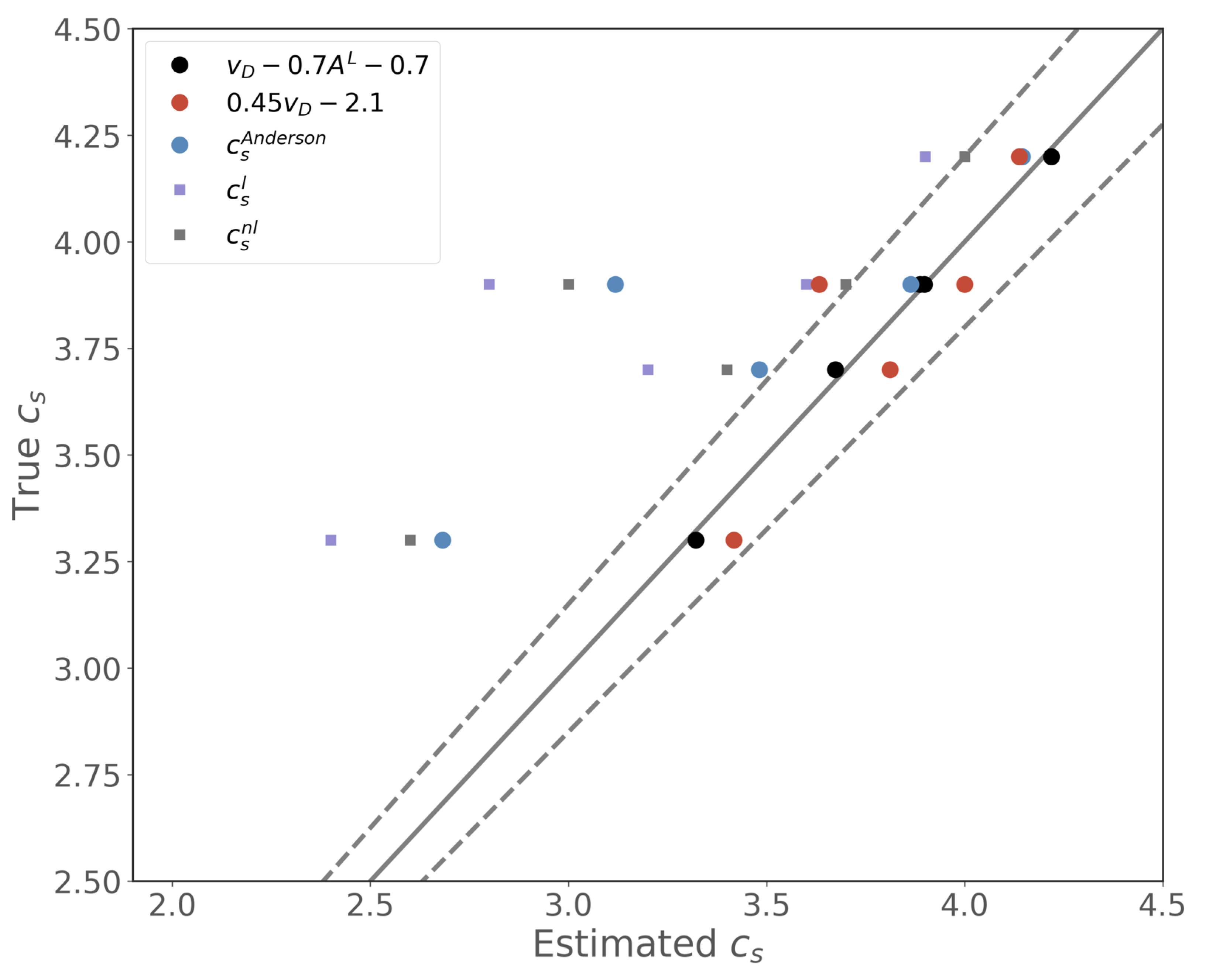
3.2. Extracting Seismic Wave Speeds

Section 2 and the previous subsection showed that the Debye speed extracted from the partial density of states (Equation (6)), is not equal to the Debye speed estimated from that material’s seismically observed wave speeds (Equation (3)). This result stems partly from the fact that the average of the inverse cube of a function (Equation (12)) is not generally equivalent to the inverse cube of the average (Equation (13)) and because seismic waves “see” the material’s isotropic properties in a specific manner. Therefore, the Debye speed estimated from seismic wave speeds is an upper bound for the material’s Debye speed $v_D$. This distinction is critical for geophysical applications of NRIXS, which typically seek to compare the experimentally observed Debye speed $v_{\widehat{\mathbf{k}}}$ or $v_D$ with seismically observed acoustic wave speeds $c_p$ and $c_s$. In this section, we focus on the issues associated with extracting seismic wave speeds based upon $v_D$.

A common procedure used to extract seismic wave speeds from NRIXS experiments is to use independent estimates of the the bulk modulus $\kappa$ and density $\rho$ from an equation of state based upon X-ray diffraction (e.g., [25,26,27,28,29,30]). For isotropic material, manipulating the expressions for the acoustic wave speeds (Equation (9) and noting that $\kappa ={\kappa }_0^V$ and $\mu ={\mu }_0^V$ in order to be compatible with the quantities provide by an Earth model such as PREM) combined with Equation (3) results in three equations for the three unknowns $\mu$, $c_p$, and $c_s$ in terms of the known quantities $v_D$, $\kappa$, and $\mu$ such that

$$\begin{array}{cc}\hfill \frac{\kappa }{\rho }& =c_p^2-\frac{4}{3}{c}_s^2,\hfill \\ \hfill \frac{\mu }{\rho }& =c_s^2,\mathrm{and}\hfill \\ \hfill \frac{1}{v_D^3}& =\frac{1}{3}\left(\frac{1}{c_p^3}+\frac{2}{c_s^3}\right).\hfill \end{array}$$

(21)

these equations are non-linearly dependent on $c_p$ and $c_s$, and are often solved by first linearizing the equations as is done in Equation (15) of Sturhahn & Jackson [3].

The form of the Debye speed (Equation (3)) used in Equation (21) is only applicable to isotropic materials, and significant errors may result when applied to anisotropic materials. The difference between the seismically relevant Debye speed $v_D^V$ (Equation (3)) and the observed Debye speed $v_D$ (Equation (7)) maps directly into the the estimated acoustic wave speeds, especially into shear wave speed, since the Debye speed is heavily weighted by the shear wave speed.

In order to estimate the magnitude of the errors associated with these approximations, acoustic wave speeds are estimated using the expressions in Equation (21) and the theoretical values of $v_D$, ${\kappa }_0^V$, and $\rho$ using the five hcp iron alloys in Table 1. Since the full elastic tensors for the materials are available, both the bulk modulus ${\kappa }_0^V$ and the Debye speed $v_D$ are calculated exactly. The inferred seismic wave speeds (

Table 3. Comparison of seismic wave speeds obtained from $v_D$ for iron alloys at inner core conditions (Table 1). The material’s true compressional wave speed ($c_p$; column 2) is compared against those obtained using linearized form of Equation (21) ($c_p^l$; column 3) and solving the full non-linear equations ($c_p^{nl}$; column 4). Columns 5 through 7 are the same as columns 2 through 4 except for shear waves. The last column gives the shear wave speed estimated from the Debye speed using the relationship of Anderson et al. [31] ($c_s^A$; Equation (22)).

Material	${\mathit{c}}_{\mathit{p}}$	${\mathit{c}}_{\mathit{p}}^{\mathit{l}}$	${\mathit{c}}_{\mathit{p}}^{\mathit{n}\mathit{l}}$	${\mathit{c}}_{\mathit{s}}$	${\mathit{c}}_{\mathit{s}}^{\mathit{l}}$	${\mathit{c}}_{\mathit{s}}^{\mathit{n}\mathit{l}}$	${\mathit{c}}_{\mathit{s}}^{\mathit{A}}$
hcp Fe	11.8	10.7 [–10%]	11.5 [–3%]	3.9	2.8 [–28%]	3.0 [–23%]	3.1 [–20%]
hcp Fe-Si	11.2	10.2 [–10%]	11.2 [–1%]	3.9	3.6 [–8%]	3.7 [–5%]	3.9 [–2%]
hcp Fe-Si-Ni	11.8	10.8 [–8%]	11.5 [–2%]	3.3	2.4 [–29%]	2.6 [–22%]	2.7 [–20%]
hcp Fe-Si-C	11.6	10.6 [–9%]	11.4 [–1%]	3.7	3.2 [–13%]	3.4 [–9%]	3.5 [–6%]
hcp Fe-S-C	11.8	10.6 [–10%]	11.7 [–1%]	4.2	3.9 [–7%]	4.0 [–5%]	4.1 [–1%]

) using the linear solution of Sturhahn & Jackson [3] show that the linear approximation results in errors in the compressional wave speed on the order of $10\%$ and errors in the shear wave speed of 10–30%. Therefore, for iron alloys relevant for the Earth’s inner core, linearization of Equation (21) results in significant errors due to the terms neglected when linearizing the set of equations. Solving the non-linear system of equations (Equation (21)) captures the compressional wave speed to within several percent, however, significant errors of $25\%$ in shear wave speed remain (Figure 4). The errors associated with these solutions are smaller than those of the linearized solutions, however, they are substantial, especially for the shear wave speed. The source of the error is the assumption that $v_D\approx v_D^V$, that is, relating $v_D$ directly to the seismic speeds even though the material is not isotropic (the third equation in Equation (21)).

Previous estimates of the error due to anisotropy in the seismic speeds obtained from the Debye speed are of the order of a few percent [32], while the errors in this study are found to be considerably larger (Table 3). Bosak et al. [32] significantly underestimates the error due to their choice of averaging scheme. They use an averaging scheme [33] which yields acoustic wave speeds that are similar to those obtained by the Voigt-Ruess-Hill average. However, when comparing with seismic wave speeds from a model such as PREM [13], the wave speeds should be calculated using the Voigt average [14].

Finally, Anderson [10] argued that the ratio $c_s/v_D$ is roughly a constant value of $0.9\pm 0.001$, and thus for isotropic materials, the Debye speed may be related to the shear wave speed as [31]

$$c_s\approx 0.9\times v_D.$$

(22)

Surprisingly, this simple estimate of $c_s$ (Table 3) out-performs all other estimates of $c_s$. Motivated by this result, we perform a simple regression against the strength of anisotropy and find that

$$c_s\approx 1.0\times v_D+0.7\times A^L-0.7,$$

(23)

where $c_s$ and $v_D$ are given in km/s. This relationship is able to provide a good fit to $c_s$ with less than one percent error (Figure 5). Unfortunately, the strength of anisotropy is not typically known, and in that case, the regression

$$c_s\approx 0.45\times v_D-2.1,$$

(24)

can predict the shear wave speed to within ∼$5\%$ (Figure 5).

The problem of estimating seismic wave speeds can be turned around to estimate Debye speeds based upon seismically constrained wave speeds. Consider, for illustrative purposes, the seismically observed isotropic wave speeds of the inner core from the PREM model ($c_p=11.1$ km/s and $c_s=3.6$ km/s; [13]). These isotropic values can be used to calculate Debye speed of $v_D=4.10$ km/s if the inner core is isotropic (Equation (3)). Alternatively, using the five elastic constants describing transversely isotropic inner core from seismological observations ($c_{11}=1577$ GPa, $c_{33}=1647$ GPa, $c_{13}=1259$ GPa, $c_{44}=168$ GPa, $c_{66}=151$ GPa; [14]), the Debye speed is $v_D=4.06$ km/s (Equation (2)). This value of the Debye speeds is most similar to that of the bcc iron alloy (4.04 km/s), and least similar to that of the hcp Fe-Si-Ni alloy (2.90 km/s; Table 2). However, comparison of the seismic wave speeds (Table 1) suggests the opposite result, with the hcp Fe-Si-Ni alloy ($c_p=11.8$ km/s and $c_s=3.3$ km/s) being more consistent with the seismically observed values than those of the bcc Fe-Si alloy ($c_p=11.5$ km/s and $c_s=4.2$ km/s). This is due to the fact that the higher strength of anisotropy of the bcc Fe-Si crystal lowers its Debye speed, hence the comparison of the Debye speed for anisotropic material ideally should be done with the strength of the anisotropy of the material.

4. Conclusions

The seismic wave speeds of materials at high pressure and high temperature are often estimated from the partial phonon density of states obtained from nuclear resonant inelastic scattering experiments. This manuscript demonstrates that the Debye speeds extracted from these experiments are not equivalent to the Debye speed estimated from that material’s seismic wave speeds. Assuming that the experimentally observed Debye speed is equal to that based upon isotropic seismic wave speeds introduces significant error for iron alloys at inner core conditions. The magnitude of these errors depends on the strength of anisotropy, and results in an error of ∼$20\%$ per unit of anisotropy. A second source of error arises when the approximate linearized solutions (i.e., Equations (15) of Sturhahn & Jackson [3]) are used to estimated compressional and shear wave speeds.

Furthermore, it is shown that the Debye speed estimated from the seismic wave speeds provides an upper bound to the true Debye speed. Consequently, the acoustic wave speeds extracted from the NRIXS experiments are underestimated compared to the true seismic wave speeds as obtained through seismological observations. The compressional wave speed $c_p$ is underestimated by ∼$10\%$ per unit of anisotropy, and the shear wave speed $c_s$ is underestimated by ∼$25\%$ per unit of anisotropy. Previous estimates of the error associated with anisotropy are underestimated due to the choice of an averaging scheme that is not the Voigt averaging scheme relevant for models based upon seismological observations. For iron alloys at inner core conditions, new empirical relationships are derived to estimate the seismic shear wave speed from the experimentally derived Debye speed within ∼$5\%$ error. Additionally, it is shown that if the strength of anisotropy is known, the accuracy of the estimated seismic wave speeds can be dramatically improved. The results in this study are crucial to constraining the inner core’s light element composition, and for determining the presence of partial melt.

References

1. Sturhahn, W. Nuclear resonant spectroscopy. Phys. Condens. Matter 2004, 416, S497–S530. [Google Scholar] [CrossRef]
2. Dauphas, N.; Hu, M.Y.; Baker, E.M.; Hu, J.; Tissot, F.L.; Alp, E.E.; Roskosz, M.; Zhao, J.; Bi, W.; Liu, J.; et al. SciPhon: A data analysis software for nuclear resonant inelastic X-ray scattering with applications to Fe, Kr, Sn, Eu and Dy. J. Synchrotron Radiat. 2018, 25, 1581–1599. [Google Scholar] [CrossRef] [PubMed] [Green Version]
3. Sturhahn, W.; Jackson, J.M. Geophysical Applications of Nuclear Resonant Spectroscopy; Ohtani, E., Ed.; Advances in High-Pressure Mineralogy; The Geological Society of America: Boulder, CO, USA, 2007; pp. 157–174. [Google Scholar]
4. Antonangeli, D.; Ohtani, E. Sound velocity of hcp-Fe at high pressure: Experimental constraints, extrapolations and comparison with seismic models. Prog. Earth Planet. Sci. 2015, 2, 3. [Google Scholar] [CrossRef]
5. Singwi, K.S.; Sjölander, A. Resonance absorption of nuclear gamma rays and the dynamics of atomic motions. Phys. Rev. 1960, 120, 1093–1102. [Google Scholar] [CrossRef]
6. Sturhahn, W.; Toellner, T.S.; Alp, E.E.; Zhang, X.; Ando, M.; Yoda, Y.; Kikuta, S.; Seto, M.; Kimball, C.W.; Dabrowski, B. Phonon density of states measured by inelastic nuclear resonant scattering. Phys. Rev. Lett. 1995, 74, 3832–3835. [Google Scholar] [CrossRef] [PubMed] [Green Version]
7. Chumakov, A.I.; Rüffer, R.; Baron, A.Q.R.; Grünsteudel, H.; Grünsteudel, H.F.; Kohn, V.G. Anisotropic inelastic nuclear absorption. Phys. Rev. B 1997, 56, 10758. [Google Scholar] [CrossRef]
8. Kohn, V.G.; Chumakov, A.I.; Rüffer, R. Nuclear resonant inelastic absorption of synchrotron radiation in an anisotropic single crystal. Phys. Rev. B 1998, 58, 8437–8444. [Google Scholar] [CrossRef]
9. Anderson, O.L. A simplified method for calculating the Debye temperature from elastic constants. J. Phys. Chem. Solids 1963, 24, 909–917. [Google Scholar] [CrossRef]
10. Anderson, O.L. An approximate method of estimating shear velocity from specific heat. J. Geophys. Res. Lett. 1965, 70, 4726–4728. [Google Scholar] [CrossRef]
11. Sturhahn, W.; Kohn, V. Theoretical aspects of incoherent nuclear resonant scattering. Hyperfine Interact. 1999, 123, 367–399. [Google Scholar] [CrossRef]
12. Hu, M.Y.; Sturhahn, W.; Toellner, T.S.; Mannheim, P.D.; Brown, D.E.; Zhao, J.; Alp, E.E. Measuring velocity of sound with nuclear resonant inelastic X-ray scattering. Phys. Rev. B 2003, 67, 094304. [Google Scholar] [CrossRef] [Green Version]
13. Dziewoński, A.M.; Anderson, D.L. Preliminary reference earth model. Phys. Earth Planet. Int. 1981, 25, 297–356. [Google Scholar]
14. Delbridge, B.G.; Ishii, M. Reconciling elasticity tensor constraints from mineral physics and seismological observations: Applications to the earth’s inner Core. Geophys. J. Int. 2019. submitted. [Google Scholar]
15. Jensen, J.L.W.V. Sur les fonctions convexes et les inegalites entre les valeurmoyennes. Acta Math. 1906, 30, 175–193. [Google Scholar] [CrossRef]
16. Roberts, A.W.; Varberg, D.E. Convex Functions; Academic Press: Cambridge, MA, USA, 1973. [Google Scholar]
17. Steinle-Neumann, G.; Stixrude, L.; Cohen, R.E.; Gülseren, O. Elasticity of iron at the temperature of the Earth’s inner core. Nature 2001, 413, 57–60. [Google Scholar] [CrossRef]
18. Tsuchiya, T.; Kuwayama, Y.; Ishii, M.; Kawai, K. High-P, T elasticity of iron-light element alloys[MR33E-05]. In Proceedings of the 2017 Fall Meeting, AGU, New Orleans, LA, USA, 11–15 December 2017. [Google Scholar]
19. Li, Y.; Vočadlo, L.; Brodholt, J.P. The elastic properties of hcp-Fe alloys under the conditions of the Earth’s inner core. Earth Planet. Sci. Lett. 2018, 493, 118–127. [Google Scholar] [CrossRef]
20. Martorell, B.; Wood, I.G.; Brodholt, J.; Vočaldo, L. The elastic properties of hcp-Fe1- xSix at Earth’s inner-core conditions. Earth Planet. Sci. Lett. 2016, 451, 89–96. [Google Scholar] [CrossRef] [Green Version]
21. Belonoshko, A.B.; Skorodumova, N.V.; Davis, S.; Osiptsov, A.N.; Rosengren, A.; Johansson, B. Origin of the low rigidity of the Earth’s inner core. Science 2007, 316, 1603–1605. [Google Scholar] [CrossRef]
22. Kube, C.M. Elastic anisotropy of crystals. AIP Adv. 2016, 6, 095209. [Google Scholar] [CrossRef]
23. Ranganathan, S.I.; Ostoja-Starzewski, M. Universal elastic anisotropy index. Phys.Rev. Lett. 2008, 101, 055504. [Google Scholar] [CrossRef] [Green Version]
24. Chung, D.H.; Buessem, W.R. The Elastic Anisotropy of Crystals. J. Appl. Phys. 1967, 38, 2010–2012. [Google Scholar] [CrossRef]
25. Mao, H.K.; Xu, J.; Struzhkin, V.V.; Shu, J.; Hemley, R.J.; Sturhahn, W.; Hu, M.Y.; Alp, E.E.; Vocadlo, L.; Alfè, D.; et al. Phonon density of states of iron up to 153 gigapascals. Science 2001, 292, 914–916. [Google Scholar] [CrossRef] [PubMed]
26. Lin, J.F.; Struzhkin, V.V.; Sturhahn, W.; Huang, E.; Zhao, J.; Hu, M.Y.; Alp, E.E.; Mao, H.K.; Boctor, N.; Hemley, R.J. Sound velocities of iron-nickel and iron-silicon alloys at high pressures. Geophys. Res. Lett. 2003, 30, 11. [Google Scholar] [CrossRef] [Green Version]
27. Jackson, J.M.; Hamecher, E.A.; Sturhahn, W. Nuclear resonant X-ray spectroscopy of (Mg, Fe) SiO3 orthoenstatites. Eur. J. Mineral. 2009, 21, 551–560. [Google Scholar] [CrossRef] [Green Version]
28. Prescher, C.; Dubrovinsky, L.; Bykova, E.; Kupenko, I.; Glazyrin, K.; Kantor, A.; McCammon, C.; Mookherjee, M.; Nakajima, Y.; Miyajima, N.; et al. High Poisson’s ratio of Earth’s inner core explained by carbon alloying. Nat. Geosci. 2015, 8, 220. [Google Scholar] [CrossRef]
29. Wicks, J.K.; Jackson, J.M.; Sturhahn, W.; Zhang, D. Sound velocity and density of magnesiowüstites: Implications for ultra low-velocity zone topography. Geophys. Res. Lett. 2017, 44, 2148–2158. [Google Scholar] [CrossRef]
30. Finkelstein, G.J.; Jackson, J.M.; Said, A.; Alatas, A.; Leu, B.M.; Sturhahn, W.; Toellner, T.S. Strongly anisotropic magnesiowüstite in Earth’s lower mantle. J. Geophys. Res. 2018, 123, 4740–4750. [Google Scholar] [CrossRef]
31. Anderson, O.L.; Dubrovinsky, L.; Saxena, S.K.; LeBihan, T. Experimental vibrational Grüneisen ratio values for ϵ-iron up to 330 GPa at 300 K. Geophys. Res. Lett. 2001, 28, 399–402. [Google Scholar] [CrossRef]
32. Bosak, A.; Krisch, M.; Chumakov, A.; Abrikosov, I.A.; Dubrovinsky, L. Possible artifacts in inferring seismic properties from X-ray data. Phys. Earth Planet. Int. 2016, 260, 14–19. [Google Scholar] [CrossRef]
33. Matthies, S.; Humbert, M. On the principle of a geometric mean of even-rank symmetric tensors for textured polycrystals. J. Appl. Crystallogr. 1995, 28, 254–266. [Google Scholar] [CrossRef]
34. Fedorov, I. Theory of Elastic Waves in Crystals; Plenum Press: New York, NY, USA, 1968. [Google Scholar]
35. Musgrave, M. Crystal Acoustics; Holden-Day Series in Mathematical Physics: San Francisco, CA, USA, 1970; pp. 75–76. [Google Scholar]
36. Dahlen, F.; Tromp, J. Theoretical Global Seismology; Princeton University Press: Princeton, NJ, USA, 1998. [Google Scholar]
37. Chapman, C. Fundamentals of Seismic Wave Propagation; Cambridge University Press: Cambridge, UK, 2004. [Google Scholar]
38. Takeuchi, H.; Saito, M. Seismic surface waves. Methods Comput. Phys. 1972, 11, 217–295. [Google Scholar]
39. Backus, G.E. Possible forms of seismic anisotropy of the uppermost mantle under oceans. J. Geophys. Res. 1965, 70, 3429–3439. [Google Scholar] [CrossRef]
40. Every, A.G. General closed-form expressions for acoustic waves in elastically anisotropic solids. Phys. Rev. B 1980, 22, 1746–1760. [Google Scholar] [CrossRef]
41. Tromp, J. Normal-mode splitting due to inner-core anisotropy. Geophys. J. Int. 1995, 121, 963–968. [Google Scholar] [CrossRef] [Green Version]
42. Watt, J.P.; Peselnick, L. Clarification of the Hashin-Shtrikman bounds on the effective elastic moduli of polycrystals with hexagonal, trigonal, and tetragonal symmetries. J. Appl. Phys. 1980, 51, 1525–1531. [Google Scholar] [CrossRef]
43. Every, A.G. General, closed-form expressions for acoustic waves in cubic crystals. Phys. Rev. Lett. 1979, 42, 1065–1068. [Google Scholar] [CrossRef]
44. Antonangeli, D.; Krisch, M.; Fiquet, G.; Farber, D.L.; Aracne, C.M.; Badro, J.; Occelli, F.; Requardt, H. Elasticity of cobalt at high pressure studied by inelastic X-ray scattering. Phys. Rev. Lett. 2004, 93, 215505. [Google Scholar] [CrossRef] [Green Version]
45. Antonangeli, D.; Krisch, M.; Fiquet, G.; Badro, J.; Farber, D.L.; Bossak, A.; Merkel, S. Aggregate and single-crystalline elasticity of hcp cobalt at high pressure. Phys. Rev. B 2005, 72, 134303. [Google Scholar] [CrossRef] [Green Version]
46. Choy, M.M.; Hellwege, K.H.; Hellwege, A.M. Elastic, Piezoelectric, Pyroelectric, Piezooptic, Electrooptic Constants, and Nonlinear Dielectric Susceptibilities of Crystals: Revised and Expanded Edition of Volumes III/1 and III/2(Vol. 11); Springer: New York, NY, USA, 1979. [Google Scholar]
47. Goncharov, A.F.; Crowhurst, J.; Zaug, J.M. Elastic and vibrational properties of cobalt to 120 GPa. Phys. Rev. Lett. 2004, 92, 115502. [Google Scholar] [CrossRef]
Figure 1. Orientation of incident photons and propagation direction for a hexagonal crystal.
Minerals 10 00331 g001
Figure 2. Percent variation of v k ^ as a function of the strength of anisotropy A L for the five hcp iron alloys (black circles) in Table 1. The dashed line represents a linear best fit to the data.
Minerals 10 00331 g002
Figure 3. Distribution of the deviation of the Debye speed obtained using acoustic wave speeds estimated using the Voigt (red), Reuss (blue), and Voigt-Reuss-Hill (grey) averaged elasic moduli with respect to the true Debye speed. One million randomly generated tensors of materials with hexagonal symmetry and identical seismic wave speeds are used.
Minerals 10 00331 g003
Figure 4. The dependence of the deviation of the Debye speed v D from that based upon the Voigt average, v D V , and the seismic speeds for the hcp iron alloys in Table 1 as a function of the strength of anisotropy A L . The semi-transparent grey circles represent the difference between v D (Equation (7)) and v D V (Equation (3)) for 10 6 randomly generated transversely isotropic elastic tensors with the same seismic wave speeds as those of pure iron (Table 1). The red circles correspond to the difference between v D and v D V for the five hcp iron alloys (Table 1) and the blue and purple circles denote the corresponding deviation in inferred acoustic longitudinal and transverse wave speeds, respectively (Table 3). The dashed lines represent linear best fits to the acoustic wave speed data.
Minerals 10 00331 g004
Figure 5. Comparison of c s against estimates of c s derived from the Debye speed. The solid grey line represents a one-to-one line. The dashed lines represent ± 5 % of the shear speed. Points to the left of the grey line underestimate c s where as points to the right overestimate c s .
Minerals 10 00331 g005