1. Introduction
Hyperbolic spaces (see
Section 2 for definitions) were introduced by Mikhail Gromov in the 1980s in the context of geometric group theory (see [
1,
2,
3,
4]). Classical Riemannian geometry states that negatively-curved spaces possess an interesting property known as geodesic stability. Namely, near-optimal paths (quasi-geodesics) remain in a neighborhood of the optimal path (geodesic). When Mario Bonk proved in 1996 that geodesic stability was, in fact, equivalent to Gromov hyperbolicity (see [
5]), the theory of hyperbolic spaces became a way to grasp the essence of negatively-curved spaces and to translate it to the simpler and more general setting of metric spaces. In this way, a simple concept led to a very rich general theory (see [
1,
2,
3,
4]) and, in particular, made hyperbolic spaces applicable to graphs. The theory has also been extensively used in discrete spaces like trees, the Cayley graphs of many finitely-generated groups and random graphs (see, e.g., [
6,
7,
8,
9]).
Hyperbolic spaces were initially applied to the study of automatic groups in the science of computation (see, e.g., [
10]); indeed, it was proven that hyperbolic groups are strongly geodesically automatic, i.e., there is an automatic structure on the group [
11]. The concept of hyperbolicity appears also in discrete mathematics, algorithms and networking [
12]. For example, it has been shown empirically in [
13] that the Internet topology embeds with better accuracy into a hyperbolic space than into a Euclidean space of comparable dimension (formal proofs that the distortion is related to the hyperbolicity can be found in [
14]); furthermore, it is evidenced that many real networks are hyperbolic (see, e.g., [
15,
16,
17,
18,
19]). Recently, among the practical network applications, hyperbolic spaces were used to study secure transmission of information on the Internet or the way viruses are spread through the network (see [
20,
21]); also to traffic flow and effective resistance of networks [
22,
23,
24].
In fact, there is a new and growing interest for graph theorists in the study of the mathematical properties of Gromov hyperbolic spaces. (see, for example, [
6,
7,
8,
9,
14,
18,
19,
20,
21,
25,
26,
27,
28,
29,
30,
31,
32,
33,
34,
35]).
Several researchers have shown interest in proving that the metrics used in geometric function theory are Gromov hyperbolic. For instance, the Kobayashi and Klein–Hilbert metrics are Gromov hyperbolic (under certain conditions on the domain of definition; see [
36,
37,
38]), the Gehring–Osgood
j-metric is Gromov hyperbolic but the Vuorinen
j-metric is not Gromov hyperbolic, except in the punctured space (see [
39]). Furthermore, in [
40], the hyperbolicity of the conformal modulus metric
and the related so-called Ferrand metric
have been studied. Gromov hyperbolicity of the Poincaré and the quasi-hyperbolic metrics is also the subject of [
34,
41,
42,
43,
44,
45,
46].
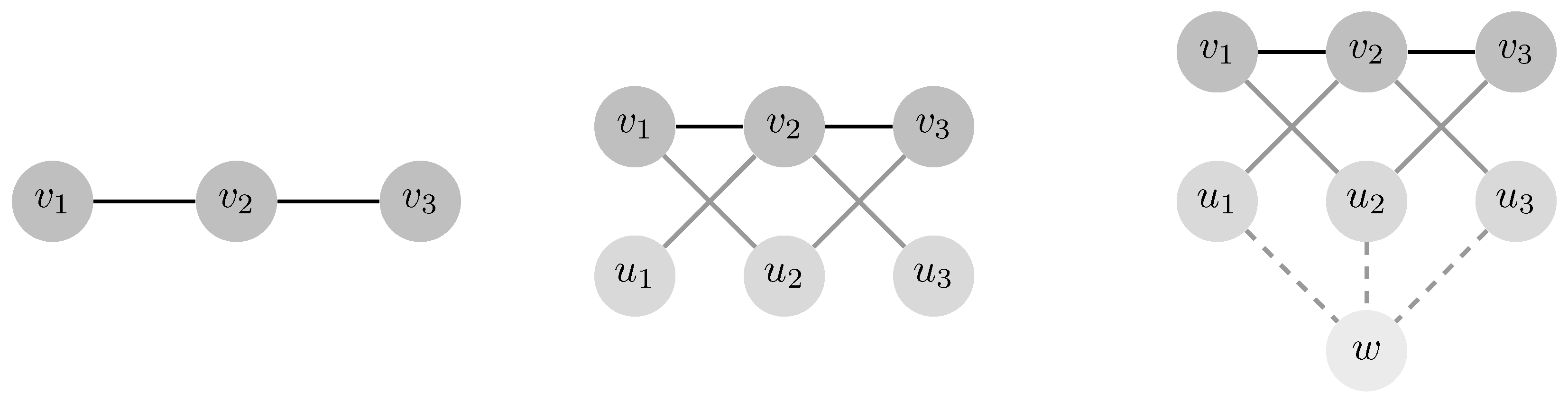
Mycielskian graphs (see
Section 2 for definitions) are a construction for embedding any undirected graph into a larger graph with higher chromatic number, but avoiding the creation of additional triangles. For example, the simple path graph with two vertices and one edge has chromatic number two, but its Mycielskian graph (which is the cycle graph with five vertices) raises that number to three. Actually, Jan Mycielski proved that there exist triangle-free graphs with an arbitrarily large chromatic number by applying this construction repeatedly to a starting triangle-free graph (see [
47]). This means that, on the one hand, this construction enlarges small graphs in order to increase their chromatic number, but on the other hand (as we prove in the present paper), the resulting graph is Gromov hyperbolic; furthermore, its hyperbolicity constant is strongly constrained to a small interval. In this work, we also characterize which graphs yield Mycielskian graphs with hyperbolicity constant in the boundary cases. Note that a constraint value of the hyperbolicity constant is relevant, since it gives an idea of the tree-likeness of the space in question (see [
35]).
Computing the hyperbolicity constant of a space is a difficult goal: For any arbitrary geodesic triangle
T, the minimum distance from any point
p of
T to the union of the other two sides of the triangle to which
p does not belong to must be calculated. Then, the hyperbolicity constant is the supremum over all the minimum distances of possible choices for
p and then over all of the possible choices for
T in that space. Anyhow, notice that in general, the main obstacle is locating the geodesics in the space. In [
2], the equivalence of the hyperbolicity of any geodesic metric space and the hyperbolicity of a graph associated with it are proven; similar results for Riemannian surfaces (with a very simple graph) can be found in [
34,
44,
45,
46]; hence, it is very useful to know hyperbolicity criteria for graphs. It is possible to compute the hyperbolicity constant of a finite graph with
n vertices in time
[
48] (this result is improved in [
17,
49]). There is an algorithm that allows to decide if a Cayley graph (of a presentation with a solvable word problem) is hyperbolic [
50]. However, there is no easy method to decide if a general infinite graph is hyperbolic or not.
Thus, a way to approach the problem is to study the hyperbolicity for particular types of graphs. For example, some other authors have obtained results on hyperbolicity for the complement of graphs, chordal graphs, vertex-symmetric graphs, lexicographic product graphs, corona and join of graphs, line graphs, bipartite and intersection graphs, bridged graphs, expanders and median graphs [
24,
27,
28,
32,
33,
35,
51,
52,
53,
54,
55,
56].
If
G is a graph,
denotes its Mycielskian graph (see
Section 2 for definitions), and
stands for its hyperbolicity constant. As usual, we denote by
and
as the set of vertices and edges of
G, respectively. Let us also denote by
the union of the set
and the midpoints of the edges of
G. The diameter of a graph
G (the maximum distance between any two points of
G) will be denoted by
and the diameter of the set of vertices
of
G by
.
The main results of this work deal with the hyperbolicity constant of Mycielskian graphs, as said above. The first of them states that Mycielskian graphs are always hyperbolic and solves the extremal problems of finding the smallest and largest hyperbolicity constants of such graphs. The second and third ones characterize graphs with hyperbolicity constants and , the maximum and the minimum values, respectively. The fourth result gives an accurate estimate of , and the fifth one allows us to obtain information on just in terms of .
Theorem 1. Let G be any graph. Then, is hyperbolic, and . Furthermore, if G is a complete graph, then ; otherwise:and both bounds of are sharp. Theorem 2. Let G be any graph. Then, if and only if there exists a geodesic triangle in G and with: Theorem 10 characterizes the graphs G with . Since this characterization is not easy to state briefly, we present here nice necessary and sufficient conditions on G for .
Theorem 3. Let G be any graph:Furthermore, the converses of (4) and (5) do not hold. The hyperbolicity of a metric space is at most half of its diameter. The following result states an unexpected fact: is not only upper bounded by ; in this case, that upper bound is close to the actual value of the hyperbolicity constant.
Theorem 4. Let G be any graph. Then: So far, our main results have obtained information about in terms of G. However, it is also interesting to consider what can be said about in terms of . Our next theorem gives a partial answer to this question.
Theorem 5. If , then .
The outline of the paper will be as follows. In
Section 2, some definitions and previous results will be stated.
Section 3 contains the proof of the main parts of Theorem 1.
Section 4 and
Section 5 will present the proofs of Theorem 2 and Theorem 3, respectively. In
Section 6, the hyperbolicity constants of the Mycielskian of path, cycle, complete and complete bipartite graphs are calculated explicitly. Apart from the intrinsic interest of these results, they are also employed in the proofs of some of the main results of the paper. Furthermore, it contains the proofs of Theorems 1, 4 and 5. Finally, in
Section 7, a characterization for graphs with
is given.
Since the hypotheses in most theorems are simple to check, the main results in this paper can be applied to every graph. An exception is Theorem 10, but even in this case, a rough algorithm is provided, which allows one to check the hypotheses in polynomial time. Furthermore, information on
from
G and on
in terms of
is found. The main inequalities obtained in this work are applied in
Section 6 in order to compute explicitly the hyperbolicity constants of the Mycielskian of some classical examples, such as path, cycle, complete and complete bipartite graphs. Finally, note that Mycielskian graphs are not difficult to identify computationally.
2. Definitions and Background
If
is a continuous curve in a metric space
, we can define the length of
as:
The curve
is a geodesic if we have
for every
(then
is equipped with an arc-length parametrization). The metric space
X is said to be geodesic if for every couple of points in
X, there exists a geodesic joining them; we denote by
any geodesic joining
x and
y; this notation is ambiguous, since in general we do not have the uniqueness of geodesics, but it is very convenient. Consequently, any geodesic metric space is connected. The graph
G consists of a collection of vertices, denoted by
and a collection of edges joining vertices,
; the edge joining vertices
and
will be denoted by
. Furthermore,
will stand for the set of neighbors of (or adjacent to) the vertex
, that is the set of all vertices
for which
. All throughout this paper, the metric space
X considered is a graph with every edge of length one. In order to consider a graph
G as a geodesic metric space, we identify (by an isometry) any edge
with the interval
in the real line. Thus, the points in Gare the vertices and the points in the interiors of the edges of G. In this way, any connected graph
G has a natural distance defined on its points, induced by taking the shortest paths in
G, and we can see
G as a metric graph. Such a distance will be denoted by
. Throughout this paper,
G denotes a connected (finite or infinite) simple (i.e., without loops and multiple edges) graph such that every edge has length one and
. These properties guarantee that
G is a geodesic metric space and that
can be defined. Note that excluding multiple edges and loops is not an important loss of generality, since ([
57], Theorems 8 and 10) they reduce the problem of computing the hyperbolicity constant of graphs with multiple edges and/or loops to the study of simple graphs.
A cycle in G is a simple closed curve containing adjacent vertices . It will be denoted by . The notation means that the vertices a and b are adjacent.
Given a graph
G with
, the Mycielskian graph
of
G contains
G itself as a subgraph, together with
additional vertices
, where each vertex
is the mirror of the vertex
of
G and
w is the supervertex. Each vertex
is connected by an edge to
w. In addition, for each edge
of
G, the Mycielskian graph includes two edges,
and
(in
Figure 1, the process of the construction of the Mycielskian graph for the path graph
is shown). Thus, if
G has
n vertices and
m edges, then
has
vertices and
edges.
Trivially, for all , and ; also and for any point , . Note that a can be either a vertex of the graph or any other point belonging to an edge of it. Moreover, the definition of makes sense also if , i.e., if G is an infinite graph. Since is always connected, it would be possible to consider disconnected graphs G, but Theorem 9 shows that, in order to study , it suffices to consider just connected graphs.
Finally, let us recall the definition of Gromov hyperbolicity that we will use (we use the notations of [
3]).
If
X is a geodesic metric space and
, the union of three geodesics
,
and
is a geodesic triangle that will be denoted by
, and we will say that
and
are the vertices of
T; it is usual to write also
. We say that
T is
-thin if any side of
T is contained in the
-neighborhood of the union of the two other sides. We denote by
the sharp thin constant of
T, i.e.,
Given a constant
, the space
X is
-hyperbolic if every geodesic triangle in
X is
-thin. We denote by
the sharp hyperbolicity constant of
X, i.e.,
We say that
X is hyperbolic if
X is
-hyperbolic for some constant
, i.e.,
. If we have a geodesic triangle with two identical vertices, we call it a bigon. Obviously, every bigon in a
-hyperbolic space is
-thin. In the classical references on this subject (see, e.g., [
2,
3]) appear several different definitions of Gromov hyperbolicity, which are equivalent in the sense that if
X is
-hyperbolic with respect to one definition, then it is
-hyperbolic with respect to another definition (for some
related to
). We have chosen this definition by its deep geometric meaning [
3].
Trivially, any bounded metric space
X is
-hyperbolic. A normed real linear space is hyperbolic if and only if it has dimension one. A geodesic space is zero-hyperbolic if and only if it is a metric tree. The hyperbolic plane (with curvature
) is
-hyperbolic. Every simply-connected complete Riemannian manifold with sectional curvature verifying
, for some positive constant
k, is hyperbolic. See the classical [
1,
3] in order to find more examples and further results.
Trees are one of the main examples of hyperbolic graphs. Metric trees are precisely those spaces
X with
. Therefore, the hyperbolicity constant of a geodesic metric space can be seen as a measure of how “tree-like” that space is. This alternative view of the hyperbolicity constant is an interesting subject since the tractability of a problem in many applications is related to the tree-like degree of the space under investigation. (see, e.g., [
58]). Furthermore, it is well known that any Gromov hyperbolic space with
n points embeds into a tree metric with distortion
(see, e.g., [
3], p. 33).
If and are isomorphic, we write . It is clear that if , then .
The following well-known result will be used throughout the paper (see, e.g., ([
59], Theorem 8) for a proof).
Lemma 1. Let G be any graph. Then, .
Consider the set of geodesic triangles T in G that are cycles and such that the three vertices of the triangle T belong to , and denote by the infimum of the constants such that every triangle in is -thin.
The following results, which appear in [
60] (Theorems 2.5, 2.7 and 2.6), will be used throughout the paper.
Lemma 2. For every graph G, we have .
Lemma 3. For any hyperbolic graph G, there exists a geodesic triangle such that .
The next result will narrow the possible values for the hyperbolicity constant .
Lemma 4. Let G be any graph. Then, is always a multiple of .
The following results deal with isometric subgraphs and how the hyperbolicity constant behaves.
A subgraph
of the graph
G is an isometric subgraph if for all
, we have
. This is equivalent to the fact that
for every
. It is known that isometric subgraphs have a lesser hyperbolicity constant (see [
57], Lemma 7):
Lemma 5. Let be an isometric subgraph of G. Then, .
The coming lemma states that the Mycielskians preserve isometric subgraphs, and a nice corollary follows.
Lemma 6. If is an isometric subgraph of G, then is an isometric subgraph of .
Proof. Let . Throughout the proof, , and with w being the supervertex.
Without loss of generality, or and . Otherwise, trivially, if or if and , then ; also trivially, if and , then .
First, let and . If , trivially, .
If , there exists so that . Notice also that . Suppose there is a path from to such that ; then, , and thus, , giving , which contradicts .
Additionally, if , then there is a geodesic path in and with and . Clearly, . By the triangle inequality, . Suppose there is a path from to such that , then , and there exists with ; thus, , giving , which is a contradiction.
Next, let and . Notice that . If , then the result trivially holds. If , then there exists with and , and thus, . Finally, if , then there is a geodesic both in an , which contains w. ☐
This result has a straightforward consequence.
Corollary 1. If is an isometric subgraph of G, then .
Denote by the subgraph of induced by . The following result is elementary.
Proposition 1. Let G be any graph. Then, G is an isometric subgraph of .
Proof. Consider the vertices and a geodesic in from to , say, with or , and . It suffices to find a curve in G from to with . Since, by construction, if , then , we have that joins and with . ☐
3. Proof of the Main Parts of Theorem 1
In order to prove the main parts of Theorem 1, consider first the following weaker version:
Theorem 6. Let G be any graph. Then, is hyperbolic, , and: Proof. For the upper bounds, notice that for any two vertices , , therefore , , and thus, by Lemma 1.
For the lower bounds, recall that for every , and thus, . If and p is the midpoint of , then and .
For , observe that, since , there exists , and thus, always contains a cycle of length of five, namely . Let x be the midpoint of and consider the geodesic bigon with geodesics and . If p is the midpoint of the geodesic , then one gets . ☐
The following lemmas relate with for small diameters.
Lemma 7. Let G be any graph. Then:
- (i)
If and , then .
- (ii)
If and , then .
Proof. Since G is a subgraph of , we have .
Assume that and , and let be a geodesic in G. Define (respectively, ) as the closest vertex to x (respectively, y) from (it is possible to have and/or ). Since is an integer number and by hypothesis, we have that:
Seeking for a contradiction, assume that . Thus, there exists a geodesic joining x and y in with , and by Proposition 1. Define (respectively, ) as the closest vertex to x (respectively, y) from .
Since
or
holds, we have
. Since
,
and:
which is a contradiction. Then,
and
holds.
Assume now that
and
. If
, then
gives the result. If
, then
. The argument in the proof of
gives:
and:
Therefore,
holds. ☐
Lemma 8. Let G be any graph. Then: Proof. Assume first that .
Let . Thus:
If , then clearly , and by Lemma 7, we conclude .
If , then .
If and , then and (if ).
If , then .
Therefore, .
For the other direction, let be so that . By Lemma 7, we have , and thus, .
Assume now that . Theorem 6 gives , and then, . ☐
We can prove now the main parts of Theorem 1.
Theorem 7. Let G be any graph. Then, is hyperbolic, and . Furthermore, if G is not a complete graph, then: Proof. Theorem 6 proves all of the statements of Theorem 7 except for the upper bound for in the case where .
However, if , then either , in which case G would be isomorphic to a complete graph, or , in which case , where the last equality follows from the above result, Lemma 8. ☐
As a consequence of Lemma 8, we obtain the following result.
Corollary 2. If G is not a complete graph, then .
The following result provides information about in terms of .
Theorem 8. Let G be any graph. If , then .
Proof. By Lemma 3, there is a geodesic triangle in G (with geodesics joining and in G) and with and . If , then is also a geodesic in by Lemma 7. If , then and ; hence, Lemma 7 gives that is a geodesic in . Therefore, T is also a geodesic triangle in . Since , then by Lemma 7. ☐
We say that a vertex v of a (connected) graph is a cut-vertex if is not connected. A graph is bi-connected if it does not contain cut-vertices. Given any edge in , we consider the maximal bi-connected subgraph containing it.
Finally, we have the following result regarding disconnected graphs. Even though in order to study Gromov hyperbolicity, connected graphs are needed, since is always connected, the original graph G does not need to be:
Theorem 9. Let G be any disconnected graph with connected components . Then: Proof. It is well known that the hyperbolicity constant of a graph is the maximum value of the hyperbolicity constant of its maximal bi-connected components. Since G is not connected, the supervertex is the unique cut-vertex in , and the subgraphs are the maximal bi-connected components of . Hence, the equality holds. ☐
Note that, in order to study , it suffices to consider just (connected) graphs G by Theorem 9.
4. Proof of Theorem 2
The next lemma will be a key tool:
Lemma 9. Let G be any graph. If , is a geodesic triangle in , such that and with , then , , and .
Proof. Since , and , , then by Theorem 6. Thus, . The equality and the fact that , guarantee that . In fact, for otherwise , and since , the triangle inequality would give . Therefore, . This in turn implies that . ☐
When comparing hyperbolicity constants of G and , it is useful to compare triangles in those graphs. A useful tool will be a projection, which allows one to associate triangles with given triangles , which do not contain the supervertex, that is . Namely:
Definition 1. The projection is defined as follows:
For a point , if , then . If , then . If , then a lies on an edge, say ; then, , so that .
Remark 1. Observe the following:
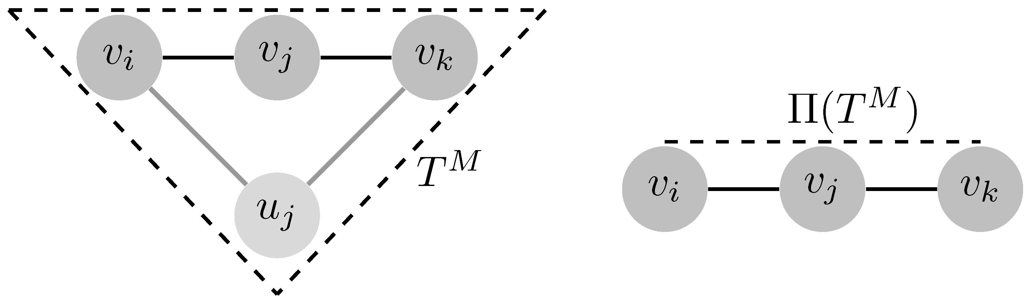
If is a geodesic in and , there exists a geodesic ; in general, equality does not hold, since two different edges in γ might project onto the same edge in (for instance, if , then ; note that ); therefore, .
If and , then .
If is a geodesic triangle in and is a geodesic triangle in G and , then does not need to be a cycle even if is. For instance, if and , then is a geodesic bigon in , are geodesics in G, but is not a cycle, although is; note that (see Figure 2).
However, the following holds:
Lemma 10. Let G be any graph and Π the projection in Definition 1. If and , then is a geodesic in G joining and . Furthermore, if , then .
Proof. The statement is trivial if . Otherwise, it is a consequence of the following fact: If , then we have either or for some and . If , then ; if , then . ☐
Proof of Theorem 2. Assume first that .
By Lemma 3, there is a geodesic triangle that is a cycle with and , so that . Then, by Lemma 9, , , p is the midpoint in , and .
The goal is to produce a triangle T from this , which is geodesic both in G and .
To this end, it will be first shown that the supervertex .
Clearly, for , since for all . For this same reason, , for , since . Finally, , since and , gives , which would mean that , which is a contradiction.
Therefore, , , and , and .
If we define
,
,
, then (
1) stated in Theorem 2 holds, and Lemma 7 gives
,
,
. If
and
, then
,
and
are geodesics in
G by Lemma 10. Otherwise,
or
have length at most two. By symmetry, we can assume that
; since
, we have
, and Lemma 10 gives that
and
are geodesics in
G. Furthermore,
contains a geodesic
in
G. This gives the existence of the geodesic triangle
T of Theorem 2 and (
2) stated in this same Theorem.
Next, let us show that . If , then , and the statement trivially holds. Assume that (thus, ). Since and , Lemma 10 gives that . Since , we have , and we conclude .
Let be a geodesic joining and in with , and let , so that is adjacent to (so ). We have .
If , then , and take to be the curve (not necessarily geodesic) ; then , and we conclude , the desired result.
If , let so that is adjacent to . Notice that cannot be the supervertex, for then , and it would not be a geodesic; thus, . Moreover, since and . Since , one gets , and we conclude .
Therefore, . Thus, in order to finish the proof of , one must show that .
Since is a geodesic triangle in G and , . Let us show that , thus finishing the proof.
Let . Seeking for a contradiction, assume , then, in fact, and .
If , then . Since and , we have . Let be the mirror vertex of p. Since , then . There is , with , and so, , a contradiction.
If and satisfies , then and v are adjacent. Let u be a vertex with and ; so , which is a contradiction.
Finally, if , then the vertex , which gives the minimum distance to p, either belongs to the mirror vertices or to G, but in any case, it is adjacent to an adjacent vertex of p; thus, , which is a contradiction.
In summary, .
Let us show the other implication to conclude that .
By Theorem 6, .
Let
be the geodesic triangle in
G in the hypothesis. Properties (
1) and (
2) stated in Theorem 2 and Lemma 7 give that
T is also a geodesic triangle in
. Since
, Lemma 7 gives
, finishing the proof. ☐
The proof of Theorem 2 has the following consequence.
Corollary 3. If the geodesic triangle T in G satisfies (1), (2) and (3) stated in Theorem 2, then T is also a geodesic triangle in . We also have the following corollaries of Theorem 2.
Corollary 4. If G is a graph with and , then .
Corollary 5. If G is a graph such that it does not contain a cycle σ satisfying , then: Remark 2. If G contains a cycle σ with , one cannot say anything more precise about apart from the bounds obtained in Theorem 6, which are applicable to all Mycielskian graphs, i.e., . In the particular case when G is the cycle graph , with , then Proposition 4 gives ; and if G is the complete graph , with , then by Proposition 5.
Given a graph
G, we define its circumference as:
Proposition 2. If G is a graph with , then: Proof. By Corollary 5, it suffices to show . By Lemma 3, there is a geodesic triangle T in G that is a cycle with . Since , if , then and by Lemma 7. Therefore, T is a geodesic triangle in and . ☐
Remark 3. If , one cannot say anything more precise about apart from the bounds obtained in Theorem 6, which are applicable to all Mycielskian graphs, i.e., . In particular, if , with , and G is the graph obtained from and by identifying the vertices and , then Corollary 1, Theorem 6 and Proposition 4 give and ; if G is the complete graph , with , then by Proposition 5.
5. Proof of Theorem 3
Proof. Assume first that . In order to prove , it will be enough to show that , by Lemma 1.
Note that since , then . Consider . If x or y is a vertex, then . Without loss of generality, . Note that for every and , since .
Trivially, for , or , or and , one gets .
When and , since for all vertices v in G, we have .
Assume that . Let , be so that x and y are the midpoints of the edges and , respectively. It is enough to consider the case where and . Since , we have ; since , we deduce , and then, . Thus, .
Finally, consider
and
. Let
so that
, and let
for some
u vertex in the mirror of
G. Since
,
, and thus,
. By symmetry, one can assume that
, and so,
and
. This gives the statement (
4).
Next, let us show that
implies
, proving statement (
5) of the Theorem. To this end, we shall construct a geodesic bigon with sides of length three.
Let be so that . If , then , and Proposition 3 and Corollary 6 give (of course, Theorem 3 is not used in the proofs of Proposition 3 and Corollary 6). Therefore, one can assume that .
Let with and ; note that . By symmetry, we can assume that . Let with and . Consider the geodesic bigon where , and . Therefore, taking , , and thus, .
This finishes the proof of both statements.
To show that the converse of (
4) does not hold, consider the graph
G with four vertices
and edges
,
. Then,
and
, where the only two points
that realize the diameter are
and
. Consider the geodesic bigon
given by
and
; let
be so that
. Then,
, and this bigon has
.
Since , we have . Notice that in order to have a geodesic triangle T with , one of its sides must have length three and, therefore, must have as its endpoints. As in the case of the bigon above, for any of these triangles, every vertex in is at a distance at most one of the other two sides. Therefore, all of these triangles satisfy . Therefore, .
Proposition 4 gives
. Since
, the converse of (
5) does not hold. ☐
6. Hyperbolicity Constant for Some Particular Mycielskian Graphs and the Proof of Theorems 1, 4 and 5
Computing the hyperbolicity constant of some graphs turns out to be specially useful. Namely, many graphs contain path graphs as isomorphic subgraphs; the cycle graph appeared naturally as a boundary situation for hyperbolicity constant of ; and finally, graphs isomorphic to the complete one were of interest. In this section, the precise hyperbolicity constants of the Mycielskian graphs for such graphs is calculated.
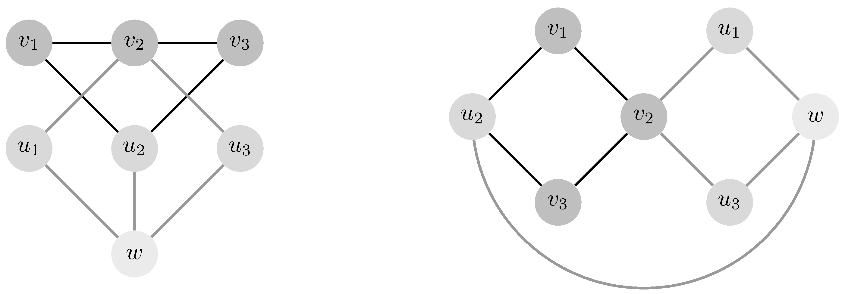
Proposition 3. Let be the path graph with n vertices. Then: Proof. Denote by
the vertices of
with
for
. One can easily check that
(see
Figure 3). Since
, Lemma 1 gives
for
. Then, Theorem 6 let us get the desired result for
.
For and , a similar argument will be used. First, a triangle T with the desired will be constructed, giving the lower bound; then, the diameter of the Mycielskian will give the upper bound.
In , consider the triangle , where , , , and take p as the midpoint of . Here, . One can check that . Therefore, Lemma 1 gives .
A similar argument works for .
A simple argument will give the result for .
For
, Theorems 2, 6 and Lemma 4 give
. Consider the geodesic triangle
with
,
y the midpoint in
and
, and take
p the midpoint in
(see
Figure 4). Then,
, since
.
All that is left is to prove that , which will automatically imply as well by Corollary 1, since .
By Lemma 3, let
be a geodesic triangle, so that
, and let
be so that
. Seeking for a contradiction, assume that
. This would mean
by Lemma 4 and Theorem 6. However, by Theorem 2,
, since every geodesic triangle in
has a hyperbolicity constant equal to zero, like any geodesic triangle in any tree. That is:
Some observations:
for otherwise
(via
w), contradicting (
9). Moreover, without loss of generality, we can assume that
always and
if
and
if
. Last,
for otherwise
T would be a cycle of diameter two, and thus,
.
Suppose that
. By (
8) and (
9),
. It is easy to check that
. Thus, we deduce
.
Since
, we have
. Since
, (
8) and (
9) give
. By symmetry, we can assume that
x is the midpoint of either
or
. Assume that
(the case
is similar). Since
T is a cycle and
, we have
,
and
. Then,
, a contradiction. Hence,
.
A similar argument shows that , which contradicts the fact that . One concludes that , which together with the fact that gives the desired result. ☐
Remark 4. There are several definitions of Gromov hyperbolicity. They are all equivalent in the sense that if X is δ-hyperbolic with respect to the definition A, then it is -hyperbolic with respect to the definition B, for some (see, e.g., [2,3]). The definition that we have chosen in the present paper is known as the Rips condition. We decided to select it among others due to its deep geometric meaning (see, e.g., [3]). As an example, the simplest existing proof of the invariance of hyperbolicity by quasi-isometries uses the Rips condition (see [3]) and so does the proof for geodesic stability (see [5]). Furthermore, some results that employ a different definition (such as the four-point condition) also require the Rips condition in their proofs (see, e.g., [27]). The Rips condition also comes up in a natural way when graphs with arbitrarily large edges are considered. Experience has shown that, although the definitions of hyperbolicity are equivalent, the values of the hyperbolicity constants of a space obtained when different definitions are considered have different behaviors actually.
As an example, the analogue of Proposition 3 for the hyperbolicity constant obtained applying the four-point condition (that we shall denote by ) says that and for every .
The following corollary is straightforward, but it is presented here because it is used to simplify the arguments in some other proofs in the paper.
Corollary 6. Let G be any graph. Then, .
Observe that this follows from Corollary 1, since if , then there exists a geodesic joining two vertices with length r. That is, is isomorphic to , and besides, is an isometric subgraph.
Proposition 3 and Corollaries 5 and 6 have the following consequence.
Corollary 7. If G is a graph with such that it does not contain a cycle σ satisfying , then .
By Lemmas 1 and 8, Proposition 3 and Corollary 6, we obtain the following result.
Corollary 8. Let G be any graph. Then:
- (i)
If , then .
- (ii)
If , then .
The next proposition deals with cycle graphs, which illustrate well the result of Theorem 2.
Proposition 4. Let be the cycle graph with n vertices. Then: Proof. Denote by the vertices of with edges . With the usual notation, is the mirror vertex of , and w is the supervertex.
For , and thus, . On the other hand, Theorem 6 gives .
For , , giving as an upper bound for the hyperbolicity constant. On the other hand, consider the bigon with x the midpoint of and y the midpoint of . Denote by the geodesic in T with ; thus, .
For , ; thus, the upper bound is . Consider the bigon T of antipodal vertices x, y in , with . Let p be the midpoint of ; then, and thus , which together with the upper bound, gives .
The range automatically follows from Theorem 2.
Finally, if , then , and Corollary 7 gives the result. ☐
Remark 5. The analogue of Proposition 4 for the hyperbolicity constant of the four-point condition says that for , , for and for every .
The complete graph has a very constant behavior.
Proposition 5. Let be the complete graph with n vertices. Then: Proof. Since and , by Propositions 3 and 4, one gets the result if .
For , Theorem 6 already gives , so it suffices to estimate the diameter of .
Notice . Without loss of generality, take ; clearly, if , then with equality if and ; if , then with equality if .
Summing up, ; thus, , which together with Theorem 6 prove the result. ☐
Remark 6. The analogue of Proposition 5 for the hyperbolicity constant of the four-point condition says that and for every .
The argument in the proof of Proposition 5 also gives the following result.
Corollary 9. If , then .
We can now finish the proof of Theorem 1.
Proof of Theorem 1: The main part follows from Theorem 7 for non-complete graphs. If G is a complete graph, Proposition 5 gives that
For the sharpness of , consider the graphs and , where stands for the path graph of vertices and edges , , and is the the cyclic graph with 10 vertices. From Propositions 3 and 4, we get and . ☐
Proof of Theorem 4. Lemma 1 gives the upper bound. If , then Theorem 6 gives . If , then Theorem 6 gives . Therefore, G is not a complete graph by Proposition 5. Thus, Theorem 8, Proposition 3 and Corollary 6 give . Hence, if , then we have by Proposition 3. If , then we have by Proposition 3. ☐
Proof of Theorem 5. By Theorem 4, we have . One can check that , and Theorem 8 gives . ☐
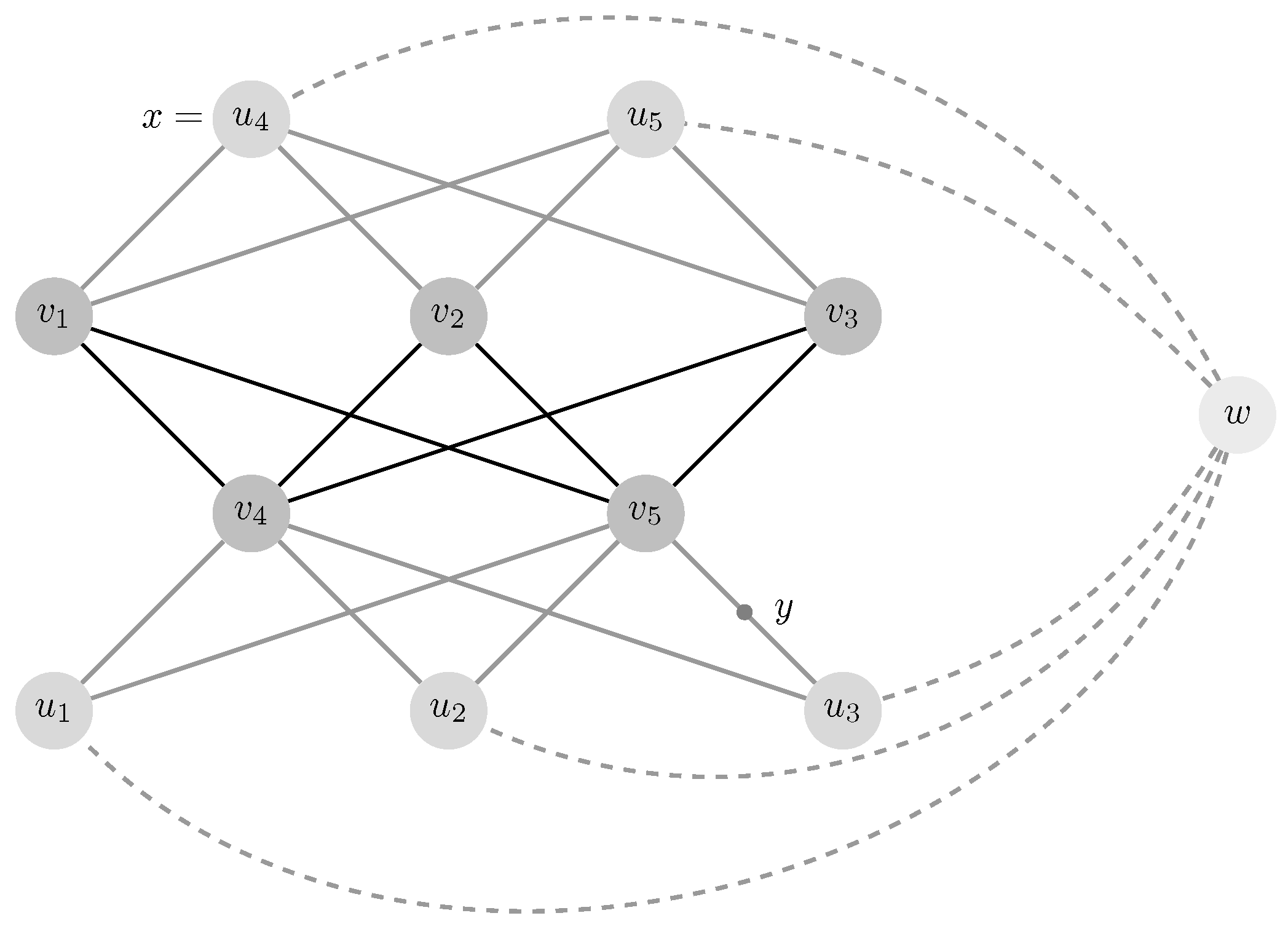
Proposition 6. Let be the complete bipartite graph with vertices. Then: Proof. As in the proof of Proposition 5, it suffices to show that .
One can check that
, and for every
, we have
(see
Figure 5); then,
. ☐
7. The Case of 5/4
In order to characterize the Mycielskian graphs with hyperbolicity constant , we define some families of graphs.
Denote by
the cycle graph with
vertices and by
the set of their vertices, such that
and
for
. Let
be the set of graphs obtained from
by adding a (proper or not) subset of the set of edges
,
. Let us define the set of graphs:
Let
be the set of graphs obtained from
by adding a (proper or not) subset of the set of edges
,
,
,
. Define:
Let
be the set of graphs obtained from
by adding a (proper or not) subset of the set
,
,
,
. Furthermore, let
be the set of graphs obtained from
by adding a (proper or not) subset of
,
,
,
. Define:
Let
be the set of graphs obtained from
by adding a (proper or not) subset of the set of edges
,
,
,
. Define:
Finally, we define the set
by:
In [
53] (Lemma 3.21) appears the following result.
Lemma 11. Let G be any graph. Then, if and only if there is a geodesic triangle in G that is a cycle with , and for some .
Finally, we obtain a simple characterization of the Mycielskian graphs with hyperbolicity constant .
Theorem 10. Let G be any graph. Then, if and only if and .
Proof. If , then . If , then Proposition 3 and Corollary 6 give .
Assume now and .
If , then G is a complete graph, and Proposition 5 gives .
If , then Lemma 8 gives , and thus, .
If , then Lemma 1 gives , and we conclude by Theorem 1.
If , then by Lemma 1. Besides, by Theorem 1. Hence, Lemma 4 implies . Seeking for a contradiction, assume that . By Lemma 3, there exists a geodesic triangle that is a cycle with and for some . Then, and . Since and T is a cycle, we have , . Since , , p is the midpoint of , and it is a vertex of . Thus, Lemma 11 gives , which is the contradiction we were looking for. Hence, , and we conclude . ☐
We finish this work with a computational remark about Theorem 10.
Let us consider a graph with m edges, a vertex with degree and the other vertices with degree at most . By choosing an edge , an edge ,..., and an edge , we can obtain the set of all paths of length in time ; hence, we can compute all cycles with length a in time . Therefore, it is possible to find a subgraph isomorphic to a fixed graph in (or in ) in time . Note that there are 4, 16, 16, 16 and 16 graphs in , , , and , respectively. Hence, we can find every subgraph of isomorphic to a graph in in time .
If G is a graph with n vertices, m edges and maximum degree , then is a graph with edges, a vertex with degree n and the other vertices with degree at most . Since , we can know if either or in time . Hence, to check the hypothesis is a tractable problem from a computational viewpoint, by using the algorithm sketched before.


