Fuel Consumption Estimation System and Method with Lower Cost

Abstract

This study proposes a fuel consumption estimation system and method with lower cost. On-board units can report vehicle speed, and user devices can send fuel information to a data analysis server. Then the data analysis server can use the proposed fuel consumption estimation method to estimate the fuel consumption based on driver behaviours without fuel sensors for cost savings. The proposed fuel consumption estimation method is designed based on a genetic algorithm which can generate gene sequences and use crossover and mutation for retrieving an adaptable gene sequence. The adaptable gene sequence can be applied as the set of fuel consumption in accordance with the pattern of driver behaviour. The practical experimental results indicated that the accuracy of the proposed fuel consumption estimation method was about 95.87%.

1. Introduction

With the development of the economic environment and the evolution of mobile communications, the intelligent transportation system has been more and more popular for obtaining fleet management services for the logistics industries and bus carriers [1]. A logistics company may have hundreds or thousands of trucks to provide freight services. However, the fuel cost of these industries is the most important challenge of fleet management services. For instance, Taiwan Institute of Economic Research (TIER) reported that the fuel costs of logistics industries and bus carriers were about 35.8 billion dollars [2] and 3.4 billion dollars [3], respectively, in Taiwan in 2015. Therefore, monitoring and saving fuel consumption efficiently can improve the profits for the logistics industries and bus carriers and reduce the air pollution from carbon dioxide (i.e., CO₂) for city governance [4,5].

For the measurement of fuel consumption, some studies used fuel sensors to detect the remaining quantity of fuel and calculated the differences among the remaining quantities. Furthermore, the data from the on-board diagnostics (OBD) could also be retrieved to obtain the fuel system status, vehicle speed, and engine revolutions per minute (RPM) [6,7,8,9]. Although these methods can measure the fuel consumption, fuel sensors and OBD devices should be equipped to report the fuel quantity data periodically, albeit with higher cost. For instance, the cost of a fuel level sensor is about 150,000 dollars, and the cost of data communications is about 13,000 dollars per month in Taiwan for a fleet of 1000 vehicles. Moreover, these methods cannot support estimating fuel consumption in accordance with driver behaviours.

For the estimation of fuel consumption based on driver behaviours, some studies have proposed using gravity sensors, accelerometers, and OBD devices to collect and analyse the data of azimuth, acceleration, movement records, and fuel quantities [10,11,12,13]. Some studies used a genetic algorithm (GA) and a neural network to analyse fuel consumption and classify driver behaviours [14,15,16]. Although the relation between fuel consumption and driver behaviour can be estimated, sensors and OBD devices are required in these methods. Furthermore, the measurement errors of sensors and OBD devices have not been discussed, and signal interference may lead to large estimation errors.

Therefore, a lower cost solution for a system is proposed and implemented to estimate the fuel consumption for the logistics industries. In this system, On-board units (OBUs) can send the information of movement to a data analysis server, and users can input and send the information of fuel quantity through user devices. Then the data analysis server can analyse the movement information and the fuel quantity information to estimate the fuel consumption based on driver behaviours without fuel sensors for saving costs. The proposed fuel consumption estimation method is designed based on a GA [17,18,19] which can generate gene sequences and use crossover and mutation to retrieve an adaptable gene sequence. The adaptable gene sequence can be applied as the set of fuel consumption in accordance with the pattern of driver behaviour.

In the next section, the architecture of the proposed consumption estimation system is described in detail. Section 3 proposes a consumption estimation method based on GA. In Section 4, practical experiments are designed to evaluate the proposed methods, and the results of these experiments are also analyzed and discussed in this section. The conclusions and future work of this paper are presented in Section 5.

2. Fuel Consumption Estimation System

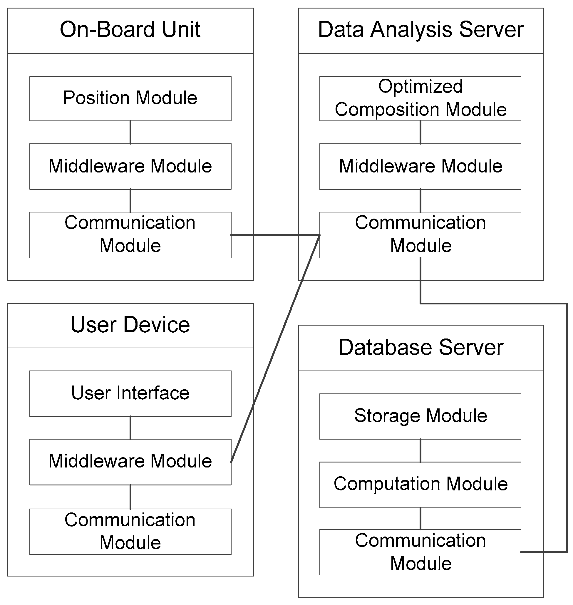
The proposed fuel consumption estimation system includes OBUs, user devices, a data analysis server, and a database server (shown in Figure 1). The OBU can send the movement information which includes the timestamp, location (i.e., longitude and latitude), and vehicle speed to the data analysis server. Furthermore, a user can use his user device to input the fuel quantity after refuelling. The data analysis server can store these data in the database server and perform a fuel consumption estimation method to estimate fuel consumption in accordance with the pattern of driver behaviour.

2.1. On-Board Unit

The OBU includes a position module, a middleware module, and a communication module as follows.

• The position module can support a global positioning system (GPS) to receive and analyze satellite signals for estimating the location (i.e., longitude and latitude) and speed of the vehicle.
• The communication module can support the techniques of long term evolution (LTE), and the OBU can connect with the data analysis server through the communication module and cellular networks.
• The middleware module can support hypertext transfer protocol (HTTP) and representational state transfer (REST), and the OBU can periodically call application program interfaces (APIs) and send the movement information (e.g., OBU ID, car type, driver ID, timestamp, longitude, latitude, and vehicle speed) to the data analysis server.

In this study, an OBU stores an OBU ID, a car type, and a driver ID. There are C_N OBUs, T_N car types, and D_N drivers. The OBU can send the movement information to the data analysis server every 30 s. For instance, Driver 1 drove the car which was equipped with OBU 1 on 1 January 2015, and the type of this car was Type 1. The position module of OBU 1 was used to estimate the location (i.e., 120.5423383° E and 24.09490167° N) and speed (i.e., 44 km/h) at 06:00:00, and the middleware module was used to call REST APIs of the data analysis server for the transmission of the movement information (shown in

Table 1. Movement information.

OBU ID	Car Type	Driver ID	Time	Longitude	Latitude	Speed (km/h)
OBU 1	Type 1	Driver 1	1 January 2015 06:00:00	120.5423383	24.09490167	44
OBU 1	Type 1	Driver 1	1 January 2015 06:00:30	120.5361317	24.09120167	39
OBU 1	Type 1	Driver 1	1 January 2015 06:01:00	120.5360417	24.09114667	2
OBU 1	Type 1	Driver 1	1 January 2015 06:01:30	120.5360383	24.09115	0
OBU 1	Type 1	Driver 1	1 January 2015 06:02:00	120.536035	24.09113833	0
OBU 1	Type 1	Driver 1	1 January 2015 06:02:30	120.5356167	24.09070333	7
OBU 1	Type 1	Driver 1	1 January 2015 06:03:00	120.53052	24.09449167	48
OBU 1	Type 1	Driver 1	1 January 2015 06:03:30	120.52868	24.09591167	30
…
OBU CN	Type TN	Driver DN	31 December 2015 22:00:00	121.0601083	24.75685833	102

OBU: On-board unit.

).

2.2. User Device

The user device includes a user interface, a middleware module, and a communication module as follows.

• The user interface can be used to input the OBU ID, timestamp, and fuel quantity after refuelling.
• The communication module can support the techniques of LTE, and the connection between a user device and the data analysis server can be built through the communication module.
• The middleware module can support the techniques of HTTP and REST, and the user device can send the information such as OBD ID, timestamp, and fuel quantity to the data analysis server through the middleware module.

In this study, a user can input the information of fuel quantity (e.g., OBU ID, timestamp, and fuel quantity) through the user interface of the user device after refuelling, and the fuel quantity information can be sent to the data analysis server through the middleware module. For instance, the car which was equipped with OBU 1 was refueled with 43.04 L of gas at 18:51:00 on 5 January 2015. Then a user inputted the OBU ID (i.e., OBU 1), timestamp (i.e., 5 January 2015 18:51:00), and fuel quantity (i.e., 43.03 L) through the user interface of the user device, and the middleware module was used to send the inputted data (i.e., the fuel quantity information) to the data analysis server (shown in

Table 2. Fuel quantity information.

OBU ID	Time	Fuel Quantity (L)
OBU 1	5 January 2015 18:51:00	43.04
OBU 1	6 January 2015 21:11:00	47.11
OBU 1	8 January 2015 17:49:00	31.81
OBU 1	10 January 2015 20:35:00	21.50
OBU 1	12 January 2015 19:59:00	41.16
OBU 1	14 January 2015 11:36:00	34.43
OBU 1	15 January 2015 19:18:00	27.75
OBU 1	16 January 2015 19:15:00	38.26
…
OBU CN	31 December 2015 23:00:00	51.79

).

2.3. Data Analysis Server

The data analysis server includes a middleware module, communication module, and an optimized composition module as follows.

• The middleware module can obtain several REST APIs to receive the movement information (e.g., OBU ID, car type, driver ID, timestamp, longitude, latitude, and vehicle speed) and the fuel quantity information (e.g., OBU ID, timestamp, and fuel quantity) from the OBUs and user devices through HTTP. These data can be stored in a database server.
• The communication module can support Ethernet and build the connections among the data analysis server and other devices (e.g., OBUs, user devices, and a database server).
• The optimized composition module can use the proposed fuel consumption estimation method to collect and analyse the movement information and fuel quantity information for generating the estimated results of fuel consumption.

In this study, the data analysis server can request Google Maps [20] or Chunghwa Telecom GeoWeb [21] to find the corresponding road type of the location through the middleware module. For instance, the road type of the location which is positioned at 120.5423383° E and 24.09490167° N is an urban road. The data analysis server can add the column of road type into the movement information (shown in

Table 3. The modified movement information.

OBU ID	Car Type	Driver ID	Time	Longitude	Latitude	Road Type	Speed (km/h)
OBU 1	Type 1	Driver 1	1 January 2015 06:00:00	120.5423383	24.09490167	Urban	44
OBU 1	Type 1	Driver 1	1 January 2015 06:00:30	120.5361317	24.09120167	Urban	39
OBU 1	Type 1	Driver 1	1 January 2015 06:01:00	120.5360417	24.09114667	Urban	2
OBU 1	Type 1	Driver 1	1 January 2015 06:01:30	120.5360383	24.09115	Urban	0
OBU 1	Type 1	Driver 1	1 January 2015 06:02:00	120.536035	24.09113833	Urban	0
OBU 1	Type 1	Driver 1	1 January 2015 06:02:30	120.5356167	24.09070333	Urban	7
OBU 1	Type 1	Driver 1	1 January 2015 06:03:00	120.53052	24.09449167	Urban	48
OBU 1	Type 1	Driver 1	1 January 2015 06:03:30	120.52868	24.09591167	Urban	30
…
OBU CN	Type TN	Driver DN	31 December 2015 22:00:00	121.0601083	24.75685833	Highway	102

), and the modified movement information can be stored in a database server.

2.4. Database Server

The database server includes a storage module, a computation module, and a communication module as follows.

• The communication module can support Ethernet, and the connection between the database server and the data analysis server can be built by this module.
• The computation module can receive the requests from the data analysis server through the communication module and access the storage module in accordance with the requests.
• The storage module can perform the operations of creation, update, deletion, and query.

3. Fuel Consumption Estimation Method

This study proposes a fuel consumption estimation method which includes a movement information collection method, a fuel information collection method, and an optimized composition method. The details of each method are illustrated in the following subsections.

3.1. Movement Information Collection Method

The process of the movement information collection method includes: (1) receiving the movement information from the OBUs; (2) analyzing and storing the movement information; and (3) calculating the amount of each vehicle speed interval (i.e., driver behaviour in this study) for each OBU and each driver during a time interval.

In this study, the movement information collection method can be performed by the optimized composition module of the data analysis server to retrieve the modified movement information (shown in Table 3). The vehicle speed (v) of each movement record can be converted into a vehicle speed interval, and the amount of each vehicle speed interval for each OBU and each driver during a time interval can be calculated. This study chooses 10 km/h as a vehicle speed interval and one year as a time interval for the estimation of driver behaviour. For instance, Driver 1 drove a car which was equipped with OBU 1 during 2015; $c_{1,1,1}^{C,D}$ records which include idle speed (i.e., the value of v is zero) are reported by OBU 1 during 2015; $c_{1,1,2}^{C,D}$ records which include the speed between 0 km/h and 10 km/h are reported by OBU 1 during 2015; consequently, $c_{1,1,14}^{C,D}$ records which include the speed higher than 120 km/h are reported by OBU 1 during 2015. Furthermore, Driver D_N drove a car which was equipped OBU C_N during 2015; $c_{C_N,D_N,1}^{C,D}$ records which include idle speed are reported by OBU C_N during 2015; $c_{C_N,D_N,2}^{C,D}$ records which include the speed between 0 km/h and 10 km/h are reported by OBU C_N during 2015; consequently, $c_{C_{N,D_N},14}^{C,D}$ records which include the speed higher than 120 km/h are reported by OBU C_N during 2015 (shown in

Table 4. The movement information of each OBU and each driver during 2015 (The unit of v is km/h).

	Movement	$\mathit{v}=0$	$0<\mathit{v}\le 10$	$10<\mathit{v}\le 20$	…	$110<\mathit{v}\le 120$	$120<\mathit{v}$
OBU ID and Driver ID
Driver 1 drove OBU 1		$c_{1,1,1}^{C,D}$	$c_{1,1,2}^{C,D}$	$c_{1,1,3}^{C,D}$	…	$c_{1,1,13}^{C,D}$	$c_{1,1,14}^{C,D}$
Driver 2 drove OBU 1		$c_{1,2,1}^{C,D}$	$c_{1,2,2}^{C,D}$	$c_{1,2,3}^{C,D}$	…	$c_{1,2,13}^{C,D}$	$c_{1,2,14}^{C,D}$
…		…	…	…	…	…	…
Driver 1 drove OBU 2		$c_{2,1,1}^{C,D}$	$c_{2,1,2}^{C,D}$	$c_{2,1,3}^{C,D}$	…	$c_{2,1,13}^{C,D}$	$c_{2,1,14}^{C,D}$
…		…	…	…	…	…	…
Driver DN drove OBU CN		$c_{C_N,D_N,1}^{C,D}$	$c_{C_N,D_N,2}^{C,D}$	$c_{C_N,D_N,3}^{C,D}$	…	$c_{C_N,D_N,13}^{C,D}$	$c_{C_{N,D_N},14}^{C,D}$

).

For precise estimation of driver behaviour, this study also chooses one month as a time interval. For instance, Driver 1 drove a car which was equipped with OBU 1; ${c_1}_{1,1,1}^{C,D}$ records which include idle speed are reported by OBU 1 during January 2015; consequently, ${c_M}_{1,1,1}^{C,D}$ records which include idle speed are reported by OBU 1 during the M-th month of 2015. Therefore, the summary of each monthly record of 2015 is equal to the yearly record (i.e., ${\displaystyle \sum _{M=1}^{12}{c_M}_{1,1,1}^{C,D}}=c_{1,1,1}^{C,D}$).

3.2. Fuel Information Collection Method

The process of the fuel information collection method includes: (1) receiving the fuel quantity information from the user devices; (2) analyzing and storing the fuel quantity information; and (3) calculating the amount of fuel quantities for each OBU and each driver during a time interval.

In this study, the fuel information collection method can retrieve the fuel quantity information (shown in Table 2) and analyse the amount of fuel quantities for each OBU and each driver during a time interval. This study chooses one month or one year as a time interval. For instance, Driver 1 drove a car which was equipped with OBU 1 during 2015; the summary of fuel quantities of OBU 1 during January 2015 is ${Q_1}_{1,1}^{C,D}$ L; the summary of fuel quantities of OBU 1 during the M-th of 2015 is ${Q_M}_{1,1}^{C,D}$ L; consequently, the summary of fuel quantities of OBU 1 during 2015 is $Q_{1,1}^{C,D}$ L (i.e., ${\displaystyle \sum _{M=1}^{12}{Q_M}_{1,1}^{C,D}}=Q_{1,1}^{C,D}$). Furthermore, Driver D_N drove a car which was equipped with OBU C_N during 2015; the summary of fuel quantities of OBU C_N during January 2015 is ${Q_1}_{C_N,D_N}^{C,D}$ L; the summary of fuel quantities of OBU C_N during the M-th of 2015 is ${Q_M}_{C_N,D_N}^{C,D}$ L; consequently, the summary of fuel quantities of OBU C_N during 2015 is $Q_{C_N,D_N}^{C,D}$ L (i.e., ${\displaystyle \sum _{M=1}^{12}{Q_M}_{C_N,D_N}^{C,D}}=Q_{C_N,D_N}^{C,D}$).

3.3. Optimized Composition Method

In this subsection, the design of the optimized composition method is presented in Section 3.3.1, and a case study of this method is given in Section 3.3.2.

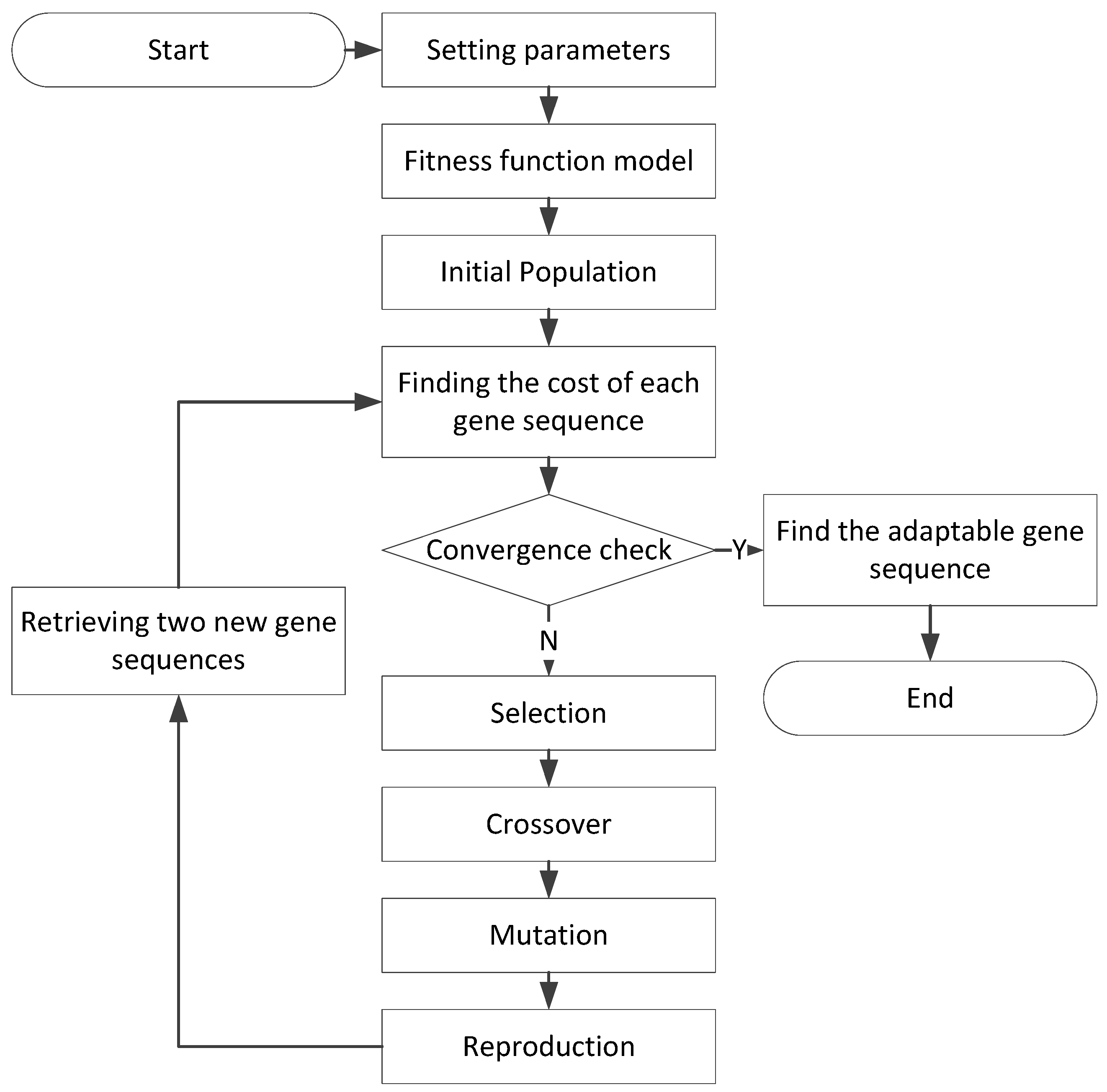
3.3.1. The Process of the Method

The process of the optimized composition method includes: (1) receiving the patterns of driver behaviours from the movement information collection method; (2) receiving the patterns of fuel consumption from the fuel information collection method; and (3) performing a GA (shown in Figure 2) to analyse the set of fuel consumption in accordance with the pattern of driver behaviour. The steps of the optimized composition method are illustrated as follows.

• The values of the parameters including the amount of initial maternal DNA (deoxyribonucleic acid) sequences ($coun{t}_g$), the number of evolution times ($coun{t}_c$), the maximum number of iterations ($coun{t}_i$), crossover rate (α), and mutation rate (β) are initially given in this step.
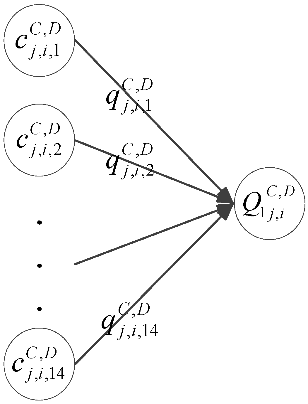
• The model of fitness function is designed for finding the cost of each DNA sequence which includes several chromosomes.
• The process of the initial population can generate $coun{t}_g$ maternal DNA sequences.
• Each DNA sequence can be adopted into the model of fitness function for the cost calculation.
• The process of the convergence check can be performed to check the values of the number of evolution times ($coun{t}_c$) and the maximum number of iterations ($coun{t}_i$). If the number of evolution times ($coun{t}_c$) is equal to the maximum number of iterations ($coun{t}_i$), the adaptable DNA sequence with the lowest cost is outputted as the estimated results of the fuel consumption based on the driver behaviour; otherwise the number of evolution times ($coun{t}_c$) is increased by one.
• The process of gene selection can select two of the maternal DNA sequences for crossover and mutation.
• The process of gene crossover can generate a child’s DNA sequences in the first generation in accordance with the crossover rate (α) and the maternal DNA sequences in the first generation.
• The process of gene mutation can generate a child’s DNA sequences in the second generation in accordance with the mutation rate (β) and the maternal DNA sequences in the second generation.
• The process of gene reproduction can support two new generated child’s DNA sequences being substituted for two original maternal DNA sequences which have the highest cost.
• The costs of the two reproduced DNA sequences can be measured by using the model of fitness function, and the GA is performed repeatedly.

3.3.2. A Case Study

The parameters of GA in this study are adopted as follows: the amount of initial maternal DNA sequences ($coun{t}_g$) is 14; the initial number of evolution times ($coun{t}_c$) is 0; the maximum number of iterations ($coun{t}_i$) is 1000; the crossover rate (α) is 100%; the mutation rate (β) is 7%. A DNA sequence $q_{j,i}^{C,D}=\left\{q_{j,i,1}^{C,D},q_{j,i,2}^{C,D},...,q_{j,i,14}^{C,D}\right\}$ includes 14 chromosomes (i.e., $\left|q_{j,i}^{C,D}\right|=14$) for the j-th OBU driven by the i-th driver. Each chromosome is encoded as a float. For instance, the parameter $q_{j,i,1}^{C,D}$ can be used to estimate the quantity of fuel consumption at idle speed during each 30 s period for the j-th OBU driven by the i-th driver. Furthermore, the model of fitness function $s=\left|\left[{\displaystyle \sum _{k=1}^{14}\left(c_{j,i,k}^{C,D}\times q_{j,i,k}^{C,D}\right)}\right]-Q_{j,i}^{C,D}\right|$ (shown in Figure 3) is adopted to estimate the cost of each DNA sequence. The unit of cost is a liter in this model. The best DNA sequence has the lowest cost (i.e., $s=\left|\left[{\displaystyle \sum _{k=1}^{14}\left(c_{j,i,k}^{C,D}\times q_{j,i,k}^{C,D}\right)}\right]-Q_{j,i}^{C,D}\right|=0$) in this study.

For the initial population, 14 maternal DNA sequences are randomly generated, and each DNA sequence includes 14 chromosomes. For instance, the first maternal DNA sequence is ${q_1}_{j,i}^{C,D}=\left\{{q_1}_{j,i,1}^{C,D},{q_1}_{j,i,2}^{C,D},...,{q_1}_{j,i,14}^{C,D}\right\}$ for the j-th OBU driven by the i-th driver; the second maternal DNA sequence is ${q_2}_{j,i}^{C,D}=\left\{{q_2}_{j,i,1}^{C,D},{q_2}_{j,i,2}^{C,D},...,{q_2}_{j,i,14}^{C,D}\right\}$ for the j-th OBU driven by the i-th driver; consequently, the fourteenth maternal DNA sequence is ${q_{14}}_{j,i}^{C,D}=\left\{{q_{14}}_{j,i,1}^{C,D},{q_{14}}_{j,i,2}^{C,D},...,{q_{14}}_{j,i,14}^{C,D}\right\}$ for the j-th OBU driven by the i-th driver (shown in

Table 5. Maternal DNA sequences.

	Chromosome	Chromosome 1	Chromosome 2	…	Chromosome 14
DNA Sequences
DNA Sequence 1 (${q_1}_{j,i}^{C,D}$)		${q_1}_{j,i,1}^{C,D}$	${q_1}_{j,i,2}^{C,D}$	…	${q_1}_{j,i,14}^{C,D}$
DNA Sequence 2 (${q_2}_{j,i}^{C,D}$)		${q_2}_{j,i,1}^{C,D}$	${q_2}_{j,i,2}^{C,D}$	…	${q_2}_{j,i,14}^{C,D}$
…
DNA Sequence 14 (${q_{14}}_{j,i}^{C,D}$)		${q_{14}}_{j,i,1}^{C,D}$	${q_{14}}_{j,i,2}^{C,D}$	…	${q_{14}}_{j,i,14}^{C,D}$

).

This study gives a case study of OBU 1 driven by Driver 1 to explain the process of the optimized composition method. The set of movement information of OBU 1 driven by Driver 1 during 2015 is recorded as $C_{1,1}^{C,D}=\left\{c_{1,1,1}^{C,D},c_{1,1,2}^{C,D},...,c_{1,1,14}^{C,D}\right\}=\left\{103100,66752,...,4\right\}$, and the fuel quantity of OBU 1 driven by Driver 1 during 2015 is recorded as 10921.364 L (i.e., $Q_{1,1}^{C,D}=10921.364$). Furthermore, the 14 maternal DNA sequences are randomly generated as shown in

Table 6. The maternal DNA sequence for OBU 1 driven by Driver 1.

	Chromosome	Chromosome 1	Chromosome 2	…	Chromosome 14
DNA Sequences
DNA Sequence 1 (${q_1}_{j,i}^{C,D}$)		0.013249146	0.018487159	…	0.551971137
DNA Sequence 2 (${q_2}_{j,i}^{C,D}$)		0.016574516	0.02331678	…	0.553625064
…
DNA Sequence 14 (${q_{14}}_{j,i}^{C,D}$)		0.01539256	0.021892833	…	0.555117159

. For example, the first maternal DNA sequence is $q_{11,1}^{ C,D}=\left\{0.013249146,0.018487159,...,0.551971137\right\}$; the second maternal DNA sequence is $q_{21,1}^{ C,D}=\left\{0.016574516,0.02331678,...,0.553625064\right\}$; consequently, the fourteenth maternal DNA sequence is $q_{141,1}^{\hspace{1em}C,D}=\left\{0.01539256,0.021892833,...,0.555117159\right\}$.

For finding the cost of each DNA sequence, the set of chromosomes in a maternal DNA sequence is adopted into the fitness function. In this study, the cost of the h-th maternal DNA sequence is defined as $s_h=\left|\left[{\displaystyle \sum _{k=1}^{14}\left(c_{j,i,k}^{C,D}\times {q_h}_{j,i,k}^{C,D}\right)}\right]-Q_{j,i}^{C,D}\right|$ for the j-th OBU driven by the i-th driver. For instance, the cost of the first maternal DNA sequence is calculated by Equation (1) for OBU 1 driven by Driver 1; the cost of the second maternal DNA sequence is calculated by Equation (2) for OBU 1 driven by Driver 1; consequently, the cost of the fourteenth maternal DNA sequence is calculated by Equation (3) for OBU 1 driven by Driver 1.

$$\begin{array}{ll}{s}_1& =\left|\left(103100\times 0.013249146+66752\times 0.018487159+...+4\times 0.551971137\right)-10921.364\right|\\ & =260.2534752\end{array}$$

(1)

$$\begin{array}{ll}{s}_2& =\left|\left(103100\times 0.016574516+66752\times 0.02331678+...+4\times 0.553625064\right)-10921.364\right|\\ & =1062.546744\end{array}$$

(2)

$$\begin{array}{ll}{s}_{14}& =\left|\left(103100\times 0.01539256+66752\times 0.021892833+...+4\times 0.555117159\right)-10921.364\right|\\ & =1009.53678\end{array}$$

(3)

For the convergence check, the adaptable DNA sequence with the lowest cost is output as the estimated results of the fuel consumption based on driver behaviour if the number of evolution times ($coun{t}_c$) is equal to the maximum number of iterations ($coun{t}_i$); otherwise the number of evolution times ($coun{t}_c$) is increased by one.

For gene selection, this study uses the roulette wheel selection method to select two of the maternal DNA sequences. For instance, DNA Sequence 1 ($q_{11,1}^{ C,D}=\left\{0.013249146,0.018487159,...,0.551971137\right\}$) and DNA Sequence 2 ($q_{21,1}^{ C,D}=\left\{0.016574516,0.02331678,...,0.553625064\right\}$) (shown in

Table 7. The maternal DNA sequences in the first generation.

	Chromosome	Chromosome 1	Chromosome 2	…	Chromosome 14
DNA Sequences
DNA Sequence 1 ($q_{11,1}^{ C,D}$)		0.013249146	0.018487159	…	0.551971137
DNA Sequence 2 ($q_{21,1}^{ C,D}$)		0.016574516	0.02331678	…	0.553625064

) are selected as the maternal DNA sequences in the first generation for OBU 1 driven by Driver 1.

For gene crossover, the 1-point crossover method is performed in accordance with the crossover rate (α). For instance, the value of the crossover point is randomly determined as 2. Then the two child’s DNA sequences (shown in

Table 8. The child’s DNA sequences in the first generation.

	Chromosome	Chromosome 1	Chromosome 2	…	Chromosome 14
DNA Sequences
DNA Sequence 1 ${\left({q_1}_{1,1}^{C,D}\right)}^{\prime }$		0.013249146	0.02331678	…	0.553625064
DNA Sequence 2 ${\left({q_2}_{1,1}^{C,D}\right)}^{\prime }$		0.016574516	0.018487159	…	0.551971137

) are generated as Equations (4) and (5) according to the two maternal DNA sequences (shown in Table 7). The line in Equations (4) and (5) is the crossover point.

$$\mathrm{DNA} \mathrm{Sequence} 1 \begin{array}{cc}\hfill {\left(q_{11,1}^{ C,D}\right)}^{\prime }=& \left\{{\left(q_{11,1,1}^{ C,D}\right)}^{\prime },{\left(q_{11,1,2}^{ C,D}\right)}^{\prime },...,{\left(q_{11,1,14}^{ C,D}\right)}^{\prime }\right\}\hfill \\ & =\left\{0.013249146,|0.02331678,...,0.553625064\right\}\hfill \end{array}$$

(4)

$$\mathrm{DNA} \mathrm{Sequence} 2 \begin{array}{cc}\hfill {\left(q_{21,1}^{ C,D}\right)}^{\prime }=& \left\{{\left(q_{21,1,1}^{ C,D}\right)}^{\prime },{\left(q_{21,1,2}^{ C,D}\right)}^{\prime },...,{\left(q_{21,1,14}^{ C,D}\right)}^{\prime }\right\}\hfill \\ & =\left\{0.016574516,|0.018487159,...,0.551971137\right\}\hfill \end{array}$$

(5)

For gene mutation, the set of binary vectors ($\eta =\left\{{\eta }_1,{\eta }_2,...,{\eta }_{14}\right\}$) is randomly generated in accordance with the mutation rate (β). If the value of ${\eta }_n$ is equal to one, the value of the n-th chromosome will be changed after the process of gene mutation. For instance, the child’s DNA sequences in the first generation (shown in Table 8) are selected as the maternal DNA sequences in the second generation (shown in

Table 9. The maternal DNA sequences in the second generation.

	Chromosome	Chromosome 1	Chromosome 2	…	Chromosome 14
DNA Sequences
DNA Sequence 1 $\left({q_1}_{1,1}^{C,D}\right)$		0.013249146	0.02331678	…	0.553625064
DNA Sequence 2 $\left({q_2}_{1,1}^{C,D}\right)$		0.016574516	0.018487159	…	0.551971137

). Furthermore, the set of binary vectors is randomly generated as $\eta =\left\{1,0,0,0,0,0,0,0,0,0,0,0,0,0\right\}$. Then the two child’s DNA sequences (shown in

Table 10. The child’s DNA sequences in the second generation.

	Chromosome	Chromosome 1	Chromosome 2	…	Chromosome 14
DNA Sequences
DNA Sequence 1 ${\left({q_1}_{1,1}^{C,D}\right)}^{\prime }$		0.011241019	0.02331678	…	0.553625064
DNA Sequence 2 ${\left({q_2}_{1,1}^{C,D}\right)}^{\prime }$		0.012500034	0.018487159	…	0.551971137

) are determined according to the two maternal DNA sequences (shown in Table 9).

For gene reproduction, the two new generated child’s DNA sequences are substituted for two of the original maternal DNA sequences which have the highest cost. For instance, the costs of DNA Sequence 2 (${q_2}_{j,i}^{C,D}$) and DNA Sequence 14 (${q_{14}}_{j,i}^{C,D}$) are higher than the costs of the other maternal DNA sequences in Table 6 for OBU 1 driven by Driver 1. Therefore, the two new generated child’s DNA sequences in Table 10 are substituted for DNA Sequence 2 (${q_2}_{j,i}^{C,D}$) and DNA Sequence 14 (${q_{14}}_{j,i}^{C,D}$) (shown in

Table 11. The maternal DNA sequences after the first iteration.

	Chromosome	Chromosome 1	Chromosome 2	…	Chromosome 14
DNA Sequences
DNA Sequence 1 ($q_{11,1}^{ C,D}$)		0.013249146	0.018487159	…	0.551971137
DNA Sequence 2 (${q_2}_{1,1}^{C,D}={\left({q_1}_{1,1}^{C,D}\right)}^{\prime }$)		0.011241019	0.02331678	…	0.553625064
…
DNA Sequence 14 (${q_{14}}_{1,1}^{C,D}={\left({q_2}_{1,1}^{C,D}\right)}^{\prime }$)		0.012500034	0.018487159	…	0.551971137

). Furthermore, the costs of these two reproduced DNA sequences are determined by Equations (6) and (7), respectively.

$$\begin{array}{ll}{s}_2& =\left|\left(103100\times 0.011241019+66752\times 0.02331678+...+4\times 0.553625064\right)-10921.364\right|\\ & =512.663178\end{array}$$

(6)

$$\begin{array}{ll}{s}_{14}& =\left|\left(103100\times 0.01539256+66752\times 0.021892833+...+4\times 0.555117159\right)-10921.364\right|\\ & =183.020039\end{array}$$

(7)

After gene reproduction, the convergence check is performed repeatedly. The adaptable DNA sequence with the lowest cost is output as the estimated results of the fuel consumption based on the driver behaviour when the number of evolution times ($coun{t}_c$) is equal to the maximum number of iterations ($coun{t}_i$). In the case of OBU 1 driven by Driver 1 in this study, the adaptable DNA sequence with the lowest cost, DNA Sequence 14 (${q_{14}}_{j,i}^{C,D}$), is output as the estimated results of the fuel consumption based on the driver behaviour (shown in Equation (8)). Therefore, the parameter $q_{1,1,1}^{C,D}$ (i.e., 0.0125003 L) is used to estimate the quantity of fuel consumption at idle speed during each 30 s period; consequently, the quantity of fuel consumption at higher speed (>120 km/h) during each 30 s period is estimated as $q_{1,1,14}^{C,D}$ (i.e., 0.551971137 L).

$$\begin{array}{ll}{q}_{1,1}^{C,D}& ={q_{14}}_{1,1}^{C,D}\\ & =\left\{q_{1,1,1}^{C,D},q_{1,1,2}^{C,D},...,q_{1,1,14}^{C,D}\right\}\\ & =\left\{\begin{array}{l}0.012500034,0.018487159,0.035458125,0.064768478,0.088150596,\\ 0.036826864,0.070565879,0.095323361,0.154325441,0.149250046,\\ 0.063605949,0.045212032,0.132129733,0.551971137\end{array}\right\}\end{array}$$

(8)

4. Practical Experimental Results and Discussions

This section describes the practical experimental environments and data, and some experimental designs are given to evaluate the proposed method in the following subsections.

4.1. Experimental Environments

The practical experimental data including the movement information and fuel quantity of fifteen trucks during November and December 2016 were collected from an eFMS (e-Fleet Management Service) system which was built by Chunghwa Telecom [22] for the evaluation of the proposed method. This study used the Package ‘GA’ [23] to implement the GA algorithm for fuel consumption estimation. The movement information and fuel quantity information during November 2016 were used as training data, and the movement information and fuel quantity information during December 2016 were used as testing data to evaluate the performance of the proposed fuel consumption estimation system and method. In the training data, 420,673 movement records were retrieved, and 105,569 km were driven by the trucks; in the testing data, 414,798 movement records were retrieved, and 107,651 km were driven by the trucks (shown in

Table 12. The movement information in practical experimental environments.

OBU ID	November 2016 (i.e., Training Data)		December 2016 (i.e., Testing Data)
	The Number of Movement Records	Driving Mileage (km)	The Number of Movement Records	Driving Mileage (km)
1	29,115	10,636	33,546	13,548
2	39,957	11,598	39,573	12,500
3	29,289	7897	28,097	6825
4	18,980	2844	15,313	2211
5	23,514	5928	22,015	5418
6	26,422	4880	28,820	5964
7	32,345	9404	34,440	10,258
8	30,859	6707	29,066	6195
9	36,165	10,316	34,445	10,229
10	30,046	6419	28,199	6367
11	26,074	5884	26,301	5917
12	19,258	5340	19,191	5337
13	26,106	5720	26,353	6067
14	24,620	5475	24,252	5066
15	27,923	6520	25,187	5749
Summary	420,673	105,569	414,798	107,651

).

Table 13. The fuel quantity information in practical experimental environments.

OBU ID	November 2016 (i.e., Training Data)		December 2016 (i.e., Testing Data)
	The Number of Refuelling Times	Fuel Quantity (L)	The Number of Refuelling Times	Fuel Quantity (L)
1	20	3619.020	25	4582.252
2	21	3820.000	24	4180.871
3	16	2704.016	15	2425.483
4	15	581.154	11	479.641
5	23	1031.828	25	975.490
6	26	838.163	30	896.126
7	16	3222.007	18	3578.000
8	14	2440.178	14	2331.264
9	23	3662.796	22	3691.831
10	17	2334.016	18	2350.214
11	11	2100.003	12	2241.000
12	30	897.420	25	874.300
13	15	2166.003	16	2296.017
14	20	1690.028	20	1782.006
15	13	581.154	11	479.641
Summary	280	31,687.786	286	33,164.136

shows that the fuel quantity was about 31,687.786 L from 280 refuelling times in the training data, and the fuel quantity was about 33,164.136 L from 286 refuelling times in the testing data.

4.2. Experimental Designs

Three cases were designed to evaluate the performances of the fuel consumption estimation with or without road types. Furthermore, this study compared the performances of the proposed method and the fuel economy guide [24]. Each case is illustrated as follows.

• Case 1: The fuel consumption estimation method considered the different road types (e.g., urban road and highway). In this case, each DNA sequence included 28 chromosomes.
• Case 2: The fuel consumption estimation method did not consider the different road types. In this case, each DNA sequence included 14 chromosomes.
• Case 3: The significant differences between the results of Case 1 and Case 2 were evaluated.

In this study, the mean absolute percentage error (MAPE) was used to measure the accuracy of the fuel consumption estimation method by Equation (9). Furthermore, the t-test and F-test were adopted to evaluate the significant differences between the results of Case 1 and Case 2.

$$accuracy=100\%-MAPE=100\%-\frac{\left|real\_value-estimated\_value\right|}{real\_value}$$

(9)

4.3. Experimental Results and Discussions

This subsection used the records during November 2016 (i.e., training data) with the proposed method to retrieve the adaptable DNA sequence as the estimated fuel consumption based on the driver behaviour. Then the records during December 2016 (i.e., testing data) were used to test the performance of the proposed method. In Case 1 (i.e., 28 chromosomes), the testing results indicated that the accuracies of the proposed method and fuel economy guide were 95.54% and 24.06% (shown in

Table 14. The accuracy of fuel consumption estimation with road types (i.e., Case 1).

OBU ID	The Proposed Method		Fuel Economy Guide [24]
	Accuracy of Training Data	Accuracy of Testing Data	Accuracy of Training Data	Accuracy of Testing Data
1	99.73%	91.55%	16.89%	16.99%
2	99.70%	92.66%	17.45%	17.18%
3	99.28%	93.60%	16.78%	16.17%
4	99.49%	94.90%	28.12%	26.49%
5	99.95%	97.12%	33.02%	31.92%
6	98.76%	95.48%	33.46%	38.25%
7	99.34%	97.29%	16.77%	16.48%
8	99.80%	99.37%	15.80%	15.27%
9	99.62%	97.89%	16.19%	15.92%
10	99.00%	95.30%	15.81%	15.57%
11	99.68%	96.09%	16.10%	15.17%
12	99.47%	97.22%	34.20%	35.08%
13	99.65%	95.41%	15.18%	15.19%
14	94.36%	96.56%	18.62%	16.34%
15	99.39%	92.71%	64.48%	68.89%
Mean	99.15%	95.54%	23.92%	24.06%

), respectively. Furthermore,

Table 15. The accuracy of fuel consumption estimation without road types (i.e., Case 2).

OBU ID	The proposed Method		Fuel Economy Guide [24]
	Accuracy of Training Data	Accuracy of Testing Data	Accuracy of Training Data	Accuracy of Testing Data
1	99.54%	92.19%	16.89%	16.99%
2	98.99%	91.59%	17.45%	17.18%
3	98.86%	96.81%	16.78%	16.17%
4	97.26%	97.70%	28.12%	26.49%
5	99.79%	98.71%	33.02%	31.92%
6	98.24%	95.61%	33.46%	38.25%
7	99.77%	95.74%	16.77%	16.48%
8	99.71%	98.44%	15.80%	15.27%
9	98.90%	96.59%	16.19%	15.92%
10	99.02%	97.81%	15.81%	15.57%
11	99.04%	93.26%	16.10%	15.17%
12	99.88%	99.05%	34.20%	35.08%
13	96.85%	89.22%	15.18%	15.19%
14	97.23%	99.28%	18.62%	16.34%
15	98.77%	96.12%	64.48%	68.89%
Mean	98.79%	95.87%	23.92%	24.06%

shows that the accuracy of the proposed method was 95.87% in Case 2 (i.e., 14 chromosomes). The Bureau of Energy did not consider driver behaviour, traffic condition, and weather when it performed its experiments, so larger errors of fuel consumption estimation were generated in accordance with the fuel economy guide [24]. Therefore, the proposed method can provide precise fuel consumption estimation in practical environments for the logistics industries.

The practical data were collected from 15 trucks to evaluate the accuracy of the proposed method in Cases 1 and 2. In Case 3, a two-tailed t-test was performed to determine the differences between the mean accuracy of the proposed method in Case 1 and Case 2. The p-value of this two-tailed t-test was measured as 0.6396 which is higher than the alpha level of 0.05, so the H0 (i.e., null hypothesis) was accepted under 14 degrees of freedom (i.e., 14 = 15 − 1). Furthermore, this study performed a two-tailed F-test to determine the differences between the variance of the accuracy of the proposed method in Case 1 and Case 2. The p-value of this two-tailed F-test was measured as 0.1160 which is higher than the alpha level of 0.05, so the H0 (i.e., null hypothesis) was accepted under 14 degrees of freedom (i.e., 14 = 15 − 1). There were no significant differences between the results of Case 1 and Case 2. Therefore, the fuel consumption estimation without road types can be adopted for reducing the computation costs in the future.

5. Conclusions and Future Work

As monitoring and reducing fuel costs is the greatest challenge for the logistics industries and bus carriers, a fuel consumption estimation system and method based on a GA is proposed to collect the movement information and fuel quantity information for analyzing the relation of fuel consumption and driver behaviour. This study models the pattern of driver behaviour as a gene sequence, and the GA including crossover and mutation processes is used to retrieve an adaptable gene sequence. The adaptable gene sequence can be applied as the set of fuel consumption in accordance with the pattern of driver behaviour. In practical experimental environments, 835,471 movement records from 15 trucks were collected for the evaluation of the proposed method. The practical results indicated that the accuracy of the proposed fuel consumption estimation method was 95.87%, which was higher than the fuel economy guide from the Bureau of Energy in Taiwan.

In the future, the evaluation model of the driver performance can be designed based on the proposed fuel consumption estimation method. Furthermore, some suggestions and guidelines can be made based on the driver behaviours for the driver’s reference.

References

1. Iodice, P.; Senatore, A. Road transport emission inventory in a regional area by using experimental two-wheelers emission factors. In Proceedings of the World Congress on Engineering, London, UK, 3–5 July 2013. [Google Scholar]
2. Chan, S.Y. The Basic Information of Truck Freight Transportation. Taiwan Institute of Economic Research, 2016. Available online: https://goo.gl/7zZ9ZY (accessed on 2 February 2017).
3. Chan, S.Y. The Basic Information of Bus Transportation. Taiwan Institute of Economic Research, 2016. Available online: https://goo.gl/hJnzXe (accessed on 2 February 2017).
4. Iodice, P.; Senatore, A. Exhaust emissions of new high-performance motorcycles in hot and cold conditions. Int. J. Environ. Sci. Technol. 2015, 12, 3133–3144. [Google Scholar] [CrossRef]
5. Iodice, P.; Senatore, A. Analysis of a Scooter Emission Behavior in Cold and Hot Conditions: Modelling and Experimental Investigations; SAE Technical Paper 2012-01-0881; Society of Automotive Engineers: Warrendale, PN, USA, 2012. [Google Scholar] [CrossRef]
6. Zhang, Z.; Yu, X.; Han, W. Investigation of real-time fuel consumption measuring system. Int. J. Hybrid Inf. Technol. 2015, 8, 235–242. [Google Scholar] [CrossRef]
7. Zhang, J.; Feng, Y.; Shi, F.; Wang, G.; Ma, B.; Li, R.; Jia, X. Vehicle routing in urban areas based on the oil consumption weight-Dijkstra algorithm. IET Intell. Transp. Syst. 2016, 10, 495–502. [Google Scholar] [CrossRef]
8. Zhang, S.; Wu, Y.; Liu, H.; Huang, R.; Un, P.; Zhou, Y.; Fu, L.; Hao, J. Real-world fuel consumption and CO2 (carbon dioxide) emissions by driving conditions for light-duty passenger vehicles in China. Energy 2014, 69, 247–257. [Google Scholar] [CrossRef]
9. Chang, C.W.; Kuo, Y.C.; Tsai, Y.Y.; Kuo, Y.L. Vehicle Fuel Consumption Detection System and Detection Method. Patent CN105,628,125, 1 June 2016. [Google Scholar]
10. Toledo, G.; Shiftan, Y. Can feedback from in-vehicle data recorders improve driver behavior and reduce fuel consumption. Transp. Res. Part A Policy Pract. 2016, 94, 194–204. [Google Scholar] [CrossRef]
11. Silva, J.A.; Moura, F.; Garcia, B.; Vargas, R. Influential vectors in fuel consumption by an urban bus operator: Bus route, driver behavior or vehicle type. Transp. Res. Part D Transp. Environ. 2015, 38, 94–104. [Google Scholar] [CrossRef]
12. Castignani, G.; Derrmann, T.; Frank, R.; Engel, T. Driver behavior profiling using smartphones: A low-cost platform for driver monitoring. IEEE Intell. Transp. Syst. Mag. 2015, 7, 91–102. [Google Scholar] [CrossRef]
13. Yao, H.H.; Kuo, Y.C.; Shang, T.J. Method for Calculating Fuel Consumption during Driving and Driving Fuel Consumption Calculation System. U.S. Patent 20,130,253,813, 26 September 2013. [Google Scholar]
14. Magaña, V.C.; Organero, M.M. GATSF: Genetic algorithm to save fuel. In Proceedings of the 2012 IEEE International Conference on Consumer Electronics-Berlin, Berlin, Germany, 3–5 September 2012. [Google Scholar]
15. Bao, Y.; Chen, W. A personalized route search method based on joint driving and vehicular behavior recognition. In Proceedings of the 2016 IEEE MTT-S International Wireless Symposium, Shanghai, China, 14–16 March 2016. [Google Scholar]
16. Rocha, T.V.; Jeanneret, B.; Trigui, R.; Leclercq, L. How simplifying urban driving cycles influence fuel consumption estimation? Procedia-Soc. Behav. Sci. 2012, 48, 1000–1009. [Google Scholar] [CrossRef]
17. Whitley, D. A genetic algorithm tutorial. Stat. Comput. 1994, 4, 65–85. [Google Scholar] [CrossRef]
18. Rajasekar, N.; Basil, J.; Balasubramanian, K.; Priya, K.; Sangeetha, K.; Babu, T.S. Comparative study of PEM fuel cell parameter extraction using genetic algorithm. Ain Shams Eng. J. 2015, 6, 1187–1194. [Google Scholar] [CrossRef]
19. Lee, W.C.; Tsang, K.F.; Chi, H.R.; Hung, F.H.; Wu, C.K.; Chui, K.T.; Lau, W.H.; Leung, Y.W. A high fuel consumption efficiency management scheme for PHEVs using an adaptive genetic algorithm. Sensors 2015, 15, 1245–1251. [Google Scholar] [CrossRef] [PubMed]
20. Google. Google Maps; Google Inc.: Mountain View, CA, USA, 2005; Available online: https://maps.google.com (accessed on 30 June 2017).
21. The Telecommunication Laboratories. Chunghwa GeoWeb Service; The Telecommunication Laboratories, Chunghwa Telecom Co., Ltd.: Taoyuan, Taiwan, 2007; Available online: http://demo.map.hinet.net/ (accessed on 30 June 2017).
22. The Telecommunication Laboratories. eFMS (e-Fleet Management Service); The Telecommunication Laboratories, Chunghwa Telecom Co., Ltd.: Taoyuan, Taiwan, 2014; Available online: http://efms.hinet.net/ (accessed on 9 March 2017).
23. Scrucca, L. Package ‘GA’, the Comprehensive R Archive Network. 2016. Available online: https://cran.r-project.org/web/packages/GA/ (accessed on 26 June 2017).
24. The Bureau of Energy. Fuel Economy Guide; The Bureau of Energy Ministry of Economic Affairs: Taipei, Taiwan, 2016. Available online: https://goo.gl/YpgQ9Q (accessed on 9 March 2017).
Figure 1. The architecture of the fuel consumption estimation system.
Symmetry 09 00105 g001
Figure 2. The process of the fuel consumption estimation method.
Symmetry 09 00105 g002
Figure 3. The model of the fitness function.
Symmetry 09 00105 g003