Path Embeddings with Prescribed Edge in the Balanced Hypercube Network

Abstract

The balanced hypercube network, which is a novel interconnection network for parallel computation and data processing, is a newly-invented variant of the hypercube. The particular feature of the balanced hypercube is that each processor has its own backup processor and they are connected to the same neighbors. A Hamiltonian bipartite graph with bipartition $V_0\cup V_1$ is Hamiltonian laceable if there exists a path between any two vertices $x\in V_0$ and $y\in V_1$. It is known that each edge is on a Hamiltonian cycle of the balanced hypercube. In this paper, we prove that, for an arbitrary edge e in the balanced hypercube, there exists a Hamiltonian path between any two vertices x and y in different partite sets passing through e with $e\ne xy$. This result improves some known results.

1. Introduction

Interconnection networks play an essential role in the performance of parallel and distributed systems. In the event of practice, large multi-processor systems can also be adopted as tools to address complex management and big data problems. It is well-known that an interconnection network is generally modeled by an undirected graph, in which processors are represented by vertices and communication links between them are represented by edges. The hypercube network is recognized as one of the most popular interconnection networks, and it has gained great attention and recognition from researchers both in graph theory and computer science. Nevertheless, the hypercube also has some shortcomings. For example, its diameter is large. Therefore, many variants of the hypercube have been put forward [1,2,3,4,5,6,7,8,9,10] to improve performance of the hypercube in some aspects. Among these variants, the balanced hypercube has the following special properties: each vertex of the balanced has a backup (matching) vertex and they have the same neighborhood. Therefore, the backup vertex can undertake tasks that originally run on a faulty vertex. It has been proved that the diameter of an odd-dimensional balanced hypercube $B{H}_n$ is $2n-1$ [10], which is smaller than that of the hypercube $Q_{2n}$.

With regard to the special properties discussed above, the balanced hypercube has been investigated by many researchers. Huang and Wu [11] studied the problem of resource placement of the balanced hypercube. Xu et al. [12] showed that the balanced hypercube is edge-pancyclic and Hamiltonian laceable. It is found that the balanced hypercube is bipanconnected for all $n\ge 1$ by Yang [13]. Huang et al. [14] discussed area efficient layout problems of the balanced hypercube. Yang [15] determined super (edge) connectivity of the balanced hypercube. Lü et al. studied (conditional) matching preclusion, hyper-Hamiltonian laceability, matching extendability and extra connectivity of the balanced hypercube in [16,17,18,19], respectively. Some symmetric properties of the balanced hypercube are presented in [20,21]. As stated above, the balanced hypercube possesses some desirable properties that the hypercube does not have, so it is interesting to explore other favorable properties that the balanced hypercube may have.

Since parallel applications such as image and signal processing are originally designed on array and ring architectures, it is important to have path and cycle embeddings in a network. Especially, Hamiltonian path and cycle embeddings and other properties of famous networks are extensively studied by many authors [12,13,22,23,24,25,26]. Xu et al. [12] proved that each edge of the balanced hypercube is on a cycle of even length from 4 to $4^n$, that is, the balanced hypercube is edge-bipancyclic. They also showed that the balanced hypercube is Hamiltonian laceable for all integers $n\ge 1$. Recently, Lü et al. [17] further obtained that the balanced hypercube is hyper-Hamiltonian laceable for all integers $n\ge 1$.

The rest of this paper is organized as follows. Some necessary definitions are presented as preliminaries in Section 2. The main result of this paper is shown in Section 3. Finally, conclusions are given in Section 4.

2. Preliminaries

Let $G=(V,E)$ be a simple undirected graph, where V is a vertex-set of G and E is an edge-set of G. A path P from $v_0$ to $v_n$ is a sequence of vertices $v_0{v}_1\cdots v_n$ from $v_0$ to $v_n$ such that every pair of consecutive vertices are adjacent and all vertices are distinct except for $v_0$ and $v_n$. We also denote the path $P=v_0{v}_1\cdots v_n$ by $⟨v_0,P,v_n⟩$. The length of a path P is the number of edges in P, denoted by $l\left(P\right)$. A cycle is a path with at least three vertices such that the first vertex is the same as the last one. A graph is bipartite if its vertex-set can be partitioned into two subsets $V_0$ and $V_1$ such that each edge has its ends in different subsets. A graph is Hamiltonian if it possesses a spanning cycle. A graph is Hamiltonian connected if there exists a Hamiltonian path joining any two vertices of it. Obviously, any bipartite graph is not Hamiltonian connected. Simmons [27] proposed Hamiltonian laceability of bipatite graphs: a bipartite graph $G=(V_0\cup V_1,E)$ is Hamiltonian laceable if there exists a Hamiltonian path between any two vertices x and y in different partite sets of G. A graph G is hyper-Hamiltonian laceable if it is Hamiltonian laceable and, for any vertex $v\in V_i(i\in \{0,1\})$, there exists a Hamiltonian path in $G-v$ between any pair of vertices in $V_{1-i}$. For the graph definitions and notations not mentioned here, we refer the readers to [28,29].

Wu and Huang [10] gave the following definition of $B{H}_n$ as follows.

Definition 1.

An n-dimensional balanced hypercube, denoted by $B{H}_n$, consists of $4^n$ vertices labelled by $(a_0,a_1,\dots ,a_{n-1})$, where $a_i\in \{0,1,2,3\}$ for each $0\le i\le n-1$. Any vertex $(a_0,\dots ,a_{i-1},a_i,a_{i+1},\dots ,a_{n-1})$ with $1\le i\le n-1$ of $B{H}_n$ has the following $2n$ neighbors:

1.

$((a_0+1)mod4,a_1,\dots ,a_{i-1},a_i,a_{i+1},\dots ,a_{n-1})$,

$((a_0-1)mod4,a_1,\dots ,a_{i-1},a_i,a_{i+1},\dots ,a_{n-1})$, and

2.

$((a_0+1)mod4,a_1,\dots ,a_{i-1},(a_i+{(-1)}^{a_0})mod4,a_{i+1},\dots ,a_{n-1})$,

$((a_0-1)mod4,a_1,\dots ,a_{i-1},(a_i+{(-1)}^{a_0})mod4,a_{i+1},\dots ,a_{n-1})$.

In $B{H}_n$, the first coordinate $a_0$ of vertex $(a_0,\dots ,a_i,\dots ,a_{n-1})$ is called the inner index and the other coordinates are known as the $a_i$ $(1\le i\le n-1)$ i-dimensional index. Clearly, each vertex in $B{H}_n$ has two inner neighbors, and $2n-2$ other neighbors. Note that all of the arithmetic operations on indices of vertices in $B{H}_n$ are four-modulated.

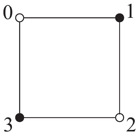
$B{H}_1$ and $B{H}_2$ are illustrated in Figure 1 and Figure 2, respectively.

Figure 1. $B{H}_1$.

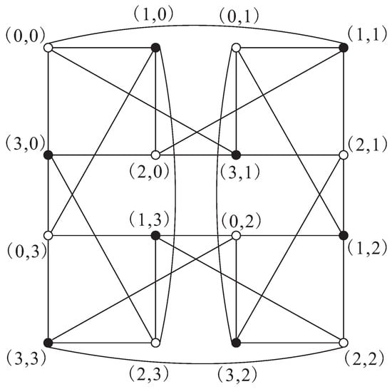
Figure 2. $B{H}_2$.

In the following, we give some basic properties of $B{H}_n$.

Proposition 1.

[10] The balanced hypercube is bipartite.

Proposition 2.

[10,20] The balanced hypercube is vertex-transitive and edge-transitive.

Proposition 3.

[10] The vertices $(a_0,a_1,\dots ,a_{n-1})$ and $((a_0+2)$ mod 4, $a_1,\dots ,a_{n-1})$ of $B{H}_n$ have the same neighborhood.

3. Main Results

Firstly, we characterize edges of the $B{H}_n$. Let u and v be two adjacent vertices in $B{H}_n$. If u and v differ in only the inner index, then $uv$ is said to be a 0-dimensional edge, and u is a 0-dimensional neighbor of v. If u and v differ in not only the inner index, but also some i-dimensional index ($i\ne 0$) of the vertices, then $uv$ is called an i-dimensional edge, and u is an i-dimensional neighbor of v. For convenience, we denote the set of all i-dimensional edges by $\partial D_i$ ($0\le i\le n-1$). Let $B{H}_{n-1}^{\left(i\right)}$ ($0\le i\le 3$) be the subgraph of $B{H}_n$ induced by the vertices of $B{H}_n$ with the $(n-1)$-dimensional index i. That is, the $B{H}_{n-1}^{\left(i\right)}$’s can be obtained from $B{H}_n$ by deleting all $(n-1)$-dimensional edges. Therefore, $B{H}_{n-1}^{\left(i\right)}\cong B{H}_{n-1}$ for each $0\le i\le 3$.

By Proposition 1, we know that $B{H}_n$ is bipartite. We can use $V_0$ and $V_1$ to denote the two partite sets of $B{H}_n$ such that $V_0$ and $V_1$ consist of vertices of $B{H}_n$ with an even inner index and an odd inner index, respectively. For convenience, the vertices of $V_0$ and $V_1$ are colored white and black, respectively. Throughout this paper, we use $w_i$ and $u_i$ (resp. $b_i$ and $v_i$) to denote white (resp. black) vertices in $B{H}_{n-1}^{\left(i\right)}$ ($i\in \{0,1,2,3\}$).

Lemma 1.

[16] In $B{H}_n$, $\partial D_i(0\le i\le n-1)$ can be divided into $4^{n-1}$ edge-disjoint 4-cycles for $n\ge 1$.

Lemma 2.

[12] The balanced hypercube $B{H}_n$ is Hamiltonian laceable and edge-bipancyclic for $n\ge 1$.

Lemma 3.

[17] The balanced hypercube $B{H}_n$ is hyper-Hamiltonian laceable for $n\ge 1$.

Lemma 4.

[30] Assume u and x are two different vertices in $V_0$, and v and y are two different vertices in $V_1$. Then, there exist two vertex-disjoint paths P and Q such that P joins x to y, Q joins u to v and $V\left(P\right)\cup V\left(Q\right)=V\left(B{H}_n\right)$, where $n\ge 1$.

Lemma 5.

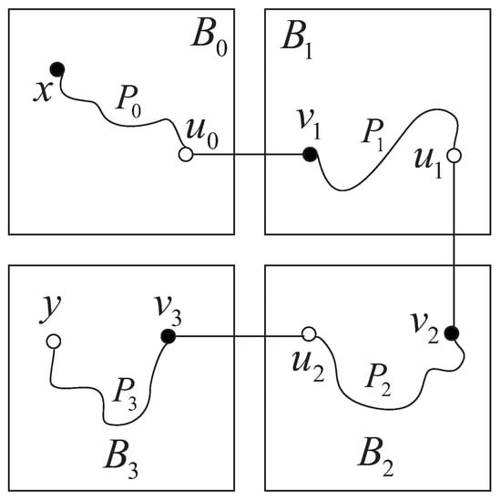
Let $n\ge 2$ be an integer. Suppose that $u,v,x$ and y are four distinct vertices differ only the inner index in $B{H}_n$. In addition, $u,x\in V_0$ and $v,y\in V_1$. Then, there exists a Hamiltonian path from u to v in $B{H}_n-x-y$.

Proof. 

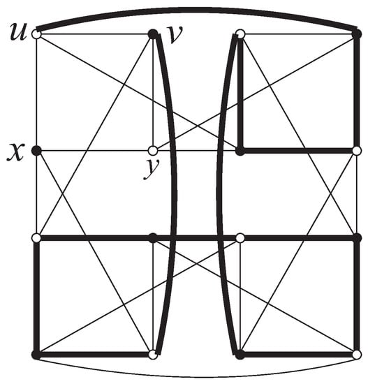
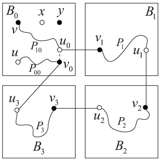
We proceed with the proof by the induction on n. First, we consider $n=2$. Clearly, $u,v,x$ and y are in the same 4-cycle of $\partial D_0$. A Hamiltonian path of $B{H}_2-x-y$ from u to v is shown in Figure 3. Thus, we suppose that the lemma holds for all integers $n-1$ with $n\ge 3$. Next, we consider $B{H}_n$. We split $B{H}_n$ into four $B{H}_{n-1}$s by deleting $(n-1)$-dimensional edges. For convenience, we denote the four $B{H}_{n-1}$s by $B_0$, $B_1$, $B_2$ and $B_3$ according to the last position of vertices in $B{H}_n$, respectively. Without loss of generality, we may assume that $u,v,x$ and y are in $B_0$. By an induction hypothesis, there exists a Hamiltonian path $P_0$ from u to v in $B_0-x-y$. Let $u_0{v}_0\in E\left(P_1\right)$, where $u_0$ (resp. $v_0$) are neither end-vertex of $P_0$. We denote the segment of $P_0$ from u to $v_0$ by $P_{00}$, and the segment of $P_0$ from $u_0$ to v by $P_{10}$. By Definition 1, $u_0$ (resp. $v_0$) has an $(n-1)$-dimensional neighbor $v_1$ (resp. $u_3$) in $B_1$ (resp. $B_3$). Moreover, there exist an edge $v_3{u}_2$ from $B_3$ to $B_2$, and an edge $v_2{u}_1$ from $B_2$ to $B_1$. Therefore, there exist a Hamiltonian path $P_3$ from $u_3$ to $v_3$ in $B_3$, a Hamiltonian path $P_2$ from $u_2$ to $v_2$ in $B_2$, and a Hamiltonian path $P_1$ from $u_1$ to $v_1$ of $B_1$. Hence, $⟨u,P_{00},v_0,u_3,P_3,v_3,u_2,P_2,v_2,u_1,P_1,v_1,u_0,P_{10},v⟩$ is a Hamiltonian path of $B{H}_n-x-y$ (see Figure 4). ☐

Figure 3. A Hamiltonian path of $B{H}_2-x-y$.

Figure 4. A Hamiltonian path of $B{H}_n-x-y$.

Next, we present the following lemma as a basis of our main theorem.

Lemma 6.

Let e be an arbitrary edge in $B{H}_2$. In addition, let $x\in V_1$ and $y\in V_0$ be any two vertices in $B{H}_2$ with $e\ne xy$. Then, there exists a Hamiltonian path between x and y passing through e.

Proof. 

By Proposition 2, $B{H}_2$ is vertex-transitive and edge-transitive, and we may suppose that $e=(0,0)(1,0)$. Obviously, if $e=xy$, then there exists no Hamiltonian path of $B{H}_2$ from x to y passing e. Thus, at most, one of x and y is the end-vertex of e. We consider the following two cases:

Case 1:

Neither x nor y is incident to e. By the relative positions of x and y, and Proposition 3, we consider the following: (1) $x\in V\left(B_0\right)$, $y\in V\left(B_0\right)$; (2) $x\in V\left(B_0\right)$, $y\in V\left(B_1\right)$; (3) $x\in V\left(B_0\right)$, $y\in V\left(B_2\right)$; (4) $x\in V\left(B_0\right)$, $y\in V\left(B_3\right)$; (5) $x\in V\left(B_1\right)$, $y\in V\left(B_1\right)$; (6) $x\in V\left(B_1\right)$, $y\in V\left(B_2\right)$; (7) $x\in V\left(B_1\right)$, $y\in V\left(B_3\right)$; (8) $x\in V\left(B_2\right)$, $y\in V\left(B_2\right)$; (9) $x\in V\left(B_2\right)$, $y\in V\left(B_3\right)$; (10) $x\in V\left(B_3\right)$, $y\in V\left(B_3\right)$. For simplicity, we list all Hamiltonian paths of the conditions above in Table 1.

Table 1. Hamiltonian paths passing through e with neither x nor y being incident to e.

	x	y	Hamiltonian Paths Passing through e with Neither x nor y Being Incident to e
(1)	(3,0)	(2,0)	(3,0)(0,3)(3,3)(2,3)(1,3)(0,2)(3,2)(2,2)(1,2)(2,1)(3,1)(0,1)(1,1)(0,0)(1,0)(2,0)
(2)	(3,0)	(0,1)	(3,0)(0,0)(1,0)(2,3)(3,3)(0,3)(1,3)(0,2)(3,2)(2,2)(1,2)(2,1)(3,1)(2,0)(1,1)(0,1)
(3)	(3,0)	(2,2)	(3,0)(0,3)(3,3)(2,3)(1,0)(0,0)(3,1)(2,0)(1,1)(0,1)(1,2)(2,1)(3,2)(0,2)(1,3)(2,2)
(4)	(3,0)	(0,3)	(3,0)(0,0)(1,0)(2,0)(3,1)(0,1)(1,1)(2,1)(1,2)(2,2)(3,2)(0,2)(1,3)(2,3)(3,3)(0,3)
(5)	(1,1)	(2,1)	(1,1)(0,1)(3,1)(2,0)(1,0)(0,0)(3,0)(0,3)(3,3)(2,3)(1,3)(0,2)(3,2)(2,2)(1,2)(2,1)
(6)	(1,1)	(2,2)	(1,1)(0,1)(3,1)(2,0)(1,0)(0,0)(3,0)(0,3)(3,3)(2,3)(1,3)(0,2)(3,2)(2,1)(1,2)(2,2)
(7)	(1,1)	(2,3)	(1,1)(0,0)(3,1)(0,1)(1,2)(2,1)(3,2)(2,2)(1,3)(0,2)(3,3)(0,3)(1,0)(2,0)(3,0)(2,3)
(8)	(1,2)	(2,2)	(1,2)(2,1)(1,1)(0,1)(3,1)(2,0)(1,0)(0,0)(3,0)(0,3)(3,3)(2,3)(1,3)(0,2)(3,2)(2,2)
(9)	(1,2)	(2,3)	(1,2)(2,1)(1,1)(0,1)(3,1)(2,0)(1,0)(0,0)(3,0)(0,3)(1,3)(2,2)(3,2)(0,2)(3,3)(2,3)
(10)	(1,3)	(2,3)	(1,3)(0,3)(3,0)(0,0)(1,0)(2,0)(1,1)(2,1)(3,1)(0,1)(3,2)(2,2)(1,2)(0,2)(3,3)(2,3)

Case 2:

Either x or y is incident to e. Without loss of generality, suppose that x is incident to e, that is, $x=(1,0)$. By Proposition 3, we need only to consider four conditions of y: (1) $y\in V\left(B_0\right)$; (2) $y\in V\left(B_1\right)$; (3) $y\in V\left(B_2\right)$; and (4) $y\in V\left(B_3\right)$. Again, we list Hamiltonian paths of the conditions of x and y in this case in Table 2. ☐

Table 2. Hamiltonian paths passing through e with x or y being incident to e.

	x	y	Hamiltonian Paths Passing through e with x or y Being Incident to e
(1)	(1,0)	(2,0)	(1,0)(0,0)(3,0)(0,3)(3,3)(2,3)(1,3)(0,2)(3,2)(2,2)(1,2)(2,1)(1,1)(0,1)(3,1)(2,0)
(2)	(1,0)	(0,1)	(1,0)(0,0)(3,0)(0,3)(3,3)(2,3)(1,3)(0,2)(3,2)(2,2)(1,2)(2,1)(1,1)(2,0)(3,1)(0,1)
(3)	(1,0)	(0,2)	(1,0)(0,0)(3,0)(0,3)(1,3)(2,3)(3,3)(2,2)(3,2)(2,1)(1,1)(2,0)(3,1)(0,1)(1,2)(0,2)
(4)	(1,0)	(0,3)	(1,0)(0,0)(3,0)(2,0)(3,1)(0,1)(1,1)(2,1)(1,2)(2,2)(3,2)(0,2)(1,3)(2,3)(3,3)(0,3)

Now, we are ready to state the main theorem of this paper.

Theorem 1.

Let $n\ge 2$ be an integer and e be an arbitrary edge in $B{H}_n$. In addition, let $x\in V_1$ and $y\in V_0$ be any two vertices in $B{H}_n$ with $e\ne xy$. Then, there exists a Hamiltonian path of $B{H}_n$ between x and y passing through e.

Proof. 

We prove this theorem by induction on n. By Lemma 6, we know that the theorem is true for $n=2$. Therefore, we suppose that the theorem holds for $n-1$ with $n\ge 3$. Next, we consider $B{H}_n$. Firstly, we divide $B{H}_n$ into $B{H}_{n-1}^{\left(i\right)}$ ($0\le i\le 3$) by deleting all $(n-1)$-dimensional edges. For convenience, we denote $B{H}_{n-1}^{\left(i\right)}$ by $B_i$ according to the last position of the vertices in $B{H}_n$ for each $i\in \{0,1,2,3\}$. Similarly, suppose that $e\in E\left(B_0\right)$. Let $x\in V_1$ and $y\in V_0$ be two distinct vertices in $B{H}_n$. By relative positions of x and y, we consider the following cases:

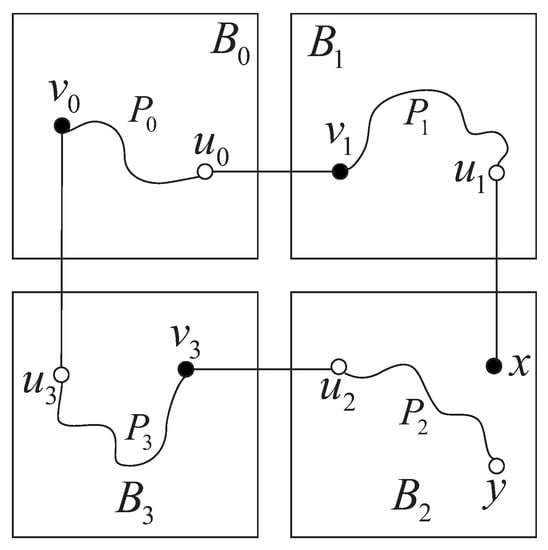
Case 1:

$x\in V\left(B_0\right)$, $y\in V\left(B_0\right)$. By an induction hypothesis, there exists a Hamiltonian path $P_0$ from x to y of $B_0$ passing through e. Thus, there is an edge $u_0{v}_0$ on $P_0$ such that $u_0{v}_0$ is not adjacent to e and $u_0{v}_0$ divides $P_0$ into two sections $P_{00}$ and $P_{10}$, where $P_{00}$ connects x to $u_0$ and $P_{10}$ connects $v_0$ to y. Let $v_1$ (resp. $u_3$) be an ($n-1$)-dimensional neighbor of $u_0$ (resp. $v_0$). By Definition 1, there exist an edge $u_1{v}_2$ from $B_1$ to $B_2$, and an edge $u_2{v}_3$ from $B_2$ to $B_3$. Thus, by Lemma 2, there exist a Hamiltonian path $P_1$ from $v_1$ to $u_1$ in $B_1$, a Hamiltonian path $P_2$ from $v_2$ to $u_2$ in $B_2$, and a Hamiltonian path $P_3$ from $v_3$ to $u_3$ in $B_3$. Hence, $⟨x,P_{00},u_0,v_1,P_1,u_1,v_2,P_2,u_2,v_3,P_3,u_3,v_0,P_{10},y⟩$ is a Hamiltonian path of $B{H}_n$ from x to y passing through e (see Figure 5).

Figure 5. Illustration for Case 1.

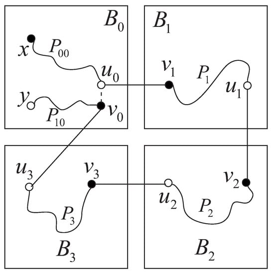
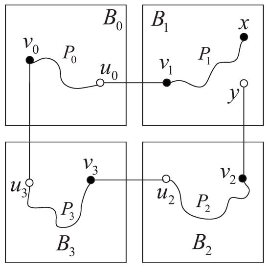
Case 2:

$x\in V\left(B_0\right)$, $y\in V\left(B_1\right)$. Let $u_0\in V\left(B_0\right)$ be a white vertex such that $u_0$ is not incident to e. By an induction hypothesis, there exists a Hamiltonian path $P_0$ of $B_0$ from x to $u_0$ passing through e. Supposing that $v_0$ is a black vertex adjacent to $u_0$ on $P_0$, we denote the segment of the path $P_0$ from x to $v_0$ by $P_{00}$. Let the two $(n-1)$-dimensional neighbors of $u_0$ be $b_1$ and $v_1$. By Lemma 2, there exists a Hamiltonian path $P_1$ of $B_1$ from $b_1$ to y. Let $u_1$ be the neighbor of $v_1$ in the section of $P_1$ from $b_1$ to $v_1$. Then $P_1-u_1{v}_1$ consists of two subpaths $P_{01}$ and $P_{11}$, which connect $u_1$ to $b_1$ and $v_1$ to y, respectively. Let $u_3$ (resp. $v_2$) be an ($n-1$)-dimensional neighbor of $v_0$ (resp. $u_1$). Furthermore, there exists an edge $v_3{u}_2$ from $B_3$ to $B_2$. Then, there exist a Hamiltonian path $P_2$ from $u_2$ to $v_2$ in $B_2$, and a Hamiltonian path $P_3$ from $u_3$ to $v_3$ in $B_3$. Hence, $⟨x,P_{00},v_0,u_3,P_3,v_3,u_2,P_2,v_2,u_1,P_{01},b_1,u_0,v_1,P_{11},y⟩$ is a Hamiltonian path of $B{H}_n$ from x to y passing through e (see Figure 6).

Figure 6. Illustration for Case 2.

Case 3:

$x\in V\left(B_0\right)$, $y\in V\left(B_2\right)$. Let $u_0$ be a white vertex in $B_0$ not incident to e, and $b_1$ and $v_1$ be two $(n-1)$-dimensional neighbors of $u_0$. In addition, assume that $w_1$ is an arbitrary white vertex in $B_1$. There exists a Hamiltonian path of $B_1$ from $b_1$ to $w_1$. Thus, there exists an edge $u_1{v}_1\in E\left(P_1\right)$ whose removal will lead to two disjoint subpaths $P_{01}$ and $P_{11}$, where $P_{01}$ connects $u_1$ to $b_1$ and $P_{11}$ connects $v_1$ to $w_1$. Let $v_2$ (resp. $b_2$) be an $(n-1)$-dimensional neighbor of $u_1$ (resp. $w_1$). There also exists a Hamiltonian path $P_2$ of $B_2$ from y to $b_2$ via the edge $v_2{u}_2$. Deleting $v_2{u}_2$ results in two disjoint paths $P_{02}$ and $P_{12}$, where $P_{02}$ connects $u_2$ to $b_2$ and $P_{12}$ connects $v_2$ to y. By an induction hypothesis, there exists a Hamiltonian path $P_0$ of $B_0$ from x to $u_0$ via the edge $v_0{u}_0$. For convenience, denote $P_0-u_0$ by $P_{00}$, that is, $P_{00}$ connects x to $v_0$. Let $u_3$ (resp. $v_3$) be an $(n-1)$-dimensional neighbor of $v_0$ (resp. $u_2$). Again, there exists a Hamiltonian path $P_3$ of $B_3$ from $u_3$ to $v_3$. Hence, $⟨x,P_{00},v_0,u_3,P_3,v_3,u_2,P_{02},b_2,w_1,P_{11},v_1,u_0,b_1,P_{01},u_1,v_2,P_{12},y⟩$ is a Hamiltonian path of $B{H}_n$ from x to y passing through e (see Figure 7).

Figure 7. Illustration for Case 3.

Case 4:

$x\in V\left(B_0\right)$, $y\in V\left(B_3\right)$. Let $u_0$ (resp. $v_3$) be a white (resp. black) vertex in $B_0$ (resp. $B_3$). There exist an edge $u_0{v}_1$ from $B_0$ to $B_1$, an edge $u_1{v}_2$ from $B_1$ to $B_2$, and an edge $u_2{v}_3$ from $B_2$ to $B_3$. By Lemma 2, there exist a Hamiltonian path $P_1$ of $B_1$ from $v_1$ to $u_1$, a Hamiltonian path $P_2$ of $B_2$ from $v_2$ to $u_2$, and a Hamiltonian path $P_3$ of $B_3$ from $v_3$ to $u_3$. By an induction hypothesis, there exists a Hamiltonian path $P_0$ of $B_0$ from x to $u_0$ passing through e. Hence, $⟨x,P_0,u_0,v_1,P_1,u_1,v_2,P_2,u_2,v_3,P_3,y⟩$ is a Hamiltonian path of $B{H}_n$ from x to y passing through e (see Figure 8).

Figure 8. Illustration for Case 4.

Case 5:

$x\in V\left(B_1\right)$, $y\in V\left(B_1\right)$. Let $v_1\ne x$ be a black vertex in $B_1$. By Lemma 3, there exists a Hamiltonian path $P_1$ of $B_1-y$ from x to $v_1$. Furthermore, there exist an edge $v_1{u}_0$ from $B_1$ to $B_0$, an edge $v_0{u}_3$ from $B_0$ to $B_3$, an edge $v_3{u}_2$ from $B_3$ to $B_2$, and an edge $v_{2}y$ from $B_2$ to $B_1$. Moreover, there exist a Hamiltonian path $P_0$ of $B_0$ from $u_0$ to $v_0$ passing through e, a Hamiltonian path $P_3$ of $B_3$ from $u_3$ to $v_3$, and a Hamiltonian path $P_2$ of $B_2$ from $u_2$ to $v_2$. Hence, $⟨x,P_1,v_1,u_0,P_0,v_0,u_3,P_3,v_3,u_2,P_2,v_2,y⟩$ is a Hamiltonian path of $B{H}_n$ from x to y passing through e (see Figure 9).

Figure 9. Illustration for Case 5.

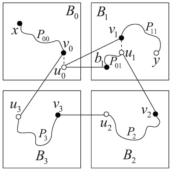
Case 6:

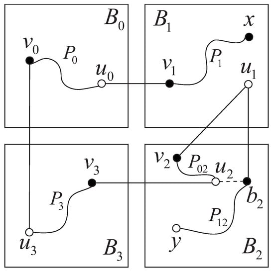
$x\in V\left(B_1\right)$, $y\in V\left(B_2\right)$. Let $v_1\ne x$ (resp. $u_1$) be a black (resp. white) vertex in $B_1$. By Lemma 3, there exists a Hamiltonian path $P_1$ of $B_1-u_1$ from x to $v_1$. In addition, suppose that $v_2$ and $b_2$ are two $(n-1)$-dimensional neighbors of $u_1$. By Lemma 2, there exists a Hamiltonian $P_2$ of $B_2$ from $v_2$ to y via the edge $u_2{b}_2$. Thus, $P_2$ can be divided into three sections: $P_{02}$, $u_2{v}_2$ and $P_{12}$, where $P_{02}$ connects $u_2$ to $v_2$ and $P_{12}$ connects $b_2$ to y. Furthermore, there exist an edge $v_1{u}_0$ from $B_1$ to $B_0$, an edge $v_0{u}_3$ from $B_0$ to $B_3$, and an edge $v_3{u}_2$ from $B_3$ to $B_2$. Therefore, there exist a Hamiltonian path $P_0$ of $B_0$ from $u_0$ to $v_0$ passing through e, and a Hamiltonian path $P_3$ of $B_3$ from $u_3$ to $v_3$. Hence, $⟨x,P_1,v_1,u_0,P_0,v_0,u_3,P_3,v_3,u_2,P_{02},v_2,u_1,b_2,P_{12},y⟩$ is a Hamiltonian path of $B{H}_n$ from x to y passing through e (see Figure 10).

Figure 10. Illustration for Case 6.

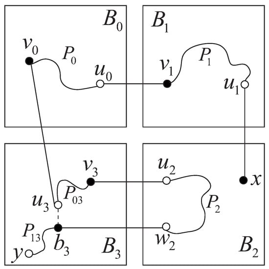
Case 7:

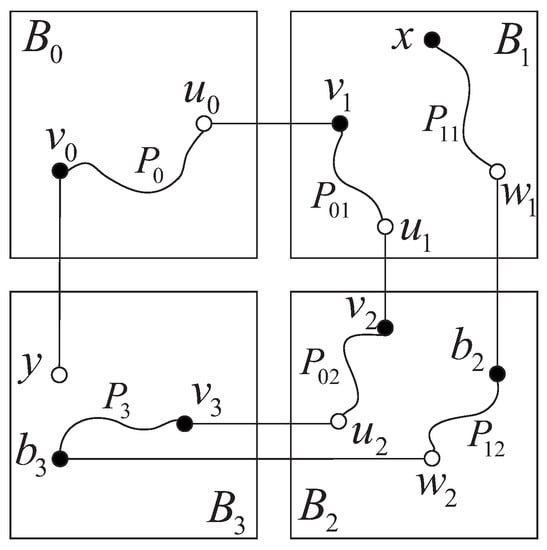
$x\in V\left(B_1\right)$, $y\in V\left(B_3\right)$. Let $v_3$ and $b_3$ be two black vertices in $B_3$. Suppose that $u_2$ and $w_2$ are $(n-1)$-dimensional neighbors of $v_2$ and $b_2$, respectively. By Lemma 3, there exists a Hamiltonian path $P_3$ of $B_3-y$ from $b_3$ to $v_3$. By Definition 1, there exist two edges $v_2{u}_1$ and $b_2{w}_1$ from $B_2$ to $B_1$, an edge $v_1{u}_0$ from $B_1$ to $B_0$, and an edge $v_{0}y$ from $B_0$ to $B_3$, where $x\ne v_1$. By Lemma 4, there exist two vertex-disjoint paths $P_{01}$ and $P_{11}$ such that $P_{01}$ joins $v_1$ and $u_1$, $P_{11}$ joins x and $w_1$, and $V\left(P_{01}\right)\cup V\left(P_{11}\right)=V\left(B_1\right)$. Similarly, there exist two vertex-disjoint paths $P_{02}$ and $P_{12}$ such that $P_{02}$ joins $v_2$ and $u_2$, $P_{12}$ joins $b_2$ and $w_2$, and $V\left(P_{02}\right)\cup V\left(P_{12}\right)=V\left(B_2\right)$. By an induction hypothesis, there exists a Hamiltonian path $P_0$ of $B_0$ from $u_0$ to $v_0$ passing through e. Hence, $⟨x,P_{11},w_1,b_2,P_{12},w_2,b_3,P_3,v_3,u_2,P_{02},v_2,u_1,P_{01},v_1,u_0,P_0,v_0,y⟩$ is a Hamiltonian path of $B{H}_n$ from x to y passing through e (see Figure 11).

Figure 11. Illustration for Case 7.

Case 8:

$x\in V\left(B_2\right)$, $y\in V\left(B_2\right)$. Let $u_2\in V\left(B_2\right)$ be an arbitrary white vertex. By Lemma 3, there exists a Hamiltonian path $P_2$ of $B_2-x$ from $u_2$ to y. By Definition 1, there exist an edge $x{u}_1$ from $B_2$ to $B_1$, an edge $v_1{u}_0$ from $B_1$ to $B_0$, an edge $v_0{u}_3$ from $B_0$ to $B_3$, and an edge $v_3{u}_2$ from $B_3$ to $B_2$. Following Lemma 2, we can obtain a Hamiltonian path $P_1$ of $B_1$ from $u_1$ to $v_1$, and a Hamiltonian path $P_3$ of $B_3$ from $u_3$ to $v_3$. By an induction hypothesis, there exists a Hamiltonian path $P_0$ of $B_0$ from $u_0$ to $v_0$ passing through e. Therefore, $⟨x,u_1,P_1,v_1,u_0,P_0,v_0,u_3,P_3,v_3,u_2,P_2,y⟩$ is a Hamiltonian path of $B{H}_n$ from x to y passing through e (see Figure 12).

Figure 12. Illustration for Case 8.

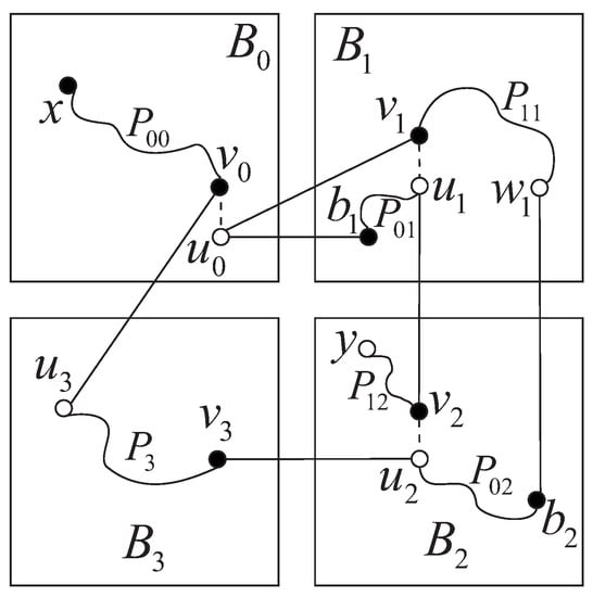
Case 9:

$x\in V\left(B_2\right)$, $y\in V\left(B_3\right)$. Let $u_2$ and $w_2$ be two distinct white vertices in $B_2$, and $v_3$ and $b_3$ be $(n-1)$-dimensional neighbors of $u_2$ and $w_2$, respectively. By Lemma 3, there exists a Hamiltonian path $P_2$ of $B_2-x$ from $u_2$ to $w_2$. By Lemma 2, there exists a Hamiltonian path $P_3$ of $B_3$ from $v_3$ to y via the edge $u_3{b}_3$. By deleting $u_3{b}_3$, we can obtain two disjoint subpaths: $P_{03}$ and $P_{13}$, where $P_{03}$ connects $u_3$ to $v_3$ and $P_{13}$ connects $b_3$ to y. Furthermore, there exist an edge $x{u}_1$ from $B_2$ to $B_1$, an edge $v_1{u}_0$ from $B_1$ to $B_0$, and an edge $v_0{u}_3$ from $B_0$ to $B_3$. By Lemma 2, there exists a Hamiltonian path $P_1$ of $B_1$ from $u_1$ to $v_1$. By an induction hypothesis, there exists a Hamiltonian path $P_0$ of $B_0$ from $u_0$ to $v_0$ passing through e. Hence, $⟨x,u_1,P_1,v_1,u_0,P_0,v_0,u_3,P_{03},v_3,u_2,P_2,w_2,b_3,P_{13},y⟩$ is a Hamiltonian path of $B{H}_n$ from x to y passing through e (see Figure 13).

Figure 13. Illustration for Case 9.

Case 10:

$x\in V\left(B_3\right)$, $y\in V\left(B_3\right)$. The proof is analogous to that of Case 5, and we omit it. ☐

4. Conclusions

In this paper, we study a type of path embedding of the balanced hypercube, and show that, for an arbitrary edge $e\ne xy$, there exists a Hamiltonian path between any two vertices x and y in different partite sets passing through e. This result also implies that each edge is on a Hamiltonian cycle of the balanced hypercube, which is part of the results of edge bipancyclicity of the balanced hypercube.

References

- Abraham, S.; Padmanabhan, K. The twisted cube topology for multiprocessors: A study in network asymmetry. J. Parall. Distrib. Comput. 1991, 13, 104–110. [Google Scholar] [CrossRef]
- Choudum, S.A.; Sunitha, V. Augmented cubes. Networks 2002, 40, 71–84. [Google Scholar] [CrossRef]
- Cull, P.; Larson, S.M. The Möbius cubes. IEEE Trans. Comput. 1995, 44, 647–659. [Google Scholar] [CrossRef]
- Dally, W.J. Performance analysis of k-ary n-cube interconnection networks. IEEE Trans. Comput. 1990, 39, 775–785. [Google Scholar] [CrossRef]
- Efe, K. The crossed cube architecture for parallel computation. IEEE Trans. Parall. Distr. Syst. 1992, 3, 513–524. [Google Scholar] [CrossRef]
- El-amawy, A.; Latifi, S. Properties and performance of folded hypercubes. IEEE Trans. Parall. Distrib. Syst. 1991, 2, 31–42. [Google Scholar] [CrossRef]
- Li, T.K.; Tan, J.J.M.; Hsu, L.H.; Sung, T.Y. The shuffle-cubes and their generalization. Inform. Process. Lett. 2001, 77, 35–41. [Google Scholar] [CrossRef]
- Preparata, F.P.; Vuillemin, J. The cube-connected cycles: A versatile network for parallel computation. Comput. Arch. Syst. 1981, 24, 300–309. [Google Scholar] [CrossRef]
- Xiang, Y.; Stewart, I.A. Augmented k-ary n-cubes. Inform. Sci. 2011, 181, 239–256. [Google Scholar] [CrossRef]
- Wu, J.; Huang, K. The balanced hypercube: A cube-based system for fault-tolerant applications. IEEE Trans. Comput. 1997, 46, 484–490. [Google Scholar]
- Huang, K.; Wu, J. Fault-tolerant resource placement in balanced hypercubes. Inform. Sci. 1997, 99, 159–172. [Google Scholar] [CrossRef]
- Xu, M.; Hu, H.; Xu, J. Edge-pancyclicity and Hamiltonian laceability of the balanced hypercubes. Appl. Math. Comput. 2007, 189, 1393–1401. [Google Scholar] [CrossRef]
- Yang, M. Bipanconnectivity of balanced hypercubes. Comput. Math. Appl. 2010, 60, 1859–1867. [Google Scholar] [CrossRef]
- Huang, K.; Wu, J. Area efficient layout of balanced hypercubes. Int. J. High Speed Electr. Syst. 1995, 6, 631–645. [Google Scholar] [CrossRef]
- Yang, M. Super connectivity of balanced hypercubes. Appl. Math. Comput. 2012, 219, 970–975. [Google Scholar] [CrossRef]
- Lü, H.; Li, X.; Zhang, H. Matching preclusion for balanced hypercubes. Theor. Comput. Sci. 2012, 465, 10–20. [Google Scholar] [CrossRef]
- Lü, H.; Zhang, H. Hyper-Hamiltonian laceability of balanced hypercubes. J. Supercomput. 2014, 68, 302–314. [Google Scholar] [CrossRef]
- Lü, H.; Gao, X.; Yang, X. Matching extendability of balanced hypercubes. Ars Combinatoria 2016, 129, 261–274. [Google Scholar]
- Lü, H. On extra connectivity and extra edge-connectivity of balanced hypercubes. Int. J. Comput. Math. 2017, 94, 813–820. [Google Scholar] [CrossRef]
- Zhou, J.-X.; Wu, Z.-L.; Yang, S.-C.; Yuan, K.-W. Symmetric property and reliability of balanced hypercube. IEEE Trans. Comput. 2015, 64, 876–881. [Google Scholar] [CrossRef]
- Zhou, J.-X.; Kwak, J.; Feng, Y.-Q.; Wu, Z.-L. Automorphism group of the balanced hypercube. Ars Math. Contemp. 2017, 12, 145–154. [Google Scholar]
- Jha, P.K.; Prasad, R. Hamiltonian decomposition of the rectangular twisted torus. IEEE Trans. Comput. 2012, 23, 1504–1507. [Google Scholar] [CrossRef]
- Chang, N.-W.; Tsai, C.-Y.; Hsieh, S.-Y. On 3-extra connectivity and 3-extra edge connectivity of folded hypercubes. IEEE Trans. Comput. 2014, 63, 1594–1600. [Google Scholar] [CrossRef]
- Hsieh, S.-Y.; Yu, P.-Y. Fault-free mutually independent Hamiltonian cycles in hypercubes with faulty edges. J. Combin. Optim. 2007, 13, 153–162. [Google Scholar] [CrossRef]
- Park, C.; Chwa, K. Hamiltonian properties on the class of hypercube-like networks. Inform. Process. Lett. 2004, 91, 11–17. [Google Scholar] [CrossRef]
- Wang, S.; Li, J.; Wang, R. Hamiltonian paths and cycles with prescribed edges in the 3-ary n-cube. Inform. Sci. 2011, 181, 3054–3065. [Google Scholar] [CrossRef]
- Simmons, G. Almost all n-dimensional rectangular lattices are Hamilton–Laceable. Congr. Numer. 1978, 21, 103–108. [Google Scholar]
- West, D.B. Introduction to Graph Theory, 2nd ed.; Prentice Hall: Englewood Cliffs, NJ, USA, 2001. [Google Scholar]
- Xu, J.M. Topological Structure and Analysis of Interconnection Networks; Kluwer Academic Publishers: Dordrecht, The Netherlands, 2001. [Google Scholar]
- Cheng, D.; Hao, R.-X.; Feng, Y.-Q. Two node-disjoint paths in balanced hypercubes. Appl. Math. Comput. 2014, 242, 127–142. [Google Scholar] [CrossRef]
© 2017 by the authors. Licensee MDPI, Basel, Switzerland. This article is an open access article distributed under the terms and conditions of the Creative Commons Attribution (CC BY) license (http://creativecommons.org/licenses/by/4.0/).