Abstract
Nowadays, the increasing demands of location-based services (LBS) have spurred the rapid development of indoor positioning systems (IPS). However, the performance of IPSs is affected by the fluctuation of the measured signal. In this study, a Gaussian filtering algorithm based on an extreme learning machine (ELM) is proposed to address the problem of inaccurate indoor positioning when significant Received Signal Strength Indication (RSSI) fluctuations happen during the measurement process. The Gaussian filtering method is analyzed and compared, which can effectively filter out the fluctuant signals that were caused by the environment effects in an RFID-based positioning system. Meanwhile, the fast learning ability of the proposed ELM algorithm can reduce the time consumption for the offline and online service, and establishes the network positioning regression model between the signal strengths of the tags and their corresponding positions. The proposed positioning system is tested in a real experimental environment. In addition, system test results demonstrate that the positioning algorithms can not only provide higher positioning accuracy, but also achieve a faster computational efficiency compared with other previous algorithms.
1. Introduction
Indoor positioning systems (IPS) are emerging as a technology, due to the increasing popularity and demand in location based service indoors [1,2]. One of the most famous location-aware services is the Global Positioning System (GPS), but there must be a direct line-of-sight between receiver and satellite in an unshielded environment. GPS is used for outdoor locations. However, its performance is very poor in indoor environments [3]. Therefore, different types of indoor positioning systems have been developed for personal and commercial needs [4,5]. Among all of the indoor positioning methods, Benavente-Peces et al. [6] found that Radio Frequency Identification (RFID) is the best choice for indoor positioning with high accuracy and low cost.
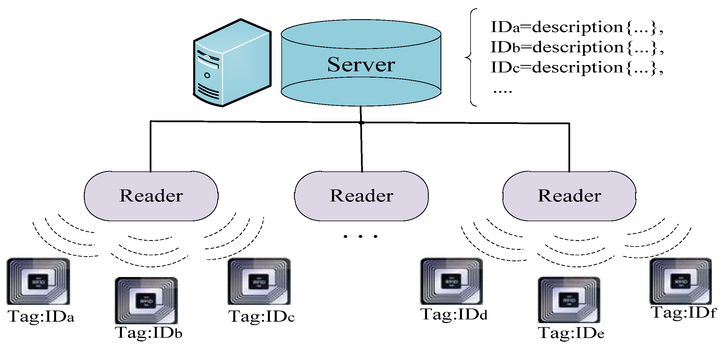
RFID is a rapidly developing technology that it uses radio frequency (RF) signals to automatically identify objects. It has been widely applied in various fields for tool tracking, process management, access control and supply chain, such as access cards and electronic wallets. A typical RFID networks system was illustrated in Figure 1 that consists of three different entities: RFID readers, tags and servers. Furthermore, the RFID system has also been applied in the location field for the real-time tracking and positioning of indoor targets. At first, Shiraishi et al. [7] proposed an indoor positioning estimation system based on UHF RFID. Furthermore, Wang et al. [8] have successfully designed an indoor personnel tracking and positioning system based on RFID technology combined with images. Similarly, Montaser et al. [9] present a low-cost indoor positioning and material tracking methodology for construction projects using passive UHF RFID technology. Goodrum et al. [10] also explored the applications of UHF RFID technology that is used for tool tracking on construction job sites. Therefore, UHF RFID is used for indoor positioning in this paper.
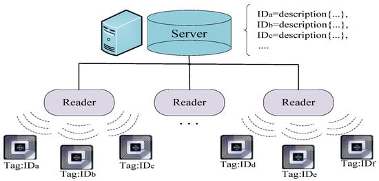
Figure 1.
Architecture of a rapidly RFID system.
Currently, an extensive body of research for the IPS has focused on the machine learning approaches such as Extreme Learning Machine (ELM) [11], Artificial Neural Network (ANN) or Support Vector Machine (SVM) [12] and so on, in order to overcome the shortcomings faced by the traditional positioning methods. Wu et al. [13] applied the ANN to overcome the limitations of the empirical positioning formula, which was used in the previous research. The ANN can learn the geography features to adapt to the real world, which can avoid the impact of the multipath phenomenon and be flexibly applied to any environment. However, the weights of ANN are not easy to be determined. For that reason, Kuo et al. [14] proposed a feature selection-based Back-Propagation (BP) neural network that uses an Artificial Immune System (AIS) (BP-AIS) to determine the connecting weights of ANN, and forecasts the position of the picking staff for warehouse management. Similarly, Ceravolo et al. [15] applied the genetic algorithm (GA) to determine the parameters of BP network (GA-BP) and applied it to predict and control the environment temperature.
In addition, Zou et al. [16] proposed the ELM to overcome the indoor positioning problem and, through the experimental evaluation, reported that an ELM-based on positioning system can provide higher positioning accuracy and robustness over that of a traditional method. Jiang et al. [17] presented a fusion position framework with a Particle Filter using Wi-Fi signals and motion sensors, which use the ELM regression algorithm to predict the location of the target. The system consists of three main modules: a sensor data based position model (ELM regression), the fusion Particle Filter model and the Wi-Fi based position model. The results show that the proposed method achieves a good performance, for example, achieving a better accuracy than the traditional fingerprint method. Fu et al. [18] proposed the kernel ELM to locate the target position and compared it with machine learning algorithms such as SVM [19,20] and BP, and the result reveals that the kernel ELM has good prediction performance and fast learning speed.
It is worth mentioning that the above research has been made good progress. Unfortunately, most of these studies have neglected the filtering processing for experimental data because the RSSI is affected by many factors, such as indoor temperature, humidity, multi-path effect and so on, which leads to a large fluctuation of RSSI. Therefore, this paper will propose an indoor positioning system based on a Gaussian filter combined with ELM and verify its performance via comparison with prevailing methods.
The remainder of this paper is organized as follows. Section 2 presents the related works of this research. The proposed method is explained in Section 3. Section 4 designed the experimental and comparison analysis. Section 5 discussed the experimental results. Finally, Section 6 presents the conclusions and future research directions.
2. Related Works
2.1. IPS Technologies
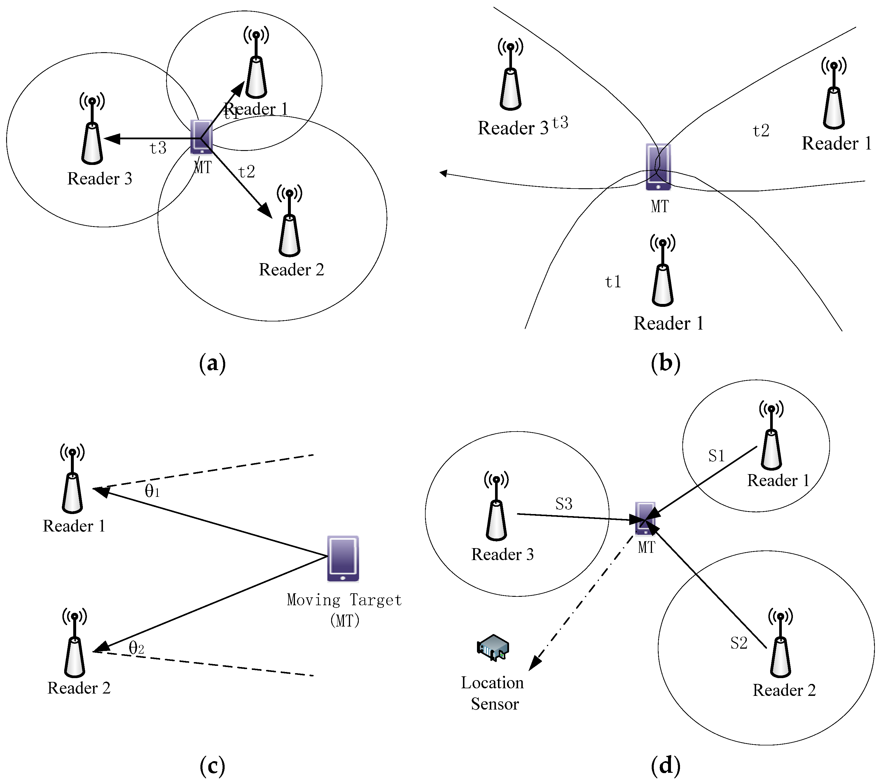
At present, there are four frequently used localization technologies based on the measurement of distances or angles between reference points: Time of Arrival (TOA), Time Difference of Arrival (TDOA), Angle of Arrival (AOA) [21] and Received Signal Strength Indication (RSSI) [22] are shown as Figure 2. Hatami et al. [23] describes in detail the performance differences for each location system. The TOA and TDOA based systems are more suitable for outdoor or large-scale open indoor environments, and the RSSI based system is the most suitable for tight indoor environments. Furthermore, Reference [24] has found that the positioning system based on the RSSI measurement has two main advantages: simple implementation and cost effectiveness. This study takes into account the technological problems and considerable costs, and the basic RSSI measurement method based on localization is adopted.
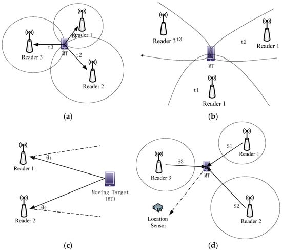
Figure 2.
Four measurement based positioning techniques: (a) TOA based estimation; (b) TDOA based estimation; (c) AOA based estimation; (d) RSSI based estimation.
2.2. ELM Algorithm
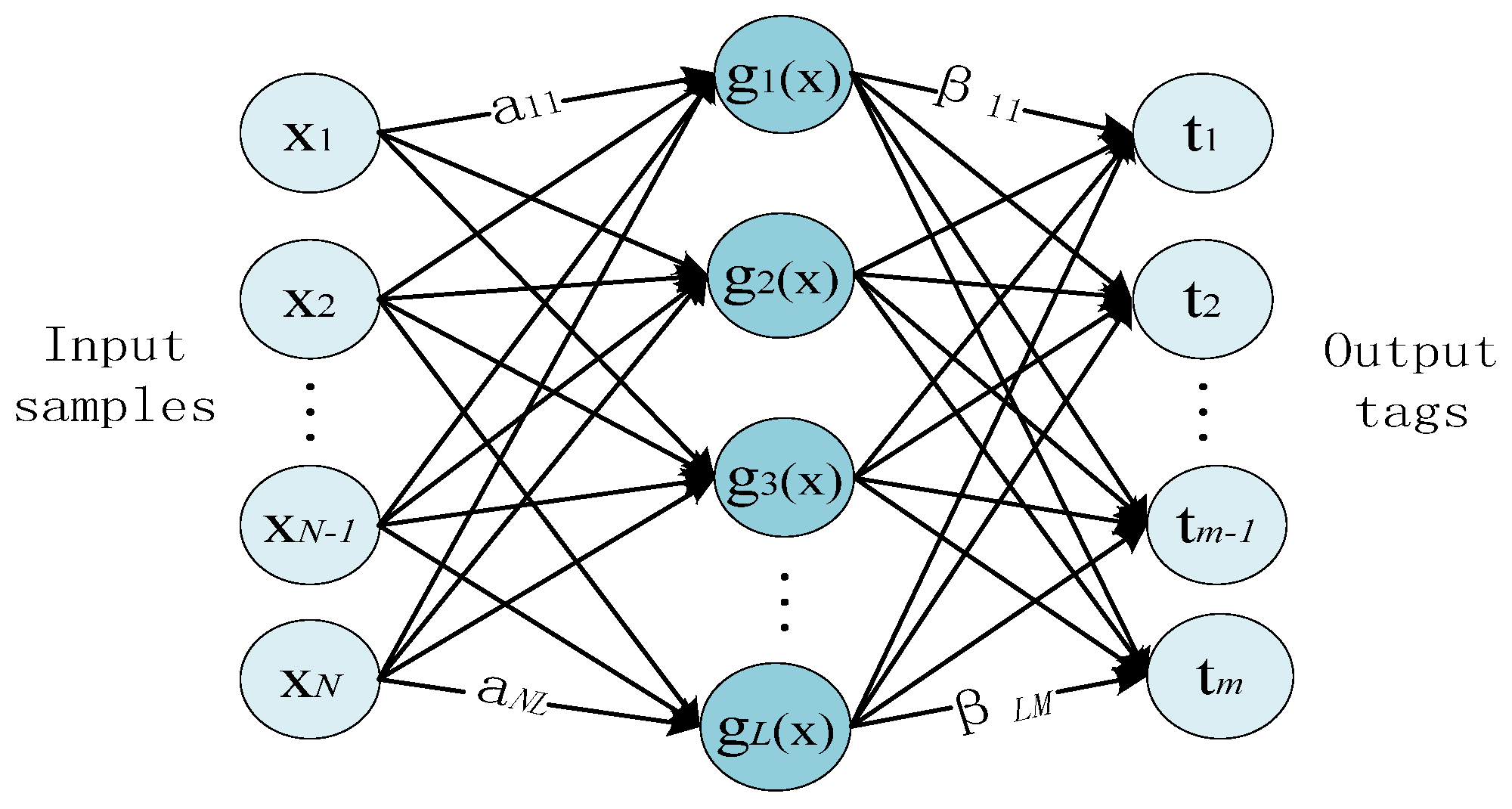
ELM [25] is a type of machine learning algorithm based on a single-hidden Layer Feed-forward neural Network (SLFN) architecture developed by Huang et al. It has been demonstrated that ELM can provide good generalization performance at an extremely fast learning speed [26,27]. Given , an arbitrary distinct training set , where is an input vector , and is an target vector . The goal of regression is to find the relationship between and . Since the only parameters to be optimized are the output weights, the training of ELM is equivalent to solving a least squares problem [28]. Figure 3 shows the typical network structure of the SLFN.
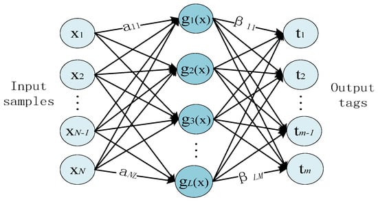
Figure 3.
The SLFN network structure with hidden neurons.
In the training process, the first stage is that maps the data from the -dimensional input space to the -dimensional hidden-layer feature space (ELM feature space)
where is the output of a row vector of the hidden layer, .
The mathematical model of the SLFNs can be summarized as Equation (2):
where is the hidden layer output matrix, is the output weight matrix and is the target vector
Each output of ELM is given by Equation (4)
ELM theory is to minimize the training error but also the smallest norm of the output weights [29]:
where is the penalty coefficient on the training errors, and is the training error vector of the output nodes with respect to the th training pattern .
3. The Proposed ELM Based IPS
3.1. Data Gaussian Filtering
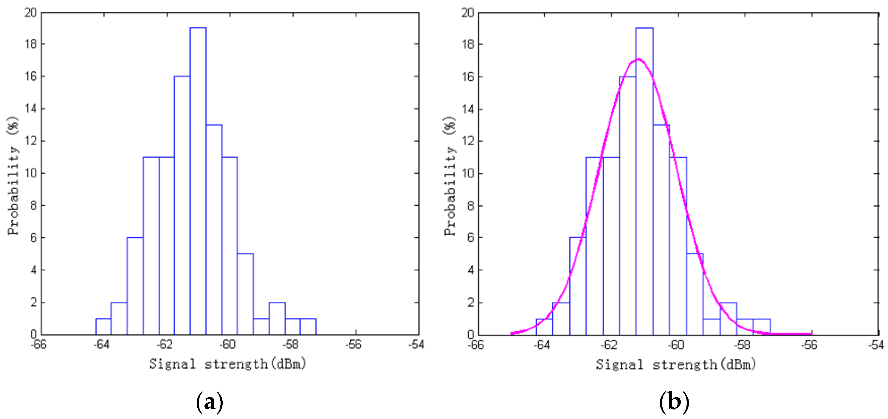
Data Gaussian filtering is used to reduce the signal fluctuation of RSSI, which is obtained by repeated measurements at the fixed position. Assuming that , where represents the RSSI measurement vector of the tag that contains RSSI values that are received by a number of readers , and the observed position of the tag is , is the number of reference tags. Defining that is the RSSI vector of the th tag that is measured by the reader at a fixed point , where is the number of measurements, and is the RSSI vector that is processed by the principle of Gaussian distribution. Figure 4a shows the repeated measurement results from a specified tag at a fixed point k. From Figure 4a, it can be seen that the changes in RSSI measurement can be approximated as a parametric distribution, and the Gaussian distribution fits the RSSI distribution from a fixed point (measured in dBm) as shown in Figure 4b.

Figure 4.
The RSSI data and Gaussian fitting: (a) The RSSI measurement values from a specified tag at a fixed point; (b) The PDF and Gaussian fitting for RSSI data.
Figure 4 implies that the can model the Gaussian distribution:
where is the expected value of RSSI and is the variance of RSSI, and is given by
According to the principle of Gaussian distribution, the small probability event of is excluded, and the data of is chosen as effective experimental data.
Since the signal strength values received from different locations of tags are independent, is still consistent with the Gaussian density distribution, and is given by:
where , , and is the number of remaining measured values, which has been processed by the principle of Gaussian distribution.
When the function value , the corresponding RSSI value has a high probability value; when , the corresponding RSSI value has a small probability value, as defined by:
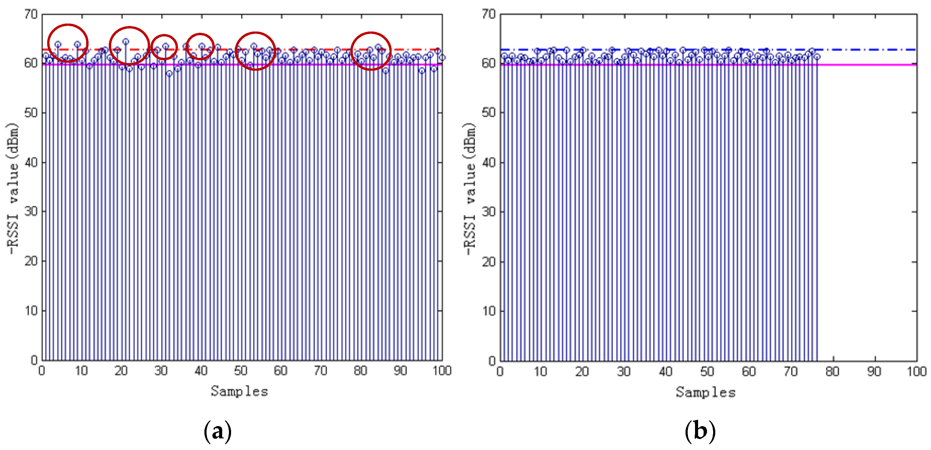
According to the general engineering practice that , and the effective interval of RSSI value is Equation (9). Figure 5 shows the RSSI value of a tag that is collected at a fixed point several times:

Figure 5.
The RSSI value of a tag that is collected at a fixed point for several times: (a) the RSSI values before Gaussian process; (b) the RSSI values after Gaussian process.
The final output of the Gaussian process is the arithmetic mean of all the RSSI values within the interval [, ], and is given by
where is a number that satisfies Equation (9).
3.2. ELM Learning Method
The proposed ELM method considers the localization problem as a regression problem. Suppose the given training data is , setting rank , where denotes the hidden output matrix. The ELM network with hidden nodes is shown in Figure 3, and the output function of this network can be expressed as follows:
where is the weight connecting the th hidden node to the output node, and are the learning parameters of hidden nodes, and is the output of the th hidden node.
For the additive hidden node, , , and if SLFNs with hidden nodes can approximate the samples with zero errors, there exist , , and such that
where , .
The ELM learning algorithm consists of three main procedures as shown in Figure 6.

Figure 6.
The learning of ELM algorithm.
Step1: Randomly assign the input parameters: input weights and biases ,
Step2: Calculate the initial hidden layer output matrix
Step3: Estimate the initial output weight . For , the problem is equivalent to minimizing , which can be written as
The optimal solution is given by , where is the Moore–Penrose generalized inverse of hidden layer output matrix .
3.3. Overall System
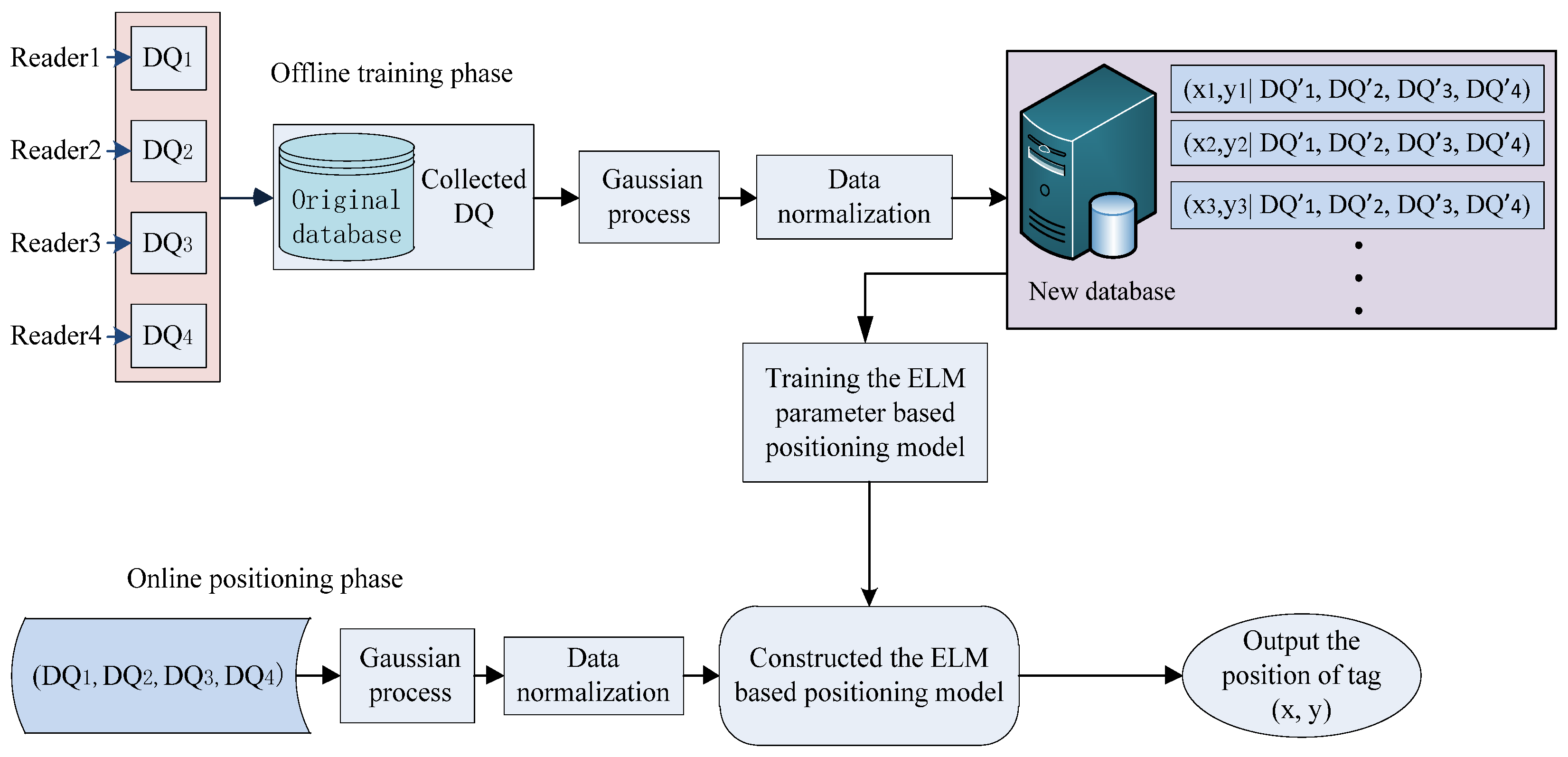
The framework of the proposed ELM with a Gaussian process for IPS is shown in Figure 7. It contains two localization phases: the offline phase and the online phase. During the offline phase, the collected RSSI of reference tags and their physical locations are adopted as training inputs and training targets, respectively. The cluster classification is conducted for all DQ values in the database through ELM learning to define the parameters of the network and establish an initial ELM regression model of environment characteristics for online positioning. During the online phase, the real-time DQ values will be fed into the trained ELM model, and, then, the estimated location will be calculated.

Figure 7.
The framework of ELM IPS based on Gaussian process.
The main task of ELM learning algorithm here is the cluster analysis for training sample sets which are stored in the RFID localization database. Defining , where is the coordinate of the th tag and its corresponding . In addition, at time , the reader repeatedly obtains the RSSI value of the tag at a fixed point , namely, is the acquired RSSI vector for tag that is measured by the th reader times. All are collected to build an original database. As discussed in Section 3.1, the RSSI value in the original database is processed by Gaussian filter to reduce the signal fluctuation that is caused by the indoor environment effects. Furthermore, in order to avoid the domination of large feature values, the datasets are normalized to the range of [0, 1] by using the corresponding maximum and minimum values.
The input training data sets in Figure 7 are , where represents the coordinates of the point to be measured, and represents its corresponding RSSI values, which has been processed by Gaussian filter and normalized. The new database is utilized to select the model parameters, which are used to construct the ELM based positioning model, and the corresponding ELM learning procedure is shown as Figure 6.
4. Experimental Results and Analysis
In order to evaluate the performance of the proposed method, some experiments were conducted. In our experiment, the type of Laird-S8658WPL UHF RFID System (including reader and receiving antenna, LJYZN, Shanghai, China) was used to collect the RFID signals. The UHF RFID unit of this device is MHz and the main working frequency is 865–965 MHz, the gain is 6 dBiC and the power is 10 W. In addition, the RSSI unit is dBm. All evaluation processes were conducted in a MATLAB (R2013b version, MathWorks corporation, Natick, MA, USA) environment running in a Windows 7 machine with an Intel Core i7 central processing unit (CPU) of 3.07 GHz and a 4 GB of random access memory (RAM).
4.1. Experimental Environment
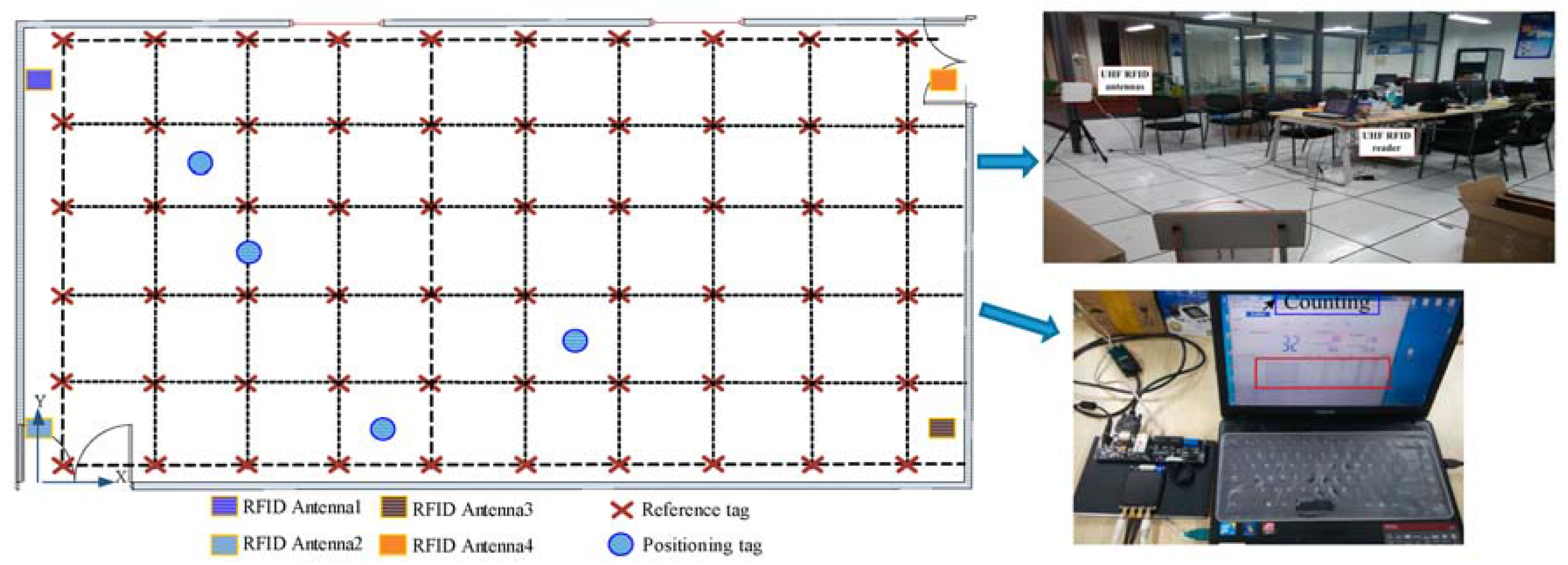
The simulated environment is illustrated as shown in Figure 8. The size of the experimental environment is approximately 11 m × 6 m where a total of 60 reference tags and four UHF RFID antennas were used. The distance between every two adjacent reference tags was 1.2 m, and the four antennas are connected to a reader and fixed in the four different corners of the location area, respectively. When the reader is working, the four antennas will receive the different information (including the RSSI values between the tags and the antennas), which comes from the tag feedback. In order to obtain an accurate RSSI value from the reference tag, the RSSI value of the tag is repeatedly measured 100 times by the antenna at a fixed point, and Gaussian is used to process these RSSI values as described in Section 3.1. Finally, the experiment yielded 240 groups’ perfect sample data elements, including the RSSI values of tags and corresponding positions (60 RSSI data elements for each antenna), and the sample data are regarded as the input values for the ELM network as shown in Figure 9, where
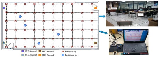
Figure 8.
The simulated experimental environment.
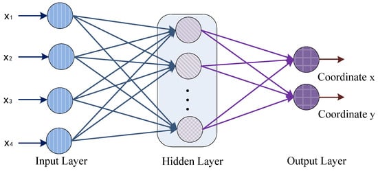
Figure 9.
The architecture of ELM network based on positioning system.
As shown in Figure 9, the architecture of ELM network has nine inputs, each representing a set of RSSI vectors, and two outputs, representing the geography coordinate of the tag position.
4.2. Selection of Parameters for the ELM Model
For the proposed ELM based positioning model, there are two important parameters that need to be selected, namely, the type of activation function and the number of hidden nodes . The sine activation function , hardlim activation function and sigmoid activation function have been used to evaluate the performance of the ELM, with different numbers of hidden nodes. The results of the parameter selection of the optimal number of hidden nodes for ELM with sigmoid, sine and hardlim activation functions are shown in Figure 10.
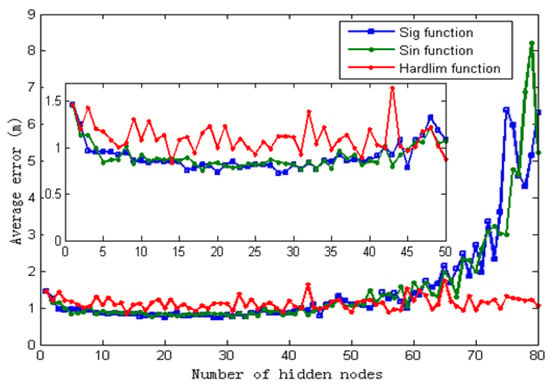
Figure 10.
Average positioning error regarding different activation functions and different numbers of hidden nodes.
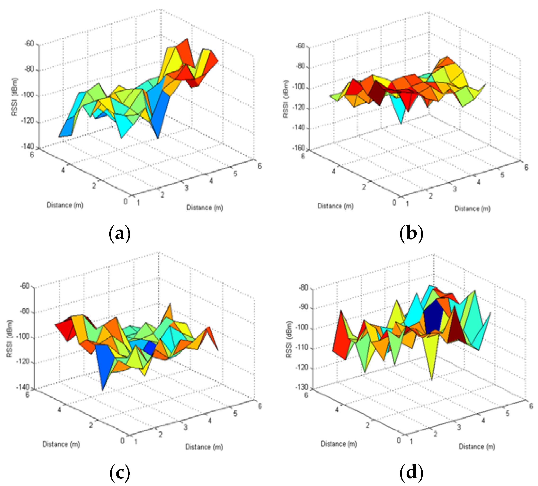
In Figure 10, the performance of ELM with the sigmoid activation function is not significantly changed with respect to the sine activation function. For the sigmoid functions, the increased amplitude of average error is relatively small when the number of hidden nodes was more than 60. In addition, the performance of the hardlim function is the most stable among the three activation functions, but the average error is the worst. Thus, in the following simulations, we selected the sigmoid function as the activation function of ELM, with the number of hidden nodes set to 28, as shown in Table 1. The distribution of RSSI indication from four readers in the experiment is illustrated in Figure 11.

Table 1.
Parameter settings of ELM algorithm.

Figure 11.
The distribution of RSSI indication from four readers: (a) The 3D RSSl values with Reader1; (b) The 3D RSSl values with Reader2; (c) The 3D RSSl values with Reader3; (d) The 3D RSSl values with Reader4.
As shown in Figure 11, the signals collected by one reader can be quite different even at the same location due to noises and RSSI fluctuations in the indoor environment.
4.3. Comparison of Data Quality
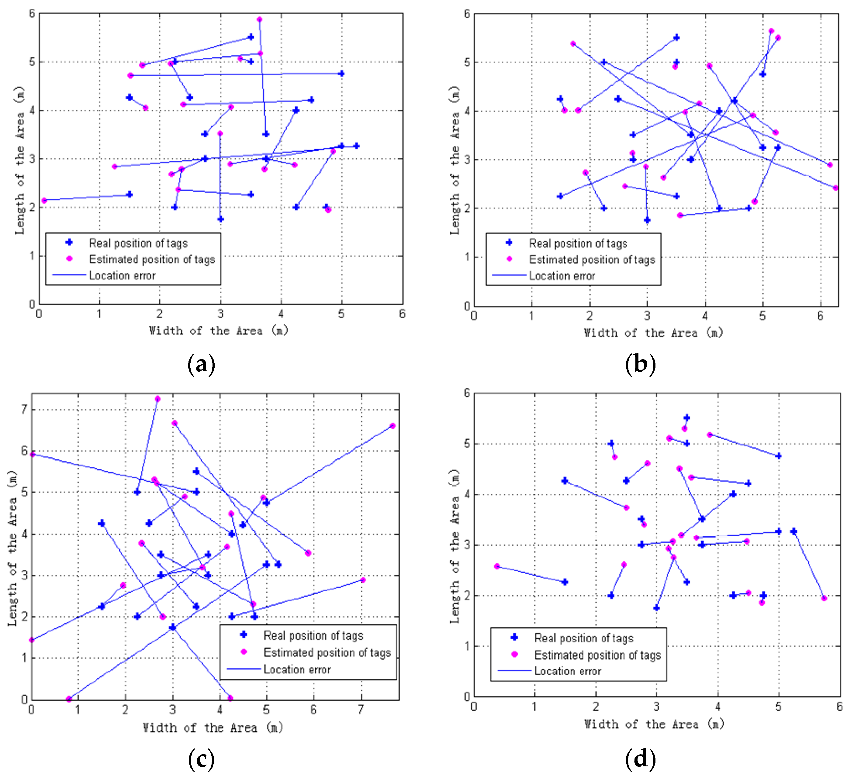
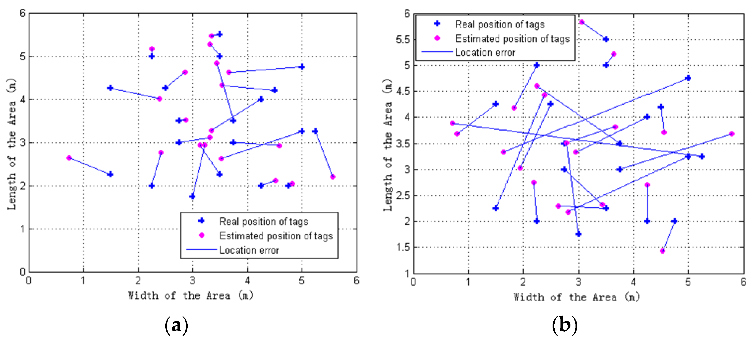
As depicted in Section 3.1, it is seen that the data Gaussian filtering method in the offline and online phases improved the quality of the training data and the model input data, respectively. In order to analyze the influence of the data quality on the precision of the positioning model based on ELM, this study uses the four different scenes, and the algorithm is repeated 10 times in each scenario experiment. The details are as follows and the results of location estimation for impact of data quality on the positioning model is shown in Figure 12. Table 2 summarizes the positioning results in different scenes.
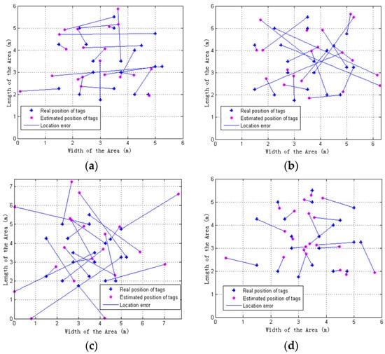
Figure 12.
Impact of data quality on the positioning model: (a) Case 1; (b) Case 2; (c) Case 3; (d) Case 4.

Table 2.
The positioning error results in different scenes (m).
Case 1. In the offline phase, does not filter the training samples; in the online phase, does not filter the test samples for the RSSI information of each tags, and it is used as the input of the model.
Case 2. In the offline phase, does not filter the training samples; however, in the online phase, for the RSSI information of every tag, the reader repeated measurements 100 times at a fixed point, used the Gaussian filter for the collected RSSI, and then used the results as the input of the model.
Case 3. In the offline phase, filtering the training samples according to the corresponding rules in this study; in the online phase, does not filter the test samples for the RSSI information of every tag, and it is used as the input of the model.
Case 4. In the offline phase, filtering the training samples according to the corresponding rules in this study; however, in the online phase, for the RSSI information of every tag, the reader repeated measurements 100 times at a fixed point, used the Gaussian filter for the collected RSSI, and then used the results as the input of the model.
As observed from Table 2, Case 4 has the smallest average error and MSE values—0.7114 and 1.0562, respectively, while Case 3 has the largest average error and MSE values—2.4641 and 3.3730 respectively. Therefore, data filtering in the offline training phase and in the online positioning phase can effectively improve the positioning accuracy of the model. However, we found that, when the positioning model comes from high quality training samples, the input data for online positioning phase also need to be high quality.
4.4. Comparison with Other Algorithms
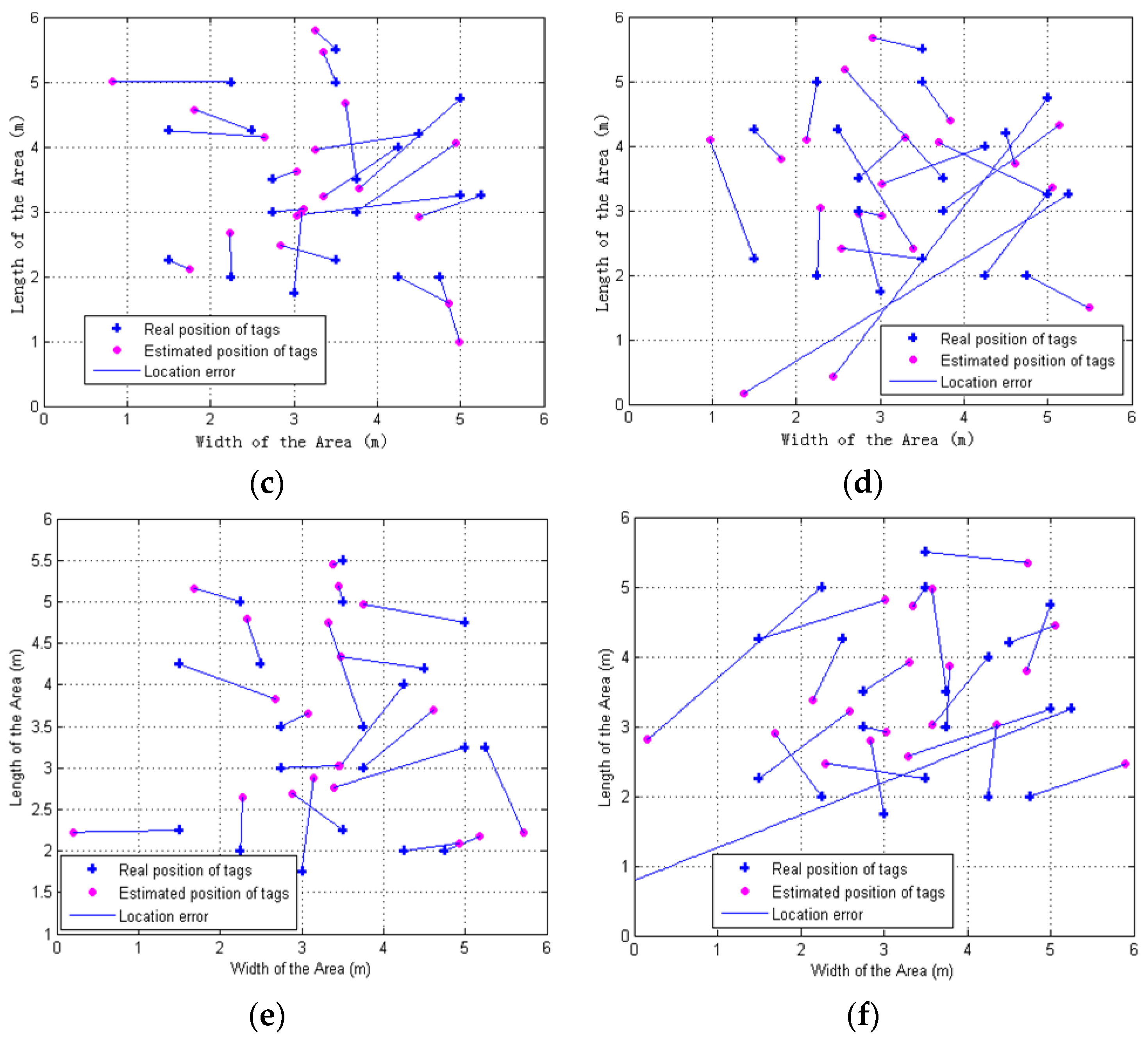
This section aims to further evaluate the performance of the proposed algorithm. The GA-BP, PSO-BP positioning method [30,31] with no filtering training and testing samples are implemented and compared, respectively, and the evaluation criteria include the positioning error and algorithm running time. Since the same ANN structure and the same training set might draw a different result, each positioning algorithm run 10 times repeatedly. The results of location estimation for different positioning methods are presented in Figure 12, and the positioning error results are summarized in Table 3.

Table 3.
The positioning error results for different positioning methods (m).
4.4.1. Positioning Error
It can be seen from Figure 13 and Table 3 that the positioning accuracy of the proposed ELM-Gaussian filtering method is obviously superior to other five methods such as ELM (without Gaussian filtering), GA-BP-Gaussian filtering (include filtering training and testing samples) and GA-BP (without Gaussian filtering), PSO-BP-Gaussian filtering (include filtering training and testing samples) and PSO-BP (without Gaussian filtering). ELM-Gaussian filtering enhances the average positioning error by 47.05% over ELM, 22.18% over GA-BP-Gaussian filtering, 47.47% over GA-BP, 12.68% over PSO-BP-Gaussian filtering, 55.69% over PSO-BP, GA-BP-Gaussian filtering enhances the average positioning error by 32.50% over GA-BP, and PSO-BP-Gaussian filtering enhances the average positioning error by 49.26% over PSO-BP. However, the ELM (without Gaussian filtering) and the GA-BP (without Gaussian filtering) provide similar average positioning error, which is 1.3237 m and 1.3343 m, respectively.
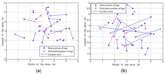
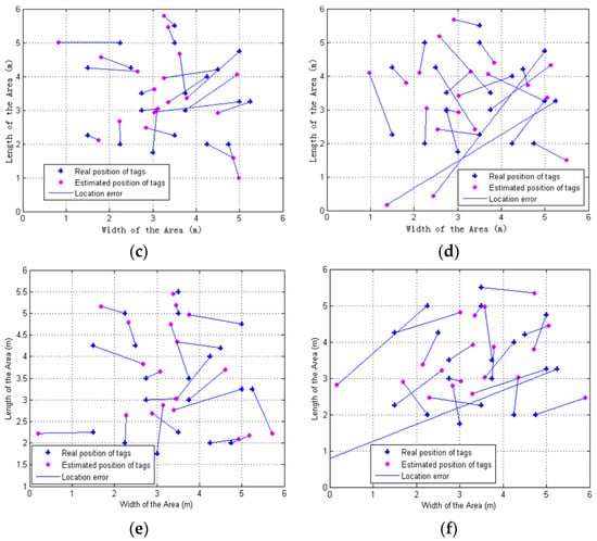
Figure 13.
Comparison with the other positioning methods: (a) ELM-Gauss filtering (include filtering training and testing samples); (b) ELM (without Gauss filtering); (c) GA-BP-Gaussian filtering (include filtering training and testing samples); (d) GA-BP (without Gaussian filtering); (e) GA-BP-Gaussian filtering (include filtering training and testing samples); (f) GA-BP (without Gaussian filtering).
Therefore, effective data filtering (including filtering training and test samples) can greatly improve the positioning accuracy based on machine learning methods, and the average positioning accuracy of the ELM method is better than the GA-BP and PSO-BP method.
4.4.2. Computational Time
In order to further evaluate the performance of the proposed algorithm, the efficiency of three machine learning algorithms (ELM, GA-BP and PSO-BP) based on positioning was compared, and each positioning algorithm ran three times continuously. Table 4 and Table 5 list the parameters of GA-BP and PSO-BP algorithms based on positioning, respectively, and Table 6 lists the computational time for three algorithms. In terms of computational time, as observed from Table 6, ELM requires at most 0.5156 s in the training phase, reducing the training time over GA-BP (4.2998 s) by a factor of 8, and reducing the training time over PSO-BP (3.9891 s) by a factor of 7, and ELM requires at most 0.1078 s in the testing phase, reducing the testing time over GA-BP (1.5326 s) by a factor of 1, and reducing the testing time over PSO-BP (1.5198) by a factor of 2. This demonstrates that the ELM algorithm is superior to the GA-BP and PSO-BP learning algorithms in the RFID-enabled positioning systems, since the core of ELM is to transform the complex iterative process into the random generation of hidden layer parameters.

Table 4.
Parameter setting of GA-BP algorithm.

Table 5.
Parameter setting of PSO-BP algorithm.

Table 6.
The performance comparison of training and testing time.
5. Discussion
Based on the obtained results, it can be concluded that the ELM regression model could achieve a higher computational efficiency in the positioning system, since it only needs to set up the hidden nodes number, and the algorithm does not need to adjust the input weights and the bias of the network. Additionally, indoor positioning based on RFID will display the phenomenon of signal reflection and fading due to the space layout and multipath effects in indoor environment, which will lead to the larger fluctuations of signal strength in the acquired data samples. Therefore, the Gaussian filtering is proposed to reduce the signal fluctuation of RSSI, and our experiments verify that ELM-Gaussian filtering (including filtering training and testing samples) can provide high positioning accuracy compared with the other five methods. We conclude that the combination of Gaussian filtering (include filtering training and testing samples) and ELM can effectively solve the positioning problem in the indoor environments.
6. Conclusions
The data qualities of the online and offline phases are analyzed, respectively, which shows that the high quality positioning model can obviously improve the accuracy of indoor positioning. In addition, the time consumption of indoor positioning is also analyzed and compared, and the proposed algorithm estimates the current coordinate of the tag by building the ELM positioning model combined with the RSSI measurement values and achieves a rapid positioning.
In this study, to solve the inaccurate localization and efficiency problems in a complex positioning system, an ELM algorithm based on Gaussian filtering is proposed, which introduces the Gaussian filtering rule and can effectively filter out the significant fluctuant signals that are caused by the environment effects, and provide a high quality sample data. The proposed ELM-Gaussian filtering methods can quickly establish a high quality positioning model and achieve a fast position prediction. The experimental results demonstrate that the proposed positioning system will contribute by effectively avoiding the environment interferences and achieving the highest accuracy and efficiency in all comparative methods.
Future research directions will be concerned with the following issues. Firstly, different scenarios can be implemented for testing the robustness of the proposed algorithm. Secondly, other wireless communication network-based localization methods will be tested for their feasibilities in the complex and dynamic experimental environment.
Acknowledgments
Support of our work by the National Natural Science Foundation of China (No. 61272097), the Shanghai Municipal Committee of Science and Technology Project (No. 13510501400), the Innovation Program Alliance of Shanghai University of Engineering Science (No. E1-0702-15-01032-2013lm01), the Natural Science Foundation of Shanghai (17ZR1411900), the Opening Project of Shanghai Key Laboratory of Integrated Administration Technologies for Information Security (AGK2015006), the Founding Program for the Cultivation of Young University Teachers of Shanghai (ZZGCD 15090), and the Research Start-up Founding Program of Shanghai University of Engineering Science (2016-56) is gratefully acknowledged.
Author Contributions
Changzhi Wang constructed the model and the algorithm and wrote the manuscript; Zhicai Shi and Fei Wu provide the instructions and helps during the design. All authors provide the helps in revisions of this manuscript. All authors have read and approved the final manuscript.
Conflicts of Interest
The authorsdeclare no conflict of interest.
References
- Akyildiz, I.F.; Su, W.L.; Sankarasubramaniam, Y.; Cayirci, E. A survey on sensor networks. IEEE Commun. Mag. 2002, 40, 102–114. [Google Scholar] [CrossRef]
- Gressmann, B.; Klimek, H.; Turau, V. Towards Ubiquitous Indoor Location Based Services and Indoor Navigation. In Proceedings of the 2010 7th Workshop on Positioning Navigation and Communication (WPNC), Dresden, Germany, 11–12 March 2010; pp. 107–112.
- Lee, D.; Chung, W. Discrete-status-based localization for indoor service robots. IEEE Trans. Ind. Electron. 2006, 53, 1737–1746. [Google Scholar] [CrossRef]
- Moghtadaiee, V.; Dempstera, A.G. Indoor location fingerprinting using FM radio signals. IEEE Trans. Broadcast. 2014, 60, 336–346. [Google Scholar] [CrossRef]
- Luo, X.W.; O’Brien, W.J.; Julien, C.L. Comparative evaluation of received signal-strength index (RSSI) based indoor localization techniques for construction jobsites. Adv. Eng. Inform. 2011, 25, 355–363. [Google Scholar] [CrossRef]
- Benavente-Peces, C.; Moracho-Oliva, V.M.; Dominguez-Garcia, A.; Lugilde-Rodriguez, M. Global system for location and guidance of disabled people: indoor and outdoor technologies integration. In The Fifth International Conference on Networking and Services; IEEE Press: Valencia, Spain, 2009; pp. 370–375. [Google Scholar]
- Shiraishi, T.; Komuro, N.; Ueda, H.; Kasai, H.; Tsuboi, T. Indoor Location Estimation Technique using UHF band RFID. In Proceedings of the International Conference on Information Networking, Busan, Korea, 23–25 January 2008; pp. 1–5.
- Wang, C.S.; Chen, C.C. Flexible localization and identification system based on RFID and vision tracking technologies. In Proceedings of the 2011 International Symposium on Computer Science and Society, Kota Kinabalu, Malaysia, 16–17 July 2011; pp. 356–360.
- Montaser, A.; Moselhi, O. RFID indoor location identification for construction projects. Autom. Constr. 2014, 39, 167–179. [Google Scholar] [CrossRef]
- Goodrum, P.M.; McLaren, M.A.; Durfee, A. The application of active radio frequency identification technology for tool tracking on construction job sites. Autom. Constr. 2006, 15, 292–302. [Google Scholar] [CrossRef]
- Yang, Z.X.; Zhang, P.B.; Chen, L. RFID-enabled indoor positioning method for a real-time manufacturing execution system using OS-ELM. Neurocomputing 2016, 174, 121–133. [Google Scholar] [CrossRef]
- Wu, Z.; Jedari, E.; Muscedere, R.; Rashidzadeh, R. Improved particle filter based on WLAN RSSI fingerprinting and smart sensors for indoor localization. Commput. Commun. 2016, 83, 64–71. [Google Scholar] [CrossRef]
- Wu, H.; Chang, Y.; Hwang, M.; Lin, I. Flexible RFID location system based on artificial neural networks for medical care facilities. SIGBED Rev. 2009, 6, 12. [Google Scholar] [CrossRef]
- Kuo, R.J.; Shieh, M.C.; Zhang, J.W.; Chen, K.Y. The application of an artificial immune system-based back-propagation neural network with feature selection to an RFID positioning system. Robot. Comput. Integr. Manuf. 2013, 29, 431–438. [Google Scholar] [CrossRef]
- Ceravolo, F.; Felice, M.D.; Pizzuti, S. Combining back-propagation and genetic algorithms to train neural networks for ambient temperature modeling in Italy. Lect. Notes Comput. Sci. 2009, 5484, 123–131. [Google Scholar]
- Zou, H.; Wang, H.; Xie, L.; Jia, Q.-S. An RFID indoor positioning system by using weighted path loss and extreme learning machine. In Proceedings of the 2013 IEEE 1st International Conference on Cyber-Physical Systems, Networks, and Applications (CPSNA), Taipei, Taiwan, 19–20 August 2013; pp. 66–71.
- Jiang, X.L.; Chen, Y.Q.; Liu, J.F.; Liu, D.J.; Gu, Y.; Chen, Z.Y. Real-time and accurate indoor localization with fusion model of wi-fi fingerprint and motion particle filter. Math. Probl. Eng. 2015, 2015, 545792. [Google Scholar] [CrossRef]
- Fu, H.; Vong, C.M.; Wong, P.K.; Yang, Z. Fast detection of impact location using kernel extreme learning machine. Neural Comput. Appl. 2016, 27, 121–130. [Google Scholar] [CrossRef]
- Lee, C.W.; Lin, T.N.; Fang, S.H.; Chou, Y.H.; Chou, Y.C. A novel clustering-based approach of indoor location fingerprinting. In Proceedings of the 2013 IEEE 24th International Symposium on Personal, Indoor and Mobile Radio Communications (PIMRC Workshops), London, UK, 8–9 September 2013; pp. 3191–3196.
- Lin, T.N.; Fang, S.H.; Tseng, W.H.; Lee, C.W.; Hsieh, J.W. A group-discrimination-based access point selection for WLAN fingerprinting localization. IEEE Trans. Veh. Technol. 2014, 63, 3967–3976. [Google Scholar] [CrossRef]
- Kegen, Y.; Jay, G.Y. Statistical NLOS identification based on AOA, TOA and signal strength. IEEE Trans. Veh. Technol. 2009, 58, 274–286. [Google Scholar]
- Yassin, M.; Rachid, E.; Nasrallah, R. Performance Comparison of Positioning Techniques in Wi-Fi Networks. In Proceedings of the 2014 10th International Conference on Innovations in Information Technology (INNOVATIONS), Al-Ain, UAE, 9–11 November 2014; pp. 75–79.
- Hatami, A.; Alavi, B.; Pahlavan, K.; Kanaan, M. A Comparative Performance Evaluation of Indoor Geolocation Technologies. Interdiscip. Inf. Sci. 2006, 12, 133–146. [Google Scholar] [CrossRef]
- Choi, J.S. Accurate and Cost Efficient Object Localization Using Passive UHF RFID. Ph.D. Thesis, University of Texas at Arlington, Arlington, TX, USA, 2011. [Google Scholar]
- Huang, G.B.; Zhu, Q.Y.; Siew, C.K. Extreme learning machine: A new learning scheme of feedforward neural networks. In Proceedings of the IEEE International Joint Conference on Neural Networks, Budapest, Hungary, 25–29 July 2004; Volume 2, pp. 985–990.
- Huang, G.B.; Chen, L.; Siew, C.K. Universal approximation using incremental constructive feedforward networks with random hidden nodes. IEEE Trans. Neural Netw. 2006, 17, 879–892. [Google Scholar] [CrossRef] [PubMed]
- Li, M.B.; Huang, G.B.; Saratchandran, P.; Sundararajan, N. Fully complex extreme learning machine. Neurocomputing 2005, 68, 306–314. [Google Scholar] [CrossRef]
- Huang, G.; Song, S.; Gupta, J.N.; Wu, C. Semi-supervised and unsupervised extreme learning machines. IEEE Trans. Cybern. 2014, 44, 2405–2417. [Google Scholar]
- Huang, G.B.; Zhu, Q.Y.; Siew, C.-K. Extreme learning machine: Theory and applications. Neurocomputing 2006, 70, 489–501. [Google Scholar] [CrossRef]
- Tran, D.A.; Nguyen, T. Localization in wireless sensor networks based on support vector machines. IEEE Trans. Parallel Distrib. Syst. 2008, 19, 981–994. [Google Scholar] [CrossRef]
- Yang, G.; Chen, C.; Jian, Y. An Indoor Localization Algorithm Based on RBF Neural Network Optimized by the Improved PSO. In Proceedings of the International Conference on Electronic, Information Technology and Intellectualization (ICEITI), Guangzhou, China, 11–12 June 2016; pp. 457–464.
© 2017 by the authors. Licensee MDPI, Basel, Switzerland. This article is an open access article distributed under the terms and conditions of the Creative Commons Attribution (CC BY) license ( http://creativecommons.org/licenses/by/4.0/).

