BSLIC: SLIC Superpixels Based on Boundary Term

Abstract

A modified method for better superpixel generation based on simple linear iterative clustering (SLIC) is presented and named BSLIC in this paper. By initializing cluster centers in hexagon distribution and performing k-means clustering in a limited region, the generated superpixels are shaped into regular and compact hexagons. The additional cluster centers are initialized as edge pixels to improve boundary adherence, which is further promoted by incorporating the boundary term into the distance calculation of the k-means clustering. Berkeley Segmentation Dataset BSDS500 is used to qualitatively and quantitatively evaluate the proposed BSLIC method. Experimental results show that BSLIC achieves an excellent compromise between boundary adherence and regularity of size and shape. In comparison with SLIC, the boundary adherence of BSLIC is increased by at most 12.43% for boundary recall and 3.51% for under segmentation error.

1. Introduction

Although superpixels were firstly described as over-segmentations by Ren and Malik in 2003, they have still not been exactly defined [1,2]. Generally, a superpixel can be treated as the set of pixels that are similar in location, color, texture, etc. Superpixels can capture image redundancy and transform pixel-level computing into a region-level operation [3], which can greatly reduce the complexity of subsequent image processing tasks. Superpixel segmentation has become an important pre-processing step in various image processing applications, such as image segmentation [4,5,6,7,8,9], saliency detection [10,11,12] and classification [13,14].

Existing superpixel segmentation methods can be classified into three major categories: the spectral-graph-based method, the gradient-ascent-based method and the optimization-theory-based method. The spectral-graph-based method is an optimal procedure to globally minimize the graph-based objective functions [15]. This method treats image pixels as the nodes of graph and sets the edge weights of the graph proportional to the affinities between neighboring pixels [3]. Shi and Malik proposed the Normalized Cut (NCut) criterion for graph segmenting [16]. Although NCut generates superpixels of a similar size and compact shapes [3], its complexity brings a heavy burden into the computation works. Felzenszwalb and Huttenlocher (FH) [17] is another typical spectral-graph-based algorithm, which has a complexity of $O\left(NlogN\right)$ [18] and is faster than NCut. However, the superpixels generated by FH are very irregular in size and shape. The gradient-ascent-based method forms superpixels by updating the clustering of pixels in the direction of gradient ascent until a certain convergence criterion is met [3]. Mean Shift (MS) [19] and Quick Shift (QS) [20] are two gradient-ascent-based methods. They have complexities of $O\left(N^2\right)$ and $O\left(d{N}^2\right)$ ($d$ is a small constant) respectively, and the superpixels generated by them are still irregular in shape [3]. Turbopixel [21] is another gradient-ascent-based algorithm, which can provide more regular superpixels and shorten the processing time to $O\left(N\right)$ [3]. The optimization-theory-based method formulates the image segmentation as a minimization problem of energy function, which is derived from image information. SuperPB [22] and SEEDS [15] are two classical methods based on optimization theories. SuperPB generates superpixels by minimizing two pseudo-boolean functions, and its computing speed is independent from the superpixels number. SEEDS is a two-stage method, which firstly segments the image into coarse superpixels and then refines the boundaries. The energy function of SEEDS is established based on the color similarity and histogram of the initial superpixels. Thus, SEEDS features an excellent compromise between accuracy and efficiency.

SLIC (Simple Linear Iterative Clustering) is the most widely used superpixel method. Essentially, it is a local k-means clustering method [3], and does not belong to the above three categories. SLIC groups pixels into perceptually meaningful regions in a five-dimensional feature space, which is defined by the CIELAB color space and the $x, y$ pixel coordinates. Compared with the above-mentioned methods, SLIC has several advantages. Firstly, SLIC has lower complexity. For $N$ image pixels, the complexity of SLIC is just $O\left(N\right)$. Secondly, SLIC can generate superpixels with compact, regular size and shape. Moreover, SLIC is simple to use and understand [3,23].

Figure 1 displays the segmentation results of SEEDS, SuperPB, SLIC and Turbopixel. Numbers of the generated superpixels are the same or approximate. The edges that cannot be extracted by superpixels are labelled with a white dotted line. It can be observed from the first row that SEEDS possesses the worst regularity in size and shape. Turbopixel is much better than SEEDS, but still worse than SuperPB and SLIC. The second row is the partial enlarged images for the region containing image edges. It is observed that SEEDS owns higher boundary adherence, while the other three methods cluster more pixels of slender rod and sky into one superpixel. Segmentation results suggest that SLIC provides a relatively better compromise between boundary adherence and regularity. However, the boundary adherence of the superpixels generated by it still needs to be improved.

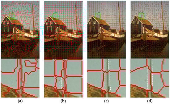
Figure 1. Superpixel segmentation results of four algorithms. (a) SEEDS; (b) SuperPB; (c) simple linear iterative clustering (SLIC); (d) Turbopixels. The second row is the partial enlarged superpixels defined by the green rectangles.

In this paper, based on SLIC, an improved superpixel method is proposed to achieve an excellent compromise between boundary adherence and the regularity of size and shape. Boundaries and regions are two affinitive cues for humans to perform segmentation [24]. As the small regions in an image domain, superpixels rely on region information more than boundary information. In order to efficiently align the SLIC superpixels to image edges and obtain better segmentation results, a global usage of boundary and region information is conducted. In contrast to the previous method, which utilizes multi-scale boundary information to segment a specific image region instead of the whole scene [25], this paper adopts a simple edge detecting algorithm to obtain the complete boundary information. Herein, the modified SLIC is expressed as BSLIC, where B stands for the boundary term. The advantages of BSLIC are summarized as follows: First, the modified method features competitive boundary adherence, which can be validated by qualitative and quantitative experiments on databases BSDS500 [26]. Second, BSLIC, which only modifies two steps of SLIC, is very simple to use and understand. Third, the superpixels generated by BSLIC have good compactness and regularity in size and shape, which is an effective inheritance from SLIC.

The rest of the paper is organized as follows: Section 2 provides an overview of the algorithm. Section 3 introduces the proposed BSLIC algorithm, including the distribution of cluster centers, the initialization of edge centers and the distance measurement. Section 4 shows the experimental results and necessary discussions. Finally, Section 5 concludes the paper.

2. Overview of BSIC

BSLIC is essentially a k-means clustering method. The data points of BSLIC are vectors that describe the features of image pixels. In fact, spectral clustering [27] and subspace clustering [28] are also capable of implementing the clustering of image pixels. However, the memory of these two kinds of methods are demanding. Both the spectral clustering and the subspace clustering method have to compute the affinity matrix of data points, which is an $n\times n$ matrix for an image with $n$ pixels. For images with moderate resolution, such as $321\times 481$, the affinity matrix would take up more than $2\times {10}^{10}$ memory cells. As a pre-processing step, superpixels should be fast to compute, memory-efficient and simple to use. So, in our BSLIC, the k-means method is chosen to implement the clustering of image pixels.

Figure 2 illustrates the flow chart of BSLIC. In BSLIC, two kinds of cluster centers, “plane center” and “edge center” are initialized. We first initialize plane centers (red dots) in a hexagon distribution. For each plane center, an edge pixel within its local searching region is initialized as an edge center, and these are marked by green dots. A canny operator, the most widely used edge detecting algorithm, is utilized to obtain the boundary information, and the boundary term is then incorporated into the local k-means clustering. For each iteration, the pixel-wise distance is dependent on the boundary term. If there exists an edge pixel along the straight line connecting the two pixels, the distance is set as Inf; otherwise, it is calculated as the weighted sum of color and space Euclidean distance. The iterating process is terminated when the residual error is less than 5%, and the iterating time is often no more than 10 [2].

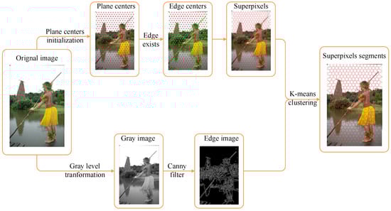
Figure 2. The flow chart of the proposed BSLIC algorithm.

3. Algorithm of BSLIC

The SLIC algorithm has been described by [3] in detail. In this section, only the differences between BSLIC and SLIC are presented. The BSLIC algorithm is different from SLIC in the following three aspects: initializing cluster centers in hexagon rather than square distribution, additionally choosing some specific edge pixels as cluster centers, incorporating boundary term into the distance measurement during k-means clustering. The technical details are discussed below.

3.1. Distribution of Cluster Centers

In SLIC, the initialized cluster centers are squarely distributed as shown in Figure 3a. Centers $C_{i0}$, $C_{i1}$, $C_{i2}$, $C_{i3}$, $C_{i4}$, $C_{i5}$, $C_{i6}$, $C_{i7}$ and $C_{i8}$ are sampled with an interval of $S_0$ pixels. Rectangles in a black solid line are initialized superpixels. Given the number of image pixels $N$ and the desired superpixels number $k$, the interval $S_0$ can be obtained as:

$$S_0=\sqrt{\frac{N}{k}}$$

(1)

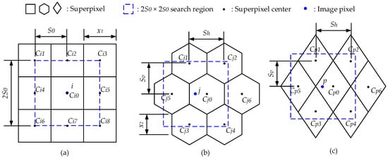
Figure 3. Distribution of Cluster Centers. (a) Square distribution; (b) Hexagon distribution; (c) Diamond distribution.

Square superpixels display central symmetry, but the regions containing the image edges are generally asymmetric. In order to improve the boundary adherence of superpixels across image edges, the symmetry properties of superpixels are reduced from central symmetry to axial symmetry. Both hexagons and diamonds display axial symmetry. Below, the initializing centers in hexagon and diamond distributions are discussed.

Figure 3b displays the geometric sketch of a hexagon distribution. Centers $C_{j0}$, $C_{j1}$, $C_{j2}$, $C_{j3}$, $C_{j4}$, $C_{j5}$ and $C_{j6}$ are sampled at intervals of $S_h$ pixels in the horizontal direction, and $S_v$ pixels in the vertical direction. Hexagons in the black solid line are superpixels. To make the hexagon superpixel equal to the square superpixel in area, side lengths of the square and hexagon should follow the mathematical relationship:

$$\frac{x_1^2}{x_2^2}=\frac{3\sqrt{3}}{2}$$

(2)

where $x_1$ and $x_2$ are the side lengths of the square and hexagon, and $x_1$ is obtained by:

$$x_1=\sqrt{\frac{N}{k}}$$

(3)

For a hexagon distribution, the horizontal and vertical intervals are given as:

$$S_h=\sqrt{3}{x}_2$$

(4)

$$S_v=\frac{3}{2}{x}_2$$

(5)

Combining Equations (2)–(5), $S_h$ and $S_v$ are obtained as:

$$S_h=\sqrt{\frac{N}{\left(\raisebox{1ex}{$\sqrt{3}$}\!\left/ \!\raisebox{-1ex}{$2$}\right.\right)·k}}$$

(6)

$$S_v=\sqrt{\frac{\sqrt{3}}{2}·\frac{N}{k}}$$

(7)

For diamond distribution, which is displayed in Figure 3c, its horizontal and vertical intervals are equal to that of the hexagon distribution.

SLIC performs k-means clustering within the $2S_0\times 2S_0$ local region of pixels. For a square distribution, there are at most nine adjacent superpixels within the local region. Pixel $i$ in Figure 3a depicts this. The $2S_0\times 2S_0$ local searching region of $i$ is marked by the rectangle in the blue dotted line, there exist nine adjacent superpixels ($C_{i0}$, $C_{i1}$, $C_{i2}$, $C_{i3}$, $C_{i4}$, $C_{i5}$, $C_{i6}$, $C_{i7}$ and $C_{i8}$) in the scope. This means that, at most, nine distance calculations are needed for the assignment of one pixel. The complexity for each iteration of the clustering is 9$N$. Compared with square distribution, the hexagon distribution has a lower complexity of 6$N$ for one iteration of the clustering. As shown in Figure 3b, there are six adjacent superpixels ($C_{j0}$, $C_{j1}$, $C_{j2}$, $C_{j3}$, $C_{j4}$ and $C_{j5}$) in the local searching scope of pixel $j$. The complexity of the diamond distribution is also 6$N$, which is displayed in Figure 3c.

Performing k-means clustering in a limited size, rather than the whole image domain, is the key point to speed up the SLIC algorithm because it largely reduces the number of distance calculations. By initializing cluster centers in the hexagon or diamond distribution, the number of distance calculations can decrease by 3$N$. With the same sample intervals, cluster centers initialized in the hexagon distribution are the same as that of the diamond distribution. In other words, the superpixel segmentation results of the hexagon distribution are the same as that of the diamond distribution. In our work, cluster centers are initialized in the hexagon distribution.

3.2. Initialization of Edge Centers

The superpixels across the ground truth edges, which are called the edge-across superpixels, are the root cause of under segmenting. Edge-across superpixels are displayed in Figure 4c,d. Their cluster centers are initialized in the hexagon and square distribution respectively. The white and red solid lines describe the image edges and the superpixels’ boundaries. Each closed region in a red solid line represents a superpixel. The edge-across superpixels are denoted as ${\mathrm{F}}_i$, and the accurate superpixels are denoted as ${\mathrm{R}}_i$, which refers to the superpixels that exactly align to the ground truth edges. The subscript $i$ plays the role of counting the superpixels. It is found that the edge-across and accurate superpixels have a similar size. As shown in Figure 4c, the edge-across superpixels ${\mathrm{F}}_1$ and ${\mathrm{F}}_2$ have 67 and 101 pixels, while the accurate superpixels ${\mathrm{R}}_1$, ${\mathrm{R}}_2$ and ${\mathrm{R}}_3$ have 99, 122 and 126 pixels. For images with a resolution of $481\times 321$, regions in $8\times 8$ size (approximately 67 pixels) are hardly different from regions in $11\times 11$ (approximately 126 pixels). In order to improve the boundary adherence of edge-across superpixels, the area of edge-across superpixels should be decreased.

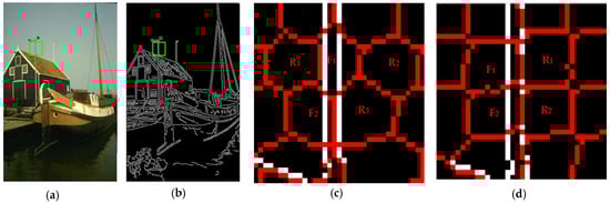
Figure 4. Edge-across superpixels. (a) Original image with slender rod; (b) Edge image with canny filter operator; (c) Partial enlarged superpixels with only plane centers initialized in hexagon distribution; (d) Partial enlarged superpixels with only plane centers initialized in square distribution.

Edge-across superpixels are the small regions containing image edges, while the edges are the place where discontinuity in intensity or color happens. For an edge-across superpixel, pixels located in two sides of the edge are very dissimilar. To assign these pixels two superpixels, the exact edge pixels are chosen as cluster centers. Centers initialized from edge pixels are called “edge center”, and those that are initialized in a uniform geometric distribution are called “plane center”. The two kinds of cluster centers are illustrated in Figure 5. Edge center is determined by the following rules:

• If there exist image edges in the $S_0\times S_0$ searching region of plane center (like $C_{i1}$), choose a median edge pixel as the edge center (like $E_{i1}$);
• If there is no image edge within the $S_0\times S_0$ region (like $C_{i4}$), no edge center is generated;
• To avoid any noisy pixel being chosen as cluster center, modify the edge center to the lowest gradient position in the corresponding $3\times 3$ local neighborhood;
• Edge center is introduced to reduce the negativity of edge-across superpixels. It is necessary to keep it near to the image edges. During the 10 iterations, edge centers remain unalterable, and only plane centers are updated to the mean value.

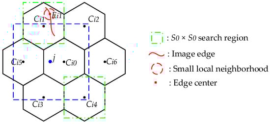
Figure 5. Plane center and edge center. Dots in solid black $C_{i0}$, $C_{i1}$, $C_{i2}$, $C_{i3}$, $C_{i4}$, $C_{i5}$ and $C_{i6}$ are “plane center”; Square in solid red $E_{i1}$ is “edge center”.

Superpixel segmentation results with initialized edge centers are displayed in Figure 6. Compared with Figure 4c, the edge-across superpixel ${\mathrm{F}}_1$ is successfully transformed into the accurate superpixel ${\mathrm{R}}_4$ in Figure 6a, which can improve boundary adherence to some degree. However, when it comes to square distribution, there is no apparent decrease in area for edge-across superpixels ${\mathrm{F}}_1$ and ${\mathrm{F}}_2$, as shown in Figure 4d and Figure 6b.

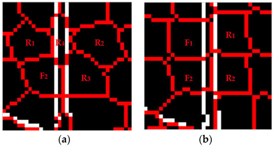
Figure 6. Partial enlarged superpixels segmentation with edge cluster centers initialized. (a) Plane centers initialized in a hexagon distribution; (b) Plane centers initialized in a square distribution.

We owe the better segmentation results of Figure 6a to the asymmetry of the edge-across superpixel. For small regions without image details, such as edges and texture, the pixels possess high similarity with others. These small regions can be described as possessing local symmetry to some degree. However, this is inconsistent for edge-across superpixels, the pixels of which are located on two sides of the edge and are very dissimilar. Edge-across superpixels are asymmetrical in the local region. Compared with superpixels initialized in square distribution, the hexagon distribution reduces the central and axial symmetry. Moreover, initializing edge centers largely destructs the horizontal and vertical symmetry of the initialized superpixels.

3.3. Distance Measurement

From Figure 4c to Figure 6a, there is no apparent decrease in the area of edge-across superpixel ${\mathrm{F}}_2$. This part introduces an available method to reduce the area of ${\mathrm{F}}_2$. In SLIC, the distance between pixels is defined as the weighted sum of color and spatial Euclidean distance. For the pixels that are similar in spatial locations and color but belong to different objects, such as pixels $i$ and $j$ shown in Figure 7a, SLIC tends to assign them to one superpixel. Setting a large value for the distance between $j$ and $C_i$ is an effective way to assign $i$ and $j$ to different superpixels.

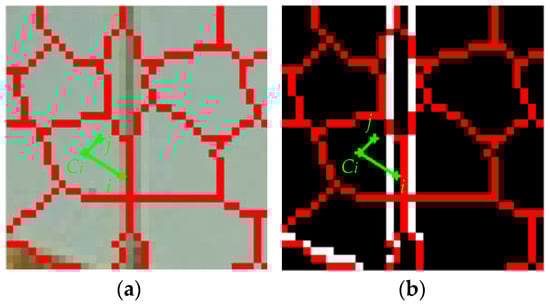
Figure 7. Boundary term incorporation. (a) Partial enlarged superpixels on original image; (b) Partial enlarged superpixels on logical edge image.

Herein, the given pair of pixels is connected by straight line over the image domain. The boundary term is incorporated by checking the presence of image edge along the straight line. Figure 7 illustrates this process. The edge image, which is obtained by a canny operator, is a binary image. In fact, any existing edge detecting algorithms, such as Sobel, Robert, etc., are suitable for the work. Our problem is transformed into checking if there exists a nonzero element along the straight line. If it exists, such as pixel $i$ and center $C_i$ shown below, the distance would be Inf. Otherwise, like $j$ and $C_i$, the distance would be calculated as the weighted sum of color and spatial Euclidean distance. The modified distance equation can be described as follows:

$$d=\{\begin{array}{c}\sqrt{d_c^2+m^2·{\left(\frac{d_s}{S_0}\right)}^2},Noedge\\ Inf,Edgeexits\end{array}$$

(8)

where $d_c$ and $d_s$ are color and spatial Euclidean distances. Parameter $m$ is the weighting factor. It is suggested that $m$ should be in the range of [1, 40] in CIELAB color space [3].

Superpixel segmentation results are shown in Figure 8 with boundary term incorporated. Compared with Figure 6a, our distance measurement successfully transforms the edge-across superpixel ${\mathrm{F}}_2$ into accurate superpixel ${\mathrm{R}}_5$, realizing a further progress in improving boundary adherence.

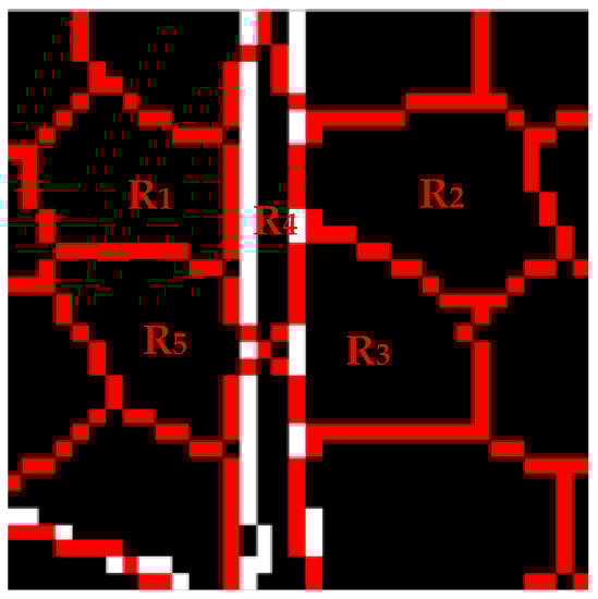
Figure 8. Superpixels segmentation result with modified distance calculation.

4. Experimental Results

In this section, we first discuss some important issues of BSLIC, including the iterating process and the effects of parameters. Then the evaluation of the BSLIC is presented together with other four algorithms. Qualitative and quantitative experimental results are all displayed, and necessary comparison is carried out to validate the competitive performance of BSLIC.

4.1. BSLIC Superpixels

The iterating process of BSLIC is displayed in Figure 9. Figure 9a shows the superpixels with only plane centers initialized, in which the superpixels have good axial symmetry in both the horizontal and vertical directions. Figure 9b is the superpixels with edge centers initialized. It is obvious that the axial symmetry of the edge-cross superpixels is destroyed. Figure 9c,d are the first and final iterating results. Compared to the final results, the first iteration has already aligned to the true boundaries in the whole picture.

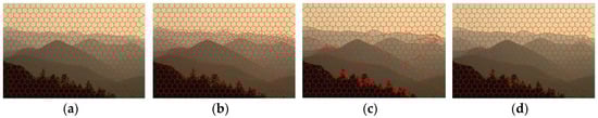
Figure 9. BSLIC iterating process. (a) Superpixels with only plane centers; (b) Superpixels with both plane and edge centers; (c) First iterating result of BSLIC; (d) Final segmentation result of BSLIC.

The $L_2$ norm is adopted to compute the residual error between two iterations. In BSLIC, the iteration of k-means clustering is not terminated until the residual error of the cluster centers is less than 5%. In the simulation experiments, we found that small changes of superpixel segmentation results happened after five or six iterations. Figure 10 displays the change curve of residual error against iterating times. After 10 or fewer times, the residual error becomes convergent, which is consistent with the empirical data in [3].

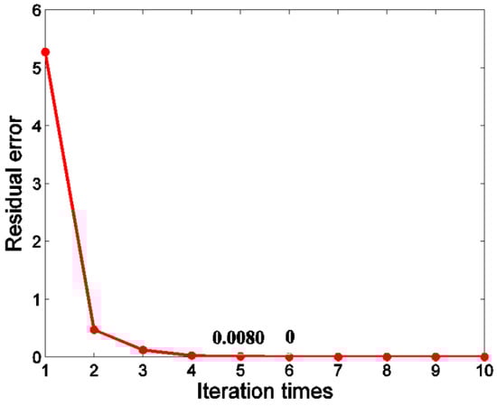
Figure 10. Change curve of residual error against iterating times.

Figure 11 shows the BSLIC segmentation results with different $k$ and $m$. It is indicated that larger $m$ achieves better regularity for superpixels, and smaller $m$ achieves better adherence to image boundaries. Our explanation for this is that the spatial distance plays a key role when $m$ is large, like 40, so the superpixels obey the geometric distribution in the image plane. In contrast, when $m$ is small, the superpixels mainly obey the color distribution. To achieve a compromise on superpixels regularity and boundary adherence, $m$ is usually set as 15. For parameter $k$, it is obvious that larger $k$ aligns to more detailed boundaries. Considering the running time of the algorithm, it is appropriate for $k$ to be in the range [100, 2500] for $481\times 321$ images.

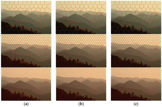
Figure 11. BSLIC superpixels segmentation results. Superpixels number $k=\left[100,500,1000\right]$, weighting factor $m=\left[5,15,30\right]$. (a) BSLIC segments when $m=5$; Column (b) BSLIC segments when $m=15$; Column (c) BSLIC segments when $m=30$.

4.2. Qualitative Comparisons

We compare BSLIC with four other methods: SEEDS, SuperPB, SLIC and Turbopixels. All the 500 images of dataset BSDS500 are segmented by these five methods. As the superpixels are segmented to give a description of features for a subsequent image processing task, they cannot be too small in size. Herein, we maintain the size of a superpixel larger than 80, which is nearly in $9\times 9$ size. For images in $481\times 321$ resolution, when the number of superpixels $k$ exceeds 2000, the generated superpixels are approximately an average size of 77. Therefore, during the experiments, $k$ takes its value at intervals of 100 from 50 to 2500. Weighting factor $m$ is within the range of $\left[5,15,30\right]$.

Figure 12 displays part of the experimental results. The number of superpixels is the same or approximate in every row. Column (a) gives a qualitative presentation for BSLIC segmentations over the whole image domain. The superpixels are compact and uniform hexagons in shape, which is benefits from initializing centers in the hexagon distribution. The superpixels are also regular in size, which is attributed to the locality of k-means clustering. Although SLIC segmentations over the whole image domain are not displayed here, it is necessary to mention that both SLIC and BSLIC superpixels are regular and compact in size and shape. Columns (b)–(f) provide the partial enlarged results of the solid rectangle tagged regions, which contain image edges. Compared with the other four methods, BSLIC superpixels achieve higher adherence to image edges. For the other four methods, we draw conclusions as follows: (1) SEEDS is highly irregular in size and shape; (2) SuperPB has high regularity and compactness in both size and shape, but it lacks flexibility when it comes to the regions containing edges; (3) SLIC and Turbopixel have an equal regularity in size and shape, but their boundary adherences are lower than BSLIC.

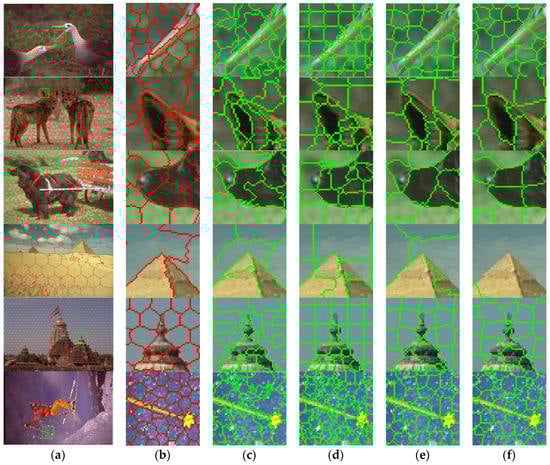
Figure 12. Part of experimental results. (a) BSLIC segments; (b) Partial enlarged superpixels of BSLIC; (c) Partial enlarged superpixels of SEEDS; (d) Partial enlarged superpixels of SuperPB; (e) Partial enlarged superpixels of SLIC; (f) Partial enlarged superpixels of Turbopixles.

4.3. Quantitative Comparisons

The performance metrics of superpixel segmentation methods are different from that of image segmentation and other visual tasks [29]. Recall is a professional index in information retrieval. Boundary recall (BR) was first adopted to measure the accuracy of image segmentation in [1]. Under segmentation error (UE) is another metric to measure the error rate of image segmentation. BR and UE are widely used to measure the boundary adherence of superpixels, which can be demonstrated by [3,15,21,22]. BR and UE measure the boundary adherence in boundary-wise and region-wise situations, respectively. BR is the fraction of ground truth edges that are retrieved by superpixel boundaries within a small neighboring region. The radius of the neighboring region is denoted as $\mathsf{\sigma }$, which is equal to 1 or 2 in the work. UE is the fraction of superpixel regions across ground truth edge. To represent the image more faithfully, high BR and low UE are usually expected. Given the set of superpixel boundaries $\mathrm{Res}$, and the set of ground truth edges $\mathrm{Grd}=\left\{Gr{d}_1,Gr{d}_2,\dots ,Gr{d}_M\right\}$, where $Gr{d}_1,Gr{d}_2,\dots ,Gr{d}_M$ refer to the $M$ ground truth edge images, BR can be expressed as

$$\mathrm{BR}=\frac{1}{M}{\displaystyle \sum }_{m=1}^M\frac{\left|Res{{\displaystyle \cap }}^{\text{}}Gr{d}_m\right|}{\left|Gr{d}_m\right|}$$

(9)

where the operator $|·|$ denotes the size of an element in pixels, $M$ is 5 on average in database BSDS500. UE can be expressed as

$$\mathrm{UE}=\frac{1}{M}{\displaystyle \sum }_{m=1}^M\left\{\frac{1}{N}\left[{\displaystyle \sum }_{q=1}^Q\left({\displaystyle \sum }_{i:Re{s}_i{{\displaystyle \cap }}^{\text{}}{Q}_q\ne \varnothing }\left|Re{s}_i\right|\right)-N\right]\right\}$$

(10)

where $N$ is the image pixels, $Q$ is the number of segments for one ground truth image, $Re{s}_i$ is one segment for superpixel segmentation results.

As the rounding operation is done when calculating the horizontal and vertical intervals, and the initialized centers are updated as the lowest gradient position in a corresponding $3\times 3$ local neighborhood, the numbers of actually generated superpixels $k^{\prime }$ are not equal to $k$. Figure 13 displays the UE curves against $k^{\prime }$. Obviously, BSLIC has lower UE than in the other methods. According to the obtained UE, the boundary adherence can be sorted from high to low as: BSLIC > SEEDS > SuperPB > SLIC > Turbopixels. Figure 14a,b displays the BR curves with radius of neighborhood $\mathsf{\sigma }=1,2$ respectively. It is observed that BSLIC produces a uniform increase for BR when compared with SuperPB, SLIC and Turbopixels. BSLIC is a little bit inferior to SEEDS in boundary recall. However, BSLIC has apparent advantages over SEEDS in the regularity and compactness in size and shape.

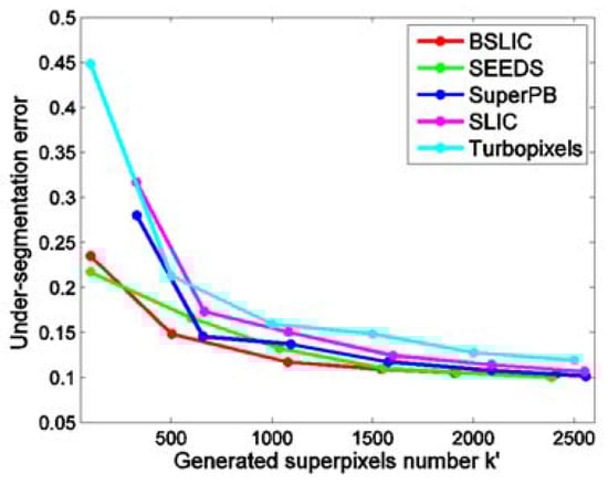
Figure 13. Under segmentation error.

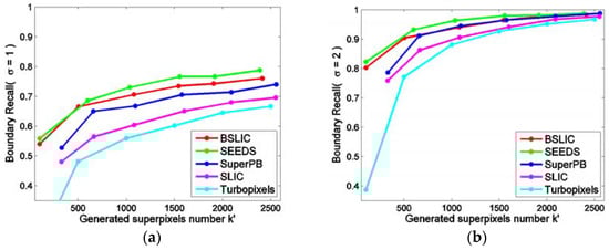
Figure 14. Boundary recall. (a) $\mathsf{\sigma }=1$; (b) $\mathsf{\sigma }=2$.

BSLIC is a modified SLIC method, and a specific comparison between the two methods are conducted. The experimental data are listed in Table 1 and Table 2. Table 1 is the data of $\mathrm{BR}$ with $\mathsf{\sigma }=1$. The generated number of superpixels $k^{\prime }$ is set in the range of $\left[500,1000,1500,2000,2500\right]$, and $m$ is $\left[5,15,30\right]$. For boundary recall, Table 1 shows that BSLIC can achieve at most a 6.23%, 8.56% and 12.43% increase when $m$ is 5, 15 and 30. For under segmentation error, Table 2 shows that BSLIC can achieve at most a 1.46%, 2.77% and 3.51% decrease when $m$ is 5, 15 and 30.

Table 1. Experimental data of $\mathrm{boundary}\mathrm{recall}\left(\mathrm{BR}\right)$.

${\mathit{k}}^{\prime }$		500	1000	1500	2000	2500
$\mathrm{m}=5$	SLIC	0.5932	0.6346	0.6245	0.6791	0.6782
	BSLIC	0.5849	0.6858	0.6888	0.6981	0.7193
	Improving Rate	−0.0083	0.0512	0.0623	0.0190	0.0411
$\mathrm{m}=15$	SLIC	0.5646	0.6035	0.6504	0.6798	0.6957
	BSLIC	0.6501	0.6672	0.7055	0.7139	0.7397
	Improving Rate	0.0856	0.0638	0.0552	0.0340	0.0440
$\mathrm{m}=30$	SLIC	0.5014	0.5500	0.6046	0.6470	0.6793
	BSLIC	0.6257	0.6613	0.6786	0.7042	0.7222
	Improving Rate	0.1243	0.1113	0.0740	0.0572	0.0430

Table 2. Experimental data of under segmentation error $(\mathrm{UE})$.

${\mathit{k}}^{\prime }$		500	1000	1500	2000	2500
$\mathrm{m}=5$	SLIC	0.2146	0.1540	0.1455	0.1247	0.1170
	BSLIC	0.2348	0.1395	0.1334	0.1204	0.1113
	Improving Rate	−0.0202	0.0146	0.0121	0.0043	0.0057
$\mathrm{m}=15$	SLIC	0.1731	0.1505	0.1242	0.1140	0.1064
	BSLIC	0.1415	0.1369	0.1172	0.1078	0.1012
	Improving Rate	0.0277	0.0136	0.0071	0.0062	0.0051
$\mathrm{m}=30$	SLIC	0.1936	0.1572	0.1307	0.1193	0.1090
	BSLIC	0.1585	0.1346	0.1176	0.1067	0.1036
	Improving Rate	0.0351	0.0227	0.0130	0.0126	0.0053

5. Conclusions

This paper presents a superpixel method that achieves an excellent compromise between the boundary adherence and the regularity in size and shape. By initializing cluster centers in a hexagon distribution and initializing the “edge center” as an exact edge pixel, the symmetry properties of superpixels are evidently reduced, which can effectively improve the boundary adherence of edge-across superpixels. With the boundary term being incorporated into the distance calculation of clustering, the boundary adherence of superpixels generated by BSLIC is further improved. Compared with SLIC, the segmentation quality of BSLIC is increased by at most 12.43% for boundary recall and 3.51% for under segmentation error. Based on local k-means clustering, BSLIC superpixels are more regular in size and more compact in shape than the state-of-art methods. One of our future research projects is to apply the BSLIC method to the two-stage semantic image segmentation models.

References

- Ren, X.; Malik, J. Learning a classification model for segmentation. In Proceedings of the IEEE International Conference on Computer Vision (ICCV), Nice, France, 13–16 October 2003.
- Veksler, O.; Boykov, Y.; Mehrani, P. Superpixels and Supervoxels in an Energy Optimization Framework. In Proceedings of the European Conference on Computer Vision-Part V (ECCV Part V), Crete, Greece, 5–11 September 2010.
- Achanta, R.; Shaji, A.; Smith, K.; Lucchi, A.; Fua, P.; Susstrunk, S. SLIC Superpixels Compared to State-of-the-Art Superpixel Methods. IEEE Trans. Pattern Anal. 2012, 34, 2274–2282. [Google Scholar] [CrossRef] [PubMed]
- Li, Z.; Wu, X.M.; Chang, S.F. Segmentation using superpixels: A bipartite graph partitioning approach. In Proceedings of the IEEE International Conference on Computer Vision and Pattern Recognition (CVPR), Providence, RI, USA, 16–21 June 2012.
- Gonzalo-Martín, C.; Lillo-Saavedra, M.; Menasalvas, E.; Fonseca-Luengo, D.; García-Pedrero, A.; Costumero, R. Local optimal scale in a hierarchical segmentation method for satellite images. J. Intell. Inf. Syst. 2016, 46, 517–529. [Google Scholar] [CrossRef]
- Schick, A.; Bauml, M.; Stiefelhagen, R. Improving foreground segmentations with probabilistic superpixel Markov random Fields. In Proceedings of the IEEE International Conference on Computer Vision and Pattern Recognition Workshop (CVPR Workshop), Providence, RI, USA, 16–21 June 2012.
- O, N.K.; Kim, C. Unsupervised Texture Segmentation of Natural Scene Images Using Region-based Markov Random Field. J. Signal Process. Syst. 2016, 83, 423–436. [Google Scholar] [CrossRef]
- Ayvaci, A.; Soatto, S. Motion segmentation with occlusions on the superpixel graph. In Proceedings of the IEEE International Conference on Computer Vision Workshop (ICCV Workshop), Kyoto, Japan, 27 September–4 October 2009.
- Lee, T.; Fidler, S.; Levinshtein, A.; Sminchisescu, C.; Dickinson, S. A Framework for Symmetric Part Detection in Cluttered Scenes. Symmetry 2015, 7, 1333–1351. [Google Scholar] [CrossRef]
- Fu, K.; Gong, C.; Yang, J.; Zhou, Y.; Gu, I.Y.H. Superpixel based color contrast and color distribution driven salient object detection. Signal Process.-Image 2013, 28, 1448–1463. [Google Scholar] [CrossRef]
- Xie, Y.; Lu, H.; Yang, M.H. Bayesian Saliency via Low and Mid-Level Cues. IEEE Trans. Image Process. 2013, 22, 1689–1698. [Google Scholar] [PubMed]
- Peng, H.; Bing, L.; Ling, H.; Hu, W.; Xiong, W.; Maybank, S.J. Salient object detection via structured matrix decomposition. IEEE Trans. Pattern Anal. 2016, 99, 796–802. [Google Scholar] [CrossRef] [PubMed]
- Feng, J.; Cao, Z.; Pi, Y. Polarimetric Contextual Classification of PolSAR Images Using Sparse Representation and Superpixels. Remote Sens. 2014, 6, 7158–7181. [Google Scholar] [CrossRef]
- Garcia-Pedrero, A.; Rodríguez-Esparragón, D.; Gonzalo-Martín, C.; Ibarrola, E.; Lillo-Saavedra, M.; Marcello, J. Automatic identification of shrub vegetation of the Teide National Park. In Proceedings of the International Work Conference on Bio-Inspired Intelligence (IWOBI), San Sebastian, Spain, 10–12 June 2015.
- Bergh, M.V.D.; Boix, X.; Roig, G.; Capitani, B.; Gool, L.V. Seeds: Superpixels extracted via energy-driven sampling. Int. J. Comput. Vis. 2015, 111, 1–17. [Google Scholar]
- Shi, J.; Malik, J. Normalized Cuts and Image Segmentation. IEEE Trans. Pattern Anal. 2000, 22, 888–905. [Google Scholar]
- Pedro, F.; Felzenszwalb, P.F.; Daniel, P.H. Efficient Graph-Based Image Segmentation. Int. J. Comput. Vis. 2004, 59, 167–181. [Google Scholar]
- Thomas, H.C.; Charles, E.L.; Ronald, L.R.; Clifford, S. Introduction to Algorithms, 3rd ed.; The MIT Press: Cambridge, MA, USA, 2009; pp. 43–45. [Google Scholar]
- Comaniciu, D.; Meer, P. Mean Shift: A robust approach toward feature space analysis. IEEE Trans. Pattern Anal. 2002, 24, 603–619. [Google Scholar] [CrossRef]
- Vedaldi, A.; Soatto, S. Quick Shift and Kernel Methods for Mode Seeking. In Proceedings of the European Conference on Computer Vision-Part IV (ECCV Part IV), Marseille, France, 12–18 October 2008.
- Levinshtein, A.; Stere, A.; Kutulakos, K.N.; Fleet, D.J.; Dickinson, S.J.; Siddiqi, K. TurboPixels: Fast Superpixels Using Geometric Flows. IEEE Trans. Pattern Anal. 2009, 31, 2290–2297. [Google Scholar] [CrossRef] [PubMed]
- Zhang, Y.; Hartley, R.; Mashford, J.; Burn, S. Superpixels via Pseudo-Boolean Optimization. In Proceedings of the International Conference on Computer Vision (ICCV), Barcelona, Spain, 6–13 November 2011.
- Liu, Y.J.; Yu, C.C.; Yu, M.J.; He, Y. Manifold SLIC: A Fast Method to Compute Content-Sensitive Superpixels. In Proceedings of the IEEE International Conference on Computer Vision and Pattern Recognition (CVPR), Seattle, WA, USA, 27–30 June 2016.
- Fowlkes, C.; Martin, D.; Malik, J. Learning affinity functions for image segmentation: Combining patch-based and gradient-based approaches. In Proceedings of the IEEE International Conference on Computer Vision and Pattern Recognition (CVPR), Madison, WI, USA, 16–22 June 2003.
- Garcia-Pedrero, A.; Gonzalo-Martin, C.; Fonseca-Luengo, D.; Lillo-Saavedra, M. A GEOBIA methodology for fragmented agricultural landscapes. Remote Sens. 2015, 7, 767–787. [Google Scholar] [CrossRef]
- The Berkeley Segmentation Dataset and Benchmark. Available online: https://www2.eecs.berkeley.edu/Research/Projects/CS/vision/bsds/ (accessed on 24 November 2016).
- Luxburg, U. A tutorial on spectral clustering. Stat. Comput. 2007, 17, 395–416. [Google Scholar] [CrossRef]
- Peng, X.; Tang, H.; Zhang, L.; Zhang, Y.; Xiao, S. A Unified Framework for Representation-Based Subspace Clustering of Out-of-Sample and Large-Scale Data. IEEE Trans. Neural Netw. 2016, 27, 2499–2512. [Google Scholar] [CrossRef] [PubMed]
- Liu, M.Y.; Tuzel, O.; Ramalingam, S.; Chellappa, R. Entropy rate superpixel segmentation. In Proceedings of the IEEE International Conference on Computer Vision and Pattern Recognition (CVPR), Colorado Springs, CO, USA, 20–25 June 2011.
© 2017 by the authors. Licensee MDPI, Basel, Switzerland. This article is an open access article distributed under the terms and conditions of the Creative Commons Attribution (CC BY) license ( http://creativecommons.org/licenses/by/4.0/).