Article

Retinal Vessel Segmentation via Structure Tensor Coloring and Anisotropy Enhancement

1
Department of Computer Engineering, Dicle University, 21280 Diyarbakır, Turkey
2
Department of Electrical and Electronics Engineering, Dicle University, 21280 Diyarbakır, Turkey
*
Author to whom correspondence should be addressed.
Symmetry 2017, 9(11), 276; https://doi.org/10.3390/sym9110276
Submission received: 23 October 2017 / Revised: 9 November 2017 / Accepted: 10 November 2017 / Published: 14 November 2017

Abstract

:
Retinal vessel segmentation is one of the preliminary tasks for developing diagnosis software systems related to various retinal diseases. In this study, a fully automated vessel segmentation system is proposed. Firstly, the vessels are enhanced using a Frangi Filter. Afterwards, Structure Tensor is applied to the response of the Frangi Filter and a 4-D tensor field is obtained. After decomposing the Eigenvalues of the tensor field, the anisotropy between the principal Eigenvalues are enhanced exponentially. Furthermore, this 4-D tensor field is converted to the 3-D space which is composed of energy, anisotropy and orientation and then a Contrast Limited Adaptive Histogram Equalization algorithm is applied to the energy space. Later, the obtained energy space is multiplied by the enhanced mean surface curvature of itself and the modified 3-D space is converted back to the 4-D tensor field. Lastly, the vessel segmentation is performed by using Otsu algorithm and tensor coloring method which is inspired by the ellipsoid tensor visualization technique. Finally, some post-processing techniques are applied to the segmentation result. In this study, the proposed method achieved mean sensitivity of 0.8123, 0.8126, 0.7246 and mean specificity of 0.9342, 0.9442, 0.9453 as well as mean accuracy of 0.9183, 0.9442, 0.9236 for DRIVE, STARE and CHASE_DB1 datasets, respectively. The mean execution time of this study is 6.104, 6.4525 and 18.8370 s for the aforementioned three datasets respectively.

1. Introduction

Retinal blood vessel segmentation and extraction of different features based on these vessel segments, such as tortuosity, width, length, angle and color are exploited for diagnosis and screening of numerous kinds of diseases such as diabetic retinopathy (DR), arteriosclerosis, hypertension, retinopathy of prematurity and choroidal neovascularization [1,2]. The retinal vessel segmentation is also a useful tool for computer-assisted surgery, multimodal image registration and biometric person identification [2,3,4,5]. Manual segmentation of retinal blood vessels is a time-consuming, subjective and boring task which must be performed by trained physicians. The medical community generally admits that the retinal vessel segmentation is one of the basic steps for the development of the retinal disease diagnosis systems [6,7]. A great number of studies related to retinal vessel segmentation have been published previously and these studies can be categorized into 3 main classes as kernel, classifier and tracking-based studies [7].
Kernel-based studies convolve the image with the kernels having different orientations and sizes. Nonetheless, this type of studies needs long execution times when the kernels get larger and have to be applied with more than one orientation. In addition to these, the response of a specific kernel fits with only the vessels whose standard deviation resemble to Gaussian function of that kernel. Thus, the vessels which have unrelated profiles may not be detected by the kernel-based methods [6]. In order to segment the retinal vessels, Chaudhuri et al. came up with a Gaussian function-based two-dimensional linear kernel [8]. Hoover et al. performed vessel segmentation by merging local and region-based features of the retinal vessels via applying a threshold probing technique on the response image of a matched filter [9]. Gang et al. detected retinal vessels by using a second order Gaussian filter whose amplitude is modified [10]. Jiang and Mojon tried to detect the vessels via an adaptive local thresholding scheme using a verification-based multi-threshold probing framework [11]. Al-Rawi et al. enhanced Chaudhuri et al.’s matched filter by using optimized parameters derived from an exhaustive search optimization step [8,12]. Cinsdikici and Aydin offered a retinal vessel segmentation method which is a combination of the matched filter and the ant colony algorithm [13,14]. Zhang et al. performed retinal vessel segmentation by an extended version of the matched filter which exploits the symmetric cross sectional property of the vessels [15].
Classifier-based studies extract a feature vector and classify each pixel as vessel or non-vessel. The supervised and unsupervised methods were applied by the classifier-based studies. Nekovei and Ying offered a backpropagation Artificial Neural Network (ANN) for retinal vessel segmentation in angiography images [16]. Sinthanayothin et al. proposed principal component analysis (PCA) and ANN for the detection of the optic disc, fovea, and retinal vessels [17]. Niemeijer et al. offered a featured a vector for each pixel by exploiting the information from the green channel of the image and using the first and second order derivatives of Gaussian function-based matched filters having various scales [18]. Later, Niemeijer classified the pixels using the k-Nearest Neighbor (k-NN) algorithm [18,19]. Soares et al. segmented the vessels via 2-D Gabor wavelet and supervised classification [20]. Ricci and Perfetti classified the retinal vessel pixels using Support Vector Machine (SVM) and a feature vector composed by using line operators [21]. Marin et al. proposed a retinal vessel segmentation method by classifying a 7-D feature vector derived from gray-level and moment invariant-based features via ANN [22]. Tolias and Panas segmented vessels in the retinal angiogram images via a fuzzy C-means (FCM) clustering algorithm [23]. Simo and de Ves segmented arteries, veins and the fovea in the retinal angiograms by using the Bayesian image analysis [24]. Salem et al. offered a RAdius-based Clustering ALgorithm (RACAL) which uses a distance-based criterion in order to depict the distributions of the image pixels [25]. Villalobos-Castaldi et al. segmented the vessels by using the texture information by merging the gray-level co-occurrence matrix (GLCM) and the local entropy data [26].
Tracking-based studies start vessel tracking from at least one seed point and aim to trace whole vascular pattern step by step. This seed point may be set manually by user or automatically via morphological operations [7]. This type of technique may be disadvantageous because the seed point requirement may cause the study remain as semi-automatic and missing any bifurcation point may result to lose the entire branch [6]. Chutatape et al. performed the segmentation by tracking the vessels using Gaussian and Kalman filters [27]. Quek and Kirbas offered a wave propagation and traceback mechanism which labels each pixel’s vesselness likelihood by using a dual-sigmoidal filter [28]. Delibasis et al. proposed a vessel tracking algorithm which utilizes a parametric model of a vessel composed of a stripe [29].
This study can be classified in the kernel-based category because of the Frangi Vesselness Filter (FVF) and Structure Tensor (ST) steps. However, FVF requires only a few different kernels not for different orientations but only for different scales. More and more, ST algorithm has a lightweight time complexity since it does not execute iteratively for various rotations and scales. The novel parts of this algorithm are utilizing ST as a vessel extraction technique followed by combining anisotropy enhancement function and applying Contrast Limited Adaptive Histogram Equalization (CLAHE) and enhanced mean surface curvature (EMSC) multiplication to the energy space of the tensor field as well as exploiting the coloring part of the tensor visualization method as a new segmentation algorithm. Although a great number of methods were developed, new retinal vessel segmentation techniques are needed still [6]. This study proposes a fast method which extracts the main vessel arcs with a high sensitivity and reasonable accuracy. This article is the extended version of a previously presented conference paper [30]. The main contribution of this article is reducing the false positive segmentation results especially occurring on the main vessel arc by using EMSC multiplication and ST instead of improved structure tensor (IST). Apart from that, this study is tested not only on DRIVE dataset but also on STARE and CHASE_DB1 datasets and higher performance results are obtained. Some extra post-processing steps such as lesion removal and small hole filling are also added to this study.

2. Materials and Methods

2.1. Materials

The DRIVE dataset contains 40 images which are captured via a Canon CR5 non-mydriatic 3CCD camera with a 45-degree field of view (FOV) having an approximately diameter of 540 pixels. 7 of the images have mild early DR. The manual ground truth segmentation and the mask image corresponding to the FOV are given for each image [31].
The STARE dataset contains 20 images which are captured using a TopCon TRV-50 fundus camera at 35 degree FOV having an approximate diameter of 650 × 500 pixels and 10 of these images include pathology [9].
The CHASE_DB1 dataset contains 28 images which are captured at 30 degree FOV with a resolution of 1280 × 960 pixels from 14 patients in Child Heart And Health Study in England [32].

2.2. Methods

The main flowchart of the algorithm is depicted in Figure 1.

2.2.1. Frangi Vesselness Filter

FVF is an algorithm to enhance vessels or tubular structures in medical images which may have different modalities. The Hessian matrix of the target image which is symbolized by H can be obtained via second order Gaussian derivative of image f at point x and scale σ as it is shown Equation (1).
H = d 2 I σ d x 2 = f ( x ) *   d 2 G ( σ , x ) d x 2
The sorted λ1 and λ2 Eigenvalues of Hessian matrix of a 2-D image are shown in Equation (2).
| λ 1 |   | λ 2 |
Frangi, defined two new metrics for 2-D images as S and RB to measure the background noise in images and the digression from a blob-like structure, respectively. These two metrics are shown Equation (3).
R B = | λ 1 | / | λ 2 | S = H F = i λ i 2
The vesselness function V F r a n g i which uses the aforementioned metrics is shown in Equation (4) where β and c are real positive and user defined parameters [33].
V F r a n g i ( σ , x ) = { e x p ( R B 2 2 β 2 ) ( 1 e x p ( S 2 2 c 2 ) )
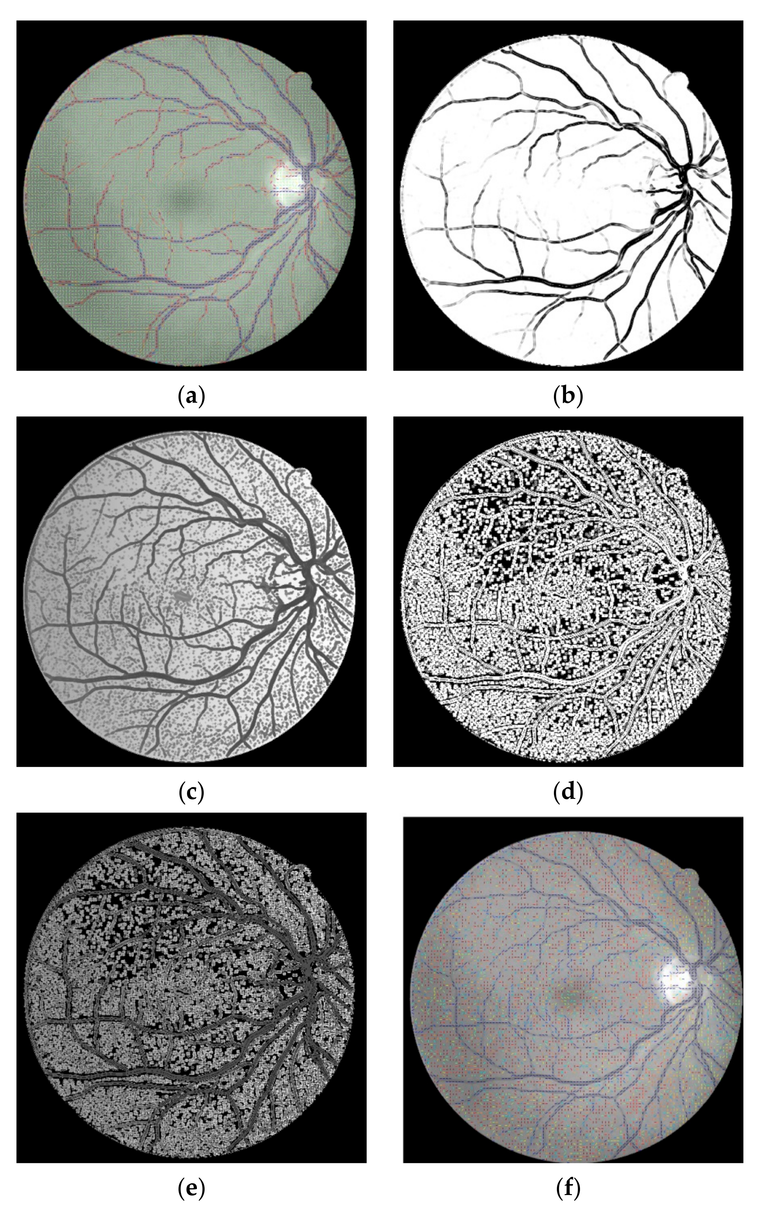
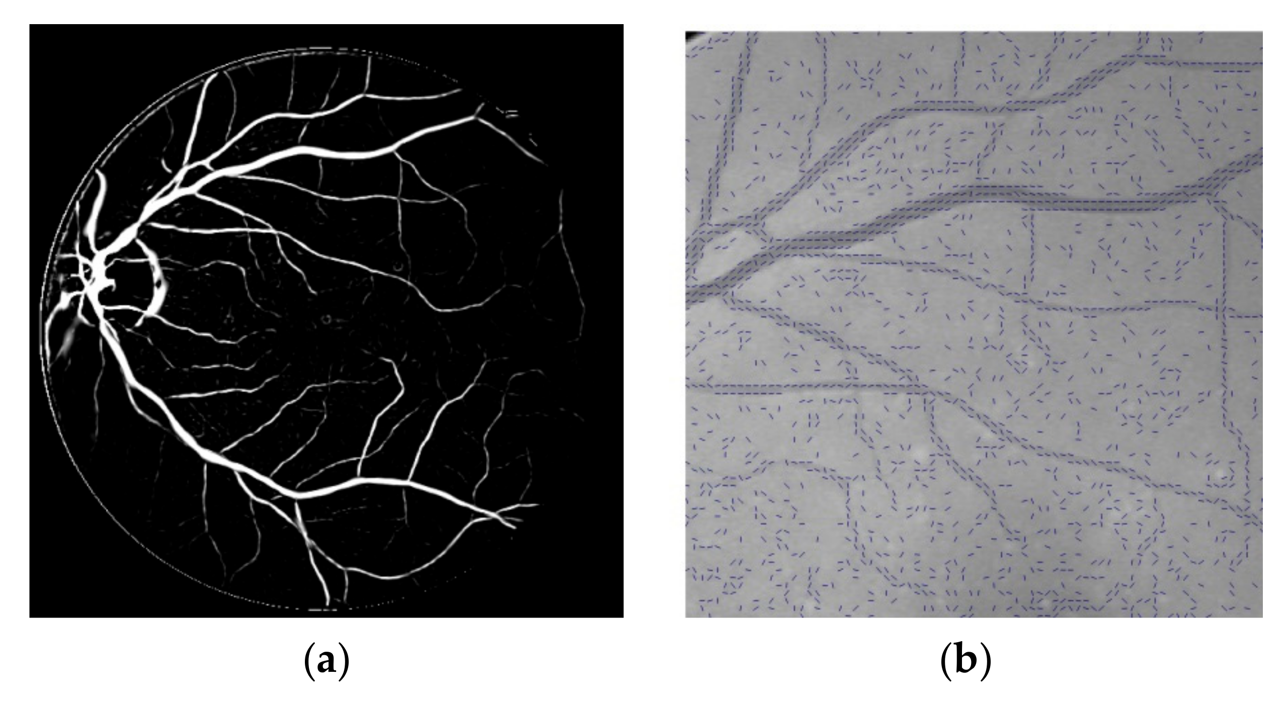
FVF is applied to images in order to emphasize all the retinal vessels with respect to the background. The β and c are set as 0.5 and 15 respectively. The scale range is determined as between 0.01 and 7.01 increasing by 0.5 for each scale. The enhanced filter response of FVF is shown in Figure 2a.

2.2.2. Structure Tensor

ST is basically a covariance matrix which is composed of the partial derivatives of gradients across the edges [34,35]. One of the most important benefits of ST is the coherence concept which is calculated via its Eigenvalues. ST has been used for low-level feature analysis such as feature extraction, edge and corner detection after it was introduced by Förstner as well as Harris and Stevens [32,35,36]. In the literature, there are basically linear and nonlinear types of ST [37,38]. Both types apply smoothing functions or kernels to the basic form of ST which is the covariance matrix of the gradients. Smoothing the ST via Gaussian is a common approach [37]. However, the smoothing operation also blurs the edge information as a side effect. In this study, ST is used solely without applying any linear or nonlinear functions since the fact that it is observed the blurring effect highly increases the false positives in the case of retinal vessel segmentation.
ST is an array of (2,2) which is composed of x and y edge derivatives of image f which is an array of (m,n). ST is calculated for each pixel of the image as in Equation (5) and a tensor field which is an array of size (m,n,2,2) is obtained.
S T =   ( f x 2 f x f y f x f y f y 2 )
A frame of the result of the ST is visualized via tensor visualization technique using ellipsoids as shown in Figure 2b. The size of the ellipsoid visualization field is set as (m/3,n/3,2,2) in order to get a basic idea about the structure of the tensor field. The flow of the sticky ellipsoids depicts the tensors which reside on the vessels while the blob-like ellipsoids represent the non-vessel region.

2.2.3. Anisotropy Enhancement Using Principal Eigenvalue

The contrast between vessel and non-vessel tensors on the obtained tensor field via ST is proposed to be improved by enhancing the anisotropy between the principal Eigenvalues. The λ1 and λ2 of the tensor field is obtained as arrays of (m,n,1). It is seen that contrast between the Eigenvalues of each tensor is not high enough and an enhancement function Z is applied to the principal Eigenvalue λ1 as it is shown in Equation (6). The values of ε and α are set experimentally as 0.001 and −50 respectively. The result of the anisotropy enhancement is visualized via ellipsoids again as it is shown in Figure 3a [39].
λ 1 = Z ( λ 1 ) Z ( λ 1 ) =   ( λ 1 + ε ) α

2.2.4. Applying CLAHE to Energy of Tensor Field

At this step, the energy, anisotropy and orientation of the resulting tensor field is calculated for each pixel using the resulting anisotropy enhanced ST field (AEST) as in Equation (7). The, b and c symbols in Equation (7) define the elements of the AEST tensor field for each pixel. In order to increase the contrast of the vessels a little bit more, CLAHE algorithm is applied to the obtained energy matrix [40]. The energy, anisotropy and orientation values for each pixel are calculated using the values of the matrix elements of the corresponding tensors as in Equation (7). The before and after effect of CLAHE over the energy matrix is shown in Figure 3b,c.
A E S T = ( a c c b ) , E n e r g y = a + b A n i s o t r o p y = 4 ( a   b c 2 ) / ( a + b ) 2 O r i e n t a t i o n = a r c t a n   ( 2 c , ( a b ) ) 2

2.2.5. Enhanced Mean Surface Curvature Multiplication

An infinite number of curves can be drawn on a point of a continuous surface M which can be parametrized by u and v axes. The curvature value at a certain point of each curve C is calculated using the second derivative of its arc length parametrization which is symbolized by C″(s). The normal curvature, Kn, on a certain point of a curve C is calculated by projecting C″(s) onto the normal vector N at that point as in Equation (8). The maximum and minimum normal curvature values for each point on a surface M are called as principal curvatures and shown as k1 and k2 as in Equation (9). The first fundamental form variables are shown as E, F and G as in Equation (10) whereas the second fundamental form variables are shown as e, f and g as in Equation (11) using partial derivatives of surface M. The continuous calculation of Gaussian and mean surface curvatures which are respectively shown as K and H are given as in Equation (12). The discrete calculation of K and H are shown as in Equation (13). The discrete recalculation of k1 and k2 is shown in Equation (14) [41].
K n =   C ( s ) ,   N
k 1 = max ( K n )   ,     k 2 = min ( K n )  
E = M u   M u   ,     F = M u   M v   ,     G = M v   M v  
n =   M u   x   M v ( M u   x   M v ) 2 ,     e = M u u   n   ,     f = M u v   n   ,     g = M v v   n  
H = ( k 1 + k 2 ) 2   ,     K =   k 1   k 2  
H = e G + g E 2 f F 2 ( E G F 2 ) ,     K = e g f 2 E G F 2  
k 1 = H +   H 2 K ,       k 2 = H   H 2 K  
At this step of the study, the CLAHE applied energy space is modeled as a surface in order to enhance the segmentation results by reducing false positive pixels via mean surface curvature information. Firstly, the discrete versions of K, H, k1 and k2 are calculated and then EMSC is calculated using γ which is experimentally set as 10 as in Equation (15). Then, it is converted to binary form via decomposing the positive and negative valued pixels which are respectively shown as p and q symbols as in Equation (16). Afterwards, the formerly CLAHE applied Energy space is multiplied by EMSC as in Equation (19).
E M S C = ( k 1   ×   γ + k 2 ) 2
p i , j ,   q i , j   E M S C ,     q i , j   > 0 ,       p i , j   0 ,     E M S C ( q i , j ) 1 ,     E M S C ( p i , j ) 0 ,
E n e r g y = ( E n e r g y ) ( E M S C )
At the end, the histogram equalized and EMSC multiplied energy matrix is embedded back to the CLAHE applied AEST tensor field (CAEST) again via Eigen recomposition steps as shown in Equation (18) and Figure 3f [42]. The a′, b′ and c′ symbols in Equation (18) define the final values of the elements of the CAEST tensor field for each pixel.
P =   ( E n e r g y ) 2 A n i s o t r o p y 4 D =   ( E n e r g y ) 2 4 P λ 1 =   ( E n e r g y + D   ) 2 λ 2 =   E n e r g y   λ 1 e 1 ( 1 ) = cos   ( O r i e n t a t i o n ) e 1 ( 2 ) = sin ( O r i e n t a t i o n ) e 1 ( 1 ) = sin ( O r i e n t a t i o n ) e 1 ( 2 ) = cos ( O r i e n t a t i o n ) a   =   ( e 1 ( 1 ) ) 2 λ 1 + ( e 2 ( 1 ) ) 2 λ 2 b =   ( e 1 ( 2 ) ) 2 λ 1 + ( e 2 ( 2 ) ) 2 λ 2 c =   e 1 ( 1 ) e 1 ( 2 ) λ 1 + e 2 ( 1 ) e 2 ( 2 ) λ 2 C A E S T   =   ( a c c b )

2.2.6. Tensor Coloring

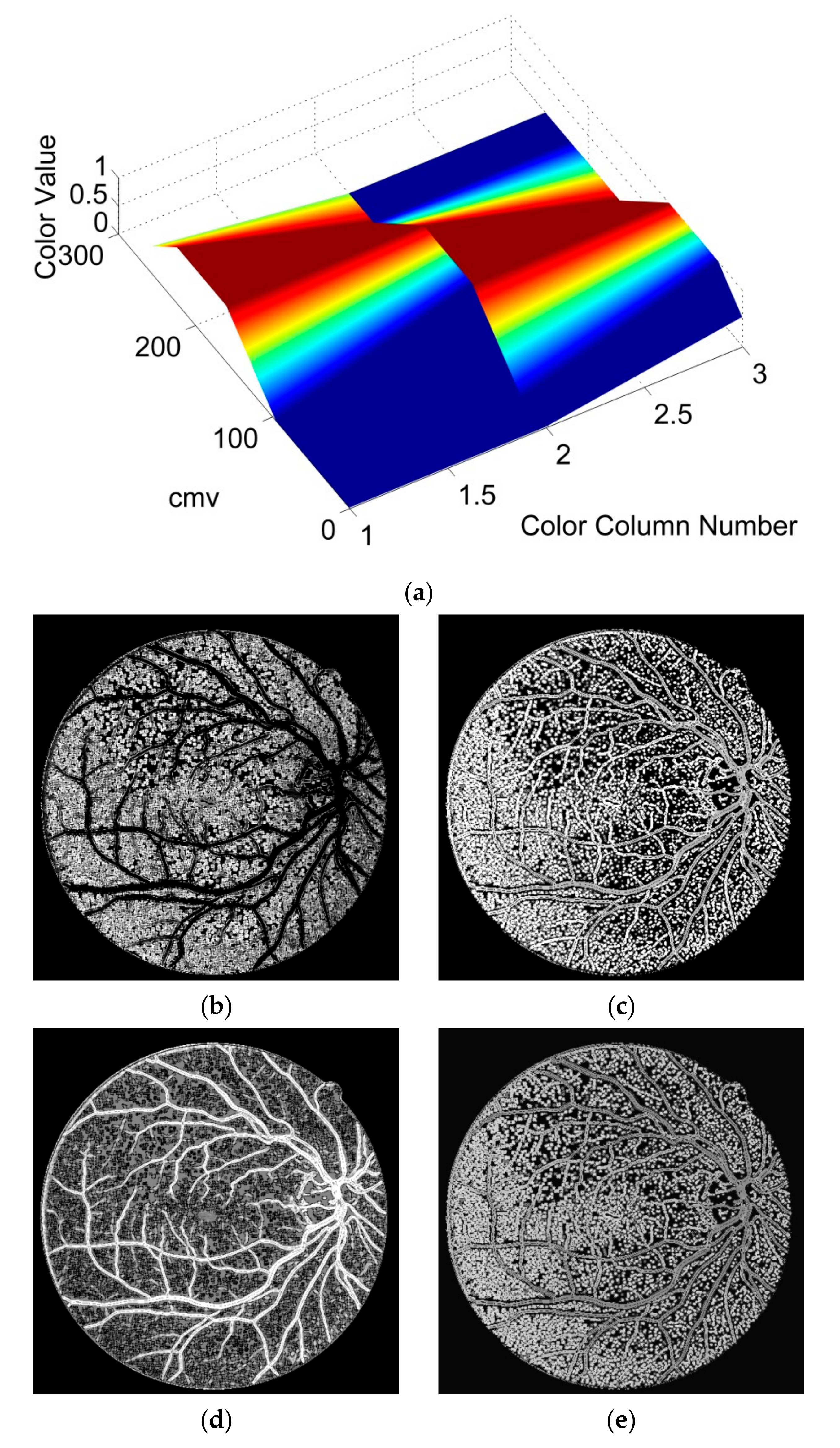
The 4-D tensor fields are able to be visualized using ellipsoids. The radius, orientation and color of the ellipsoids are configured with respect to the values of the tensors. In this study, the tensor coloring method of the visualization technique which uses ellipsoids is exploited as a segmentation method since it can be observed that this visualization technique has a reasonable ability to distinguish the vessel and non-vessel tensors. The tensor coloring procedure is described in Equation (19). Firstly, the maximum and minimum of the sum of diagonal tensor values of CAEST are computed. Then, a color map matrix of (256, 3) is generated in MATLAB as it is shown in Figure 4a. Afterwards, the matrix of color map value which is represented as cmv is calculated and its negative values are set as zero. Thereafter, the corresponding values of cmv with respect to each column of the Map matrix constitutes the Colors1, Colors2 and Colors3 matrixes as can be seen in Figure 4b–d, respectively. Finally, these three color matrixes are merged into Colors matrix using cat command of MATLAB as it is shown as a colorful RGB image in Figure 4e [42].
C A E S T   =   ( a c c b ) m a x i m u m   = m a x ( a + b ) m i n i m u m   = m i n ( a + b ) M a p   =   c o l o r m a p ( j e t ( 256 ) ) c m v   = 255 ( a + b m i n i m u m ) ( m a x i m u m m i n i m u m ) p i     c m v     &     p i < 0 ,   p i   0 C o l o r s 1 =   M a p ( c m v + 1 , 1 ) C o l o r s 2   =   M a p ( c m v + 1 , 2 ) C o l o r s 3 =   M a p ( c m v + 1 , 3 ) C o l o r s = c a t ( C o l o r s 1     C o l o r s 2     C o l o r s 3 )
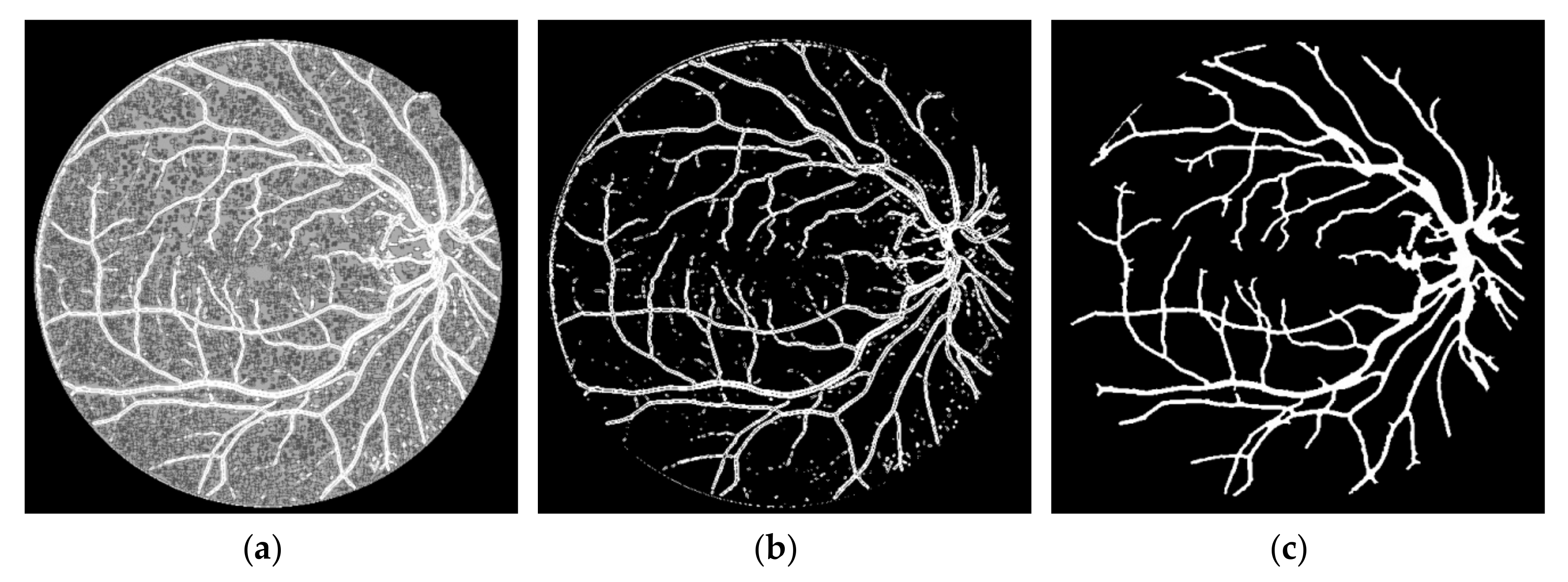
The Colors3 image is selected because of its higher contrast and OTSU method is applied to it in order to determine 3 main gray histogram distributions as it is shown in Figure 5a [43]. Then, the vessels are thresholded and the remaining artifacts such as small unconnected pixels are removed using bwareaopen command of MATLAB. The final segmentation result is shown in Figure 5b,c.

2.2.7. Post-Processing

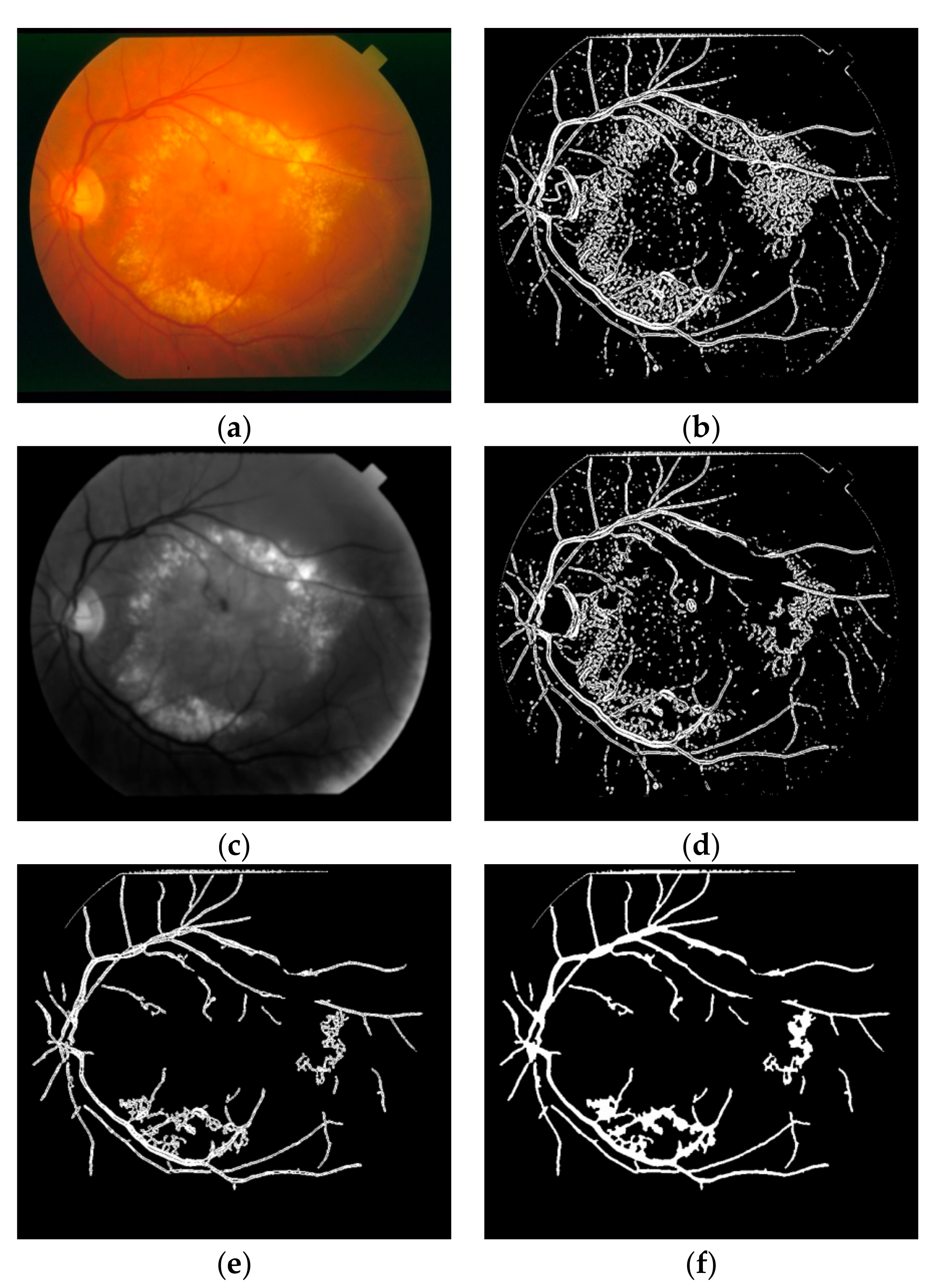
In this study, two different approaches are offered for the lesion removal procedure at the post-processing step. The effects of the post-processing procedures are shown on the segmentation steps of an image having DR in STARE dataset as in Figure 6. The first approach targets especially the spread hard and soft exudate lesions. The highest 10% of the histogram of the product of hue and green color space of the retinal image having these kinds of lesions is removed from the segmentation result as in Figure 6d.
The second approach aims to remove all the other lesions or residual artefacts by taking into account their geometric structures such as solidity and eccentricity. The ratio of the region of a connected component to its convex hull is defined as solidity. The ratio of the distance between the foci of the ellipse which has same the second-moments as a connected component and its major axis length is defined as eccentricity [44]. It was empirically inspected with a high probability that the connected components having solidity value above 0.3 and eccentricity value below 0.95 are lesion. After removing the lesion-like connected components as in Figure 6e, all the residual connected components which are smaller than 100 pixels are deleted from the segmentation result. Finally, the small holes occurring on the vessels because of the central vessel reflex are filled using some successive morphological operations as shown in Figure 6f.

3. Evaluation and Results

Based on the evaluation criteria of the previous retinal vessel segmentation studies, the true positive (TP) is defined as the count of the pixels which are detected as vessel in both the ground truth and segmented images whereas the true negative (TN) is defined as the count of the pixels which are detected as non-vessel in both the ground truth and segmented images. The false positive (FP) is defined as the count of the pixels which are detected as vessel in segmented image but non-vessel in the ground truth image while the false negative (FN) is defined as the count of the pixels which are detected as non-vessel in segmented image but vessel in the ground truth image. The sensitivity (SN) is defined as the ratio of the TP to the sum of TP and FN. The specificity (SP) is defined as the ratio of the TN to the sum of TN and FP. The accuracy (ACC) is defined as the ratio of the sum of the TP and TN to the number of the pixels in the FOV [6]. The area under a receiver operating characteristic curve (AUC) is commonly used for the measuring the performance of the classifiers for different thresholds which is not applicable for unsupervised methods. Another definition such as AUC = (Sensitivity + Specificity)/2 is more suitable for unsupervised methods like the proposed study [45,46].
In this study, the sensitivity, specificity, accuracy, AUC and execution time values for the 40, 20 and 28 images of DRIVE, STARE and CHASE_DB1 datasets are respectively shown in Table 1, Table 2 and Table 3.
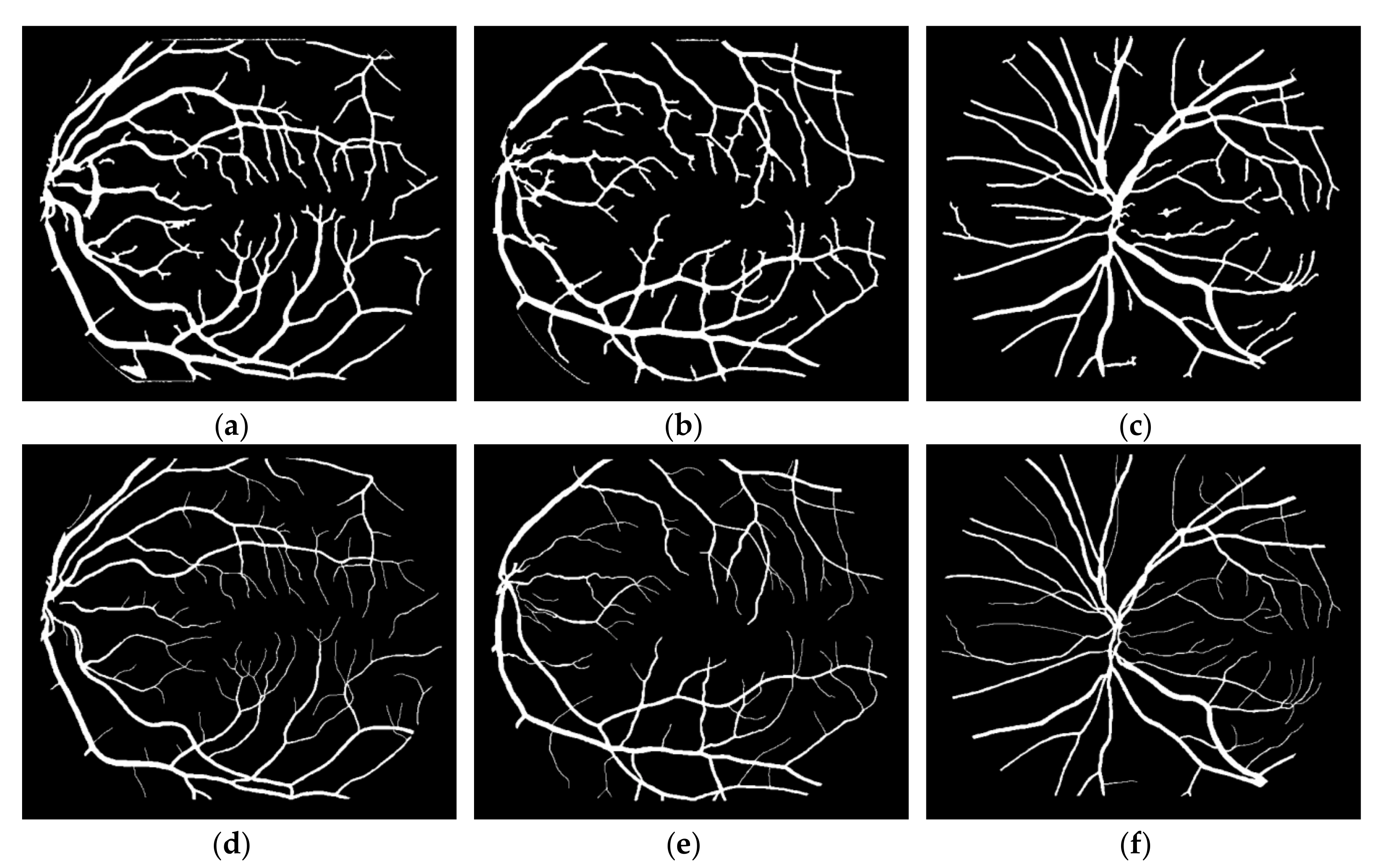
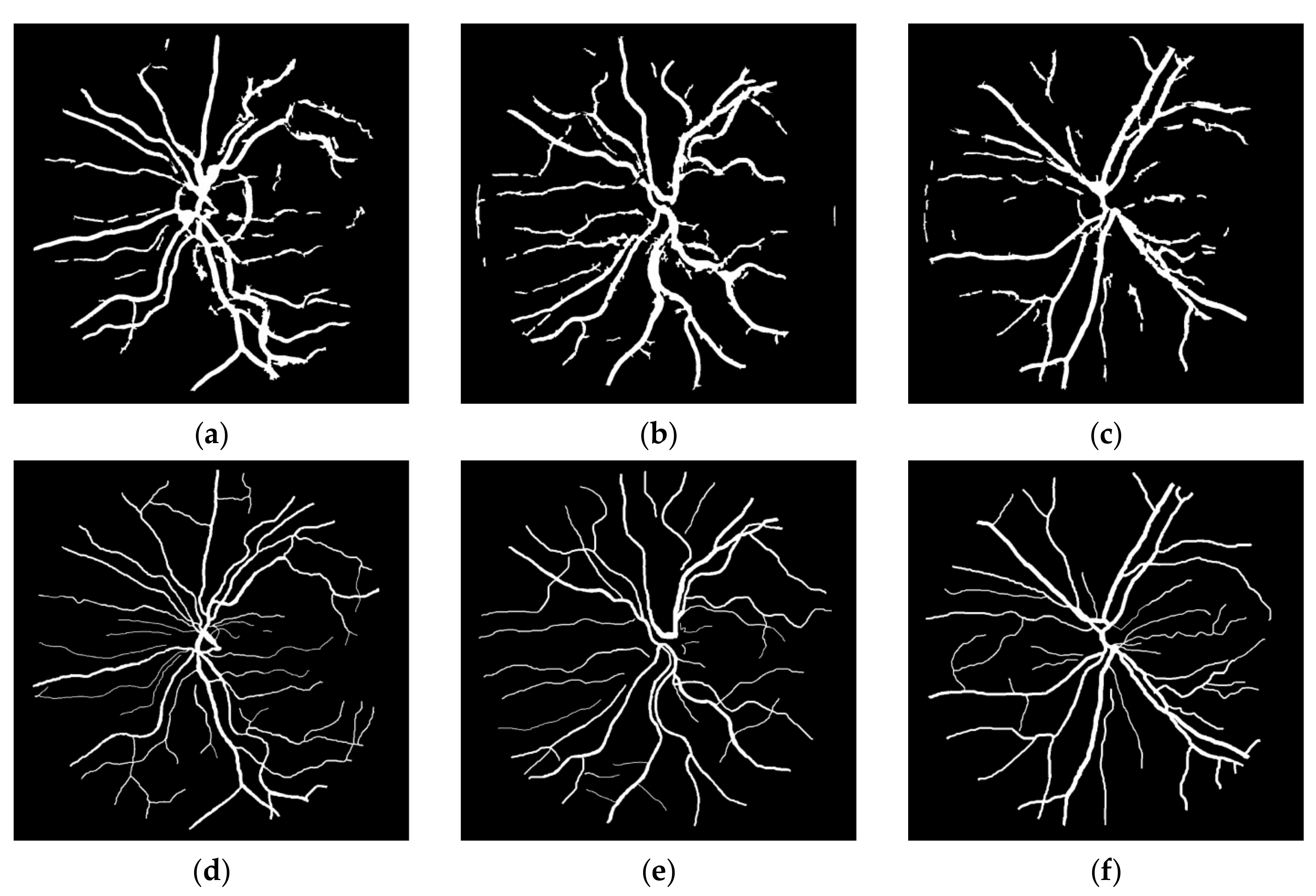
Some of segmentation results and their ground truth images are shown respectively for DRIVE, STARE and CHASE_DB1 datasets in Figure 7, Figure 8 and Figure 9.

4. Discussion

FVF is utilized as a useful preprocessing step in terms of only being able to focus on vessel-like regions. The ST method which is used in this study is successful on the edge extraction by using gradient information. Anisotropy Enhancement step of the 4-D tensor field contributed to vessel enhancement by not deforming the topology of the vessels but only emphasizing the vessel borders and regions. Applying CLAHE to the energy space is useful for normalizing the pixel values after anisotropy enhancement step. The EMSC multiplication step reduces the number of the false positive pixels which reside on the vessel borders even if it also causes a lot of small holes to occur on the vessels which are filled during post-processing. In this study, the proposed lesion removal procedure is also exploited successfully in order to eliminate the miscellaneous artefacts exaggerated by the FVF and ST.
This study does not require parameter calibration except for the parameters of FVF, EMSC and lesion removal criteria as well as can be used automatically for various retinal images having light inhomogeneity and different resolution values. In addition to these, this study offers a new approach for segmentation literature by utilizing tensor visualization technique which uses ellipsoids. As far as we know, this study is the first one in which the tensor coloring method is used for segmentation.
The performance results of the proposed study and the recent state of the art studies in the last two years are compared as in Table 4, Table 5 and Table 6. This study suggests encouraging sensitivity, specificity, accuracy, AUC and execution time results with respect to the literature for DRIVE, STARE and CHASE_DB1 datasets. The performance results of the proposed study and the results of the other studies which are lower than the corresponding evaluation criterion is written as bold in the below tables. The sensitivity of this study is better than [45,47,48,49,50,51,52] whereas its specificity is better than [53] and its accuracy and AUC is respectively more successful than [48] and [45,51] for DRIVE dataset as in Table 4. The sensitivity of this study is more successful than [45,49,51,52,54,55] whereas the performance of its specificity is better than [53,55] and its accuracy and AUC is respectively higher than [48,53,55] and [45,51] for STARE dataset as in Table 5. The performance of the sensitivity of this study is higher than [56] whereas its accuracy is more successful than [57] for CHASE_DB1 dataset as in Table 6. Performance comparison of the average execution times for DRIVE and STARE datasets between this study and some of the state of the art studies are given in Table 7 [52]. The algorithm of this study is implemented in MATLAB and executed in a PC with 2.2 GHz Intel core i7 CPU and 4 GB RAM.
One of the superiorities of this study with respect to the previous studies is its higher sensitivity values by not trading off the specificity and accuracy values dramatically. The other advantage of this study is that, as far as we know, it has the lowest execution time in the literature as shown in Table 7 [52]. The most important reason of the lower AUC values of this study is because of the fact that the previously mentioned calculation method of the AUC for the unsupervised algorithms yields lower values with respect to the supervised methods which can be crosschecked by looking sensitivity, accuracy and AUC values of the studies listed in Table 4, Table 5 and Table 6 [45,46]. The proposed novel ST coloring-based vessel segmentation method can be utilized for different kind of micro tubular segmentation problems. This method can also be easily implemented on parallel software and hardware systems since the fact that the parallelizable structure of the employed tensor operations. The lesion removal algorithm which is proposed in this study can be exploited not only for the retinal image segmentation task but also for the different problems of medical image analysis.
This study can be beneficial for diagnosis of hypertension, retinopathy of prematurity, arteriosclerosis, choroidal neovascularization and diabetic retinopathy by providing the elegant sensitivity, specificity and accuracy metrics as well as execution speed [1,2]. In future, we will optimize all the parameters of this proposed retinal vessel segmentation algorithm via hyper parameter optimization techniques which will definitely improve its accuracy and speed.

5. Conclusions

In this study, the retinal vessel segmentation was performed with mean sensitivity of 0.8123, mean specificity of 0.9342, mean accuracy of 0.9183, mean AUC of 0.8732 and mean execution time of 6.104 s on DRIVE dataset. The vessel segmentation was achieved with mean sensitivity of 0.8126, mean specificity of 0.9442, mean accuracy of 0.9312, mean AUC of 0.8784 and mean execution time of 6.4525 s on STARE dataset.
The vessel detection was performed with mean sensitivity of 0.7246, mean specificity of 0.9453, mean accuracy of 0.9236, mean AUC of 0.8349 and mean execution time of 18.8370 s on CHASE_DB1 datasets. The proposed algorithm provided encouraging results especially by detecting main vessel arcs with reasonable sensitivity, specificity and accuracy values for 3 different publically available datasets and offering a new approach for segmentation literature by exploiting the coloring algorithm of the tensor visualization technique which uses ellipsoids.

Acknowledgments

This research did not receive any specific grant from funding agencies in the public, commercial, or not-for-profit sectors. The authors would like to thank the editors and anonymous reviewers for their helpful comments and suggestions. The authors would also like to thank Gabriel Peyré at the National Center for Scientific Research (CNRS) of France for providing valuable MATLAB codes at the noumerical-tours website [43].

Author Contributions

Mehmet Nergiz utilized the Frangi Vesselness Filter and proposed Structure Tensor, Anisotrophy Enhancement, Histogram Equalization of Energy Field, Enhanced Mean Surface Curvature Multiplication and Tensor Coloring algorithms. Mehmet Akın supervised all the research process and proposed lesion removal algorithms.

Conflicts of Interest

The authors declare that there are no competing interests regarding the publication of this paper.

References

  1. Teng, T.; Lefley, M.; Claremont, D. Progress towards automated diabetic ocular screening: A review of image analysis and intelligent systems for diabetic retinopathy. Med. Biol. Eng. Comput. 2002, 40, 2–13. [Google Scholar] [CrossRef] [PubMed]
  2. Kanski, J.J. Clinical Ophthalmology, 6th ed.; Elsevier Health Sciences: London, UK, 2007. [Google Scholar]
  3. Zana, F.; Klein, J.C. A multimodal registration algorithm of eye fundus images using vessels detection and Hough transform. IEEE Trans. Med. Imaging 1999, 18, 419–428. [Google Scholar] [CrossRef] [PubMed]
  4. Mariño, C.; Penedo, G.; Penas, M.; Carreira, J.; Gonzalez, F. Personal authentication using digital retinal images. Pattern Anal. Appl. 2006, 9, 21–33. [Google Scholar] [CrossRef]
  5. Köse, C.; Ikibas, C. A personal identification system using retinal vasculature in retinal fundus images. Expert Syst. Appl. 2011, 38, 13670–13681. [Google Scholar] [CrossRef]
  6. Fraz, M.M.; Remagninoa, P.; Hoppea, A.; Uyyanonvarab, B.; Rudnickac, A.R.; Owen, C.G.; Barman, S.A. Blood vessel segmentation methodologies in retinal images—A survey. Comput. Methods Programs Biomed. 2012, 108, 407–433. [Google Scholar] [CrossRef] [PubMed]
  7. Kaur, M.; Talwar, R. Review on: Blood Vessel Extraction and Eye Retinopathy Detection. Int. J. Comput. Sci. Inf. Technol. 2014, 5, 7513–7516. [Google Scholar] [CrossRef]
  8. Chaudhuri, S.; Chatterjee, S.; Katz, N.; Nelson, M.; Goldbaum, M. Detection of blood vessels in retinal images using two-dimensional matched filters. IEEE Trans. Med. Imaging 1989, 8. [Google Scholar] [CrossRef] [PubMed]
  9. Hoover, A.D.; Kouznetsova, V.; Goldbaum, M. Locating blood vessels in retinal images by piecewise threshold probing of a matched filter response. IEEE Trans. Med. Imaging 2000, 19, 203–210. [Google Scholar] [CrossRef] [PubMed]
  10. Gang, L.; Chutatape, O.; Krishnan, S.M. Detection and measurement of retinal vessels in fundus images using amplitude modified second-order Gaussian filter. IEEE Trans. Biomed. Eng. 2002, 49, 168–172. [Google Scholar] [CrossRef] [PubMed]
  11. Jiang, X.; Mojon, D. Adaptive local thresholding by verification-based multithreshold probing with application to vessel detection in retinal images. IEEE Trans. Pattern Anal. Mach. Intell. 2003, 25, 131–137. [Google Scholar] [CrossRef]
  12. Al-Rawi, M.; Qutaishat, M.; Arrar, M. An improved matched filter for blood vessel detection of digital retinal images. Comput. Biol. Med. 2007, 37, 262–267. [Google Scholar] [CrossRef] [PubMed]
  13. Marco, D.; Thomas, S. Ant Colony Optimization; Bradford Company: Holland, MI, USA, 2004. [Google Scholar]
  14. Cinsdikici, M.G.; Aydin, D. Detection of blood vessels in ophthalmoscope images using MF/ant (matched filter/ant colony) algorithm. Comput. Methods Programs Biomed. 2009, 96, 85–95. [Google Scholar] [CrossRef] [PubMed]
  15. Zhang, B.; Zhang, L.; Zhang, L.; Karray, F. Retinal vessel extraction by matched filter with first-order derivative of Gaussian. Comput. Biol. Med. 2010, 40, 438–445. [Google Scholar] [CrossRef] [PubMed]
  16. Nekovei, R.; Ying, S. Back-propagation network and its configuration for blood vessel detection in angiograms. IEEE Trans. Neural Netw. 1995, 6, 64–72. [Google Scholar] [CrossRef] [PubMed]
  17. Sinthanayothin, C.; Boyce, J.F.; Cook, H.L.; Williamson, T.H. Automated localisation of the optic disc, fovea, and retinal blood vessels from digital colour fundus images. Br. J. Ophthalmol. 1999, 83, 902–910. [Google Scholar] [CrossRef] [PubMed]
  18. Niemeijer, M.; Staal, J.J.; van Ginneken, B.; Loog, M.; Abramoff, M.D. Comparative study of retinal vessel segmentation methods on a new publicly available database. SPIE Med. Imaging 2004, 648–656. [Google Scholar] [CrossRef]
  19. Shakhnarovic, G.; Darrel, T.; Indyk, P. Nearest-Neighbor Methods in Learning and Vision: Theory and Practice; Neural Information Processing; MIT Press: Cambridge, MA, USA, 2006. [Google Scholar]
  20. Soares, J.V.B.; Leandro, J.J.G.; Cesar, R.M.; Jelinek, H.F.; Cree, M.J. Retinal vessel segmentation using the 2d gabor wavelet and supervised classification. IEEE Trans. Med. Imaging 2006, 25, 1214–1222. [Google Scholar] [CrossRef] [PubMed] [Green Version]
  21. Ricci, E.; Perfetti, R. Retinal blood vessel segmentation using line operators and support vector classification. IEEE Trans. Med. Imaging 2007, 26, 1357–1365. [Google Scholar] [CrossRef] [PubMed]
  22. Marin, D.; Aquino, A.; Gegundez-Arias, M.E.; Bravo Caro, J.M. A new supervised method for blood vessel segmentation in retinal images by using gray-level and moment invariants-based features. IEEE Trans. Med. Imaging 2011, 30, 146–158. [Google Scholar] [CrossRef] [PubMed]
  23. Tolias, Y.A.; Panas, S.M. A fuzzy vessel tracking algorithm for retinal images based on fuzzy clustering. IEEE Trans. Med. Imaging 1998, 17, 263–273. [Google Scholar] [CrossRef] [PubMed]
  24. Simó, A.; de Ves, E. Segmentation of macular fluorescein angiographies. A statistical approach. Pattern Recognit. 2001, 34, 795–809. [Google Scholar] [CrossRef]
  25. Salem, S.; Salem, N.; Nandi, A. Segmentation of retinal blood vessels using a novel clustering algorithm (RACAL) with a partial supervision strategy. Med. Biol. Eng. Comput. 2007, 45, 261–273. [Google Scholar] [CrossRef] [PubMed]
  26. Villalobos-Castaldi, F.; Felipe-Riverón, E.; Sánchez-Fernández, L. A fast, efficient and automated method to extract vessels from fundus images. J. Vis. 2010, 13, 263–270. [Google Scholar] [CrossRef]
  27. Chutatape, O.; Liu, Z.; Krishnan, S.M. Retinal blood vessel detection and tracking by matched Gaussian and Kalman filters. In Proceedings of the 20th Annual International Conference of the IEEE Engineering in Medicine and Biology Society, Hong Kong, China, 29 October–1 November 1998; Volume 3146, pp. 3144–3149. [Google Scholar] [CrossRef]
  28. Quek, F.K.H.; Kirbas, C. Vessel extraction in medical images by wave-propagation and traceback. IEEE Trans. Med. Imaging 2001, 20, 117–131. [Google Scholar] [CrossRef] [PubMed]
  29. Delibasis, K.K.; Kechriniotis, A.I.; Tsonos, C.; Assimakis, N. Automatic model-based tracing algorithm for vessel segmentation and diameter estimation. Comput. Methods Programs Biomed. 2010, 100, 108–122. [Google Scholar] [CrossRef] [PubMed]
  30. Nergiz, M.; Akın, M. Retinal Vessel Segmentation via Tensor Coloring. In Proceedings of the International Engineering, Science and Education Conference, Diyarbakır, Turkey, 1–3 December 2016. [Google Scholar]
  31. Niemeijer, M.; Staal, J.; Ginneken, B.; Loog, M.; Abramoff, M. Drive: Digital Retinal Images for Vessel Extraction, 2004. Available online: http://www.isi.uu.nl/Research/Databases/DRIVE (accessed on 18 October 2017).
  32. Owen, C.G.; Rudnicka, A.R.; Mullen, R.; Barman, S.A.; Monekosso, D.; Whincup, P.H.; Ng, J.; Paterson, C. Measuring retinal vessel tortuosity in 10-year-old children: Validation of the Computer-Assisted Image Analysis of the Retina (CAIAR) Program. Investig. Ophthalmol. Vis. Sci. 2009, 50, 2004–2010. [Google Scholar] [CrossRef] [PubMed]
  33. Frangi, A.; Niessen, W.; Vincken, K.; Viergever, M. Multiscale vessel enhancement filtering. In Lecture Notes in Computer Science; Springer: Berlin, Germany, 1998; Volume 1496, pp. 130–137. [Google Scholar] [CrossRef]
  34. Förstner, W. A Feature Based Corresponding Algorithm for Image Matching. Int. Arch. Photogramm. Remote Sens. 1986, 26, 50–166. [Google Scholar]
  35. Förstner, W. A Framework for Low Level Feature Extraction. In Proceedings of the Third European Conference on Computer Vision (ECCV’94), Stockholm, Sweden, 2–6 May 1994; Volume 2, pp. 383–394. [Google Scholar] [CrossRef]
  36. Harris, C.G.; Stevens, M.J. Combined Corner and Edge Detector. In Proceedings of the 4th Alvey Vision Conference, Manchester, UK, 31 August–2 September 1988. [Google Scholar]
  37. Köthe, U. Edge and junction detection with an improved structure tensor. In Proceedings of the 25th Dagm Symposium 2003, Magdeburg, Germany, 10–12 Semptember 2003; pp. 25–32. [Google Scholar]
  38. Brox, T.; Weickert, J.; Burgeth, B.; Mrázek, P. Nonlinear structure tensors. Image Vis. Comput. 2006, 24, 41–55. [Google Scholar] [CrossRef]
  39. Peyré, G. Geodesic Methods in Computer Vision and Graphics. Found. Trends Comput. Graph. Vis. 2009, 5, 197–397. [Google Scholar] [CrossRef]
  40. Pisano, E.; Zong, S.; Heminger, B.; Deluca, M.; Johnston, R.; Muller, K.; Breauning, M.P.; Pizer, S.M. Contrast limited adaptive histogram equalization image processing to improve the detection of simulated spiculations in dense mammograms. J. Digit. Imaging 1998, 11, 193–200. [Google Scholar] [CrossRef] [PubMed]
  41. Raussen, M. Elementary Differential Geometry: Curves and Surfaces; Department of Mathematical Sciences, Aalborg University: Aalborg, Denmark, 2008; Available online: http://people.math.aau.dk/~raussen/INSB/AD2–11/book.pdf (accessed on 18 October 2017).
  42. Noumerical-Tours. Available online: https://www.noumerical-tours.com (accessed on 18 October 2017).
  43. Otsu, N. A threshold selection method from gray-level histograms. IEEE Trans. Syst. Man Cybern. 1979, 9, 62–66. [Google Scholar] [CrossRef]
  44. Mathworks. Available online: https://www.mathworks.com/help/images/ref/regionprops.html (accessed on 18 October 2017).
  45. Zhao, Y.; Rada, L.; Chen, K.; Harding, S.P.; Zheng, Y. Automated Vessel Segmentation Using Infinite Perimeter Active Contour Model with Hybrid Region Information with Application to Retinal Images. IEEE Trans. Med. Imaging 2015, 34, 1797–1807. [Google Scholar] [CrossRef] [PubMed]
  46. Hong, X.; Chen, S.; Harris, C. A kernel-based two-class classifier for imbalanced data sets. IEEE Trans. Neural Netw. 2007, 18, 28–41. [Google Scholar] [CrossRef] [PubMed]
  47. Mo, J.; Zhang, L. Multi-level deep supervised networks for retinal vessel segmentation. Int. J. Comput. Assist. Radiol. Surg. 2017, 12, 1–13. [Google Scholar] [CrossRef] [PubMed]
  48. Neto, L.C.; Ramalho, G.L.B.; Rocha Neto, J.F.S.; Veras, R.M.S.; Medeiros, F.N.S. An unsupervised coarse-to-fine algorithm for blood vessel segmentation in fundus images. Expert Syst. Appl. 2017, 78, 182–192. [Google Scholar] [CrossRef]
  49. Strisciuglio, N.; Azzopardi, G.; Vento, M.; Petkov, N. Supervised vessel delineation in retinal fundus images with the automatic selection of B-COSFIRE filters. Mach. Vis. Appl. 2016, 27, 1137–1149. [Google Scholar] [CrossRef]
  50. Fan, Z.; Rong, Y.; Lu, J.; Mo, J.; Li, F.; Cai, X.; Yang, T. Automated Blood Vessel Segmentation in Fundus Image Based on Integral Channel Features and Random Forests. In Proceedings of the 2016 12th World Congress on Intelligent Control and Automation (WCICA), Guilin, China, 12–15 June 2016. [Google Scholar] [CrossRef]
  51. BahadarKhan, K.; Khaliq, A.A.; Shahid, M. A morphological hessian based approach for retinal blood vessels segmentation and denoising using region based otsu thresholding. PLoS ONE 2016, 11, e0158996. [Google Scholar] [CrossRef] [PubMed]
  52. Azzopardi, G.; Strisciuglio, N.; Vento, M.; Petkov, N. Trainable COSFIRE filters for vessel delineation with application to retinal images. Med. Image Anal. 2015, 19, 46–57. [Google Scholar] [CrossRef] [PubMed] [Green Version]
  53. Nugroho, H.A.; Lestari, T.; Aras, R.A.; Ardiyanto, I. Comparison of Two Different Types of Morphological Method for Feature Extraction of Retinal Vessels in Colour Fundus Images. In Proceedings of the 2016 2nd International Conference on Science in Information Technology (ICSITech), Balikpapan, Indonesia, 26–27 October 2016. [Google Scholar] [CrossRef]
  54. Kamble, R.; Kokare, M. Automatic Blood Vessel Extraction Technique Using Phase Stretch Transform In Retinal Images. In Proceedings of the 2016 International Conference on Signal and Information Processing (IConSIP), Vishnupuri, India, 6–8 October 2016. [Google Scholar] [CrossRef]
  55. Singh, N.P.; Srivastava, R. Retinal blood vessels segmentation by using Gumbel probability distribution function based matched filter. Comput. Methods Programs Biomed. 2016, 129, 40–50. [Google Scholar] [CrossRef] [PubMed]
  56. Fu, H.; Xu, Y.; Wong, D.W.K.; Liu, J. Retinal vessel segmentation via deep learning network and fully-connected conditional random fields. In Proceedings of the 2016 IEEE 13th International Symposium on Biomedical Imaging (ISBI), Prague, Czech Republic, 13–16 April 2016. [Google Scholar] [CrossRef]
  57. Fan, Z.; Mo, J. Automated Blood Vessel Segmentation Based on De-Noising Auto-Encoder and Neural Network. In Proceedings of the 2016 International Conference on Machine Learning and Cybernetics, Jeju, Korea, 10–13 July 2016. [Google Scholar] [CrossRef]
  58. Liskowski, P.; Krawiec, K. Segmenting Retinal Blood Vessels with Deep Neural Networks. IEEE Trans. Med. Imaging 2016, 35, 2369–2380. [Google Scholar] [CrossRef] [PubMed]
  59. Guo, Y.; Budak, Ü.; Şengür, A.; Smarandache, F. A Retinal Vessel Detection Approach Based on Shearlet Transform and Indeterminacy Filtering on Fundus Images. Symmetry 2017, 9, 235–245. [Google Scholar] [CrossRef]
  60. Al-Diri, B.; Hunter, A.; Steel, D. An active contour model for segmenting and measuring retinal vessels. IEEE Trans. Med. Imaging 2009, 28, 1488–1497. [Google Scholar] [CrossRef] [PubMed]
  61. Lam, B.; Gao, Y.; Liew, A.C. General retinal vessel segmentation using regularization-based multiconcavity modeling. IEEE Trans. Med. Imaging 2010, 29, 1369–1381. [Google Scholar] [CrossRef] [PubMed]
  62. Fraz, M.; Remagnino, P.; Hoppe, A.; Uyyanonvara, B.; Rudnicka, A.; Owen, C.; Barman, S. An ensemble classification-based approach applied to retinal blood vessel segmentation. IEEE Trans. Biomed. Eng. 2012, 59, 2538–2548. [Google Scholar] [CrossRef] [PubMed]
Figure 1. The flow chart of the proposed retinal segmentation algorithm.
Symmetry 09 00276 g001
Figure 2. Intermediary steps of the algorithm (a) result of FVF; (b) tensor visualization of the result of ST using ellipsoids.
Symmetry 09 00276 g002
Figure 3. Intermediary steps of the algorithm (a) the result of the anisotropy enhancement; (b) energy matrix before applying CLAHE; (c) energy matrix after applying CLAHE; (d) EMSC; (e) energy after multiplication of CLAHE result and EMSC; (f) revisualization of the obtained new tensor field.
Symmetry 09 00276 g003
Figure 4. Intermediary steps of the algorithm (a) map matrix; (b) Colors1; (c) Colors2; (d) Colors3; (e) Colors.
Symmetry 09 00276 g004
Figure 5. Intermediary steps of the algorithm (a) image after OTSU; (b) image after post processing; (c) final segmentation result.
Symmetry 09 00276 g005
Figure 6. Post-processing procedures on image 2 on STARE dataset (a) retinal image having DR; (b) first segmentation result; (c) product of hue and green colors; (d) effect of histogram-based bright lesion removal step; (e) effect of solidity and eccentricity-based lesion removal step; (f) effect of small hole filling step.
Symmetry 09 00276 g006
Figure 7. Segmentation results of the algorithm on DRIVE dataset (a) segmentation of image 2; (b) segmentation of image 9; (c) segmentation of image 14; (d) ground truth of image 2; (e) ground truth of image 9; (f) ground truth of image 14.
Symmetry 09 00276 g007
Figure 8. Segmentation results of the algorithm on STARE dataset (a) segmentation of image 7; (b) segmentation of image 8; (c) segmentation of image 12; (d) ground truth of image 7; (e) ground truth of image 8; (f) ground truth of image 12.
Symmetry 09 00276 g008
Figure 9. Segmentation results of the algorithm on CHASE_DB1 dataset (a) segmentation of image 5; (b) segmentation of image 9; (c) segmentation of image 27; (d) ground truth of image 5; (e) ground truth of image 9; (f) ground truth of image 27.
Symmetry 09 00276 g009
Table 1. The Statistics of the Obtained Results on DRIVE Dataset.
CriterionSensitivitySpecificityAccuracyAUCExecution Time (Seconds)
min0.64890.90470.86820.77685.8531
max0.88010.95390.93230.90258.600
mean0.81230.93420.91830.87326.104
std0.04310.01140.01050.02130.4198
Table 2. The Statistics of the Obtained Results on STARE Dataset.
CriterionSensitivitySpecificityAccuracyAUCExecution Time (Seconds)
min0.56600.89250.89450.77355.5979
max0.94840.98100.96220.943217.1415
mean0.81260.94420.93120.87846.4525
std0.11760.02380.01560.04982.5301
Table 3. The Statistics of the Obtained Results on CHASE_DB1 Dataset.
CriterionSensitivitySpecificityAccuracyAUCExecution Time (Seconds)
min0.60490.92270.90910.779518.2532
max0.83090.96980.94550.891021.7429
mean0.72460.94530.92360.834918.8370
std0.06730.01400.01030.02970.6771
Table 4. Performance Comparison between the Proposed Study and the Recent Studies on DRIVE.
StudySensitivitySpecificityAccuracyAUC
Mo and Zhang [47]0.77790.97800.95210.9782
Neto et al. [48]0.78060.96290.8718-
Nugroho et al. [53]0.95270.81850.928-
Liskowski and Karawiec [58]--0.94910.9700
Strisciuglio et al. [49]0.76550.97040.94420.9614
Fan et al. [50]0.71900.9850.961-
Bahadar Khan et al. [51]0.76320.98010.96070.863
Zhao et al. [45]0.7420.9820.9540.862
Azzopardi et al. [52]0.76550.97040.94420.9614
Guo et al. [59]---0.9476
Proposed Method0.81230.93420.91830.8732
Table 5. Performance Comparison between the Proposed Study and the Recent Studies on STARE.
StudySensitivitySpecificityAccuracyAUC
Mo and Zhang [47]0.81470.98440.96740.9885
Neto et al. [48]0.83440.94430.8894-
Kamble et al. [54]0.71770.96640.9421-
Nugroho et al. [53]0.89270.78520.9022-
Liskowski and Karawiec [58]--0.95660.9776
Strisciuglio et al. [49]0.77160.97010.94970.9563
Bahadar Khan et al. [51]0.75800.96270.94580.861
Singh and Srivastava [55]0.79390.93760.92700.9140
Zhao et al. [45]0.78000.9780.9560.874
Azzopardi et al. [52]0.77160.97010.94970.9563
Guo et al. [59]---0.9469
Proposed Method0.81260.94420.93120.8784
Table 6. Performance Comparison between the Proposed Study and the Recent Studies on CHASE_DB1.
StudySensitivitySpecificityAccuracyAUC
Mo and Zhang [47]0.7710.98160.95990.9812
Fan et al. [57]0.97020.97020.6761-
Fu et al. [56]0.7130-0.9489-
Strisciuglio et al. [49]0.75850.95870.93870.9487
Azzopardi et al. [52]0.75850.95870.93870.9487
Proposed Method0.72460.94530.92360.8349
Table 7. Performance Analysis between the Average Execution Time of the Proposed Study and Some State of the Art Studies on DRIVE and STARE.
StudyAverage Execution Time
Jiang and Mojon [11]20 s
Al-Diri et al. [60]11 min
Lam et al. [61]13 min
Marin et al. [22]1.5 min
Fraz et al. [62]2 min
Azzopardi et al. [52]10 s
Proposed Method6.22 s