Abstract
In this review paper, several new results towards the explanation of the accelerated expansion of the large-scale universe is discussed. On the other hand, inflation is the early-time accelerated era and the universe is symmetric in the sense of accelerated expansion. The accelerated expansion of is one of the long standing problems in modern cosmology, and physics in general. There are several well defined approaches to solve this problem. One of them is an assumption concerning the existence of dark energy in recent universe. It is believed that dark energy is responsible for antigravity, while dark matter has gravitational nature and is responsible, in general, for structure formation. A different approach is an appropriate modification of general relativity including, for instance, and theories of gravity. On the other hand, attempts to build theories of quantum gravity and assumptions about existence of extra dimensions, possible variability of the gravitational constant and the speed of the light (among others), provide interesting modifications of general relativity applicable to problems of modern cosmology, too. In particular, here two groups of cosmological models are discussed. In the first group the problem of the accelerated expansion of large-scale universe is discussed involving a new idea, named the varying ghost dark energy. On the other hand, the second group contains cosmological models addressed to the same problem involving either new parameterizations of the equation of state parameter of dark energy (like varying polytropic gas), or nonlinear interactions between dark energy and dark matter. Moreover, for cosmological models involving varying ghost dark energy, massless particle creation in appropriate radiation dominated universe (when the background dynamics is due to general relativity) is demonstrated as well. Exploring the nature of the accelerated expansion of the large-scale universe involving generalized holographic dark energy model with a specific Nojiri-Odintsov cut-off is presented to finalize the paper.
1. Introduction
The accelerated expansion of the large-scale universe (LSU) is one of the long standing problems of physics [1,2,3,4]. In this case according to recent understanding of symmetries and physics of LSU, dark energy (DE) (≈70%) should be used to provide acceleration to expanding universe [5,6]. On the other hand, DE is not enough and according to astrophysical data, dark matter (DM) should be involved in the energy budget of universe [7,8]. Various energy conditions have been developed in order to distinguish DE and DM (Table 1) according to known symmetries of LSU. Introduction of these ideas lunched a search of the correct candidates for both of them: DE breaks Strong Energy Condition, dominates DM in LSU giving accelerated expansion and preserves symmetries.

Table 1.
Four energy conditions used in modern cosmology.
Since the subject of this review is directly related to accelerated expansion of LSU and DE, any future discussion on topics related to DM problem will be suppressed in a proper way. Moreover, any additional disscusion on inflation (accelerated expansion of early universe) will be suppressed alike [9,10,11,12,13,14] (and references therein). Cosmological constant (CC) is the first and the simplest model of DE ever suggested and used in modern cosmology. The minimal model of modern cosmology is ΛCDM concordance model, with Λ CC and non-relativistic pressureless cold dark matter (CDM). In this model the dynamics of the background is described by the field equations of GR. However, mainly two problems arise discussed in recent scientific literature very intensively with the CC model of DE [15,16,17]. In particular, the fine-tuning problem indicates the absence of a fundamental mechanism, which sets the CC to zero or to a very small value (in some sense violating symmetry). The second problem is the cosmological coincidence problem (CCP) with the question about comparability of the the densities of DE and DM in LSU.
In order to solve the mentioned problems various models of dynamical DE models have been introduced without violating/recovering symmetries of LSU [5,6]. Among DE models are quintessence, k-essence, tachyonic, phantom and quinton DE models, as well as dark fluids like Chaplygin gas (and its modifications), van der Waals gas and polytropic gas involving also viscosity [18,19,20,21,22,23,24,25,26,27,28,29,30,31,32,33,34,35,36,37,38,39,40,41,42,43,44,45,46,47,48] and references therein. In Table 2 the type of the fluids which can be modeled using equation of state parameter (EoS) of the barotropic fluid: are summarized. In scientific literature an active discussion on possible modification of this simple EoS are held. In general, one can consider dark fluids with more general EoS, like [42,43]
and some explicit examples of dark fluids of this type are [42,43]
and
Table 2.
The values of EoS parameter ω allowing one to have various forms of the matter in the universe due to the barotropic fluid.
Another interesting approach in this direction is, for instance, consideration of an implicit relation between P, ρ and H [42,43]
One of the alternative models of DE is holographic DE based on the holographic principle which establishes a link between the ultraviolet (UV) cut-off, defined through , and the infrared (IR) cut-off. In scientific literature different options for IR cut-off like Hubble horizon, particle horizon, event horizon, Ricci scale or generalized IR cut-off, among many others, have been considered. The starting point of holographic models is an expression for DE energy density from which EoS is then derived. There is an active discussion on various modifications of this idea (to mention a few) including modified holographic Ricci DE
extended holographic Ricci DE
ξ and η are free constants. Another option which can play the role of dynamical DE is the so called Veneziano ghost DE with the following energy density
where α and β are the constants of the model. Moreover, discussed models of holographic dark energy models belongs to generalization considered in Reference [24] which allows us to unify symmetry in early universe and LSU in sense of accelerated expansion.
In recent scientific literature there is an active interest towards in interacting DE models, which is a non-gravitational coupling between DE and DM revealing interesting symmetry [49] (and references therein). There are various forms of linear and non linear forms of interactions considered in modern cosmology. There are various modifications of considered interactions. Some of the examples (phenomenological) of non-gravitational interaction are
and
On the other hand, it has been demonstrated successfully, that to solve the problems of modern cosmology and LSU, one can modify GR [50,51] (and references therein). The key ingredient of the modification of GR is related with an appearing of a term in the field equations, which is in a naive way eventually associated with DE. Various modifications of GR exist involving, for instance, extra dimensions, variable gravitational constant and the speed of light. Moreover, scalar-tensor, tensor-vector-scalar, scalar-tensor-vector theories (to mention a few) very actively studied to answer open problems in modern cosmology can be involved. Toy models as Horava-Lifschitz gravity proposed for quantum gravity, Brans-Dicke theory and particle physics theories such as Kaluza-Klein theory (an attempt to unify gravity and electrodynamics), also can be involved. To finalize the introductory part of this review one would like to mention about geometrical tools like statefinder analysis with parameters, , and statefinder hierarchy analysis designed to study DE and cosmological models [52,53,54,55,56]. For instance, analysis suggests to study the following parameter
where , it is the value of the Hubble parameter at (for the definition of the other parameters and tools one refers to Appendix A). On the other hand, there is an active discussion on the models via phase space analysis and providing the thermodynamics of the models is another interesting approach relevant to the study of the models.
The goal of this paper is to present various novel results concerning to the solution of accelerated expansion of LSU. There are two groups of the models discussed here. In case of the first group of the models, GR has been considered as the theory to describe the background dynamics of the universe. However, considered cosmological models involve new phenomenological modifications of the ghost DE to explain the accelerated expansion of LSU. The study of massless particle creation in appropriate radiation dominated universe is also had been carried out. On the other hand, in the second group of the models, one has gathered various cosmological models either involving new forms of the nonlinear interactions between dark components, or new parameterization of EoS of the DE. It should be mentioned that in the considered models either mentioned cosmological problems are solved due to the existence of interaction, or the problems do not rise at all.
The paper is organized as follows: In Section 2, new cosmological models involving various models of the varying ghost dark energy allowing to explain the accelerated expansion of LSU universe are discussed. Considered models are able to explain the accelerated expansion of LSU, transition between decelerated expanding universe and accelerated expanding universe. Moreover, in these models CCP either is solved, or does not observe at all. Moreover, massless particle creation has been demonstrated for appropriate radiation dominated expanding universe, which evolves to LSU containing suggested interacting varying ghost DE models. In Section 3, discussion is about cosmological models which involve either new forms of interaction, or new parameterizations of EoS of the DE (dark fluid) including holographic DE model with specific model of Nojiri-Odintsov cut-off. In Section 3.3, we summarize the discussed material.
2. Varying Ghost Sark Energy Models
The ghost DE can be used to explain accelerated expansion of LSU. New phenomenological modifications of the ghost DE named as varying ghost DE have been suggested recently. The first model tries to operate on the existence of some dynamics between the ghost DE and a fluid making sense of the proposed effect [57]. On the other hand, the second model of the varying ghost DE has been considered and obtained results are presented in Section 2.1 corresponding to Reference [58]. For the other two models of the varying ghost DE presented in this section (Section 2.2 and Section 2.3), possible relationship between the energy density of the DM and the energy density of the ghost DE has been considered [59,60] having an aim to find possible origin of DE from an interplay with DM and geometry. Detailed presentation of the forms of the varying ghost DE models has been given in appropriate subsections completing assumptions which have been used to construct cosmological models for LSU. Within appropriate cosmographic analysis and constraints from observational data demonstrated applicability of considered cosmological models to the problems of LSU. Moreover, in case of two cosmological models (for the cosmological model presented in Section 2.3 this question has been left as a subject for future discussion) having the background dynamics given according to GR, massless particle creation possibility has been demonstrated.
Many authors had discussed the physics of the matter creation believing that particles are created because the positive and negative frequency parts of the fields become mixed during expansion of universe [61,62,63,64,65,66,67,68,69,70,71,72,73,74,75,76,77,78,79]. If one considers GR, then there is no creation of massless particles (no photon, graviton or any other kind of massless particles) in a radiation dominated universe due to conformal invariance of the metric. However, recently in case of modified theories of gravity, in particular, in case of theory of gravity massless particle creation has been reported [80,81,82]. The study of particle creation problem is complicated, since exists the problem of the definition of the particles and the vacuum states. However, the problem may be solved by a Bogoliubov transformation and with a suitable boundary condition the total number of created particles and antiparticles reads as [80] (and references therein)
where
represents the frequency of the particle and k is the Fourier mode or wavenumber of the particle, while η it is the conformal time which is related to the physical time with the relation
with denotes the derivative with respect to the conformal time η, while the equation of motion for the decoupled modes is a second order differential equation. More details for this issue can be found in Reference [80]. As the last step before starting the discussion of the results one would like to remind that to describe the background dynamics of LSU in scope of GR, which contains radiation (), the varying ghost DE coupled to the pressureless DM via an interaction, the following set of equations should be considered (throughout this section geometrical units are considered, i.e., .)
Cosmographic and appropriate study of additional questions concerning considered varying ghost DE models are presented in appropriate three subsections of this section.
2.1. Cosmological Model with
The varying ghost DE has been suggested recently assuming that one of the parameters to determine the energy density of the ghost DE could be a varying quantity. In particular, one of the models of the varying ghost DE has the following energy density [57]
instead of
where , and m are constants and should be determined from observational data. The next model considered in Reference [58] has the following form
It is easy to see, that the parameterization is according to the scale factor of universe in the form of the power law. On the other hand, to gain a comprehensive understanding of the background dynamics the author of Reference [58] assumed an existence of interaction between DE and DM and considered the following form of the interaction
In Equation (22) ρ is the total energy density of the effective dark fluid consisting of considered varying ghost DE and DM, while b is a constant. The first goal is to discuss theoretical results corresponding to the cosmographic analysis of this model for appropriate constraints on the parameters of the model. Obtained results will be used to study particle creation in this toy cosmological model.
2.1.1. Non-Interacting Model
Consideration of the non-interacting model implies Q equal to 0 in Equations (17) and (18). In this case the first cosmological parameter which was studied is the deceleration parameter q (Figure 1) and one sees that for appropriate values of parameter m one can obtain a transit universe. Moreover, it can be seen that (when ) decrease of m causes vanishing of possibility to have a transit universe, in particular, when , which corresponds to the usual ghost DE case, the transit universe is not possible. One can see that suggested modification allows to make the model very flexible with respect to future observational data. On the other hand, the graphical behavior of the deceleration parameter q and known fact that , imposes some constraints on parameter m. In particular, for this model the following constraint on m will be obtained. Moreover, the right plot of Figure 1 demonstrates that for appropriate values of parameters, the phantom divide crossing is also possible. Figure 2 represents the graphical behavior of EoS parameter of the total effective fluid defined as
and the density parameters and and one sees that the model is free from CCP. Present day values of the statefinder pair , and q are presented in Table 3. In this case . , , , and , with the transition redshift has been obtained from the distance modulus comparison with observational data. This is the model of universe, where the varying ghost DE in LSU has quintessence nature, while at it is a cosmological constant with . On the other hand, the total effective fluid will have only quintessence behavior in LSU.
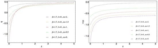
Figure 1.
Graphical behavior of the deceleration parameter q and of the varying ghost dark energy (DE), Equation (21), against redshift z. corresponds to the usual ghost DE.
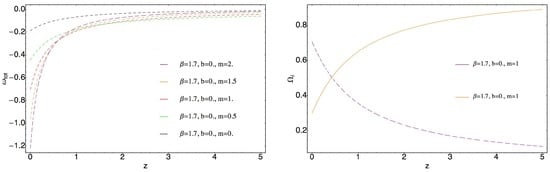
Figure 2.
Graphical behavior of EoS parameter of the effective fluid and against redshift z. Purple curve corresponds to , and the orange curve corresponds to . corresponds to the usual ghost DE. is defined according to Equation (23).
Table 3.
Present day values of , and q for various values of the parameter m, when , , while and . corresponds to the usual ghost DE.
2.1.2. Interacting Model
The energy density of DM in the case of interacting model according to Equations (18) and (22) reads as
In this case also the parameter m has significant effect on behavior of the deceleration parameter q and EoS parameter of the varying ghost DE given by Equation (Figure 3 of Reference [58]). In this model the best fit of the distance modulus to observational data is possible when , , , , , , , and the transition redshift is . This model is also free from CCP (see Figure 4 of Reference [58]) with . Bottom panels of Figures 3 and 4 of Reference [58] present graphical behavior of q, , and depending on the interaction parameter b for a fixed value of the parameter m. In Table 4 and Table 5 the present day values of the statefinder pair , and q parameters are presented. Comparison of theoretical results with observational data left only quintessence behavior for DE and the total effective fluid. Numerical analysis presented in Reference [58] directly indicates creation of massless particles in an appropriate radiation dominated expanding universe which evolving gives LSU (with suggested varying ghost DE) compatible with recent observational data. On the other hand, massless particles in these models (non-interacting and interacting) are not created immediately. Creation requires some time to start. Moreover, the total number of created massless particles for both models is an increasing function. Moreover, massless particle creation will adopt a periodic character in recent LSU.
Table 4.
Present day values of the statefinder pair , and q for various values of the parameter m, when , , while and . corresponds to the usual ghost DE. and .
Table 5.
Present day values of the statefinder pair , and q for various values of the interaction parameter b, when , , while and . and .
2.2. Cosmological Model with
In this subsection one will present the results corresponding to a model of the low redshift universe with another model of the varying ghost DE having the following energy density [59]
where α, β and m are constants and is the energy density of the pressureless DM. Such consideration is an attempt to have better understanding of the seeds for DE formation in early universe due to existence of DM. It is easy to see that Equations (25) and (17) with Equation (22) allows us to obtain EoS parameter of the varying ghost DE in terms of and as
where , and . To obtain Equation (26) and that
where
is taken into account. On the other hand, for this model the deceleration parameter reads as
The study presented in Reference [59] indicates that the decrease of m leads to increase of transition redshift and to decrease of the present day values of the deceleration parameter q and . Moreover, the increase of b leads to increase the transition redshift and to decrease of the present day values of and q. Moreover, in low redshift universe parameter b has a significant impact on these parameters. , and , , , , and constraints on the model parameters have been obtained during the comparison of the modulus distance with observational data to have the best fit. Present day values of the statefinder pair , and q are presented in Table 6. Graphical behavior of and against redshift z is presented in Figure 2 of Reference [59].
Table 6.
Present day values of , , q and appropriate redshift transition for the various values of the parameter m, when , and , , , and . corresponds to the usual ghost DE.
Statefinder Hierarchy and Thermodynamics
It is easy to see, that if one starts from the first law of thermodynamics
and with an assumption that DE, DM, radiation and event horizon are in thermal equilibrium, after some mathematics for for the varying ghost DE, Equation (25), one obtains [59]
where is given by Equation (26) and the case , corresponds to thermodynamics of the non-interacting varying ghost DE model. Moreover, the graphical behavior of according to Equation (A11) against redshift z presented in Reference [59] indicates that in statefinder hierarchy is a good indicator for this model. Moreover, it gives clear indication about possible deviation from ΛCDM model. The cosmographic analysis demonstrated that suggested cosmological model is a good model for low redshift universe. Moreover, this is a model with radiation like effective fluid for high redshift, which evolves to a quintessence DE in present universe. Another interesting result of Reference [59] is the demonstration of massless particle creation in a radiation dominated universe (see Figure 4 of Reference [59]).
2.3. Cosmological Model with
In Section 2.1 and Section 2.2 the subject of study was accelerated expansion of LSU, where a varying ghost DE of a certain type can take the role of DE. The model of the varying ghost DE with
presented in Reference [60] is another phenomenological modification of the ghost DE and completes the logical chain of considered modifications. It is obvious α, m and β should accepts appropriate values to have . One sees that the power law function of the energy density of the DM is considered. The ghost DE model, Equation (32), may also be understood as an example of a fluid introduced in References [43,44]. The first model considered in Reference [60] is a cosmological scenario where DE and DM do not interact. One starts with the presentation of the results corresponding to this scenario taking into account the constraints which were obtained Reference [60] according to the best fit of theoretical results to luminosity distance.
2.3.1. Non-Interacting Model
In the case of suggested modification in non-interacting model the EoS of the varying ghost DE has the following form
with , while in the case , . On the other hand, the deceleration parameter q of this model accepts the following form
Despite , for the deceleration parameter q one have
while for
Demand discussed in Reference [60] on , and for simplicity , gives the following constraints on and m
The study of Reference [60] provides a self-consistent picture about the behavior of the deceleration parameter, EoS parameter of the varying ghost DE and EoS of the effective fluid for low and high redshift. In particular, the attention of the authors has been concentrated on the study of the impact of m parameter on the behavior and present day values of mentioned cosmological parameters. It has been found that correct dynamics of , and provides a phase transition from a decelerated expanding universe to recent accelerated expanding universe and with an increase of m the transition redshift will decrease. For the reconstruction of thermodynamics of DE model one should start from the first law of thermodynamics and after some trivial mathematics for the dynamics of the entropy will be obtained
On the other hand, in Reference [60] the forms of two parameters of statefinder analysis are presented corresponding to this case.
2.3.2. Interacting Model with
The consideration of interaction term given by Equation (22), gives EoS parameter and the deceleration parameter q of the model as follows
As it is pointed in Reference [60], for , , but q is finite and is equal to
and case should be excluded, since with , and q tend to infinity. It is easy to see that the dynamics of the entropy of the varying ghost DE reads as
where
and
The graphical behavior of cosmological parameters and the present day values of these parameters summarized in Reference [60] directly indicate viability of considered model according to observational data.
2.3.3. Interacting Model with
Another model considered in Reference [60] assumes that the non-gravitational interaction is sign changeable and reads as
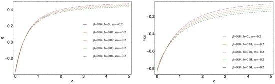
In Figure 3 the redshift dependent behavior of the deceleration parameter q and EoS parameter of the varying ghost DE, Equation (32), corresponding to different values of the parameter b for fixed values of β and m are plotted. It can be seen, that the considered sign changeable interaction, Equation (46), leaves unaffected the transition redshift and a distinguishing interacting models from non interacting is not possible. An estimation of the present day values of and for this model gives the same picture (for small values of b). The considered model is a model of a universe where
and the dynamics of the entropy of the varying ghost DE, Equation (32), has the following form
There is given by Equation (47). It is evident from Equation (48), that when , then , therefore in order to have LSU with accelerated expansion with , and for simplicity with , it is necessary, that
For universe with , i.e., matter dominated universe
2.3.4. Interacting Model with
Discussed sign changeable interaction, Equation (46), is only an option. The following formulation
provides another option and indicates that when DM will be transferred to DE, otherwise DE will be transferred to DM. If one considers the interaction, Equation (53), then in such universe, EoS parameter of the varying ghost DE has the following form [60]
and the deceleration parameter reads as [60]
where . In order to obtain LSU with accelerated expansion with , and for simplicity with , it is necessary [60]
The study of Reference [60] shows that one has the model with the correct behavior of cosmological parameters providing phase transition between decelerated and accelerated expansion of LSU. Moreover, in Reference [60] another model of interaction with also has been considered. The difference between these two models is the sign of the parameter b, therefore consideration of instead of b will describe physics of two models. Results related to these two models of the interaction are compared in Figures 7 and 8 of Reference [60]. For the dynamics of the entropy of the varying ghost DE considered in this subsection has the following form [60]
where is given by Equation (54), and interaction parameter b has been changed to . The study of Reference [60] shows also that parameter from the statefinder hierarchy is a good indicator to distinguish the models, therefore attention can be concentrated on it only. Moreover, the study of Reference [60] shows that is a good analysis for considered models. However, analysis is better for low redshif analysis.
3. Alternative Look at the Problem
The purpose of this section is to discuss various cosmological models applicable to accelerated expansion of LSU providing an alternative look to the problem. In particular, two models considered in this section belong to the class of the models where the dynamics of the background is still according to GR, however exotic forms of EoS and the interaction term between DE and DM is used. Instead of directly solving the field equations for these models, phase space analysis has been performed. It is known that in the phase space of a dynamical system all its possible states are represented making it very useful tool for modern cosmology. To analyse the dynamical system of the interacting polytropic gases considered in this section, one follows to existing scientific literature (see for instance [83]). There is a huge number of articles presenting the phase space analysis of different cosmological models [83,84,85,86,87,88,89,90] (to mention a few).
3.1. LSU with Interacting Polytropic Gas
Polytropic gas with non-linear EoS of the following
where K and n are two constants, has important applications in astrophysics and it is one of the models of dark fluids used in modern cosmology. In Reference [91] various cosmological scenarios with non-linear interacting polytropic gas models has been considered. Namely, two phenomenological possibilities for interaction term are considered: non-linear and sign changeable non-linear interactions. In particular, the following forms of interaction will be considered
and
ρ is the energy density either of the effective fluid or one of the components of the effective fluid. is the product of the energy densities of DE and DM.
3.1.1. Interacting Model with
The study of Reference [91] starts with the model, when the following interaction is considered
The autonomous system of this model reads as
It has been found, that only one physically reasonable stable critical point exists
when
or
Moreover, this solution is simply a late time scaling attractor, because
The study shows, that this late time scaling attractor describes the state of universe with , and EoS of the polytropic gas exhibits a phantom behavior (quintessence behavior is not possible) with
when
or
or
3.1.2. Interacting Model with
In the second model conidered in Reference [91] the following form for the interacting has been considered
The study shows that only one late time scaling attractor exists ()
obtained from the following autonomous system
For this model, it is not hard to see that , , while
and
Discussed late time scaling attractor represents a universe where the polytropic gas is phantom DE, when one of the following conditions take a place
or
3.1.3. Interacting Model with
The third model studied in Reference [91] is a cosmological model with the following form of interaction
having four critical points and only one is a physically reasonable and has the following form (E.1.3)
According to Reference [91] this solution is a late time scaling attractor describing universe with , ,
and
where the polytropic gas is phantom DE, when
or
3.1.4. Sign Changeable Interactions
On the other hand in Reference [91] an attempt has been forwarded to construct new forms of sign changeable interactions for the interaction terms considered in Section 3.1.1, Section 3.1.2 and Section 3.1.3. In particular, the deceleration parameter q has been involved. The result (critical points) of the study presented in Reference [91] is summarized in Table 7.
In particular, the forms for Q have been considered
and
Analysis show that obtained critical points are not stable. Compared with the interactions terms in Section 3.1.1, Section 3.1.2 and Section 3.1.3, appropriate sign changeable interactions do not allow to obtain late time attractors.
3.2. LSU with a Varying Polytropic Gas
In this section one will discuss results of the study presented in Reference [92]. The study of Reference [92] involves new idea/ phenomenological model of dark fluid constructed in analogue with a varying Chaplygin gas of the following form
In particular, in Reference [92] the following model of varying polytropic gas
where A, B, k and n are constants, is considered. In addition, pressureless DM to be the second component of recent low redshift universe is assumed to exist. Moreover, the forms of interactions considered in Reference [92] are particular examples obtained from
m, b and γ are constants. There the subscript i stands for the energy density either of effective fluid, or one of dark components. The study in Reference [92] starts form the models containing fixed sign interactions, which correspond to in Equation (92) with , , and . The lower limit on is due to PLANCK 2015 satellite experiment constraints [93].
3.2.1. Interaction
The first cosmological model studied in Reference [92] involves the following interaction
between varying polytropic DE, Equation (91), and CDM. The autonomous system of this model reads as [92]
and admits only one physically reasonable stable critical point (is either a stable node or stable focus) of the following form
It is easy to see, that straightforward calculations give
indicating that a solution of CCP directly depends on parameter b of interaction Equation (93). describes the universe where , and EoS parameter of the varying polytropic DE reads as
In case of considered constraints in Reference [92] one will have only phantom polytropic dark fluid. The study of Reference [92] reveals possible phase transition to accelerated expending low redshift universe. On the other hand, the study of this model has been completed by estimation of the present day values of and statefinder parameters , which are summarized in Table 8 of this work.
Table 8.
Present day values of and statefinder parameters for the cosmological model where , and , while the interaction is given by Equation (93).
3.2.2. Interaction
The second cosmological model considered in Reference [92] admits the following form of the interaction
giving two late time attractors (Table 9). However, an attractor with and , can not describe accelerated expansion of recent LSU, therefore it is out of the future discussion. Late time attractor with and describes the state of low redshift universe with , and i.e it describes de Sitter universe (according to the constraints considered in Reference [92]). On the other hand in Table 10 present day values of and statefinder parameters are summarized and the study revealed possible phase transition to accelerated expending low redshift universe.
Table 10.
Present day values of and statefinder parameters for the cosmological model where , and , while the interaction is given via Equation (99). The values of the parameters are due to the behavior of the cosmological parameters presented in Figure 2 of Reference [92]. .
3.2.3. Interaction
Another possibility studied in Reference [92] is cosmological model where the interaction between dark components reads as
with only one late time attractor (C.3.1 with ) of the following form
, and
giving a phantom LSU when . On the other hand, when polytropic dark fluid is a CC with . In Reference [92] the graphical behavior of the cosmological parameters reveals the phase transition between decelerated and accelerated expansion.
3.2.4. Interaction
In addition to considered three forms of interactions, in Reference [92] some forms of sign changeable interactions also has been discussed to complete the study. In particular the following form of sign changeable interaction
has been considered and demonstrated, that only one critical point exists (E.4.1 which is either stable node or stable focus) with
, and . On the other hand, for this model is equal to and in Reference [92] was assumed, which directly indicates that is physically reasonable only with . Therefore, according to Reference [92] describes a state of LSU, where only varying polytropic dark energy given by Equation (91) will dominate (an example of de Sitter universe). Moreover, the considered model has phase transition to an accelerated expanding low redshift universe.
If interaction of the following form is considered
between varying polytropic DE and DM, then only one late time attractor will exist for this model, which is an example de Sitter universe admitting phase transition (see Reference [92]).
3.2.5. Interaction
Autonomous system of cosmological model where interaction between suggested DE and DM has the following form (the last model considered in Reference [92])
has one critical point (C.6.1)
and describe a model of universe with , and
However, in this case is a physically reasonable solution if (according to considered constrains), describing de Sitter universe. Moreover, it is easy to see that the explicit forms of the trace
and the determinant
of the appropriate Jacobian matrix indicate for attractor to be either stable node or stable focus. Present day values of and statefinder parameters , for different values of the parameters of all models studied in Reference [92] are summarized in appropriate tables (for more details on this issue one referees the readers to Reference [92]).
3.3. Cosmological Models with Generalized Holographic DE
In this subsection, following Reference [94], one will consider particular model of the generalized holographic DE with the Nojiri- Odintsov cut-off defined as [24].
with
where it is the future horizon and defined as
while c, , and are numerical constants.
3.3.1. Models with
Generalized holographic DE model of Reference [24] includes arbitrary cut-off depending on , scale factor, H etc and their derivatives. In Reference [94] particular class of such generalized holographic DE model with Nojiri-Odintsov cut-off as Equation (112) has been considered. The cosmological model of LSU, where the interaction between the dark energy and dark matter is given by contains the DE with the following EoS parameter
while the deceleration parameter q reads as
Analysis of Reference [94] shows that in such model (transition redshift) when and the present day value of q defined by Equation (115) will decrease, the transition redshift will increase, when the value of the interaction parameter b will increase. Moreover, an increase of the interaction parameter b will speed up an increase of the amount of and this model is free from CCP. Moreover, the study of Reference [94] indicates clearly, that the impact of the interaction is imprinted into the dynamics of and . Moreover, for the value of the EoS parameter of DE (recent epoch) satisfies to the constraints according to the Planck satellite 2015 experiments. On the other hand, in this case with an increase of b the EoS will change its nature from quintessence to phantom (for higher redshifts), while for the lower redshifts gives an increase of and a decrease of . Another constraint on the parameter b is due to the demand for DE to have only the quintessence nature. From Table 11 one sees that an increase of b will decrease and increase the present day values of r and s parameters, respectively.
Table 11.
Present day values of the deceleration parameter q, of interacting dark energy, statefinder parameters and the value of the transition redshift for several values of the interaction parameter b, when the interaction is given by . The best fit of the theoretical results to the recent observational data has been obtained for , , , .
3.3.2. Models with Non-Linear Interactions
The cosmographic study of Reference [94] has been completed with an assumption about possible existence of the interaction between DE and DM of the following form
Straightforward calculations showed that such assumption gives a universe, where the EoS parameter of DE and the deceleration parameter read as
and
The appropriate comparison of the results for the cosmological models where the interaction is given by , Equation (116),
and
is presented in Reference [94]. The analysis shows, that with the interaction one will obtain the highest value for the transition redshift , while Equations (116), (119) and (120) interactions will increase . Moreover the study shoes that the maximum and minimal present day values for the deceleration parameter will be obtained in case of and , respectively. It also has been found that the significantly will be affected in case of and the dynamics of and carry information about the nature of the interactions. Moreover, the author of Reference [94] demonstrated, that with and Equation (120) DE is phantom, while in case of and when the interaction terms are given by Equations (116) and (119), DE is quintessence (for higher redshifts). However, during the evolution DE will change the nature giving either a quintessence universe, or a phantom universe. Such behavior has been found directly imprinted on the behavior of the other parameters.
Besides cosmographic analysis, the models have been studied by and analysis and the graphical behavior (redshift dependent) of the and parametes are presented in Figure 4 and Figure 5, respectively. Figures demonstrate departures from ΛCDM model ( line). Moreover, one can see clearly, that analysis is good enough for these models, while analysis shows that at lower redshifts non-gravitational interaction can be switched off. On the other hand parameter (corresponding to the statefinder hierarchy analysis) is good to study the models for lower redshifts only (Figure 6). In Reference [94] the validity of the generalized second law of thermodynamics
with it is the entropy associated with the horizon, has been confirmed. On the other hand, has been obtained from the validity of the generalized second law of thermodynamics. One can see that in this case the DE will have phantom nature at higher redshifts.
Figure 4.
Graphical behavior of the parameter against the redshift z. The blue curve represents non interacting model with , the orange curve represents the model, when the interaction is given by , the red curve represents the model when the interaction is given by Equation (116), the green curve represents the model with the interaction given by Equation (119), while the black curve represents the model with the interaction given by Equation (120), when , , , . The left plot corresponds to the case when . The right plot represents the case when for the interacting models .
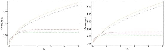
Figure 5.
Graphical behavior of the parameters against the redshift z. The blue curve represents non interacting model with , the orange curve represents the model, when the interaction is given by , the red curve represents the model when the interaction is given by Equation (116), the green curve represents the model with the interaction given by Equation (119), while the black curve represents the model with the interaction given by Equation (120), when , , , . The left plot corresponds to the case when . The right plot represents the case when for the interacting models . and .
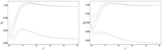
Figure 6.
Graphical behavior of the parameters against the redshift z. The blue curve represents non interacting model with , the orange curve represents the model, when the interaction is given by , the red curve represents the model when the interaction is given by Equation (116), the green curve represents the model with the interaction given by Equation (119), while the black curve represents the model with the interaction given by Equation (120), when , , , . The left plot corresponds to the case when . The right plot represents the case when for the interacting models .
4. Conclusions
Accelerated expansion of LSU is one of the long standing problems. There are various attempts to solve this problem and in this review paper one has presented some of the possible new solutions of this problem. In particular, it has been demonstrated, that the problem of accelerated expansion can be solved by the new models of the varying ghost DE. Moreover, for two models massless particle creation in appropriate readiation dominated universe has been observed numerically. On the other hand within phase space analysis two alternative possibilities have been demonstrated. In the first case new models of nonlinear and nonlinear sing changeable interactions have been considered between polytropic DE and CDM. On the other hand for the second case, the solution to the problem has been demonstrated within new phenomenological modification of polytropic gas. Finally, the third alternative possibility presented in this work is due to the generalized holographic DE model with a specific form of cut-off. In this case, various forms of non-gravitational interaction between DE and DM have been considered to complete the study. Presented all models either are free from CPP, or the CCP can be avoided due to appropriate interaction. All models give phase transition between decelerated and accelerated expansion.
Comparison of the results with observational data proved the viability of suggested scenarios. On the other hand, one should try to deepen the position of these models involving into the game other forms of non-gravitational interaction, find scalar field description of the models (find the form of the potential) and construct, for instance, the theory. There is another important direction of research related to the classification and understanding of the formation of finite time singularities in these models [95,96,97,98,99,100]. One hopes that results of this study will be reported soon elsewhere.
Acknowledgments
We thank referees for helpful comments and suggestions.
Conflicts of Interest
The author declares no conflicts of interest.
Appendix A
The last decade has been fruitful for the research on problems of universe and allowed to collect a huge amount of observational/scientific data. Such success is directly related to the new and innovative developments in technology. Available sets of observational data allow to use various tests to compare the theoretical results and obtain appropriate constraints on the parameters of the models. The first attempt to constraint the parameters of the model could be provided from data. For this case the test requires to minimize defined as
where it is the theoretical value of the Hubble parameter H obtained from the Friedmann equation for a given redshift , while represents appropriate estimates of the Hubble parameter from various missions with its error . The goal of this test is to obtain constraints on the parameters of the model via minimizing the . Appropriate constraints can be obtained using data from Supernova Cosmology project through the fitting the distance modulus ,
where , with absolute magnitude of the SNeIa and h being the Hubble parameter at present in units of with
and the to fit the data is then given by
In this case the values of the parameters minimizing must be computed. One can use also data from CMB and BAO to obtain appropriate constraints. Moreover, tests can be applied simultaneously and the demand in this case is to minimize the value of the total
where . Additionally, one can impose constraints on phenomenological models using, for instance, observational data corresponding to the active galactic nucleus clustering. There is also an active discussion on possible constraints provided by strong and weak gravitational lensing data if one has a good knowledge of lens models. The fact that the cosmological gravitational field bends the paths of the light rays when they pass through the astronomical objects one can extract important information, for instance, on the mass distribution. Therefore. gravitational lensing has developed into an important astrophysical tool for probing the cosmology, the structure formation and the evolution of galaxies. Data fitting and the estimation of the parameters of the cosmological model in case of strong gravitational lensing is based on the distance ratio
where and are the redshifts of the source and lens, respectively, while
it is the angular diameter distance between and in a flat universe (in units of ). It is obvious, that the angular diameter distance carries all information concerning to the background dynamics of universe, therefore data fitting test like
also can be used to obtain appropriate constraints. Consideration of allows one to eliminate uncertainty between the stellar velocity dispersion and the velocity dispersion of the singular isothermal sphere/ellipsoid [101,102,103,104] (and references therein which can provide additional references to dark energy models, interaction in modern cosmology, modified theories of gravity, etc.). One can involve various geometrical tools like statefinder analysis with and parameters, , , and statefinder hierarchy analysis to study cosmological models. For instance, analysis suggests to study the behavior of the DE in and plane, where is the derivative of EoS of DE with respect to . On the other hand, the three-point diagnostic
where the two point reads as
is also very convenient tool as well. An interesting approach to study DE models is statefinder hierarchy analysis requiring to study the following parameters
etc. reads as
with
References
- Riess, A.G.; Filippenko, A.V.; Challis, P.; Clocchiatti, A.; Diercks, A.; Garnavich, P.M.; Gilliland, R.L.; Hogan, C.J.; Jha, S.; Kirshner, R.P.; et al. Observational evidence from supernovae for an accelerating universe and a cosmological constant. Astron. J. 1998, 116, 1009–1038. [Google Scholar] [CrossRef]
- Perlmutter, S.; Aldering, G.; Goldhaber, G.; Knop, R.A.; Nugent, P.; Castro, P.G.; Deustua, S.; Fabbro, S.; Goobar, A.; Groom, D.E.; et al. Measurements of Ω and Λ from 42 high-redshift supernovae. Astrophys. J. 1999, 517, 565–586. [Google Scholar] [CrossRef]
- Tegmark, M.; Strauss, M.; Blanton, M.; Abazajian, K.; Dodelson, S.; Sandvik, H.; Wang, X.; Weinberg, D.; Zehavi, I.; Bahcall, N.; et al. Cosmological parameters from SDSS and WMAP. Phys. Rev. D 2004, 69, 103501. [Google Scholar] [CrossRef]
- Hawkins, E.; Maddox, S.; Cole, S.; Lahav, O.; Madgwick, D.; Norberg, P.; Peacock, J.; Baldry, I.; Baugh, C.; Bland-Hawthorn, J.; et al. The 2dF Galaxy Redshift Survey: Correlation functions, peculiar velocities and the matter density of the universe. Mon. Not. Roy. Astron. Soc. 2003, 346, 78–96. [Google Scholar] [CrossRef]
- Yoo, J.; Watanabe, Y. Theoretical Models of Dark Energy. Int. J. Mod. Phys. D 2012, 21, 1230002. [Google Scholar] [CrossRef]
- Balakin, A.B. Electrodynamics of a Cosmic Dark Fluid. Symmetry 2016, 8, 56. [Google Scholar] [CrossRef]
- Bradav, M.; Allen, S.W.; Treu, T.; Ebeling, H.; Massey, R.; Morris, R.G.; von der Linden, A.; Applegate, D. Revealing the Properties of Dark Matter in the Merging Cluster MACS J0025.4–1222*. Astrophys. J. 2008, 687, 959–967. [Google Scholar] [CrossRef]
- Bosma, A. 21-cm line studies of spiral galaxies. II. The distribution and kinematics of neutral hydrogen in spiral galaxies of various morphological types. Astron. J. 1981, 86, 1825–1846. [Google Scholar] [CrossRef]
- Liddle, A. An introduction to cosmological inflation. arXiv, 1999; arXiv:astro-ph/9901124. [Google Scholar]
- Andrei, L. Inflationary Cosmology after Planck 2013. arXiv, 2013; arXiv:1402.0526. [Google Scholar]
- Guth, H.; Kaiser, D.I.; Nomura, Y. Inflationary paradigm after Planck 2013. Phys. Lett. B 2014, 733, 112–119. [Google Scholar] [CrossRef]
- Bamba, K.; Odintsov, S.D. Inflationary cosmology in modified gravity theories. Symmetry 2015, 7, 220–240. [Google Scholar] [CrossRef]
- Nojiri, S.; Odintsov, S.D. Unified cosmic history in modified gravity: From F (R) theory to Lorentz non-invariant models. Phys. Rep. 2011, 505, 59–144. [Google Scholar] [CrossRef]
- Capozziello, S.; Nojiri, S.; Odintsov, S.D. Unified phantom cosmology: Inflation, dark energy and dark matter under the same standard. Phys. Lett. B 2006, 632, 597–604. [Google Scholar] [CrossRef]
- Velten, H.E.S.; vom Marttens, R.F.; Zimdahl, W. Aspects of the cosmological “coincidence problem”. Eur. Phys. J. C 2014, 74, 3160. [Google Scholar] [CrossRef]
- Sivanandam, N. Is the Cosmological Coincidence a Problem? Phys. Rev. D 2013, 87, 083514. [Google Scholar] [CrossRef]
- Martin, J. Everything you always wanted to know about the cosmological constant problem (but were afraid to ask). Comptes Rendus Phys. 2012, 13, 566–665. [Google Scholar] [CrossRef]
- Bamba, K.; Capozziello, S.; Nojiri, S.; Odintsov, S.D. Dark energy cosmology: The equivalent description via different theoretical models and cosmography tests. Astrophys. Space Sci. 2012, 342, 155–228. [Google Scholar] [CrossRef]
- Nojiri, S.; Odintsov, S.D. Is the future universe singular: Dark Matter versus modified gravity? Phys. Lett. B 2010, 686, 44–48. [Google Scholar] [CrossRef]
- Garcia-Salcedo, R.; Gonzalez, T.; Quiros, I. No compelling cosmological models come out of magnetic universes which are based on nonlinear electrodynamics. Phys. Rev. D 2014, 89, 084047. [Google Scholar] [CrossRef]
- Elizalde, E.; Nojiri, S.; Odintsov, S.D. Late-time cosmology in a (phantom) scalar-ensor theory: Dark energy and the cosmic speed-up. Phys. Rev. D 2004, 70, 043539. [Google Scholar] [CrossRef]
- Elizalde, E.; Nojiri, S.; Odintsov, S.D.; Saez-Gomez, D.; Faraoni, V. Reconstructing the universe history, from inflation to acceleration, with phantom and canonical scalar fields. Phys. Rev. D 2008, 77, 106005. [Google Scholar] [CrossRef]
- Nojiri, S.; Odintsov, S.D. Final state and thermodynamics of a dark energy universe. Phys. Rev. D 2004, 70, 103522. [Google Scholar] [CrossRef]
- Nojiri, S.; Odintsov, S.D. Unifying phantom inflation with late-time acceleration: Scalar phantom– non-phantom transition model and generalized holographic dark energy. Gen. Relativ. Gravit. 2006, 38, 1285–1304. [Google Scholar] [CrossRef]
- Nojiri, S.; Odintsov, S.D. Quantum deSitter cosmology and phantom matter. Phys. Lett. B 2003, 562, 147–152. [Google Scholar] [CrossRef]
- Nojiri, S.; Odintsov, S.D. The oscillating dark energy: future singularity and coincidence problem. Phys. Lett. B 2006, 637, 139–148. [Google Scholar] [CrossRef]
- Elizalde, E.; Makarenko, A. N.; Nojiri, S.; Obukhov, V.V.; Odintsov, S.D. Multiple Λ cosmology with string landscape features and future singularities. Astrophys. Space Sci. 2013, 344, 479–488. [Google Scholar] [CrossRef]
- Brevik, I.; Elizalde, E.; Nojiri, S.; Odintsov, S.D. Viscous little rip cosmology. Phys. Rev. D 2011, 84, 103508. [Google Scholar] [CrossRef]
- Brevik, I.; Myrzakulov, R.; Nojiri, S.; Odintsov, S.D. Turbulence and Little Rip Cosmology. Phys. Rev. D 2012, 86, 063007. [Google Scholar] [CrossRef]
- Astashenok, A.V.; Odintsov, S.D. Confronting dark energy models mimicking ΛCDM epoch with observational constraints: Future cosmological perturbations decay or future Rip? Phys. Lett. B 2013, 718, 1194–1202. [Google Scholar] [CrossRef]
- Astashenok, A.V.; Nojiri, S.; Odintsov, S.D.; Scherrer, R.J. Scalar dark energy models mimicking ΛCDM with arbitrary future evolution. Phys. Lett. B 2012, 713, 145–153. [Google Scholar] [CrossRef]
- Kahya, E.O.; Khurshudyan, M.; Pourhassan, B.; Myrzakulov, R.; Pasqua, A. Higher order corrections of the extended Chaplygin gas cosmology with varying G and λ. Eur. Phys. J. C 2015, 75, 43. [Google Scholar] [CrossRef]
- Guo, Z.K.; Ohta, N. Parametrizations of the dark energy density energy and scalar potential. Mod. Phys. Lett. A 2007, 22, 883–890. [Google Scholar] [CrossRef]
- Dutta, S.; Saridakis, E.N.; Scherrer, R.J. Dark energy from a quintessence (phantom) field rolling near a potential minimum (maximum). Phys. Rev. D 2009, 79, 103005. [Google Scholar] [CrossRef]
- Saridakis, E.N.; Sushkov, S.V. Quintessence and phantom cosmology with nonminimal derivative coupling. Phys. Rev. D 2010, 81, 083510. [Google Scholar] [CrossRef]
- Sadeghi, J.; Khurshudyan, M.; Hakobyan, M.; Farahani, H. Phenomenological Fluids from Interacting Tachyonic Scalar Fields. Int. J. Theor. Phys. 2014, 53, 2246–2260. [Google Scholar] [CrossRef]
- Brevik, I.; Gorbunova, O.; Nojiri, S.; Odintsov, S.D. On Isotropic Turbulence in the Dark Fluid Universe. Eur. Phys. J. C 2011, 71, 1629. [Google Scholar] [CrossRef]
- Khurshudyan, M.; Myrzakulov, R. Phase space analysis of some interacting Chaplygin gas models. arXiv, 2015; arXiv:1509.02263. [Google Scholar]
- Pourhassan, B.; Kahya, E.O. Extended Chaplygin gas model. Results Phys. 2004, 4, 101102. [Google Scholar] [CrossRef]
- Kahya, E.O.; Pourhassan, B. The universe dominated by the extended Chaplygin gas. Mod. Phys. Lett. A 2015, 30, 1550070. [Google Scholar] [CrossRef]
- Khurshudyan, M.; Chubaryan, E.; Pourhassan, B. Interacting Quintessence Models of Dark Energy. Int. J. Theor. Phys. 2014, 53, 2370–2378. [Google Scholar] [CrossRef]
- Capozziello, S.; Cardone, V.F.; Elizalde, E.; Nojiri, S.; Odintsov, S.D. Observational constraints on dark energy with generalized equations of state. Phys. Rev. D 2006, 73, 043512. [Google Scholar] [CrossRef]
- Nojiri, S.; Odintsov, S.D. Inhomogeneous equation of state of the universe: Phantom era, future singularity, and crossing the phantom barrier. Phys. Rev. D 2005, 72, 023003. [Google Scholar] [CrossRef]
- Cardone, V.F.; Troisi, A.; Capozziello, S. Inflessence: A Phenomenological model for inflationary quintessence. Phys. Rev. D 2006, 73, 043512. [Google Scholar]
- Ferreira, P.G.; Joyce, M. Structure Formation with a Self-Tuning Scalar Field. Phys. Rev. Lett. 1997, 79, 4740–4743. [Google Scholar]
- Copeland, E.J.; Sami, M.; Tsujikawa, S. Dynamics of dark energy. Int. J. Mod. Phys. D 2006, 15, 1753–1936. [Google Scholar] [CrossRef]
- Copeland, E.J.; Liddle, A.R.; Wands, D. Exponential potentials and cosmological scaling solutions. Phys. Rev. D 1998, 57, 4686–4690. [Google Scholar] [CrossRef]
- Gong, Y.G.; Wang, A.; Zhang, Y.-Z. Exact scaling solutions and fixed points for general scalar field. Phys. Lett. B 2006, 636, 286–292. [Google Scholar] [CrossRef]
- Bolotin, Y.L.; Kostenko, A.; Lemets, O.A.; Yerokhin, D.A. Cosmological Evolution With Interaction Between Dark Energy And Dark Matter. Int. J. Mod. Phys. D 2015, 24, 1530007. [Google Scholar] [CrossRef]
- Nojiri, S.; Odintsov, S.D. Introduction to Modified Gravity and Gravitational Alternative for Dark Energy. Int. J. Geom. Methods. Mod. Phys. 2007, 4, 115–146. [Google Scholar] [CrossRef]
- Clifton, T.; Ferreira, P.G.; Padilla, A.; Skordis, C. Modified Gravity and Cosmology. Phys. Rep. 2012, 513, 1–189. [Google Scholar] [CrossRef]
- Sahni, V.; Saini, T.D.; Starobinsky, A.A.; Alam, U. Statefinder—A new geometrical diagnostic of dark energy. JETP Lett. 2003, 77, 201–206. [Google Scholar] [CrossRef]
- Sahni, V.; Shafieloo, A.; Starobinsky, A.A. Two new diagnostics of dark energy. Phys. Rev. D 2008, 78, 103502. [Google Scholar] [CrossRef]
- Caldwell, R.R.; Linder, E.V. Limits of Quintessence. Phys. Rev. Lett. 2005, 95, 141301. [Google Scholar] [CrossRef] [PubMed]
- Arabsalmani, M.; Sahni, V. Statefinder hierarchy: An extended null diagnostic for concordance cosmology. Phys. Rev. D 2011, 83, 043501. [Google Scholar] [CrossRef]
- Sahni, V.; Shafieloo, A.; Starobinsky, A.A. Model-independent evidence for dark energy evolution from baryon acoustic oscillations. Astrophys. J. 2014, 793, L40. [Google Scholar] [CrossRef]
- Khurshudyan, M.; Khurshudyan, A.; Myrzakulov, R. Interacting varying ghost dark energy models in general relativity. Astrophys. Space Sci. 2015, 357, 113. [Google Scholar] [CrossRef]
- Khurshudyan, M. Low redshift universe and a varying ghost dark energy. Mod. Phys. Lett. A 2016, 31, 1650055. [Google Scholar] [CrossRef]
- Khurshudyan, M. Varying ghost dark energy and particle creation. Eur. Phys. J. Plus 2016, 131, 25. [Google Scholar] [CrossRef]
- Khurshudyan, M.Z.; Makarenko, A.N. On a phenomenology of the accelerated expansion with a varying ghost dark energy. Astrophys. Space Sci. 2016, 361, 187. [Google Scholar] [CrossRef]
- Zeldovich, Y.B. Simulated light scattering induced by absorption. JETP Lett. 1970, 12, 307. [Google Scholar] [CrossRef]
- Barrow, J.D. The deflationary universe: An instability of the de Sitter universe. Phys. Lett. B 1986, 180, 335–339. [Google Scholar] [CrossRef]
- Morikawa, M.; Sasaki, M. Entropy production in an expanding universe. Phys. Lett. B 1985, 165, 59–62. [Google Scholar] [CrossRef]
- Padmanabhan, T.; Chitre, S.M. Viscous universes. Phys. Lett. A 1987, 120, 433–436. [Google Scholar] [CrossRef]
- Zimdahl, W.; Pavon, D. Fluid cosmology with decay and production of particles. Gen. Relativ. Gravit. 1994, 26, 1259–1265. [Google Scholar] [CrossRef]
- Zimdahl, W.; Schwarz, D.J.; Balakin, A.B.; Pavon, D. Cosmic anti-friction and accelerated expansion. Phys. Rev. D 2001, 64, 063501. [Google Scholar] [CrossRef]
- Abramo, L.R.W.; Lima, J.A.S. Inflationary models driven by adiabatic matter creation. Class. Quantum Grav. 1996, 13, 2953–2964. [Google Scholar] [CrossRef]
- Gariel, J.; le Denmat, G. Matter creation and bulk viscosity in early cosmology. Phys. Lett. A 1995, 200, 11–16. [Google Scholar] [CrossRef]
- Lima, J.A.S.; Germano, A.S.M.; Abramo, L.R.W. FRW-type cosmologies with adiabatic matter creation. Phys. Rev. D 1996, 53, 4287. [Google Scholar] [CrossRef]
- Parker, L. Particle Creation in Expanding Universes. Phys. Rev. Lett. 1968, 21, 562. [Google Scholar] [CrossRef]
- Parker, L. Quantized Fields and Particle Creation in Expanding Universes. I. Phys. Rev. 1969, 183, 1057. [Google Scholar] [CrossRef]
- Parker, L. Quantized Fields and Particle Creation in Expanding Universes. II. Phys. Rev. D 1971, 3, 346. [Google Scholar] [CrossRef]
- Parker, L. Particle Creation in Isotropic Cosmologies. Phys. Rev. Lett. 1972, 28, 705. [Google Scholar] [CrossRef]
- Parker, L. Conformal Energy-Momentum Tensor in Riemannian Space-Time. Phys. Rev. D 1973, 7, 976. [Google Scholar] [CrossRef]
- Grib, A.A.; Pavlov, Y.V. Superheavy particles and the dark matter problem. Gravit. Cosmol. 2006, 12, 159–162. [Google Scholar]
- Grishchuk, L.P. Quantum effects in cosmology. Class. Quantum Grav. 1993, 10, 2449–2478. [Google Scholar] [CrossRef]
- Maia, M.R.G. Spectrum and energy density of relic gravitons in flat Robertson-Walker universes. Phys. Rev. D 1993, 48, 647–662. [Google Scholar] [CrossRef]
- Maia, M.R.G.; Barrow, J.D. Cosmological graviton production in general relativity and related gravity theories. Phys. Rev. D 1994, 50, 6262–6296. [Google Scholar] [CrossRef]
- Maia, M.R.G.; Lima, J.A.S. Graviton production in elliptical and hyperbolic universes. Phys. Rev. D 1996, 54, 6111–6121. [Google Scholar] [CrossRef]
- Pereira, S.H.; Bessab, C.H.G.; Lima, J.A.S. Quantized fields and gravitational particle creation in f (R) expanding universes. Phys. Lett. B 2010, 690, 103–107. [Google Scholar] [CrossRef]
- Pereira, S.H.; Aguilar, J.C.Z.; Romao, E.C. Massless particle creation in a f (R) expanding universe. arXiv, 2013; arXiv:1108.3346. [Google Scholar]
- Pereira, S.H.; Holanda, R.F.L. Particle creation in a f (R) theory with cosmological constraints. Gen. Relativ. Gravit. 2014, 46, 1699. [Google Scholar] [CrossRef]
- Xu, Y.D.; Huang, Z.G. The sign-changeable interaction between variable generalized Chaplygin gas and dark matter. Astrophys. Space Sci. 2013, 343, 807–811. [Google Scholar]
- Jarv, L.; Mohaupt, T.; Saueressig, F. Phase Space Analysis of Quintessence Cosmologies with a Double Exponential Potential. J. Cosmol. Astropart. Phys. 2004, 0408, 16. [Google Scholar] [CrossRef]
- Leon, G.; Saridakis, E.N. Phase-space analysis of Horava-Lifshitz cosmology. J. Cosmol. Astropart. Phys. 2009, 0911, 6. [Google Scholar] [CrossRef] [PubMed]
- Leon, G.; Saridakis, E.N. Dynamical analysis of generalized Galileon cosmology. J. Cosmol. Astropart. Phys. 2013, 1303, 025. [Google Scholar] [CrossRef]
- Leon, G.; Saavedra, J.; Saridakis, E.N. Cosmological behavior in extended nonlinear massive gravity. Class. Quantum Grav. 2013, 30, 135001. [Google Scholar] [CrossRef]
- Fadragas, C.R.; Leon, G.; Saridakis, E.N. Dynamical analysis of anisotropic scalar-field cosmologies for a wide range of potentials. Class. Quantum Grav. 2014, 31, 075018. [Google Scholar] [CrossRef]
- Xu, C.; Saridakis, E.N.; Leon, G. Phase-space analysis of teleparallel dark energy. J. Cosmol. Astropart. Phys. 2012, 07, 005. [Google Scholar] [CrossRef] [PubMed]
- Chen, X.; Gong, Y.; Saridakis, E.N. Phase-space analysis of interacting phantom cosmology. J. Cosmol. Astropart. Phys. 2009, 0904. [Google Scholar] [CrossRef]
- Khurshudyan, M. Some non linear interactions in polytropic gas cosmology: Phase space analysis. Astrophys. Space Sci. 2015, 360, 33. [Google Scholar] [CrossRef]
- Khurshudyan, M. A varying polytropic gas universe and phase space analysis. Mod. Phys. Lett. A 2016, 31, 1650097. [Google Scholar] [CrossRef]
- Ade, P.A.R.; Aghanim, N.; Arnaud, M.; Ashdown, M.; Aumont, J.; Baccigalupi, C.; Banday, A.J.; Barreiro, R.B.; Bartlett, J.G.; Bartolo, N.; et al. Planck 2015 results. XIII. Cosmological parameters. Astron. Astrophys. 2016, 594, A13. [Google Scholar] [CrossRef]
- Khurshudyan, M. On a holographic dark energy model with a Nojiri-Odintsov cut-off in general relativity. Astrophys. Space Sci. 2016, 361, 232. [Google Scholar] [CrossRef]
- Nojiri, S.; Odintsov, S.D.; Tsujikawa, S. Properties of singularities in (phantom) dark energy universe. Phys. Rev. D 2015, 71, 063004. [Google Scholar] [CrossRef]
- Nojiri, S.; Odintsov, S.D.; Oikonomou, V.K. A quantitative analysis of singular inflation with scalar-tensor and modified gravity. Phys. Rev. D 2015, 91, 084059. [Google Scholar] [CrossRef]
- Odintsov, S.D.; Oikonomou, V.K. Inflation in exponential scalar model and finite-time singularity induced instability. arXiv, 2015; arXiv:1507.05273. [Google Scholar]
- Odintsov, S.D.; Oikonomou, V.K. Singular Inflationary Universe from F(R) Gravity. Phys. Rev. D 2015, 92, 124024. [Google Scholar] [CrossRef]
- Oikonomou, V.K. Singular Bouncing Cosmology from Gauss-Bonnet Modified Gravity. Phys. Rev. D 2015, 92, 124027. [Google Scholar] [CrossRef]
- Kleidis, K.; Oikonomou, V.K. Effects of Finite-time Singularities on Gravitational Waves. Astrophys. Space Sci. 2016, 361, 326. [Google Scholar] [CrossRef]
- Cid, A.; Labran, P. Observational constraints on a cosmological model with Lagrange multipliers. Phys. Lett. B 2012, 717, 10–16. [Google Scholar] [CrossRef]
- Farooq, M.O. Observational constraints on dark energy cosmological model parameters. arXiv, 2013; arXiv: 1309.3710. [Google Scholar]
- Cao, S.; Pan, Y.; Biesiada, M.; Godlowski, W.; Zhu, Z.-H. Constraints on cosmological models from strong gravitational lensing systems. J. Cosmol. Astropart. Phys. 2012, 3, 16. [Google Scholar] [CrossRef]
- Chen, Y.; Geng, C.-Q.; Cao, S.; Huang, Y.-M.; Zhu, Z.-H. Constraints on a CDM model from strong gravitational lensing and updated Hubble parameter measurements. J. Cosmol. Astropart. Phys. 2015, 2, 10. [Google Scholar] [CrossRef]
© 2016 by the author; licensee MDPI, Basel, Switzerland. This article is an open access article distributed under the terms and conditions of the Creative Commons Attribution (CC-BY) license (http://creativecommons.org/licenses/by/4.0/).