Scalar on Function Absolute Relative Error Regression: Functional Time Series Case

Abstract

This paper introduces a novel estimator for the functional regression model with a scalar response variable D and a functional predictor $\mathcal{C}$ taking values in a semi-metric space. The proposed estimator is obtained by minimizing the Least Absolute Relative Error (LARE) loss, an asymmetric criterion that measures prediction errors relative to the magnitude of the response variable. The theoretical properties of the estimator are established in the functional time series case by deriving its asymptotic distribution. This result provides a fundamental basis for some statistical inferences, including the construction of confidence intervals and the development of hypothesis tests for the regression operator. Unlike the conventional least absolute deviation or least squares criteria, the absolute relative error criterion offers a scale-invariant measure of prediction accuracy, making it particularly suitable when the response variable exhibits substantial variability. By the relative absolute deviations, the proposed approach reduces the impact of extreme observations, improves robustness to heteroscedasticity and outliers. Thus, approach enhances prediction performance in functional time series. The practical relevance of the proposed methodology is highlighted through extensive simulation experiments and an application to a real-world dataset, proving its computational simplicity, stability and accuracy.

1. Introduction

The analysis of functional time series constitutes a primordial topic in functional statistics. Usually, conventional methods are typically developed under the least squares framework, this paper proposes a novel nonparametric smoother based on the Absolute Relative Error (ARE) criterion. Based on its scale-invariant, the proposed approach offers an alternative robust approach to the classical least squares criterion. Such approach limits the impact of outliers and the heteroscedasticity of the data. Thus, the Functional ARE estimator has the potential to improve estimation accuracy, predictive performance, particularly in the complex structures.

The general framework of nonparametric functional data analysis is well developed in the the past few decades. Since the pioneering work of [1], the field has attracted considerable attention and has grown into a rich and active area of research. For example, Ref. [2] established the $L^p$-norm convergence of the kernel estimator for functional regression. The leading term expansion of the corresponding $L^p$ error was derived in [3], whereas [4] proved the asymptotic normality of the estimator under strong mixing conditions. Beyond the classical kernel approach, important methodological advances have also been achieved through M-estimation and local linear smoothing; see, for example, [5,6,7] for comprehensive developments in these directions.

Motivated by these developments, this paper focuses on relative error regression (ReR), as alternative regression framework in which prediction accuracy is assessed through relative absolute deviations. Such a criterion is often more appropriate in applications where the response variable exhibits substantial variability or where proportional prediction errors are of primary interest. Relative error regression has found important applications in several fields, including medicine [8] and finance [9]. Nevertheless, its nonparametric development remains relatively limited. The first contributions in this direction were made by [10], who investigated estimation based on the relative squared error criterion within multiplicative regression models. Ref. [11] proposed a nonparametric local linear estimator under the same framework. More recently, these methodologies have been extended to dependent data settings, including quasi-associated time series [12].

In the context of functional statistics, nonparametric relative error regression was pioneered by [13], who established the strong consistency and asymptotic normality of the proposed estimator. This topic was extended to accommodate more complex data settings. In particular, Ref. [14] generalized the methodology to incomplete functional data. They established the almost complete consistency of the adapted estimator for truncated data. More recent advances and methodological developments can be found in [15,16].

It is worth emphasizing that all existing studies in the functional relative have focused on relative squared error criteria, which is sensitive to atypical observations and large prediction errors. To overcome these limitations, we propose a new nonparametric functional regression estimator based on the Absolute Relative Error (ARE) criterion. By replacing squared relative deviations with absolute relative deviations, the proposed approach provides more robust and scale invariant measure of prediction accuracy. This formulation reduces the influence of outliers and offers stable predictor in the presence of heteroscedasticity., while retaining the intuitive relative interpretation of prediction errors. These properties make the proposed estimator particularly attractive for applications where the response variable exhibits high variability. Thus, in functional data analysis, where observations are often noisy, densely sampled, and characterized by the local fluctuations and high variability the gain is very important.

From a theoretical point of view the ARE framework is more challenging than the LSRE model. The LSRE estimator admits an explicit representation via the ratio of conditional inverse moments which facilitates its theoretical analysis. Conversely, the LARE estimator does not possess such a explicit expression. Therefore, the asymptotic behavior of the LARE model cannot be established through direct analytical arguments and instead requires the development of a suitable Bahadur representation. Moreover, this implicit formulation leads to additional computational challenges, as the estimator requires local, data-driven optimization rather than the direct estimation of a fixed operator. However, despite these technical difficulties, we derive the asymptotic distribution of the proposed estimator under standard conditions commonly assumed in nonparametric functional statistics. These assumptions explore both the infinite-dimensional nature of the functional predictor and the dependence structure of the data.

The second important advantage of the proposed methodology is that it applies to a large class of regression models than the existing Least Squares Relative Error (LSRE)-approach. In contrast to the existing LSRE approach, which requires the response variable to be strictly positive, the proposed LARE criterion does not impose such a restriction. Consequently, the new predictor is applicable to a large class of functional regression models. This flexibility is particularly valuable in the analysis of functional time series, where the observations exhibit temporal dependence and often display complex dynamic features that are absent in the independent setting. Therefore, the proposed methodology extends naturally beyond independent functional data and provides a robust framework for modeling the dependent functional processes encountered in practice.

Finally, the practical relevance of the proposed methodology is demonstrated through comprehensive simulation studies and real-world functional time series applications. The simulation experiments examine the finite-sample behavior of the proposed estimator under diverse dependence structures and noise levels, whereas the real-data examples highlight its practical effectiveness. The empirical findings consistently indicate that the proposed LARE estimator provides greater robustness, improved estimation accuracy, and superior predictive performance compared with the existing LSRE-based methodology, especially in challenging settings characterized by temporal dependence, heteroscedasticity, and atypical observations.

The rest of the paper is organized as follows. In Section 2, we introduce the proposed estimation procedure. Section 4 establishes the regularity conditions and the asymptotic theory of the estimator. Section 5 investigates its finite sample performance through simulation experiments and a real-data application is given in Section 6. Concluding remarks are given in Section 7, whereas all technical proofs are presented in Appendix A.

2. Functional Time Series Analysis by Functional LARE-Regression

Data Sampling

Recall that the primary objective of functional time series analysis is to predict the future behavior of an underlying continuous-time stochastic process. This is achieved by representing the process as a sequence of dependent functional observations, obtained by partitioning its continuous trajectories into successive time intervals. Each interval is then viewed as a single functional observation, preserving the intrinsic continuity of the data. Such a representation makes it possible to exploit the information contained in the historical trajectories to accurately predict the future characteristics of the process. Indeed, let ${\left\{Q_t\right\}}_{t\in [0,b)}$ be a real-valued continuous-time stochastic process. From $\left\{Q_t\right\}$, we construct a sequence of dependent functional random variables ${\left\{C_i\right\}}_{i=1}^N$ by partitioning the continuous trajectory into consecutive intervals of equal length b, namely,

$$C_i\left(t\right)=Q_{N^{-1}\left((i-1)b+t\right)},t\in [0,b),i=1,\dots ,N.$$

Suppose that the quantity of interest is a functional characteristic described by a measurable mapping G. The objective is to predict a future characteristic associated with the last observed trajectory $C_n$. The corresponding predictor is constructed from the $n=N-1$ dependent training pairs

$$(C_i,D_i),D_i=G\left(C_{i+1}\right),i=1,\dots ,n.$$

Let us propose that the asymptotic property of the predictor holds for any sequence ${(C_i,D_i)}_i$ satisfying the assumed conditions (see Section 4). However, the choice of the real valued function (G), which characterizes the scalar response ($D_i$), depends on the prediction problem under consideration. For example, if the objective is to predict the maximum future value, we define ($G\left(C\right)={max}_{t}C\left(t\right)$). Similarly, if the interest is to predict the future minimum, we take $G\left(C\right)={min}_{t}C\left(t\right)$. Next, the future total variation is predicted by taking $G\left(C\right)=C\left(b\right)-C\left(0\right)$, whereas, when the objective is to predict the cumulative or total value, we can define $\left(C\right)={\int }_0^{b}C\left(t\right),dt$. Thus, the proposed sampling is sufficiently general to treat different scalar characteristics of a functional trajectory, with the choice of (G) determined by the underlying prediction objective.

Now, to derive the convergence rate of the proposed predictor, we impose a standard dependence assumption on the sequence of observations

$$X_i=(C_i,D_i),i=1,\dots ,n,$$

by requiring that $X_i$ satisfies the following strong mixing condition:

$$\alpha \left(n\right)=\underset{A\in {\mathcal{F}}_1^k\left(\mathcal{C}\right),B\in {\mathcal{F}}_{k+n}^{\infty }\left(\mathcal{C}\right),k\in {\mathbb{N}}^{*}}{sup}|\mathbb{P}(A\cap B)-\mathbb{P}\left(A\right)\mathbb{P}\left(B\right)|⟶0,\mathrm{as}n\to \infty ,$$

where ${\mathcal{F}}_i^k\left(\mathcal{C}\right)$ denotes the $\sigma$-algebra generated by the random variables $X_j:i\le j\le k$.

Recall that the strong-mixing assumption provides a natural and widely used approach for describing temporal dependence in stochastic processes. This notion provides a useful balance between realistic dependence structures and mathematical development, making the condition suitable for the asymptotic analysis of dependent functional data. From a theoretical point of view, the decay rate of the mixing coefficients is important for extending classical probabilistic results to dependent observations. In particular, it allows us to apply exponential inequalities that are essential for establishing the consistency and convergence rates of the proposed predictor. Furthermore, the strong mixing property is satisfied by several commonly used time-series models under appropriate regularity conditions. In particular, stationary ARMA processes, and hence the differenced processes associated with ARIMA models, are geometrically strongly mixing under suitable conditions on the autoregressive polynomial and innovations (see, Mokkadem [17]). Similarly, ARCH and GARCH processes satisfy strong-mixing conditions under appropriate assumptions on their coefficients and innovations (see, Carrasco and Chen [18]). These results support the applicability of our study to large class of functional time-series models.

3. Model and Its Estimation

As outlined in the previous section, our objective is to investigate the relationship between the curve C and a future attribute D. For the sake of generality, we consider a random pair $(C,D)$ taking values in the product space $\mathcal{X}\times \mathbb{R}$, where $\mathcal{X}$ is a functional space equipped with a suitable semi-metric $\mathcal{S}$. Throughout the paper, we fix an arbitrary point $\mathcal{C}\in \mathcal{X}$ and study the local behavior of the regression operator in a neighborhood ${\mathcal{N}}_{\mathcal{C}}$ of $\mathcal{C}$.

In our previous works [13], the relationship between the functional covariate and the response variable was modeled through the least squares relative error (LSRE) criterion. The main attribute of the LSRE criterion is that it leads to an explicit representation of the regression operator. However, despite its attractive analytical properties, the LSRE criterion has several limitations. Since it relies on a quadratic loss, large relative errors receive disproportionately high penalties, making the estimator particularly sensitive to observations with very small response values or highly dispersed data. Such behavior may substantially affect estimation accuracy in the presence of heavy-tailed distributions or atypical observations.

To address these limitations, we introduce a functional regression operator based on the least absolute relative error (LARE) criterion, which penalizes relative deviations linearly rather than quadratically. The proposed regression operator is defined by

$$RAR\left(\mathcal{C}\right)=arg\underset{d}{min}\mathbb{E}\left[\left|{\displaystyle \frac{D-d}{D}}\right||C=\mathcal{C}\right].$$

(1)

By assigning equal weight to relative deviations, the LARE criterion is inherently more robust to extreme observations and large fluctuations in the response variable. Consequently, it provides a more reliable and stable modelling framework when the data exhibit skewness, heavy tails, or substantial heterogeneity, while preserving the desirable scale-invariant property of relative error methods. This regression model was first introduced by Laksaci et al. [19], who established its asymptotic properties under the assumption that the observations are independent and identically distributed. In this paper, we extend this framework to the more general setting of functional time series, where successive functional observations may exhibit temporal dependence. Of course this generalization allows to cover more realistic situations. We point out that, many practical areas, including electricity consumption, financial data, environmental monitoring, and other applications involving functional observations, are subject to temporal dependence. In contrast, the independent functional observations are relatively uncommon in practical applications compared to the dependent case. Thus, we can say that the functional time series case provides a more general framework that reflects the structure of many real data cases. On the other hand, from a theoretical point of view, establishing the asymptotic properties of the LARE estimator in the functional time-series case is more challenging than in the independent case. The treatment of the temporal dependence requires different probabilistic tools and additional mathematical arguments. In that sense, the proof cannot be obtained as a straightforward extension of the i.i.d. results. At this stage, the kernel estimator of the regression operator $RAR$ is defined by

$$\widehat{RAR}\left(\mathcal{C}\right)=arg\underset{d}{min}{\displaystyle \frac{{\displaystyle {\displaystyle \sum _{i=1}^n}\mathcal{N}\left(s^{-1}\mathcal{S}(\mathcal{C},C_i)\right)\left|\frac{D_i-d}{D_i}\right|}}{{\displaystyle {\displaystyle \sum _{i=1}^n}\mathcal{N}\left(s^{-1}\mathcal{S}(\mathcal{C},C_i)\right)}}},$$

where $\mathcal{N}$ is a kernel function and $s=s_n$ is a sequence of positive bandwidths satisfying $s_n\to 0$ as $n\to \infty$. We point out that, the main advantage of the proposed nonparametric LARE approach arises when the relationship between the input variable $C_i$ and the out variable $D_i$ is unknown, which is more common in practice. Thus the nonparametric approach allows to avoid the restrictive parametric assumptions providing greater robustness and flexibility.

The main contribution of this paper is to establish the asymptotic normality of the estimator $\widehat{RAR}\left(\mathcal{C}\right)$ in the setting of functional time series. To the best of our knowledge, this is the first work to develop a regression operator based on the least absolute relative error (LARE) criterion for functional time series data analysis. While finite-dimensional regression models arise as a special case, the proposed framework is more general and presents additional theoretical challenges due to the infinite-dimensional nature of the covariates. Further background on relative error regression can be found in [20,21,22].

4. Asymptotic Normality of the FLAR-Regression

Throughout this paper, let c and $c^{\prime }$ denote generic strictly positive constants. For any center $\mathcal{C}\in \mathcal{X}$ and radius $b>0$, we define the closed ball $B(\mathcal{C},b)$ as follows:

$$B(\mathcal{C},b)=\left\{C\in \mathcal{X}:\mathcal{S}(\mathcal{C},C)\le b\right\},$$

where $\mathcal{S}(·,·)$ denotes the semi-metric defined on the functional space $\mathcal{X}$. To establish our main theoretical results, we assume the following regularity conditions:

(AR1) 

Small-ball probability behavior: For any radius $r>0$, the small-ball probability satisfies $\mathbb{P}(X\in B(\mathcal{C},r))=:{\mathfrak{Z}}_{\mathcal{C}}\left(r\right)>0$, where ${lim}_{r\to 0}{\mathfrak{Z}}_{\mathcal{C}}\left(r\right)=0$. Furthermore, there exists a function ${\xi }_{\mathcal{C}}\left(·\right)$ such that for all $s\in [0,1]$:

$$\underset{r\to 0}{lim}{\displaystyle \frac{{\mathfrak{Z}}_{\mathcal{C}}\left(sr\right)}{{\mathfrak{Z}}_{\mathcal{C}}\left(r\right)}}={\xi }_{\mathcal{C}}\left(s\right).$$

(AR2) 

Smoothness of the functional model: For all ${\mathcal{C}}_1,{\mathcal{C}}_2$ belonging to a neighborhood ${\mathcal{N}}_{\mathcal{C}}$ of $\mathcal{C}$, the conditional expectation functions

$$W_1(t,\mathcal{C})=\mathbb{E}\left[{\left|D\right|}^{-1}1{\mathrm{I}}_{\{D\le t\}}\mid C=\mathcal{C}\right]\mathrm{and}{W}_2(t,\mathcal{C})=\mathbb{E}\left[{\left|D\right|}^{-1}1{\mathrm{I}}_{\{D\ge t\}}\mid C=\mathcal{C}\right]$$

are of class $C^1$ with respect to the arguments t. Moreover, they satisfy the Lipschitz-type regularity conditions:

$$|W_1(t,{\mathcal{C}}_1)-W_1(t,{\mathcal{C}}_2)|\le c{d}^{{\beta }_1}({\mathcal{C}}_1,{\mathcal{C}}_2)\mathrm{and}|W_2(t,{\mathcal{C}}_1)-W_2(t,{\mathcal{C}}_2)|\le c^{\prime }{d}^{{\beta }_2}({\mathcal{C}}_1,{\mathcal{C}}_2).$$

where ${\beta }_1,{\beta }_2>0$.

(AR3) 

Strong mixing condition: The sequence ${(C_i,D_i)}_{i\in \mathrm{I}\mathrm{N}}$ satisfies: $\exists a>0,\exists c>0:\forall n\in \mathrm{I}\mathrm{N},\alpha \left(n\right)\le c{n}^{-a}$ and

$$\forall i\ne j,\mathrm{I}\mathrm{E}\left[D_i{D}_j|C_i,C_j\right]\le C<\infty ,\mathrm{a}.\mathrm{s}..$$

(AR4) 

Local dependence structure: The joint distribution of the observations ${\left(C_i\right)}_i$ satisfies a local dependence condition bounded by the small-ball probability:

$$0<\underset{i\ne j}{sup}\mathbb{P}\left((C_i,C_j)\in B(\mathcal{C},s)\times B(\mathcal{C},s)\right)=O\left({\displaystyle \frac{{\left({\mathfrak{Z}}_{\mathcal{C}}\left(s\right)\right)}^{(a+1)/a}}{n^{1/a}}}\right).$$

(AR5) 

Kernel regularity: The kernel function $\mathcal{N}$ is measurable, differentiable, and supported on $(0,1)$. Its derivative ${\mathcal{N}}^{\prime }$ satisfies:

$$-\infty <c<{\mathcal{N}}^{\prime }\left(·\right)<c^{\prime }<0.$$

and

$$a_j\left(\mathcal{C}\right)={\mathcal{N}}^j\left(1\right)-{\int }_0^1{\left({\mathcal{N}}^j\right)}^{\prime }\left(s\right){\xi }_{\mathcal{C}}\left(s\right)ds>0.\mathrm{for}j=1,2$$

(AR6) 

Smoothing parameters: The convergence rate of the smoothing parameter is evaluated through the small-ball function ${\mathfrak{Z}}_{\mathcal{C}}\left(s\right)$ and the mixing exponent a via the following asymptotic bounds:

$$c{n}^{\frac{1}{1-a}}\le {\mathfrak{Z}}_{\mathcal{C}}\left(s\right)\le c^{\prime }{n}^{\frac{1}{3-2a}}\mathrm{and}n{s}^{2min({\beta }_1,{\beta }_2)}{\mathfrak{Z}}_{\mathcal{C}}\left(s\right)⟶0,\mathrm{as}n\to \infty .$$

(AR7) 

Bounded inverse moments: The response variable D possesses bounded conditional inverse moments in the sense that:

$$\forall p\ge 2,\mathbb{E}\left[D^{-p}\mid C=\mathcal{C}\right]<c_{\mathcal{C}}<\infty .$$

Comments on the Assumptions

Note that the assumptions (AR1)–(AR7) are not technical conditions designed for a particular functional time series. Instead, they are stated within a general framework that reflects the main features of the proposed functional regression setting. More specifically, these assumptions cover and explore the five fundamental aspects of the investigated topics including the functional nature of the covariates, the nonparametric structure of the regression relationship, the temporal dependence and correlation among the functional observations, and the technical requirements underlying the estimation procedure, including the choice of kernel and bandwidth. Of course this formulation allows the theoretical results to remain sufficiently general. In the rest of this paragraph, we discuss the relevance of each assumption.

• The functional nature of the covariates: As noted by Ferraty and Vieu [23], asymptotic results in nonparametric functional statistics are closely linked to the concentration properties of the probability measure of the functional covariate. In the present study, this behavior is characterized through the functions ${\mathfrak{Z}}_{\mathcal{C}}$ and ${\xi }_{\mathcal{C}}$. Since ${\mathfrak{Z}}_{\mathcal{C}}$ is defined in terms of the ball $B(\mathcal{C},r)$, whose structure is determined by the metric $\mathcal{S}$, it quantifies how the underlying topological structure of the functional space influences the asymptotic properties of the estimators (see Ferraty and Vieu [23]). As discussed in this reference, ${\mathfrak{Z}}_{\mathcal{C}}$ can be explicitly specified for a large class of functional processes, including diffusion processes, Poisson processes, and Brownian motion, among others. Moreover, the function ${\xi }_{\mathcal{C}}\left(·\right)$ introduced in second part of Condition (AR1) plays a key role in establishing asymptotic normality, as it allows the asymptotic variance to be explicitly characterized. Once again the function ${\xi }_{\mathcal{C}}\left(·\right)$ can be determined in a variety of functional variables. Following Ferraty et al. [24], we consider the following important cases:
  $\left(i\right){\mathfrak{Z}}_{\mathcal{C}}\left(s\right)=C_{\mathcal{C}}{s}^{\gamma }+o\left(s^{\gamma }\right)\mathrm{for}\mathrm{some}\gamma >0$ with ${\xi }_{\mathcal{C}}\left(s\right)=s^{\gamma }$,
  $\left(ii\right){\mathfrak{Z}}_{\mathcal{C}}\left(s\right)=C_{\mathcal{C}}{s}^{{\gamma }_1}exp\left\{-C{s}^{-{\gamma }_2}\right\}+o\left(s^{{\gamma }_1}exp\left\{-C{s}^{-{\gamma }_2}\right\}\right)\mathrm{for}\mathrm{some}{\gamma }_1>0\mathrm{and}$ ${\gamma }_2>0$ with ${\xi }_{\mathcal{C}}\left(·\right)$ representing the Dirac delta function at 1,
  ${\displaystyle \left(iii\right){\mathfrak{Z}}_{\mathcal{C}}\left(s\right)=C_{\mathcal{C}}{|log\left(s\right)|}^{-1}+o\left({|log\left(s\right)|}^{-1}\right)}$ with ${\displaystyle {{\xi }_{\mathcal{C}}\left(s\right)=1\mathrm{I}}_{(0,1]}\left(s\right)}$.
• On the Nonparametric Model: The nonparametric nature of our model is characterized by the regularity assumption (AR2), which specifies the functional space of the regression function is defined. This condition is essential for controlling and evaluating the bias component in the asymptotic analysis. Unlike to the parametric case where the regression relationship is restricted to a specific form, the characterization of the functional model (AR2) is more general and allows to avoid the parametric restriction. It is also worth noting that the regularity condition (AR2) is standard in nonparametric functional data analysis. In this context, it plays a role analogous to the differentiability assumptions commonly imposed in finite-dimensional nonparametric models.
• On the Correlation of Observations: To unify the asymptotic theory for both the i.i.d. and strongly mixing frameworks, we reinforce the dependence assumptions through conditions (AR3) and (AR4). Under these stronger mixing requirements, the estimator achieves the same convergence rate as in the i.i.d. case established by Laksaci et al. [19], demonstrating that temporal dependence does not deteriorate the asymptotic performance.
• On the technical parameters of the estimator: The remaining assumptions are technical conditions required to control the kernel $\mathcal{N}$ and the bandwidth s. We note that the kernel condition is satisfied by a some standard kernels, such as the quadratic and beta kernels. Condition on (AR6) on the bandwidth parameter is formulated in terms of the small-ball probability ${\mathfrak{Z}}_{\mathcal{C}}\left(s\right)$. Such condition is used to control the covariance terms using Davydov’s inequality.

Theorem 1.

Suppose that assumptions (AR1)–(AR7) are satisfied Then, if for every $calC\in \mathcal{A}$,

$${\left({\displaystyle \frac{n{\mathfrak{Z}}_{\mathcal{C}}\left(s\right)}{{\sigma }^2\left(\mathcal{C}\right)}}\right)}^{1/2}\left(\widehat{RAR}\left(\mathcal{C}\right)-RAR\left(\mathcal{C}\right)\right)\stackrel{\mathcal{D}}{⟶}\mathcal{N}(0,1),\mathit{as}n\to \infty ,$$

(2)

where

$${\sigma }^2\left(\mathcal{C}\right)={\displaystyle \frac{{\Lambda }_1\left(\mathcal{C}\right)a_2\left(\mathcal{C}\right)}{(4W_1^{\prime 2}(\mathcal{C}\left)\right)a_1^2\left(\mathcal{C}\right)}},{\Lambda }_1\left(\mathcal{C}\right)=\mathrm{I}\mathrm{E}\left[D^{-2}\right|C=\mathcal{C}],$$

and

$${\displaystyle W_1^{\prime }\left(\mathcal{C}\right)=\frac{\partial W_1(RAR\left(\mathcal{C}\right),\mathcal{C})}{\partial s}.}$$

The subset $\mathcal{A}$ is defined by $\mathcal{A}=\left\{C\in \mathcal{X}:{\Lambda }_1\left(\mathcal{C}\right)W_1^{\prime }\left(\mathcal{C}\right)\ne 0\right\}.$ and $\stackrel{\mathcal{D}}{⟶}$ denotes convergence in distribution.

5. Empirical Analysis

As with all theoretical contributions, this empirical investigation is designed to assess the practical performance of the proposed estimator $\widehat{RAR}$ under different regression settings. In particular, we examine its robustness and computational reliability in both homoscedastic and heteroscedastic models. Heteroscedasticity is common in real-world applications and can affect the accuracy of conventional regression estimators. Thus, to highlight the robustness of $\widehat{RAR}$ against this phenomena, we compare its performance with several standard benchmark regression methods. In the first illustration, we compare $\widehat{RAR}$ with the $L^2$-relative regression estimator, defined by

$$\widetilde{RAR}\left(\mathcal{C}\right)=arg\underset{d}{min}{\displaystyle \frac{{\displaystyle {\displaystyle \sum _{i=1}^n}\mathcal{N}\left(s^{-1}\mathcal{S}(\mathcal{C},C_i)\right){\left(\frac{D_i-d}{D_i}\right)}^2}}{{\displaystyle {\displaystyle \sum _{i=1}^n}\mathcal{N}\left(s^{-1}\mathcal{S}(\mathcal{C},C_i)\right)}}}.$$

Clearly comparing both estimators under heteroscedastic permits examining the sensitivity of the estimator for changes in the conditional variability of the response.

For this first illustration, we conduct a simulation study based on data generated from the following nonparametric regression model:

$$D_i=F_1\left(C_i\right)+F_2\left(C_i\right){ϵ}_i,i=1,\dots ,n,$$

(3)

where the function $F_2$ controls the conditional variance of the response. The homoscedastic model is recovered by taking $F_2$ to be constant, whereas a non-constant choice of $F_2$ yields a heteroscedastic regression model. This framework allows comparison of the proposed estimator under both variance structures and highlights its practical effectiveness in the presence of varying levels of conditional heterogeneity.

On the other hand, to examine the impact of temporal dependence on the performance of the proposed estimator, the functional regressor was generated from a functional GARCH(1,1) process. Specifically, the functional observations were constructed according to

$$C_i\left(t\right)={\sigma }_i\left(t\right){\epsilon }_i\left(t\right),$$

where $\left\{{\epsilon }_i\left(t\right)\right\}$ is a sequence of smooth Gaussian innovation functions and the conditional variance function satisfies the recursion

$${\sigma }_i^2\left(t\right)=0.05+\alpha C_{i-1}^2\left(t\right)+\beta {\sigma }_{i-1}^2\left(t\right).$$

To reduce the effect of the initial value on the simulated process, we generated an additional 100 functional observations as a burn-in period and discarded them before retaining the sample used in the Monte Carlo experiments. The initial conditional variance function was set equal to the baseline variance component.

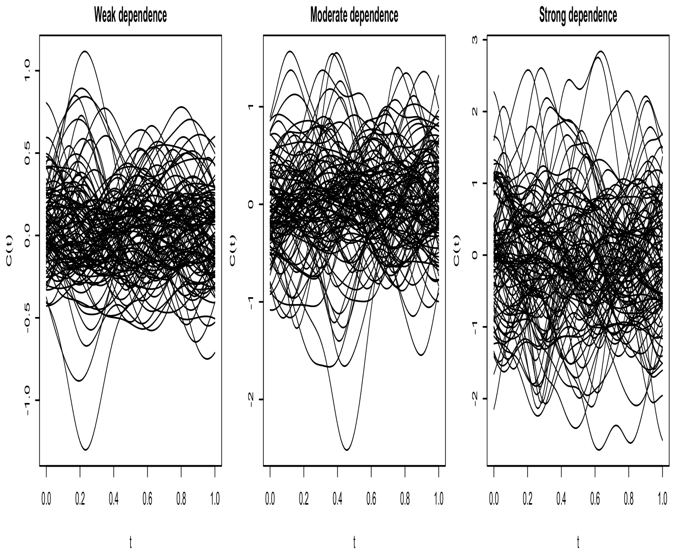
Three dependence scenarios were considered by varying the persistence parameters $(\alpha ,\beta )$, corresponding to weak $(0.10,0.60)$, moderate $(0.20,0.60)$, and strong $(0.25,0.70)$ temporal dependence. The simulated functional covariates under these three situations are presented in Figure 1.

The endogenous response variable D was generated according to the nonparametric regression model (3), where the regression operator is defined by

$$F_1\left(C\right)=4{\int }_0^{\pi }{\displaystyle \frac{C^2\left(t\right)}{1+C^2\left(t\right)}}dt.$$

To investigate the impact of the conditional variance on the performance of the proposed estimator, we considered three representative variance structures corresponding to increasing levels of heteroscedasticity:

$$F_2\left(C\right)=\left\{\begin{array}{cc}1,\hfill & (\mathrm{homoscedastic}\mathrm{model}),\hfill \\ {\displaystyle 1+0.5{\int }_0^{\pi }\left|C\left(t\right)\right|dt,}\hfill & (\mathrm{moderate}\mathrm{heteroscedasticity}),\hfill \\ {\displaystyle 1+{\int }_0^{\pi }{C}^2\left(t\right)dt,}\hfill & (\mathrm{strong}\mathrm{heteroscedasticity}).\hfill \end{array}\right.$$

The first specification corresponds to a constant conditional variance, whereas the second and third introduce progressively stronger heteroscedastic effects through functional characteristics of the covariate. This simulation design gives a comprehensive assessment of the robustness and stability of the proposed estimator.

For this empirical analysis, we compared two selectors for the smoothing parameter s that are

$$s_{Rule1}^{\mathrm{opt}}=arg\underset{s\in {\mathbf{H}}_n}{min}{\displaystyle \frac{1}{n}}{\displaystyle \sum _{i=1}^n}\left|{\displaystyle \frac{D_i-{\widehat{\theta }}^{-i}\left(C_i\right)}{D_i}}\right|,$$

(4)

and

$$s_{Rule2}^{\mathrm{opt}}=arg\underset{s\in {\mathbf{H}}_n}{min}{\displaystyle \frac{1}{n}}{\displaystyle \sum _{i=1}^n}\left|D_i-{\widehat{\theta }}^{-i}\left(C_i\right)\right|$$

(5)

where ${\widehat{\theta }}^{-i}$ denotes either the $\widehat{RAR}$ or the $\widetilde{RAR}$ estimator computed after removing the ith observation from the sample. To ensure a fair comparison, both bandwidth selection procedures were optimized over the same candidate set $H_n$.

For each selector, the optimal smoothing parameter s was chosen from $H_n$, which was constructed from the empirical quantiles of the pairwise distances between the Hilbert-valued covariates ${\left\{C_i\right\}}_{i=1}^n$. Specifically, the candidate values of s correspond to the empirical quantiles of orders

$$\left\{{\displaystyle \frac{1}{5}},{\displaystyle \frac{1}{10}},{\displaystyle \frac{1}{15}},{\displaystyle \frac{1}{2}}\right\}.$$

Finally, the estimator was implemented using a quadratic kernel with support on $(0,1)$. The similarity between functional covariates was measured through the PCA-based $L^2$ semi-metric, defined using the first three empirical eigenfunctions of the covariance operator associated with the three largest empirical eigenvalues (see Ferraty and Vieu [23]).

The predictive performance of the proposed estimation procedure was assessed by comparing the observed response values ${\left\{D_i\right\}}_{i=1}^n$ with their corresponding predictions ${\left\{\widehat{RAR}\left(C_i\right)\right\}}_{i=1}^n$ using the relative squared error (RSE), defined as

$$\mathrm{RSE}={\displaystyle \sum _{i=1}^n}{\displaystyle \frac{{\left(D_i-{\tilde{\theta }}^{-i}\left(C_i\right)\right)}^2}{D_i^2}},$$

where ${\tilde{\theta }}^{-i}\left(C_i\right)$ denotes the leave-one-out prediction of $D_i$.

The following algorithm summarizes the detailed procedure used in this part of the analysis:

Step 1.

Choose the level of dependence.

Step 2.

Choose the level of heteroscedasticity.

Step 3.

For the specified levels of dependence and heteroscedasticity and a given sample size n, generate a sequence of observations ${(D_i,C_i)}_{i=1,\dots ,150}$ according to model (3).

Step 4.

Split the sample in two parts: 80% of the observations were used as the training sample, while the remaining 20% were reserved for testing.

Step 5.

For each $s\in H_n$ and each observation i in the training sample we compute the estimators $\widehat{RAR}\left({\mathcal{C}}_i\right)$ and $\widetilde{RAR}\left({\mathcal{C}}_i\right)$ using the kernel and metric specified above.

Step 6.

For each observation i in the training sample we select the two optimal bandwidths according to the two bandwidth-selection rules defined in (4) and (5).

Step 7.

For each observation (j) in the testing sample, we compute the optimal estimators $\widehat{RAR}$ and $\widetilde{RAR}$ using the optimal bandwidths associated with its nearest observation in the training sample.

Step 8.

Compute the $\mathrm{RSE}$ of the optimal estimators $\widehat{RAR}$ and $\widetilde{RAR}$.

The algorithm was repeated over 150 independent Monte Carlo replications, and the average RSE was used to compare the competing estimation procedures. The corresponding prediction results are presented in

Table 1. The RSE for different scenarios.

Models	Dependency’s Level	Heteroscedasticity’s Level	Rules	RSE
$\widehat{RAR}$	Weak	Homoscedastic	rule 1	0.12
			rule 2	0.23
		Weak heteroscedasticity	rule 1	0.15
			rule 2	0.34
		Strong heteroscedasticity	rule 1	0.22
			rule 2	0.37
	Moderate	Homoscedastic	rule 1	0.31
			rule 2	0.43
		Weak heteroscedasticity	rule 1	0.37
			rule 2	0.46
		Strong heteroscedasticity	rule 1	0.39
			rule 2	0.53
	Strong	Homoscedastic	rule 1	0.41
			rule 2	0.57
		Weak heteroscedasticity	rule 1	0.52
			rule 2	0.61
		Strong heteroscedasticity	rule 1	0.58
			rule 2	0.66
$\widetilde{RAR}$	Weak	Homoscedastic	rule 1	0.41
			rule 2	0.73
		Weak heteroscedasticity	rule 1	0.67
			rule 2	0.85
		Strong heteroscedasticity	rule 1	0.92
			rule 2	1.08
	Moderate	homoscedastic	rule 1	1.13
			rule 2	1.23
		Weak heteroscedasticity	rule 1	1.17
			rule 2	1.34
		Strong heteroscedasticity	rule 1	1.24
			rule 2	1.46
	Strong	Homoscedastic	rule 1	1.44
			rule 2	1.56
		Weak heteroscedasticity	rule 1	1.72
			rule 2	1.81
		Strong heteroscedasticity	rule 1	1.78
			rule 2	1.96

.

The results presented in Table 1 indicate that the proposed estimator, $\widehat{RAR}$ outperforms its competitor, $\widetilde{RAR}$ in terms of estimation accuracy. More importantly, $\widehat{RAR}$ exhibits remarkably low error variability across the various simulated scenarios, whereas the performance of $\widetilde{RAR}$ has more fluctuation. This stable behavior is especially observed under heteroscedastic conditions, which pose a more complex modeling challenge. Given that the robustness of a regression estimator is evaluated by its capacity to deliver stable predictions despite changing data structures, the minimal variance in the error of $\widehat{RAR}$ offers a good evidence of its superior robustness and practical utility in heterogeneous environments.

Now, in order to assess the consistency and the stability of the proposed estimator, we compare its performance with two standard benchmark approaches: the mean regression and the median regression. Such models are, respectively, estimated by

$$\widehat{MEA}\left(\mathcal{C}\right)={\displaystyle \frac{{\displaystyle {\displaystyle \sum _{i=1}^n}\mathcal{N}\left(s^{-1}\mathcal{S}(\mathcal{C},C_i)\right)D_i}}{{\displaystyle {\displaystyle \sum _{i=1}^n}\mathcal{N}\left(s^{-1}\mathcal{S}(\mathcal{C},C_i)\right)}}}.$$

and

$$\widehat{MED}\left(\mathcal{C}\right)=arg\underset{d}{min}{\displaystyle \frac{{\displaystyle {\displaystyle \sum _{i=1}^n}\mathcal{N}\left(s^{-1}\mathcal{S}(\mathcal{C},C_i)\right)\left|D_i-d\right|}}{{\displaystyle {\displaystyle \sum _{i=1}^n}\mathcal{N}\left(s^{-1}\mathcal{S}(\mathcal{C},C_i)\right)}}}.$$

For the sake of brevity, we focus on the most challenging simulation scenario, characterized by strong dependence and strong heteroscedasticity. This choice is motivated by the fact that, if an estimator maintains reliable performance under strong dependence and substantial heteroscedasticity, this provides stronger evidence of its robustness. Under this challenging setting, we compare the three regression approaches across a different of sample sizes $n=50,100,250,300$. The conditional mean and median regressions are computed using the corresponding routines fregre.np.cv and cond.quantile, available in the R package fda.usc. This comparison therefore provides a complementary assessment of the finite-sample behavior and practical reliability of the proposed estimator relative to standard regression methods. We follow the same algorithm described above under the rule 1 to compute $\widehat{RAR}$. We report the resulting $\mathrm{RSE}$ values in the following

Table 2. The RSE for different models.

n	$\mathit{RSE}\left(\widehat{\mathit{RAR}}\right)$	$\mathit{RSE}\left(\widehat{\mathit{MED}}\right)$	$\mathit{RSE}\left(\widehat{\mathit{MEA}}\right)$
50	0.71	0.98	1.56
100	0.63	0.82	1.41
250	0.54	0.78	1.37
300	0.52	0.73	1.32
400	0.51	0.67	1.25

.

The results in Table 2 show that $\widehat{RAR}$ achieves the lowest $\mathrm{RSE}$ for all sample sizes, indicating better estimation accuracy than mean regression and median regression. Its $\mathrm{RSE}$ decreases from $0.71$ to $0.51$ as n increases. However, the performance remains stable for n large. The conditional median estimator $\widehat{MED}$ also benefits from larger sample sizes, but its error remains systematically higher than that of $\widehat{RAR}$. Overall, these results highlight the good accuracy and stable performance of $\widehat{RAR}$, namely under the challenging combination of strong dependence and strong heteroscedasticity.

6. A Real Data Application

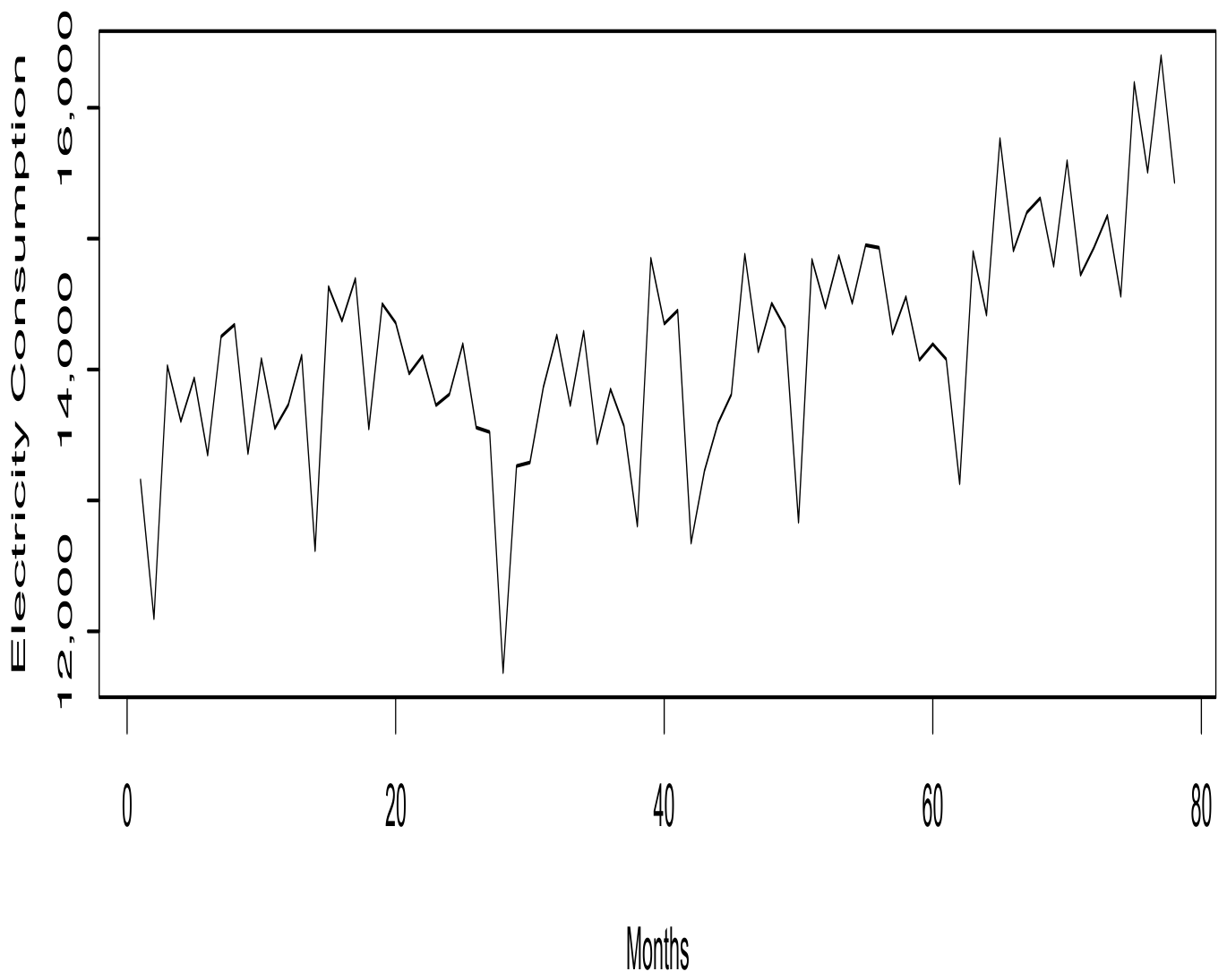
In this section, we illustrate the practical applicability of the proposed methodology through the analysis of a real world dataset. Specifically, we consider the monthly electricity consumption data for Malaysia, which are publicly available at https://storage.data.gov.my/energy/electricity_consumption.csv (accessed on 18 July 2026). The use of this type of data is motivated by its naturally heterogeneous structure, which is often associated with substantial seasonal variation and possible structural changes in electricity demand. In particular, electricity consumption may vary considerably across months and seasons due to changes in weather conditions, economic activity, and consumer behavior. Such variations can lead to high variability over time, making electricity demand a relevant and realistic setting for assessing the performance and robustness of regression methods under heteroscedasticity. Furthermore, the considered dataset consists of 80 monthly observations during the period from January 2018 to December 2024. The corresponding electricity consumption curve is presented in Figure 2.

Our objective is to predict the monthly electricity consumption one month ahead using the observations from the preceding 12 months. A similar analysis of this dataset was conducted by Ferraty and Vieu [23] in the framework of functional data analysis using the classical nonparametric regression mode after transforming the original time series by applying a logarithmic difference. This transformation is important for ensuring the stationarity of the data.

Although conventional regression methods perform well under standard Gaussian assumptions, electricity consumption data often exhibit complex dynamics driven by structural changes, extreme weather conditions, and unexpected economic events. Such factors typically induce heavy-tailed distributions and produce atypical observations that can substantially affect the predictive performance of least-squares-based methods. So, to overcome these limitations, we propose a functional regression approach based on the Least Absolute Relative Error (LARE) criterion. The LARE model is particularly attractive because of its scale invariance and its robustness to outliers. Indeed, the $L_1$-type relative loss penalizes large deviations linearly rather than quadratically, reducing the influence of extreme observations on the fitted model.

To demonstrate the advantages of the proposed approach, we compare the LARE estimator with both the Least Squares Relative Error (LSRE) model and the standard Nadaraya–Watson Conditional Expectation (NWCE) estimator, $m\left(\mathcal{C}\right)=\mathrm{I}\mathrm{E}[D\mid C=\mathcal{C}].$ Specifically, the kernel estimator associated with the traditional LSRE model, denoted by $\widehat{{\mathcal{N}}_1}\left(\mathcal{C}\right)$, is defined as follows:

$${\displaystyle \widehat{{\mathcal{N}}_1}\left(\mathcal{C}\right)=\frac{{\sum }_{i=1}^n\mathcal{N}\left(h_n^{-1}d(\mathcal{C},C_i)\right)D_i^{-1}}{{\sum }_{i=1}^n{D}_i^{-2}\mathcal{N}\left(h_n^{-1}d(\mathcal{C},C_i)\right)},}$$

(6)

whereas the classic kernel or Nadraya-Watson-Conditional-Expectation (NWCE) $\widehat{m_2}\left(\mathcal{C}\right)$ is defined as:

$${\displaystyle \widehat{{\mathcal{N}}_2}\left(\mathcal{C}\right)=\frac{{\sum }_{i=1}^n\mathcal{N}\left(h_n^{-1}d(\mathcal{C},C_i)\right)D_i}{{\sum }_{i=1}^n\mathcal{N}\left(h_n^{-1}d(\mathcal{C},C_i)\right)}.}$$

(7)

Now, for this experiment, we keep the notations of the preceding sections we denote by $Q_t$ the monthly electricity consumption time series observed over a horizon of 80 months.

The monthly electricity consumption data are organized into functional units by using each consecutive block of 12 monthly observations to construct a functional curve. This segmentation provides a natural functional representation of the annual consumption, with each curve describing the evolution of electricity demand over a one year period. Using this representation, we aim to predict the consumption during the last 12 months, corresponding to the 68th functional segment, based on the preceding 67 segments used as the training sample. More specifically, for each fixed target month j in the last year, we construct the functional regression sample from the pairs ${(D_i^j,C_i^j)}_{(i=1)}^{67}$, where $C_i^j$ is the functional predictor obtained from the 12 monthly electricity consumption observations preceding month j, and $D_i^j$ is the scalar electricity consumption observed in month. This formulation allows the same functional covariate $C_i$ to be used to predict each of the 12 monthly consumption values separately, while preserving the dependence structure within the annual consumption profiles. Furthermore, to investigate the robustness of the estimators, we perform a comparative study across two distinct data regimes:

1.

Contamination-Free Regime (Absence of Outliers): The models are trained on the stationary, log-differenced transformation introduced by Ferraty and Vieu [23]. This baseline scenario evaluates performance under standard, well-behaved structural conditions.

2.

Contaminated Regime (Presence of Outliers): Artificial anomalies are introduced into the dataset by arbitrarily scaling some percentage p of the response variables ($D_i^j$) by a factor of M. This heavy-tailed contamination explicitly challenges the model sensitivities to extreme leverage points.

In both experimental settings, the functional predictor is endowed with the semi-metric induced by the principal component representation of the functional data. Specifically, the semi-metric is constructed by projecting the curves onto the m first principal components associated with the largest eigenvalues of the empirical covariance operator. Nonparametric smoothing is performed using the quadratic (Epanechnikov) kernel,

$$\mathcal{N}\left(x\right)={\displaystyle \frac{3}{2}}(1-x^2){\mathbf{1}}_{[0,1]}\left(x\right).$$

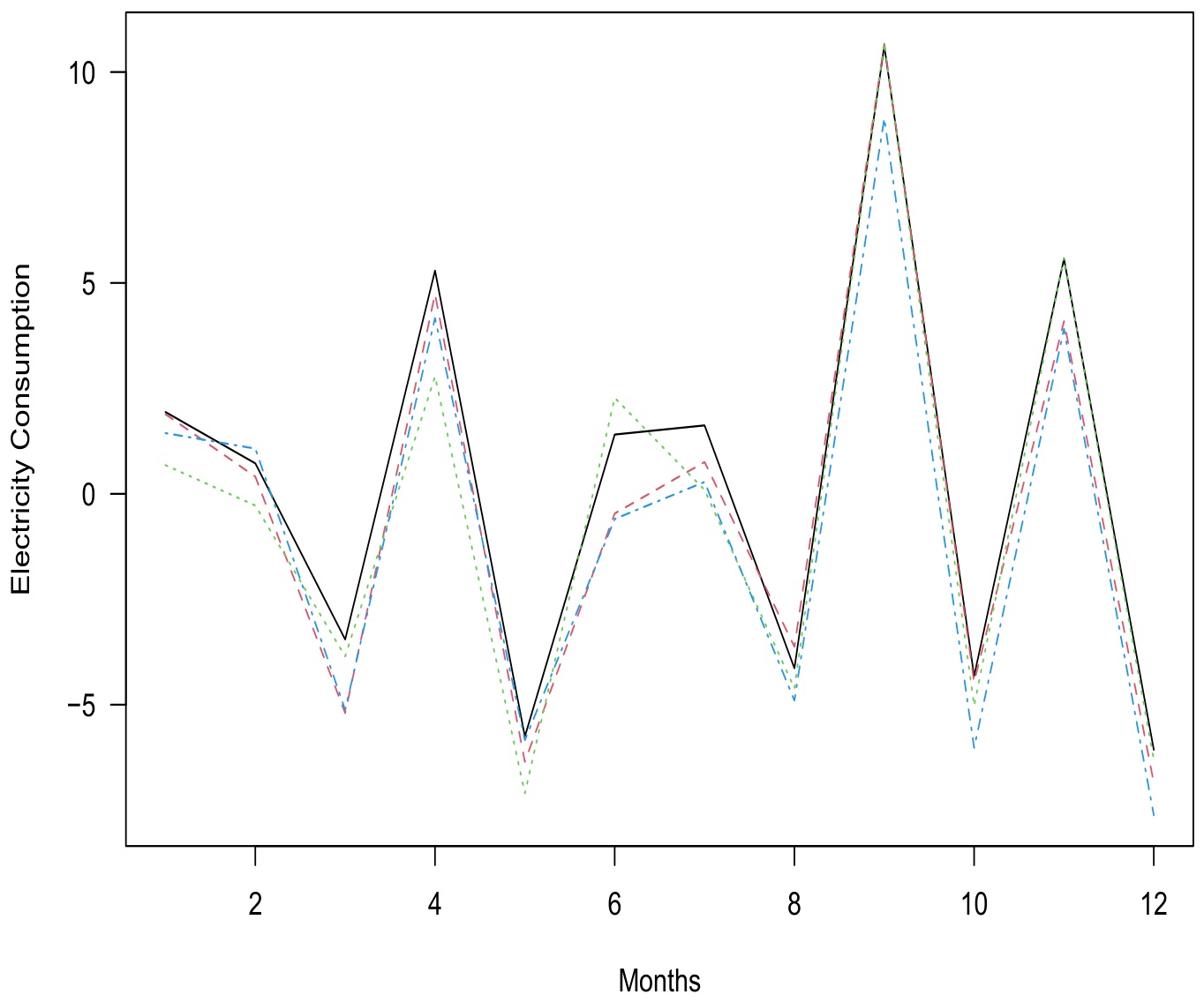
The structural tuning parameters, namely the number of principal components m defining the semi-metric and the local smoothing bandwidth s, are selected automatically through a data-driven cross-validation procedure based on the criterion given in (4). The resulting prediction curves are displayed in Figure 3 where the observed electricity consumption series is represented by a solid line, while the corresponding predictions obtained from the competing models are shown by dashed lines.

An examination of the forecasting results presented in Figure 3 confirms the effectiveness of the proposed functional prediction framework. In the absence of anomalous observations, both the classical least-squares relative error (LSRE) regression and the proposed Least Absolute Relative Error (LARE) regression provide highly accurate forecasts. To assess predictive performance, we compute the mean absolute error (MAE), defined by

$$\mathrm{MAE}={\displaystyle \frac{1}{12}}{\displaystyle \sum _{j=1}^{12}}\left|D_i\left(j\right)-\mathrm{Pred}\left(C_i\right)\left(j\right)\right|,$$

where $\mathrm{Pred}$ denotes the prediction obtained from the LARE, LSRE, or Nadaraya–Watson conditional expectation (NWCE) model.

The obtained MAE values are $0.59$ for the proposed LARE estimator, compared with $0.87$ for the LSRE estimator and $0.95$ for the NWCE estimator. These results indicate that the proposed LARE approach achieves the highest predictive accuracy, even under regular operating conditions where no prominent outliers are present. This demonstrates that the scale-invariant relative loss underlying the LARE criterion preserves predictive efficiency while avoiding the sensitivity to large deviations that characterizes conventional least-squares-based methods.

In contrast, the superiority of the proposed LARE framework becomes particularly evident under the contaminated data setting. See the MAE reported in

Table 3. The $\mathrm{MAE}$ for different models under different contamination level.

M	p	$\mathit{MAE}(\widehat{\mathit{RAR}})$	$\mathit{MAE}(\widehat{{\mathcal{N}}_1})$	$\mathit{MAE}(\widehat{{\mathcal{N}}_2})$
5	10%	0.60	1.08	1.26
5	20%	0.60	1.14	1.67
5	30%	0.61	1.25	1.74
10	10%	0.61	1.29	2.12
10	20%	0.63	1.37	2.25
10	30%	0.64	1.52	2.41
100	10%	0.62	1.79	2.58
100	20%	0.65	1.83	2.62
100	30%	0.65	1.98	2.67

.

The robustness and stability of the proposed LARE regression are particularly evident under the contaminated data case, as shown in Table 3 and Figure 4. Unlike the competing methods, whose prediction errors increase with the the contamination level, the LARE estimator maintains a stable performance. For instance, when $M=100$, its MAE changes only slightly, from $0.62$ at a contamination level of $10\%$ to $0.65$ at $30\%$. The same stability is observed for $M=5$ and $M=10$, where the MAE varies only within the narrow ranges $[0.60,0.61]$ and $[0.61,0.64]$, respectively. In contrast, the MAE of ${\mathcal{N}}_1$ and ${\mathcal{N}}_2$ increases substantially with the contamination level, particularly when $M=100$. Thus, the small variation in the LARE error across different contamination levels provides clear evidence of its robustness to anomalous observations. This stability confirms that the relative absolute error successfully limits the influence of extreme observations, allowing the proposed regression to preserve its predictive accuracy even when the data are increasingly contaminated.

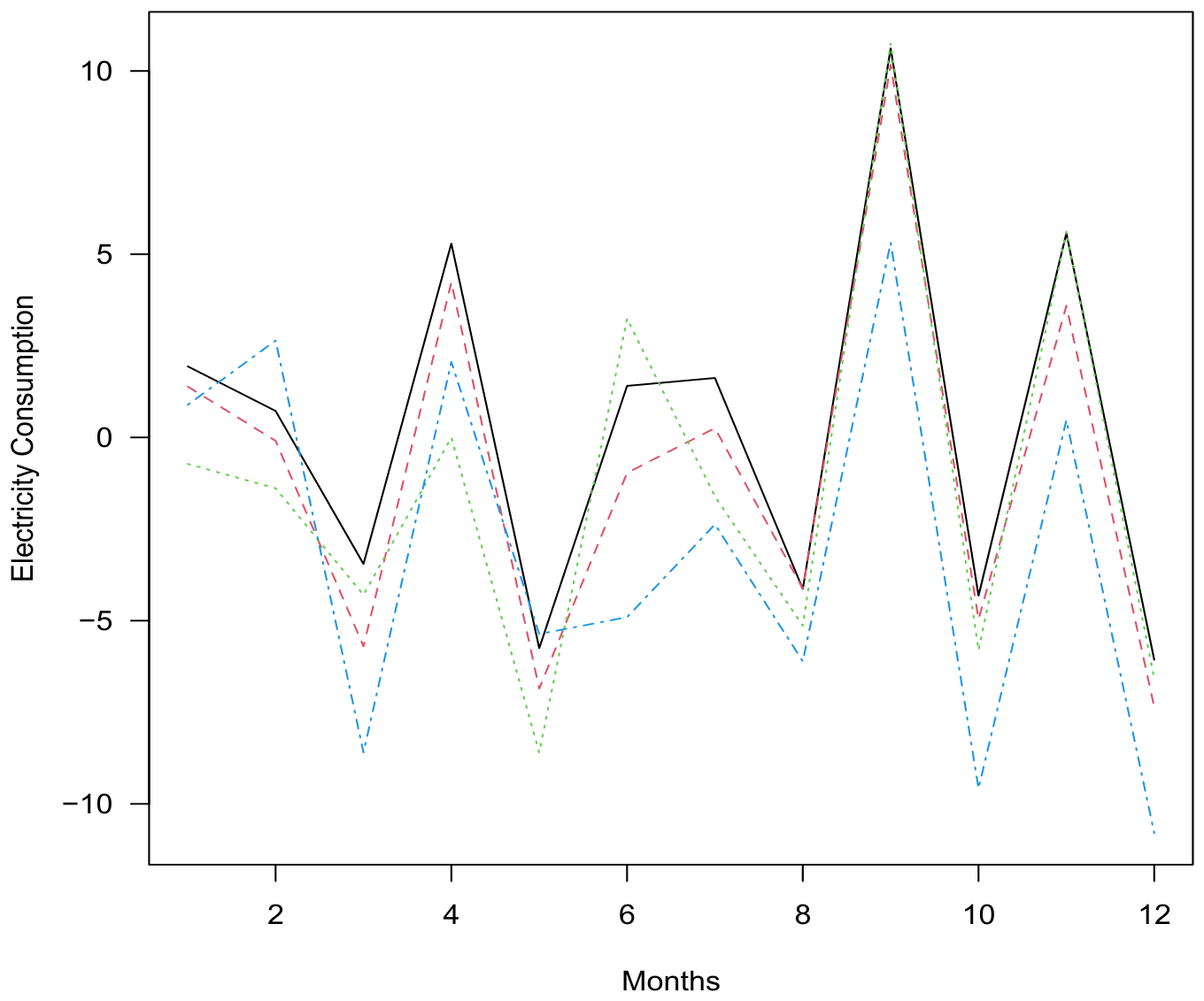
To visualize the advantage of the proposed LARE regression over its main competitors, the LSRE and Nadaraya–Watson conditional expectation (NWCE) estimators, Figure 4 presents their prediction results under the most challenging contamination scenario considered in Table 3. Specifically, the figure corresponds to the last row of the table, where $M=100$ and $30\%$ of the observations are contaminated.

Once again the graphical results provide a clear illustration of the robustness and stability of the LARE estimator. Despite the severe contamination, the LARE predictions remain close to the observed curve and preserve its main features, with only minor deviations. In contrast, the predictions produced by the LSRE and NWCE estimators are visibly more affected by the contaminated observations. This difference is consistent with the numerical results reported in Table 3, where the MAE of LARE remains stable, while the errors of the competing methods increase substantially. Overall, the figure provides complementary visual evidence that the proposed LARE regression is less sensitive to extreme observations and maintains reliable predictive performance even in the presence of a high level of contamination. Finally, let us point out that the stationarity is a fundamental condition for establishing our theoretical results. In this real data application, stationarity is ensured by considering the differences of the logarithmic series. This transformation is commonly used in financial time-series analysis to remove stochastic trends and stabilize the mean and variance of the series. Moreover, we have confirmed this aspect by the Dickey–Fuller (ADF) test, through the adf.test routine in R. Since our observations are functional, the test was applied to the leading principal component scores obtained from the functional observations. The results provide empirical evidence supporting the stationarity of the transformed functional time series. However, to assess the impact of this aspect on forecasting performance, we compare the three models using the original data without applying the stationarity transformation. The results show a substantial difference in predictive performance between the transformed and untransformed cases. In particular, the obtained MAE values are 1087 for the proposed LARE estimator, compared with 2695 for the LSRE estimator and 3957 for the NWCE estimator. These considerably larger prediction errors highlight the practical importance of the stationarity assumption for achieving accurate and reliable forecasts and provide empirical support for the use of the proposed methodology under stationary data.

7. Conclusions and Prospects

This paper extends the functional Least Absolute Relative Error (LARE) regression framework to the more challenging setting of dependent functional observations, where the explanatory variables form a functional time series. This extension represents a significant generalization of the existing theory, since temporal dependence introduces additional technical difficulties in both the estimation procedure and the asymptotic analysis. To address these challenges, we develop a new kernel-based LARE estimator for functional time series and establish its main asymptotic properties, including asymptotic normality under suitable weak dependence conditions. As in the independent setting, the functional structure is characterized through the small-ball probability function, which explores the local concentration of the probability measure in infinite-dimensional spaces. The use of the LARE loss further provides a robust estimation framework that is considerably less sensitive to atypical observations and heavy-tailed distributions than classical least-squares approaches.

The theoretical results are established under mild and flexible assumptions allowing to include a large class of stationary functional time series. In particular, the mixing condition provides a general framework for controlling the temporal dependence between functional observations that are sufficiently separated in time, while still allowing for substantial dependence at shorter lags. Consequently, the proposed methodology applies to a wide range of dependent functional data arising in economics, finance, environmental sciences, energy systems, and other applications where serial dependence is an intrinsic feature of the observed curves. From a practical point of view, the assumed dependence structure in finite-dimensional case can be assessed empirically using diagnostic tools available in standard statistical software such as Autocorrelation Function ACF in R-package stats. For functional observations, this problem can be done by applying autocorrelation-type measures to suitable scalar summaries by principal component scores obtained from the curves. However, constructing a practical tool to verify the strong mixing condition remains an open question for future research. Of course the construction of this partiocal tool enhances the feasibility of our model. Overall, the practical value of the proposed methodology is illustrated through the analysis of a real monthly electricity consumption dataset. The empirical study compares the proposed functional LARE predictor with the functional Least Squares Relative Error (LSRE) estimator and the classical functional Nadaraya–Watson conditional expectation predictor. When the data are free from anomalous observations, all competing methods provide satisfactory forecasts, with the proposed LARE estimator achieving the smallest prediction error. Its advantage becomes substantially more pronounced in the presence of contaminated observations, where the predictive performance of the least-squares-based methods deteriorates markedly, whereas the LARE estimator remains stable and accurate. These results clearly demonstrate that the proposed approach successfully combines predictive efficiency with robustness, making it particularly suitable for forecasting functional time series exhibiting outliers or heavy-tailed behaviour.

Several directions deserve further investigation. An important extension is the development of robust functional LARE estimators based on local k-nearest-neighbour smoothing or semiparametric regression models for dependent functional data. Another promising research direction concerns the analysis of partially observed or incomplete functional time series. Extending the proposed methodology to accommodate missing or censored trajectories would further enhance its practical applicability and could be developed by combining the LARE framework with modern techniques for incomplete functional data, including likelihood-based approaches, inverse-probability weighting, and semiparametric estimation methods.