Motion in the ER3BP Under a Heterogeneous Triaxial Primary and a Modified Newtonian Force of the Secondary

Abstract

This paper investigates the dynamical behaviour of an infinitesimal mass body moving under the gravitational influence of a heterogeneous triaxial primary body and a secondary body that produces a modified Newtonian gravitational force in the elliptic restricted three-body problem. In this model, the two primary bodies move around their common center of mass in elliptical orbits, while the mass of the third body is assumed to be sufficiently small so that its effect on the motion of the primary bodies can be neglected. The equations of motion of the infinitesimal body are formulated, and the corresponding mean motion of the system is determined by taking into account the triaxial structure and mass heterogeneity of the primary body as well as the modified gravitational field of the secondary. The equilibrium points of the system are then investigated. Both collinear equilibrium points, which lie along the line joining the two primary bodies, and non-collinear equilibrium points, which are located away from this line, are determined analytically. Their linear stability is examined by studying the characteristic equations associated with small perturbations around these points. In addition, the dynamical characteristics of the system are illustrated numerically through potential surfaces, the locations of equilibrium points, permissible regions of motion, periodic orbits, and basins of attraction. These numerical results provide a clear understanding of how the eccentricity of the motion, triaxiality of the primary body, and the modified gravitational force of the secondary influence the motion of the infinitesimal body. The results may be useful in understanding the dynamics of celestial bodies.

1. Introduction

Celestial mechanics and dynamical astronomy is a branch of applied mathematics and applied physics. Firstly, Newton solved the two-body problem, the problem of calculating the motion of the Earth around the Sun by giving the inverse-square law of gravitational attraction between them. After this, many mathematicians and physicists tried to extend Newton’s methods to the three-body problem, but after decades, it was realized that solving the three-body problem was impossible. Thereafter, the restricted three-body problem took its place, where out of three bodies, two bigger bodies are placed at the same line and moving in the either circular or elliptic orbits in the same plane around their center of mass while the third smallest (infinitesimal mass) body is moving under the gravitational effects of the two bigger bodies without affecting their motion. In this way, many researchers have investigated the circular restricted three-body problem (CR3BP) and elliptical restricted three-body problem (ER3BP).

The authors of [1] explored the idea of the two-body motions, the restricted three-body problem in two and three dimensions, and many more. Ref. [2] numerically explored the simple periodic symmetrical orbits in Hill’s limiting case and the stability of the Lagrange points. The author found that these points are unstable. Ref. [3] investigated numerically the locations of the five equilibrium points by assuming the effect of oblateness of the more massive primary for some systems. They also investigated the characteristic exponents in two-dimensional and three-dimensional restricted three-body problems. Ref. [4] studied numerically the non-linear stability of motions around non-collinear equilibrium points in the ER3BP under the effect of orbital eccentricity. The authors observed that on an increase in eccentricity, the width of stability regions decreases.

Ref. [5] gave the stability regions for the out-of-plane equilibrium points in the circular restricted three-body problem. The authors also computed the second-order expansions of periodic solutions and observed that out of two families, one starts and ends at the same points, while the other ends on the orbital plane. Ref. [6] investigated the linear stability and the resonance cases for the non-collinear equilibrium points in the photo-gravitational elliptic R3BP. The authors observed that third- and fourth-order resonances exist. Ref. [7] examined the effect of solar radiation pressure on the motion of a test particle around the non-collinear equilibrium points in the circular R3BP. The authors also constructed the second-order parametric expansions by which the family of periodic orbits are illustrated numerically in two cases: resonant and non-resonant. Ref. [8] investigated the resonant case with new results in the elliptic R3BP.

Ref. [9] illustrated four resonant families of periodic orbits in the planar elliptic restricted three-body problem. The authors also compared CR3BP with ER3BP in the resonant cases. Ref. [10] explained many aspects of the restricted problems. Ref. [11] investigated the existence and stability of equilibrium points in the circular restricted three-body problem by assuming primaries as triaxial rigid bodies. The authors also considered that the equatorial plane coincides with the plane of motion. They revealed that the triangular points have long or short periodic elliptical orbits for some value of the mass parameter. Ref. [12] obtained the solutions for the angular velocities and pressures of a heterogeneous oblate spheroid by solving the Euler hydrodynamical equations. Ref. [13] examined the stability of libration points in the elliptic restricted three-body problem for different values of eccentricity by assuming that the primary bodies having source of radiation pressure. Ref. [14] illustrated the periodic motion and stability around the collinear equilibrium points in the CR3BP by assuming the primary as a source of radiation pressure and secondary as an oblate body.

Ref. [15] investigated the effect of oblateness on the motion of a test particle in the three-dimensional photo-gravitational restricted three-body problem. Ref. [16] illustrated the periodic orbits around the non-collinear equilibrium points under the influence of various perturbations such as the effects of oblateness, radiation pressure, and Coriolis and centrifugal forces. The authors also showed the effects of perturbations on the long and short periodic orbits. Refs. [17,18] investigated the circular restricted three-body problem with various perturbations, like Yarkovsky effects, photo-gravitational effects, etc. Ref. [19] studied the effect of oblateness of Saturn on the motion of the infinitesimal body in the circular R3BP where the primary is taken as Saturn and secondary is considered as Titan. The authors made numerical investigations of periodic orbits by utilizing the numerical technique of Poincaré surfaces of sections. They observed that periodic orbits converted to quasi-periodic orbits due to the effects of oblateness.

Other researchers have also investigated the restricted problem by considering either circular or elliptic orbits of the primaries, for example, Refs. [20,21,22,23,24,25,26,27,28].

In view of the above literature, we have been motivated to investigate the elliptic restricted three-body problem with heterogeneous primary and modified Newtonian secondary.

The rest of the paper is organized as follows: The model of the problem and equations of motion are presented in Section 2 while Section 3 presents the mean motion of the system. The analytical investigations are made in Section 4, while the numerical explorations are presented in Section 5.1, Section 5.2, Section 5.3, Section 5.4, Section 5.5 and Section 5.6. The paper concludes in Section 6.

2. Equations of Motion

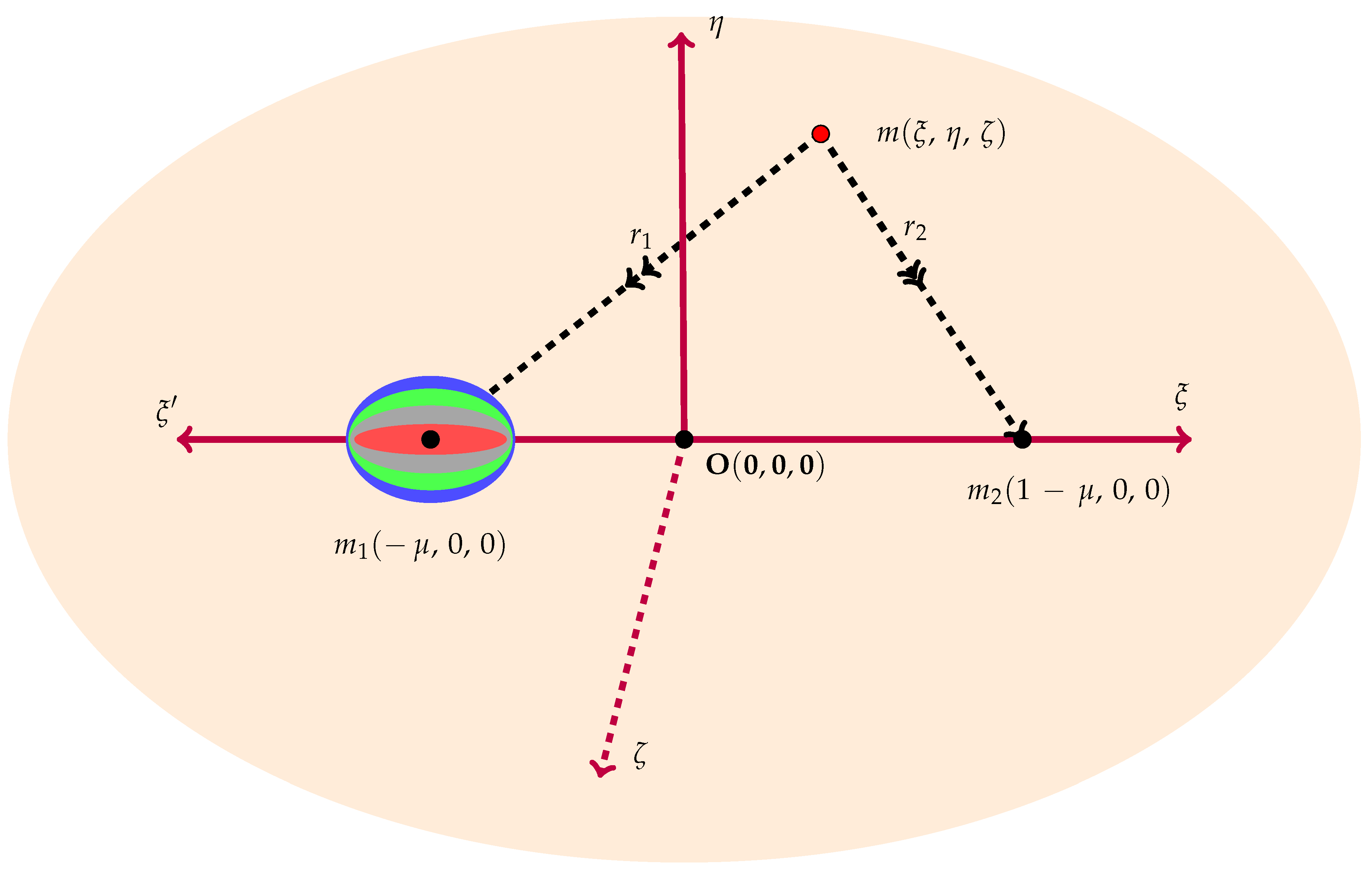
On assumption of the elliptic restricted three-body problem where two primary bodies are placed on the ${\displaystyle \xi }$-axis (where ${\displaystyle \xi \eta \zeta }$-axes follow the right hand rule). Out of these two bodies, one is of a heterogeneous triaxial shape with N-layers of different densities and the other is of a spherical shape having a modified Newtonian potential. In addition, both bodies are moving in elliptic orbits about their common center of mass, which is taken as the origin of the reference frame as well. The third infinitesimal mass body is moving in the space under the gravitational forces of the primary bodies. The complete configuration of the problem can be seen in Figure 1. The equations of motion of an infinitesimal mass (third body) in a normalized system of units and a rotating-pulsating reference frame, can be presented by following [29,30,31] as:

$$\begin{array}{ccc}{\xi }^{″}-2{\eta }^{\prime }\hfill & =& {\mathsf{\Omega }}_{\xi },\hfill \\ {\eta }^{″}+2{\xi }^{\prime }\hfill & =& {\mathsf{\Omega }}_{\eta },\hfill \\ {\zeta }^{″}\hfill & =& {\mathsf{\Omega }}_{\zeta },\hfill \end{array}$$

(1)

with

$$\begin{array}{ccc}\mathsf{\Omega }\hfill & =& {(1-e^2)}^{-{\displaystyle \frac{1}{2}}}\left[{\displaystyle \frac{1}{2}}({\xi }^2+{\eta }^2)+{\displaystyle \frac{1}{n^2}}\left({\displaystyle \frac{1-\mu }{r_1}}+{\displaystyle \frac{k_1}{2r_1^3}}-{\displaystyle \frac{3k_2{\eta }^2}{2r_1^5}}+{\displaystyle \frac{\mu r_2}{r_2^2+\delta }}\right)\right],\hfill \\ r_1^2\hfill & =& {(\xi +\mu )}^2+{\eta }^2+{\zeta }^2,r_2^2={(\xi +\mu -1)}^2+{\eta }^2+{\zeta }^2,\hfill \\ k_1\hfill & =& {\displaystyle \frac{4\pi }{3}}{\displaystyle \sum _{i=1}^N}\left[({\delta }_i-{\delta }_{i+1})A_i{B}_i{C}_i{\sigma }_{i,1}\right],k_2={\displaystyle \frac{4\pi }{3}}{\displaystyle \sum _{i=1}^N}\left[({\delta }_i-{\delta }_{i+1})A_i{B}_i{C}_i{\sigma }_{i,2}\right],\hfill \\ {\sigma }_{i,1}\hfill & =& {\displaystyle \frac{2A_i^2-B_i^2-C_i^2}{5}},{\sigma }_{i,2}={\displaystyle \frac{A_i^2-B_i^2}{5}},\hfill \end{array}$$

(2)

${\displaystyle \delta =G{m}_1{m}_2{\pi }_1}$, ${\displaystyle |{\pi }_1|<<1}$ is a parameter representing the perturbed force of the continued fractional potential by which the Newtonian potential force is modified.

${\displaystyle k_3={\displaystyle \frac{{\sum }_{i=1}^N\left\{({\delta }_i-{\delta }_{i+1})A_i{B}_i{C}_i{\sigma }_{i1}\right\}}{{\sum }_{i=1}^N\left\{({\delta }_i-{\delta }_{i+1})A_i{B}_i{C}_i\right\}}},k_{1,2}<<1,A_i=\frac{a_i}{R},B_i=\frac{b_i}{R},C_i=\frac{c_i}{R}}$, ${\displaystyle {\delta }_{N+1}=0}$, ${\displaystyle {\delta }_i=\frac{{\rho }_i}{M}, M=m_1+m_2,}$ ${\displaystyle m_1}$ is the mass of the heterogeneous triaxial primary with N layers of densities ${\displaystyle {\rho }_i}$ and semi-axes ${\displaystyle (a_i,b_i,c_i),}$ ${\displaystyle i=1,2,3,4,\dots \dots ,N,}$ ${\displaystyle {\rho }_i<{\rho }_{i+1},}$ ${\displaystyle a_i<a_{i+1},}$ ${\displaystyle b_i<b_{i+1},}$ ${\displaystyle c_i<c_{i+1}.}$ ${\displaystyle m_2}$ is the mass of the secondary influenced by modified Newtonian potential. ${\displaystyle r_1}$ and ${\displaystyle r_2}$ are distances of the infinitesimal mass from the primary and secondary, respectively, while a and e are, respectively, the semi-major axis and eccentricity of the orbits. ${\displaystyle \mu =\frac{m_2}{m_1+m_2}\le \frac{1}{2},}$ ${\displaystyle m_1\ge m_2,}$ ${\displaystyle m_1=1-\mu ,m_2=\mu .}$ ${\displaystyle ({\xi }_1=-\mu ,0,0),}$ ${\displaystyle ({\xi }_2=1-\mu ,0,0)}$ and ${\displaystyle (\xi ,\eta ,\zeta )}$ are the coordinates of the primary and secondary and the third infinitesimal body, respectively. R is the dimensional distance between the primary and the secondary. n is the mean motion of the primary bodies, which is determined in the next section.

3. Mean Motion

The potential between a heterogeneous triaxial primary of mass ${\displaystyle m_1}$ with N layers of different densities ${\displaystyle {\rho }_i}$ and a secondary of mass ${\displaystyle m_2}$ with a modified Newtonian potential can be expressed as [32]

$$V=-{\displaystyle \frac{G{m}_1{m}_{2}R}{R^2+\delta }}-{\displaystyle \frac{G{m}_2{k}_1^{\ast }}{2R^3}},$$

where R is the distance between the primaries on the ${\displaystyle \xi }$-axis, G is the universal gravitational constant, ${\displaystyle m_1=\frac{4\pi }{3}{\displaystyle \sum _{i=1}^N}({\rho }_i-{\rho }_{i+1})a_i{b}_i{c}_i,}$ ${\displaystyle k_1^{\ast }=\frac{4\pi }{3}{\displaystyle \sum _{i=1}^N}({\rho }_i-{\rho }_{i+1})a_i{b}_i{c}_i{\sigma }_{i1}^{\ast },}$ ${\displaystyle {\sigma }_{i1}^{\ast }={\displaystyle \frac{2a_i^2-b_i^2-c_i^2}{5}},}$ and other symbols have their usual meanings.

Therefore, the force between ${\displaystyle m_1}$ and ${\displaystyle m_2}$ is

$$F={\displaystyle \frac{\partial V}{\partial R}}={\displaystyle \frac{G{m}_1{m}_2(R^2-\delta )}{{(R^2+\delta )}^2}}+{\displaystyle \frac{3G{m}_2{k}_1^{\ast }}{2R^4}}.$$

In the elliptic two-body problem, the variable distance between ${\displaystyle m_1}$ and ${\displaystyle m_2}$ is

$$r={\displaystyle \frac{a(1-e^2)}{(1+eCos\nu )}},$$

where ${\displaystyle \nu }$ is the true anomaly and the mean distance between them [29]

$$R={\displaystyle \frac{1}{2\pi }}{\int }_0^{2\pi }rd\nu ={\displaystyle \frac{a(1-e^2)}{{(1+e^2)}^{1/2}}}.$$

Furthermore, with respect to the center of mass, the orbits of ${\displaystyle m_1}$ and ${\displaystyle m_2}$ with semi-major axes ${\displaystyle a_1=a\mu }$ and ${\displaystyle a_2=a(1-\mu )}$, respectively, have same eccentricity ${\displaystyle e}$ [1].

Therefore, by using

$$\ddot{R}-R{\dot{\theta }}^2=-f\left(R\right),$$

the equations of motion of ${\displaystyle m_1}$ and ${\displaystyle m_2}$ can be written as

$$\begin{array}{ccc}a\mu n^2{\displaystyle \frac{(1-e^2)}{{(1+e^2)}^{1/2}}}\hfill & =& {\displaystyle \frac{G{m}_2(R^2-\delta )}{{(R^2+\delta )}^2}}+{\displaystyle \frac{3G{m}_2{k}_1^{\ast }}{2R^4{m}_1}},\hfill \end{array}$$

(3)

and

$$\begin{array}{ccc}a(1-\mu )n^2{\displaystyle \frac{(1-e^2)}{{(1+e^2)}^{1/2}}}\hfill & =& {\displaystyle \frac{G{m}_1(R^2-\delta )}{{(R^2+\delta )}^2}}+{\displaystyle \frac{3G{k}_1^{\ast }}{2R^4}}.\hfill \end{array}$$

(4)

Adding Equations (3) and (4), and then using ${\displaystyle m_1+m_2=1,R=1=a,}$ ${\displaystyle \frac{k_1^{\ast }}{m_1}=k_3<<1,}$ we have

$$\begin{array}{ccc}{n}^2\hfill & =& {\displaystyle \frac{{(1+e^2)}^{1/2}}{a(1-e^2)}}\left\{{\displaystyle \frac{3k_3}{2}}+{\displaystyle \frac{1-\delta }{{(1+\delta )}^2}}\right\},\hfill \end{array}$$

(5)

after neglecting second and higher powers of ${\displaystyle e^2}$, ${\displaystyle \delta }$, ${\displaystyle k_3}$ and their products, we obtain

$$\begin{array}{ccc}{n}^2\hfill & =& {\displaystyle \frac{1}{a}}\left(1+{\displaystyle \frac{3}{2}}{e}^2+{\displaystyle \frac{3}{2}}{k}_3-3\delta \right).\hfill \end{array}$$

(6)

This is the required mean motion of this system. If we make a = 1, e = 0, ${\displaystyle k_3}$ = 0, and ${\displaystyle \delta }$ = 0, we obtain n = 1, which is the mean motion of the classical circular restricted three-body problem.

4. Analytical Investigations

Here, we have analytically determined the motion properties of the infinitesimal body such as equilibrium points and their stability.

4.1. Equilibrium Points

Equilibrium points are those points where the components of velocity and acceleration of an infinitesimal body are zero. Therefore, these points can be obtained by making ${\displaystyle {\xi }^{\prime }={\eta }^{\prime }={\zeta }^{\prime }=0={\xi }^{″}={\eta }^{″}={\zeta }^{″}}$ in Equation (1). This implies that they are solutions of equations:

$$\begin{array}{ccc}{\mathsf{\Omega }}_{\xi }\hfill & =& {\displaystyle \frac{1}{{(1-e^2)}^{1/2}}}\left[\xi -{\displaystyle \frac{1}{n^2}}\left\{{\displaystyle \frac{(1-\mu )(\xi +\mu )}{r_1^3}}+{\displaystyle \frac{3k_1(\xi +\mu )}{2r_1^5}}-{\displaystyle \frac{15k_2{\eta }^2(\xi +\mu )}{2r_1^7}}\right.\right.\hfill \\ \hfill & & \left.\left.+{\displaystyle \frac{\mu (r_2^2-\delta )(\xi +\mu -1)}{r_2{(r_2^2+\delta )}^2}}\right\}\right]=0,\hfill \end{array}$$

(7)

$$\begin{array}{ccc}{\mathsf{\Omega }}_{\eta }\hfill & =& {\displaystyle \frac{1}{{(1-e^2)}^{1/2}}}\left[\eta -{\displaystyle \frac{1}{n^2}}\left\{{\displaystyle \frac{(1-\mu )\eta }{r_1^3}}+{\displaystyle \frac{3k_1\eta }{2r_1^5}}+{\displaystyle \frac{3k_2\eta }{r_1^5}}-{\displaystyle \frac{15k_2{\eta }^3}{2r_1^7}}\right.\right.\hfill \\ & & \left.\left.+{\displaystyle \frac{\mu (r_2^2-\delta )\eta }{r_2{(r_2^2+\delta )}^2}}\right\}\right]=0,\hfill \end{array}$$

(8)

$$\begin{array}{ccc}{\mathsf{\Omega }}_{\zeta }\hfill & =& -{\displaystyle \frac{1}{n^2{(1-e^2)}^{1/2}}}\left[{\displaystyle \frac{(1-\mu )\zeta }{r_1^3}}+{\displaystyle \frac{3k_1\zeta }{2r_1^5}}-{\displaystyle \frac{15k_2{\eta }^2\zeta }{2r_1^7}}+{\displaystyle \frac{\mu (r_2^2-\delta )\zeta }{r_2{(r_2^2+\delta )}^2}}\right]=0.\hfill \end{array}$$

(9)

From Equation (9), ${\displaystyle \zeta =0}$. This shows that the motion of the infinitesimal mass takes place in the orbital plane ${\displaystyle \xi -\eta }$. Thus, the equilibrium points are solutions of

$$\begin{array}{cc}{n}^2\xi -{\displaystyle \frac{(1-\mu )(\xi +\mu )}{r_1^3}}-{\displaystyle \frac{3k_1(\xi +\mu )}{2r_1^5}}+{\displaystyle \frac{15k_2{\eta }^2(\xi +\mu )}{2r_1^7}}\hfill & \\ -{\displaystyle \frac{\mu (r_2^2-\delta )(\xi +\mu -1)}{r_2{(r_2^2+\delta )}^2}}\hfill & =0,\hfill \end{array}$$

(10)

$$\begin{array}{ccc}\left[n^2-{\displaystyle \frac{(1-\mu )}{r_1^3}}-{\displaystyle \frac{3k_1}{2r_1^5}}-{\displaystyle \frac{3k_2}{r_1^5}}+{\displaystyle \frac{15k_2{\eta }^2}{2r_1^7}}-{\displaystyle \frac{\mu (r_2^2-\delta )}{r_2{(r_2^2+\delta )}^2}}\right]\eta \hfill & =& 0,\hfill \end{array}$$

(11)

From Equation (11), either

$$\begin{array}{ccc}{n}^2-{\displaystyle \frac{(1-\mu )}{r_1^3}}-{\displaystyle \frac{3k_1}{2r_1^5}}-{\displaystyle \frac{3k_2}{r_1^5}}+{\displaystyle \frac{15k_2{\eta }^2}{2r_1^7}}-{\displaystyle \frac{\mu (r_2^2-\delta )}{r_2{(r_2^2+\delta )}^2}}\hfill & =& 0,\hfill \\ \mathrm{or},\eta \hfill & =& 0.\hfill \end{array}$$

(12)

This implies that there are two types of equilibrium points: non-collinear equilibrium points ${\displaystyle (\eta \ne 0)}$ and collinear equilibrium points ${\displaystyle (\eta =0)}$.

4.1.1. Non-Collinear Equilibrium Points

These points can be achieved by solving Equations (10) and (12). For this, we first multiply Equation (12) by ${\displaystyle (\xi +\mu )}$ and ${\displaystyle (\xi +\mu -1)}$, respectively, and then subtract Equation (10) from each product. This yields

$$\begin{array}{ccc}{n}^2\mu -{\displaystyle \frac{3k_2(\xi +\mu )}{r_1^5}}-{\displaystyle \frac{\mu (r_2^2-\delta )}{r_2{(r_2^2+\delta )}^2}}\hfill & =& 0,\hfill \end{array}$$

(13)

and

$$\begin{array}{ccc}{n}^2(\mu -1)+{\displaystyle \frac{(1-\mu )}{r_1^3}}+{\displaystyle \frac{3k_1}{2}}-{\displaystyle \frac{3k_2(\xi +\mu -1)}{r_1^5}}-{\displaystyle \frac{15k_2{\eta }^2}{2r_1^7}}\hfill & =& 0.\hfill \end{array}$$

(14)

When the primary is of uniform density in the spherical shape and the secondary is under the Newtonian potential, then ${\displaystyle k_1}$, ${\displaystyle k_2}$ and ${\displaystyle \delta }$ are all vanish and ${\displaystyle n^2=\frac{1}{a}(1+\frac{3}{2}{e}^2)}$. In this case, Equations (13) and (14) give ${\displaystyle r_1=r_2=n^{-2/3}}$.

When the primary is a triaxial heterogeneous body and the secondary is influenced by the modified Newtonian potential, then the value of ${\displaystyle r_1}$ and ${\displaystyle r_2}$ will change. Let

$$\begin{array}{ccc}{r}_1\hfill & =& n^{-2/3}+{ϵ}_1,\mathrm{and}{r}_2=n^{-2/3}+{ϵ}_2,\mathrm{where},{ϵ}_1,{ϵ}_2<<1.\hfill \end{array}$$

(15)

Placing Equation (15) in Equation (13) with ${\displaystyle \zeta =0}$ and then solving for ${\displaystyle \xi }$ and ${\displaystyle \eta }$. On neglecting second and higher powers of ${\displaystyle e^2}$, ${\displaystyle k_1,k_2,k_3,{ϵ}_1,{ϵ}_2,\delta }$, and their products, we obtain

$$\begin{array}{ccc}\xi \hfill & =& {\displaystyle \frac{1}{2}}-\mu +a^{1/3}({ϵ}_1-{ϵ}_2),\hfill \\ \mathrm{and}\hfill & & \\ {\eta }^2\hfill & =& (1-e^2)a^{2/3}-{\displaystyle \frac{1}{4}}+({ϵ}_1+{ϵ}_2)a^{1/3}.\hfill \end{array}$$

(16)

Now, placing Equations (6), (15), and (16) in Equations (13) and (14) and neglecting higher orders terms in ${\displaystyle e^2}$, ${\displaystyle k_1,k_2,k_3,{ϵ}_1,{ϵ}_2,\delta }$, we obtain

$$\begin{array}{ccc}{p}_1{ϵ}_1+p_2{ϵ}_2+p_3\hfill & =& 0,\hfill \\ q_1{ϵ}_1+q_2{ϵ}_2+q_3\hfill & =& 0,\hfill \end{array}$$

(17)

with

$$\begin{array}{ccc}{p}_1\hfill & =& (5-2a^{2/3})a^{-1}{k}_2,\hfill \\ p_2\hfill & =& 2a^{-1/3}{k}_2+2\mu a^{-1/3}-4\mu a^{-1}\delta ,\hfill \\ p_3\hfill & =& \mu k_3-k_2{a}^{-2/3}+2\mu (a^{-2/3}-1)\delta ,\hfill \\ q_1\hfill & =& -5a^{-2}{k}_1+(25a^{-2}-2a^{-4/3}-{\displaystyle \frac{35}{4}}{a}^{-8/3})k_2-2(1-\mu )a^{-4/3},\hfill \\ q_2\hfill & =& (2a^{-4/3}-5a^{-2})k_2,\hfill \\ q_3\hfill & =& (2\delta -k_3)(1-\mu )a^{-1}+k_1{a}^{-5/3}+({\displaystyle \frac{5}{4}}{a}^{-7/3}-4a^{-5/3})k_2.\hfill \end{array}$$

Solving Equation (17) for ${\displaystyle {ϵ}_1}$ and ${\displaystyle {ϵ}_2}$, we have

$$\begin{array}{ccc}{ϵ}_1\hfill & =& {\displaystyle \frac{1}{2}}{a}^{-1/3}{\gamma }_1-{\displaystyle \frac{a^{1/3}}{2}}{k}_3+a^{1/3}\delta ,\hfill \\ {ϵ}_2\hfill & =& {\displaystyle \frac{1}{2}}{a}^{-1/3}{\gamma }_2-{\displaystyle \frac{a^{1/3}}{2}}{k}_3-a^{1/3}(a^{-2/3}-1)\delta ,\hfill \end{array}$$

(18)

with

$$\begin{array}{ccc}{\gamma }_1\hfill & =& {\displaystyle \frac{1}{1-\mu }}\left\{k_1+{\displaystyle \frac{1}{4}}(5a^{-2/3}-16)k_2\right\},{\gamma }_2={\displaystyle \frac{k_2}{\mu }}.\hfill \end{array}$$

Placing the value of ${\displaystyle {ϵ}_1}$ and ${\displaystyle {ϵ}_2}$ from Equation (18) in Equation (16), we obtain

$$\begin{array}{ccc}\xi \hfill & =& {\displaystyle \frac{1}{2}}-\mu +{\displaystyle \frac{1}{2}}({\gamma }_1-{\gamma }_2)+\delta ,\hfill \\ \mathrm{and}\hfill & & \\ \eta \hfill & =& \pm {\left[(1-e^2)a^{2/3}-{\displaystyle \frac{1}{4}}+{\displaystyle \frac{1}{2}}({\gamma }_1+{\gamma }_2)-a^{2/3}{k}_3+a^{2/3}(2-a^{-2/3})\delta \right]}^{1/2}.\hfill \end{array}$$

(19)

The points ${\displaystyle (\xi ,\pm \eta )}$ of Equation (19) form triangles with the line joining the primaries in the orbital plane ${\displaystyle \xi o\eta }$ of motion. Equation (18) shows that ${\displaystyle r_1\ne r_2,}$ implying that these triangles are scalene triangles. The points ${\displaystyle (\xi ,\eta ,0)}$ and ${\displaystyle (\xi ,-\eta ,0)}$ are called triangular equilibrium points and are denoted by ${\displaystyle L_4}$ and ${\displaystyle L_5}$, respectively.

4.1.2. Collinear Equilibrium Points

These points are the solutions of Equation (10) with ${\displaystyle \eta =0=\zeta }$ and hence lie on the ${\displaystyle \xi }$-axis. To obtain their abscissa, we denote the left-hand side of Equation (10) by ${\displaystyle f\left(\xi \right)}$ after substituting ${\displaystyle \eta =0=\zeta }$. That is,

$$\begin{array}{ccc}f\left(\xi \right)\hfill & =& P\left(\xi \right)+Q\left(\xi \right),\hfill \\ \mathrm{with}\hfill & & \\ P\left(\xi \right)\hfill & =& n^2\xi -{\displaystyle \frac{(1-\mu )(\xi +\mu )}{{|\xi +\mu |}^3}}-{\displaystyle \frac{3k_1(\xi +\mu )}{{2|\xi +\mu |}^5}},\hfill \\ Q\left(\xi \right)\hfill & =& -{\displaystyle \frac{\mu (\xi +\mu -1)\{{(\xi +\mu -1)}^2-\delta \}}{|\xi +\mu -1|{\{{(\xi +\mu -1)}^2+\delta \}}^2}}.\hfill \end{array}$$

(20)

To find the positions of the collinear equilibrium points, we divide the orbital plane into three parts with respect to the primaries: ${\displaystyle -\infty <\xi <-\mu }$, ${\displaystyle -\mu <\xi <(1-\mu )}$ and ${\displaystyle 1-\mu <\xi <\infty .}$ Then, ${\displaystyle P\left(\xi \right)}$ and ${\displaystyle Q\left(\xi \right)}$ become

$$\begin{array}{ccc}P\left(\xi \right)\hfill & =& \left\{\begin{array}{c}{n}^2\xi +{\displaystyle \frac{1-\mu }{{(\xi +\mu )}^2}}+{\displaystyle \frac{3k_1}{2{(\xi +\mu )}^4}},\mathrm{for}-\infty <\xi <-\mu ,\hfill \\ n^2\xi -{\displaystyle \frac{1-\mu }{{(\xi +\mu )}^2}}-{\displaystyle \frac{3k_1}{2{(\xi +\mu )}^4}},\mathrm{for}-\mu <\xi <1-\mu ,\hfill \\ n^2\xi -{\displaystyle \frac{1-\mu }{{(\xi +\mu )}^2}}-{\displaystyle \frac{3k_1}{2{(\xi +\mu )}^4}},\mathrm{for}1-\mu <\xi <\infty .\hfill \end{array}\right.\hfill \end{array}$$

(21)

and

$$\begin{array}{ccc}Q\left(\xi \right)\hfill & =& \left\{\begin{array}{c}{\displaystyle \frac{\mu \{{(\xi +\mu -1)}^2-\delta \}}{{\{{(\xi +\mu -1)}^2+\delta \}}^2}},\mathrm{for}-\infty <\xi <-\mu ,\hfill \\ {\displaystyle \frac{\mu \{{(\xi +\mu -1)}^2-\delta \}}{{\{{(\xi +\mu -1)}^2+\delta \}}^2}},\mathrm{for}-\mu <\xi <1-\mu ,\hfill \\ -{\displaystyle \frac{\mu \{{(\xi +\mu -1)}^2-\delta \}}{{\{{(\xi +\mu -1)}^2+\delta \}}^2}},\mathrm{for}1-\mu <\xi <\infty .\hfill \end{array}\right.\hfill \end{array}$$

(22)

We consider each case separately.

Case-I:  ${\displaystyle -\infty <\xi <-\mu }$

In this case, derivatives of ${\displaystyle P\left(\xi \right)}$ and ${\displaystyle Q\left(\xi \right)}$ w. r. t. ${\displaystyle \xi }$ are

$$\begin{array}{ccc}{P}^{\prime }\left(\xi \right)\hfill & =& n^2-{\displaystyle \frac{2(1-\mu )}{{(\xi +\mu )}^3}}-{\displaystyle \frac{6k_1}{{(\xi +\mu )}^5}},\hfill \\ Q^{\prime }\left(\xi \right)\hfill & =& -{\displaystyle \frac{2\mu (\xi +\mu -1)\{{(\xi +\mu -1)}^2-3\delta \}}{{\{{(\xi +\mu -1)}^2+\delta \}}^3}}.\hfill \end{array}$$

(23)

Since ${\displaystyle P^{\prime }\left(\xi \right)>0}$ and ${\displaystyle Q^{\prime }\left(\xi \right)>0}$ for ${\displaystyle -\infty <\xi <-\mu ,}$ therefore, both ${\displaystyle P\left(\xi \right)}$ and ${\displaystyle Q\left(\xi \right)}$ are monotonically increasing functions in this interval. Because

$$\underset{\xi \to -\infty }{lim}P\left(\xi \right)=-\infty ,\underset{\xi \to -{\mu }^{-}}{lim}P\left(\xi \right)=\infty ,$$

and

$$\underset{\xi \to -\infty }{lim}Q\left(\xi \right)=0,\underset{\xi \to -{\mu }^{-}}{lim}Q\left(\xi \right)=\mu {\displaystyle \frac{1-\delta }{{(1+\delta )}^2}}=\mu (1-3\delta ),$$

We have ${\displaystyle \underset{\xi \to -\infty }{lim}f\left(\xi \right)<0}$ and ${\displaystyle \underset{\xi \to -{\mu }^{-}}{lim}f\left(\xi \right)>0.}$

Therefore, there is a point ${\displaystyle \xi }$ in the interval ${\displaystyle (-\infty ,-\mu )}$ for which ${\displaystyle f\left(\xi \right)=0.}$ We call this point ${\displaystyle L_1}$.

Case-II: ${\displaystyle -\mu <\xi <1-\mu }$

We first consider ${\displaystyle 0<\xi <1-\mu }$.

In this interval,

$$\begin{array}{c}P\left(0\right)=-{\displaystyle \frac{1-\mu }{{\mu }^2}}-{\displaystyle \frac{3k_1}{2{\mu }^4}}<0,\&\\ {\displaystyle \underset{\xi \to {(1-\mu )}^{-}}{lim}}P\left(\xi \right)=(n^2-1)(1-\mu )-{\displaystyle \frac{3}{2}}{k}_1,\end{array}$$

and

$$\begin{array}{c}Q\left(0\right)={\displaystyle \frac{\mu \{{(\mu -1)}^2-\delta \}}{{\{{(\mu -1)}^2+\delta \}}^2}},{\displaystyle \underset{\xi \to {(1-\mu )}^{-}}{lim}}Q\left(\xi \right)=-{\displaystyle \frac{\mu }{\delta }}.\end{array}$$

Therefore, we have ${\displaystyle f\left(0\right)<0}$ and ${\displaystyle \underset{\xi \to {(1-\mu )}^{-}}{lim}f\left(\xi \right)>0.}$ This implies that there is a point ${\displaystyle \xi \in (0,1-\mu )}$ such that ${\displaystyle f\left(\xi \right)=0.}$ We call this point ${\displaystyle L_2.}$

Next, we consider ${\displaystyle \xi \in (-\mu ,0)}$.

If ${\displaystyle \delta <\sqrt{2}\mu }$, then ${\displaystyle -\mu <-\frac{\delta }{\sqrt{2}}}$ implies that ${\displaystyle -\mu <-\frac{\delta }{\sqrt{2}}<0.}$

So, we examine two sub-cases: ${\displaystyle \xi \in \left(-\frac{\delta }{\sqrt{2}},0\right)}$ and ${\displaystyle \xi \in \left(-\mu ,-\frac{\delta }{\sqrt{2}}\right)}$.

Sub-case-i: When ${\displaystyle -\frac{\delta }{\sqrt{2}}<\xi <0}$.

In this interval,

$$\begin{array}{c}P\left(-{\displaystyle \frac{\delta }{\sqrt{2}}}\right)=-{\displaystyle \frac{n^2\delta }{\sqrt{2}}}-{\displaystyle \frac{2(1-\mu )}{{(\sqrt{2}\mu -\delta )}^2}}-{\displaystyle \frac{6k_1}{{(\sqrt{2}\mu -\delta )}^4}},\&\\ Q\left(-{\displaystyle \frac{\delta }{\sqrt{2}}}\right)={\displaystyle \frac{2\mu \{{(\sqrt{2}\mu -\delta -\sqrt{2})}^2-2\delta \}}{{\{{(\sqrt{2}\mu -\delta -\sqrt{2})}^2+2\delta \}}^2}}.\end{array}$$

Furthermore, ${\displaystyle P\left(0\right)=-\frac{(1-\mu )}{{\mu }^2}-\frac{3k_1}{2{\mu }^4}<0,}$ & ${\displaystyle Q\left(0\right)=\frac{\mu \{{(\mu -1)}^2-\delta \}}{{\{{(\mu -1)}^2+\delta \}}^2}}$.

If ${\displaystyle Q\left(-\frac{\delta }{\sqrt{2}}\right)>P\left(-\frac{\delta }{\sqrt{2}}\right)}$ then ${\displaystyle f\left(-\frac{\delta }{\sqrt{2}}\right)>0.}$

Further, since ${\displaystyle 0<\mu <\frac{1}{2},}$ we have ${\displaystyle f\left(0\right)<0.}$

Thus, there is a point ${\displaystyle \xi \in \left(-\frac{\delta }{\sqrt{2}},0\right)}$ for which ${\displaystyle f\left(\xi \right)=0.}$ We call this point ${\displaystyle L_{n1}}$.

Sub-case-ii: When ${\displaystyle -\mu <\xi <-\frac{\delta }{\sqrt{2}}}$.

In this interval,

$$\begin{array}{c}{P}^{\prime }\left(\xi \right)=n^2+{\displaystyle \frac{2(1-\mu )}{{(\xi +\mu )}^3}}+{\displaystyle \frac{6k_1}{{(\xi +\mu )}^5}}>0,\\ Q^{\prime }\left(\xi \right)=-{\displaystyle \frac{2\mu (\xi +\mu -1)\{{(\xi +\mu -1)}^2-3\delta \}}{{\{{(\xi +\mu -1)}^2+\delta \}}^3}}>0.\end{array}$$

So that ${\displaystyle f^{\prime }\left(\xi \right)>0.}$

Thus, ${\displaystyle f\left(\xi \right)}$ is a monotonically increasing function. Because ${\displaystyle \underset{\xi \to -{\mu }^{+}}{lim}P\left(\xi \right)=-\infty ,}$ ${\displaystyle Q(-\mu )=\mu (1-3\delta ),}$ we have ${\displaystyle \underset{\xi \to -{\mu }^{+}}{lim}f\left(\xi \right)<0.}$ If ${\displaystyle Q\left(-\frac{\delta }{\sqrt{2}}\right)>P\left(-\frac{\delta }{\sqrt{2}}\right)}$, then ${\displaystyle f\left(-\frac{\delta }{\sqrt{2}}\right)>0.}$

Therefore, there is a unique point ${\displaystyle \xi \in \left(-\mu ,-\frac{\delta }{\sqrt{2}}\right)}$ for which ${\displaystyle f\left(\xi \right)=0.}$ We call this point ${\displaystyle L_{n2}.}$

Thus, there exist two new collinear points ${\displaystyle L_{n1}}$ and ${\displaystyle L_{n2}}$, when ${\displaystyle \delta <\sqrt{2}\mu }$ and ${\displaystyle Q\left(-\frac{\delta }{\sqrt{2}}\right)>P\left(-\frac{\delta }{\sqrt{2}}\right)}$ implies that ${\displaystyle f\left(-\frac{\delta }{\sqrt{2}}\right)>0}$ in the interval ${\displaystyle (-\mu ,0)}$.

We also notice that there is no any collinear point in ${\displaystyle (-\mu ,0)}$ when ${\displaystyle Q\left(-\frac{\delta }{\sqrt{2}}\right)<P\left(-\frac{\delta }{\sqrt{2}}\right)}$, i.e., ${\displaystyle f\left(-\frac{\delta }{\sqrt{2}}\right)<0.}$

Case-III: When ${\displaystyle 1-\mu <\xi <\infty }$.

Because in this interval, ${\displaystyle P(1-\mu )=(n^2-1)(1-\mu )-\frac{3}{2}{k}_1,}$ and ${\displaystyle P(\infty )=\infty }$ and ${\displaystyle Q(1-\mu )=\frac{\mu }{\delta },}$ ${\displaystyle Q(\infty )=0.}$ We have ${\displaystyle f(1-\mu )>0}$ and ${\displaystyle f(\infty )>0.}$

This shows that there does not exist any point in this interval.

It is remarkable that if ${\displaystyle (n^2-1)(1-\mu )-\frac{3}{2}{k}_1+\frac{\mu }{\delta }<0,}$ then there appears a collinear point ${\displaystyle L_2}$ in the interval ${\displaystyle (1-\mu ,\infty )}$, but that collinear point ${\displaystyle L_3}$ in the interval ${\displaystyle (0,1-\mu )}$ disappears owing to be ${\displaystyle f(1-\mu )}$ or ${\displaystyle \underset{\xi \to {(1-\mu )}^{-}}{lim}f\left(\xi \right)<0}$ accordingly; whatsoever, we have a total of four collinear points.

4.2. Stability of Equilibrium Points

The motion of an infinitesimal body near any equilibrium point is said to be stable if, for any small displacement the body oscillates considerably around the point. However, if the body recedes indefinitely from the point, the motion is unstable. Therefore, in order to test stability, we denote the position of any equilibrium point by ${\displaystyle ({\xi }_0,{\eta }_0,{\zeta }_0)}$ and displace the body to ${\displaystyle ({\xi }_0+\sigma ,{\eta }_0+\beta ,{\zeta }_0+\gamma )}$, where ${\displaystyle \sigma ,}$ ${\displaystyle \beta ,}$ and ${\displaystyle \gamma }$ are small quantities whose squares and products are negligible. The substitution of these values in Equation (1) yields the variational equations of motion:

$$\begin{array}{ccc}{\sigma }^{″}-2{\beta }^{\prime }\hfill & =& \sigma {\mathsf{\Omega }}_{\xi \xi }^0+\beta {\mathsf{\Omega }}_{\xi \eta }^0+\gamma {\mathsf{\Omega }}_{\xi \gamma }^0,\hfill \\ {\beta }^{″}+2{\sigma }^{\prime }\hfill & =& \sigma {\mathsf{\Omega }}_{\eta \xi }^0+\beta {\mathsf{\Omega }}_{\eta \eta }^0+\gamma {\mathsf{\Omega }}_{\eta \gamma }^0,\hfill \\ {\gamma }^{″}\hfill & =& \sigma {\mathsf{\Omega }}_{\zeta \xi }^0+\beta {\mathsf{\Omega }}_{\zeta \eta }^0+\gamma {\mathsf{\Omega }}_{\zeta \zeta }^0,\hfill \end{array}$$

(24)

where the superscript 0 stands the value of the partial derivatives evaluated at the equilibrium point.

4.2.1. Stability of Non-Collinear Points

In order to evaluate the partial derivatives at the triangular equilibrium points ${\displaystyle L_{4,5}}$ ${\displaystyle ({\xi }_0,\pm {\eta }_0,0)}$, we have utilized Equations (18) and (19), and hence obtain

$$\begin{array}{ccc}{\mathsf{\Omega }}_{\xi \xi }^0\hfill & =& {\displaystyle \frac{3}{4}}\left\{1+{\displaystyle \frac{2}{3}}\alpha +{\displaystyle \frac{3}{2}}{e}^2+2\delta +{\displaystyle \frac{3}{2}}{\gamma }_1-2{\gamma }_2+{\displaystyle \frac{k_1}{2}}-{\displaystyle \frac{45}{8}}{k}_2+k_3\right.\hfill \\ & & \left.-{\displaystyle \frac{7}{2}}\mu ({\gamma }_1-{\gamma }_2+2\delta )\right\},\hfill \\ {\mathsf{\Omega }}_{\eta \eta }^0\hfill & =& {\displaystyle \frac{3}{4}}\left\{3-{\displaystyle \frac{2}{3}}\alpha +{\displaystyle \frac{1}{2}}{e}^2-2\delta -{\displaystyle \frac{7}{2}}{\gamma }_1+2{\gamma }_2+{\displaystyle \frac{11}{2}}{k}_1-{\displaystyle \frac{47}{8}}{k}_2-k_3\right.\hfill \\ & & \left.+{\displaystyle \frac{11}{2}}\mu ({\gamma }_1-{\gamma }_2+{\displaystyle \frac{6}{11}}\delta )\right\},\hfill \\ {\mathsf{\Omega }}_{\zeta \zeta }^0\hfill & =& -V_{33}\mathrm{with}{V}_{33}=1+{\displaystyle \frac{e^2}{2}}-{\displaystyle \frac{3}{2}}{\gamma }_1+{\displaystyle \frac{3}{2}}{k}_1-{\displaystyle \frac{45}{8}}{k}_2+{\displaystyle \frac{3}{2}}\mu ({\gamma }_1-{\gamma }_2)>0,\hfill \\ {\mathsf{\Omega }}_{\xi \eta }^0\hfill & =& {\displaystyle \frac{27}{16}}\left\{4{\mu }^2(1+{\displaystyle \frac{4}{9}}\alpha +{\displaystyle \frac{5}{3}}{e}^2-{\displaystyle \frac{11}{6}}{\gamma }_1-{\displaystyle \frac{11}{6}}{\gamma }_2-{\displaystyle \frac{5}{3}}\delta +{\displaystyle \frac{2}{3}}{k}_3)-4\mu (1\right.\hfill \\ & & +{\displaystyle \frac{4}{9}}\alpha +{\displaystyle \frac{5}{3}}{e}^2-{\displaystyle \frac{25}{12}}{\gamma }_1-{\displaystyle \frac{19}{12}}{\gamma }_2-{\displaystyle \frac{1}{6}}\delta +{\displaystyle \frac{5}{2}}{k}_1-{\displaystyle \frac{65}{8}}{k}_2+{\displaystyle \frac{2}{3}}{k}_3)+1\hfill \\ & & \left.+{\displaystyle \frac{4}{9}}\alpha +{\displaystyle \frac{5}{3}}{e}^2-{\displaystyle \frac{7}{3}}{\gamma }_1-{\displaystyle \frac{4}{3}}{\gamma }_2+{\displaystyle \frac{4}{3}}\delta +5k_1-{\displaystyle \frac{65}{4}}{k}_2+{\displaystyle \frac{2}{3}}{k}_3\right\}={\mathsf{\Omega }}_{\eta \xi }^0\hfill \\ {\mathsf{\Omega }}_{\xi \zeta }^0\hfill & =& {\mathsf{\Omega }}_{\zeta \xi }^0={\mathsf{\Omega }}_{\eta \zeta }^0={\mathsf{\Omega }}_{\zeta \eta }^0=0,a=1-\alpha ,\hfill \end{array}$$

(25)

Second and higher powers of ${\displaystyle \alpha }$, ${\displaystyle e^2}$, ${\displaystyle {\gamma }_1}$, ${\displaystyle {\gamma }_2}$, ${\displaystyle k_1}$, ${\displaystyle k_2}$, ${\displaystyle k_3}$, and their products are very small quantities and, therefore, they are neglected.

The last equation of Equation (24) on the substitution of Equation (25) yields

$$Y^{″}=-V_{33}Y.$$

Its solution is periodic and bounded and, therefore, the motion of the infinitesimal body in the ${\displaystyle \zeta }$-direction is stable.

To discuss the motion of the body in the ${\displaystyle \xi \eta -}$plane, we write the characteristic equation corresponding to the first two variational equations of (24) in view of (25) as

$${\lambda }^4+(4-{\mathsf{\Omega }}_{\xi \xi }^0-{\mathsf{\Omega }}_{\eta \eta }^0){\lambda }^2+{\mathsf{\Omega }}_{\xi \xi }^0{\mathsf{\Omega }}_{\eta \eta }^0-{\left({\mathsf{\Omega }}_{\xi \eta }^0\right)}^2=0.$$

Making use of the values of partial derivatives of (25), this becomes

$$\begin{array}{c}{\lambda }^4+b_1{\lambda }^2+b_2=0,\hfill \end{array}$$

(26)

where,

$$\begin{array}{ccc}{b}_1\hfill & =& 4-{\mathsf{\Omega }}_{\xi \xi }^0-{\mathsf{\Omega }}_{\eta \eta }^0\hfill \\ \hfill & =& 1-{\displaystyle \frac{3}{2}}{e}^2+{\displaystyle \frac{3}{2}}{\gamma }_1-{\displaystyle \frac{9}{2}}{k}_1+{\displaystyle \frac{69}{8}}{k}_2-{\displaystyle \frac{3}{2}}\mu ({\gamma }_1-{\gamma }_2-2\delta ),\hfill \\ b_2\hfill & =& {\mathsf{\Omega }}_{\xi \xi }^0{\mathsf{\Omega }}_{\eta \eta }^0-{({\mathsf{\Omega }}_{\xi \eta }^0)}^2\hfill \\ \hfill & =& -{\displaystyle \frac{27}{4}}\left\{{\mu }^2(1+{\displaystyle \frac{4}{9}}\alpha +{\displaystyle \frac{5}{3}}{e}^2-{\displaystyle \frac{11}{6}}{\gamma }_1-{\displaystyle \frac{11}{6}}{\gamma }_2-{\displaystyle \frac{5}{3}}\delta +{\displaystyle \frac{2}{3}}{k}_3)\right.\hfill \\ & & -\mu (1+{\displaystyle \frac{4}{9}}\alpha +{\displaystyle \frac{5}{3}}{e}^2-{\displaystyle \frac{5}{2}}{\gamma }_1-{\displaystyle \frac{7}{6}}{\gamma }_2-{\displaystyle \frac{5}{3}}\delta +{\displaystyle \frac{5}{2}}{k}_1-{\displaystyle \frac{65}{8}}{k}_2+{\displaystyle \frac{2}{3}}{k}_3)\hfill \\ & & \left.-({\displaystyle \frac{2}{3}}{\gamma }_1-{\displaystyle \frac{2}{3}}{k}_1+{\displaystyle \frac{13}{6}}{k}_2)\right\},\hfill \end{array}$$

Equation (26) is a quadratic equation in ${\displaystyle {\lambda }^2}$, therefore, ${\displaystyle {\lambda }^2={\displaystyle \frac{-b_1\pm \sqrt{\mathsf{\Delta }}}{2}},}$ where ${\displaystyle \mathsf{\Delta }=b_1^2-4b_2}$ is the discriminant. The motion will be stable only if all the four solutions of Equation (26) are bounded and periodic. For this to be so, all four roots of ${\displaystyle \lambda }$ must be purely imaginary. So, we choose ${\displaystyle \mu }$, ${\displaystyle b_1}$, and ${\displaystyle b_2}$ such that ${\displaystyle {\lambda }^2<0}$. This implies that for stability, we must have ${\displaystyle b_1\ge 0}$ and ${\displaystyle \mathsf{\Delta }>0}$. The inequality ${\displaystyle b_1\ge 0}$ yields

$$\begin{array}{c}0\le e\le {\displaystyle \frac{\sqrt{7}}{4}}\left[1+{\displaystyle \frac{9}{14}}\left\{{\gamma }_1-3k_1+{\displaystyle \frac{23}{4}}{k}_2-\mu ({\gamma }_1-{\gamma }_2-2\delta )\right\}\right]\hfill \end{array}$$

(27)

If the eccentricity e fails to satisfy the inequality (27), the roots of (26) will be either real or complex conjugate. In the case of complex roots, their real parts must be positive, which gives unstable equilibrium points. From the inequality ${\displaystyle \mathsf{\Delta }>0}$, we have

$$\begin{array}{c}27{\mu }^2(1+{\displaystyle \frac{4}{9}}\alpha +{\displaystyle \frac{5}{3}}{e}^2-{\displaystyle \frac{11}{6}}{\gamma }_1-{\displaystyle \frac{11}{6}}{\gamma }_2-{\displaystyle \frac{5}{3}}\delta +{\displaystyle \frac{2}{3}}{k}_3)-27\mu (1+{\displaystyle \frac{4}{9}}\alpha +{\displaystyle \frac{5}{3}}{e}^2\hfill \\ -{\displaystyle \frac{5}{2}}{\gamma }_1-{\displaystyle \frac{7}{6}}{\gamma }_2-{\displaystyle \frac{5}{3}}\delta +{\displaystyle \frac{5}{2}}{k}_1-{\displaystyle \frac{65}{8}}{k}_2+{\displaystyle \frac{2}{3}}{k}_3)+1-3e^2-15{\gamma }_1+9k_1\hfill \\ -{\displaystyle \frac{165}{4}}{k}_2>0.\hfill \end{array}$$

(28)

Thus, Equations (27) and (28) are necessary conditions for the stability of triangular points. The solution of the equation ${\displaystyle \mathsf{\Delta }=0}$ for ${\displaystyle \mu }$ yields the critical mass ratio value ${\displaystyle {\mu }_c}$ of the mass parameter. This can be obtained from Equation (28) as

$$\begin{array}{c}{\mu }_c={\mu }_0+{\mu }_e+{\mu }_h+{\mu }_n,\hfill \end{array}$$

(29)

with

$$\begin{array}{ccc}{\mu }_0\hfill & =& {\displaystyle \frac{1}{2}}\left(1-{\displaystyle \frac{\sqrt{69}}{9}}\right),\hfill \\ {\mu }_e\hfill & =& -{\displaystyle \frac{4}{27\sqrt{69}}}\alpha -{\displaystyle \frac{14}{9\sqrt{69}}}{e}^2,\hfill \\ {\mu }_h\hfill & =& -{\displaystyle \frac{1}{3}}\left(1+{\displaystyle \frac{25}{6\sqrt{69}}}\right){\gamma }_1+{\displaystyle \frac{1}{3}}\left(1-{\displaystyle \frac{43}{6\sqrt{69}}}\right){\gamma }_2+{\displaystyle \frac{1}{4}}\left(5-{\displaystyle \frac{33}{\sqrt{69}}}\right)k_1\hfill \\ & & -{\displaystyle \frac{1}{16}}\left(65-{\displaystyle \frac{365}{\sqrt{69}}}\right)k_2-{\displaystyle \frac{2}{9\sqrt{69}}}{k}_3,\hfill \\ {\mu }_n\hfill & =& {\displaystyle \frac{5}{9\sqrt{69}}}\delta .\hfill \end{array}$$

This equation shows the combined effect of eccentricity and semi-major axis of the orbits, heterogeneity of densities of different layers together with triaxiality of the primary and the modified Newtonian potential of the secondary on the critical mass ratio value. These effects are characterized by ${\displaystyle {\mu }_e}$, ${\displaystyle {\mu }_h}$, and ${\displaystyle {\mu }_n}$, respectively, while ${\displaystyle {\mu }_0}$ denotes the critical mass value of the classical case. The triangular points can be seen to be stable for ${\displaystyle 0<\mu <{\mu }_c}$ and unstable for ${\displaystyle {\mu }_c\le \mu \le \frac{1}{2}.}$ Equation (29) indicates that the heterogeneity of densities and triaxiality of the primary and the eccentricity and semi-major axis of the orbits have destabilizing tendencies, while the modified Newtonian potential is a stabilizing force.

4.2.2. Stability of Collinear Points

In Section 4.1.2, we have seen that the values ${\displaystyle \xi ={\xi }_0}$, ${\displaystyle \eta =0}$, and ${\displaystyle \zeta =0}$ satisfy Equation (10) in the case of any collinear point lying in any of the intervals ${\displaystyle (-\infty ,-\mu )}$, ${\displaystyle (-\mu ,1-\mu )}$, and ${\displaystyle (1-\mu ,\infty )}$. Equation (10) has, in this case, the following:

(i)

A negative root less than ${\displaystyle -\mu }$ when ${\displaystyle r_1<r_2}$;

(ii)

Two negative roots less than 0 when ${\displaystyle r_1<r_2}$ and a positive root less than ${\displaystyle (1-\mu )}$ when ${\displaystyle r_1>r_2}$;

(iii)

A positive root (if exists) greater than ${\displaystyle (1-\mu )}$ when ${\displaystyle r_1>r_2}$, where ${\displaystyle r_1=|\xi +\mu |}$, ${\displaystyle r_2=|\xi +\mu -1|}$.

Now, Equation (10) can be expressed as (on neglecting very small quantities)

$${\xi }_0(n^2-f)=(1-\mu )\mu \left({\displaystyle \frac{1}{r_{10}^3}}-{\displaystyle \frac{1}{r_{20}^3}}\right)+{\displaystyle \frac{3\mu }{r_{10}^5}}\left\{(1-\mu )\delta +{\displaystyle \frac{k_1}{2}}\right\},$$

with ${\displaystyle f=\frac{1-\mu }{r_{10}^3}+\frac{\mu }{r_{20}^3}+\frac{3}{2}\frac{k_1}{r_{10}^5}-\frac{3\mu \delta }{r_{20}^5}>0,}$ ${\displaystyle r_{10}=|{\xi }_0+\mu |,r_{20}=|{\xi }_0+\mu -1|.}$

Since ${\displaystyle k_1}$, ${\displaystyle k_2}$, ${\displaystyle k_3}$, ${\displaystyle \delta }$, and ${\displaystyle \alpha =1-a}$ are very small quantities, the sign of ${\displaystyle (n^2-f)}$ depends on the sign of ${\displaystyle \left(\frac{1}{r_{10}^3}-\frac{1}{r_{20}^3}\right)}$. In view of aforesaid cases, ${\displaystyle (n^2-f)}$ is obviously negative for each root. Thus, at collinear points, we have

$$\begin{array}{ccc}{\mathsf{\Omega }}_{\xi \xi }^0\hfill & =\hfill & {\displaystyle \frac{{(1-e^2)}^{-1/2}}{n^2}}\left(n^2+2f+3{\displaystyle \frac{k_1}{r_{10}^5}}-{\displaystyle \frac{2\delta }{r_{20}^5}}\right)>0,\hfill \\ {\mathsf{\Omega }}_{\eta \eta }^0\hfill & =\hfill & {\displaystyle \frac{{(1-e^2)}^{-1/2}}{n^2}}\left(n^2-f-3{\displaystyle \frac{k_2}{r_{10}^5}}\right)<0,\hfill \\ {\mathsf{\Omega }}_{\zeta \zeta }^0\hfill & =\hfill & -{\displaystyle \frac{{(1-e^2)}^{-1/2}}{n^2}}f,\hfill \\ {\mathsf{\Omega }}_{\xi \eta }^0\hfill & =\hfill & {\mathsf{\Omega }}_{\eta \xi }^0={\mathsf{\Omega }}_{\xi \zeta }^0={\mathsf{\Omega }}_{\zeta \xi }^0={\mathsf{\Omega }}_{\eta \zeta }^0={\mathsf{\Omega }}_{\zeta \eta }^0=0.\hfill \end{array}$$

Substituting these values in the variational Equation (24), we obtain

$$\begin{array}{ccc}{\sigma }^{″}-2{\beta }^{\prime }\hfill & =& \sigma u_{11},\hfill \\ {\beta }^{″}+2{\sigma }^{\prime }\hfill & =& \beta u_{22},\hfill \\ {\gamma }^{″}\hfill & =& -\gamma u_{33},\hfill \end{array}$$

where ${\displaystyle u_{11}={\mathsf{\Omega }}_{\xi \xi }^0>0,}$ ${\displaystyle u_{22}={\mathsf{\Omega }}_{\eta \eta }^0<0,}$ ${\displaystyle u_{33}=\frac{{(1-e^2)}^{-1/2}}{n^2}f.}$

The last variational equation is independent of the first two. Its solution is periodic and bounded, and hence the motion of the infinitesimal body in the ${\displaystyle \zeta -}$ direction is stable.

For the motion in the ${\displaystyle \xi \eta -}$ plane, we concentrate on the first two variational equations for which the characteristics equation is

$$\begin{array}{c}{\lambda }^4+(4-u_{11}-u_{22}){\lambda }^2+u_{11}{u}_{22}=0.\hfill \end{array}$$

(30)

For stability all the four characteristic roots, ${\displaystyle \lambda }$ must be purely imaginary so that there must be two real negative roots ${\displaystyle {\lambda }^2}$. For this to be so, there must be the product ${\displaystyle u_{11}{u}_{22}>0.}$ However, we see here that ${\displaystyle u_{11}{u}_{22}<0}$, because ${\displaystyle u_{11}>0,}$ ${\displaystyle u_{22}<0}$.

Therefore, the collinear solutions are unstable.

5. Numerical Explorations

In this section, we illustrate the potential surfaces, locations of equilibrium points, regions of motion, periodic orbits, basins of attracting domain, and stability of the equilibrium points numerically using Mathematica for some values of the parameters used. (i.e., ${\displaystyle \mu }$ = 0.01215, a = 0.7, e = 0.96, ${\displaystyle \delta }$ = 0.1, ${\displaystyle k_3}$ = 0.03, ${\displaystyle k_2}$ = 0.02, and ${\displaystyle k_1}$ = 0.01).

5.1. Potential Surfaces

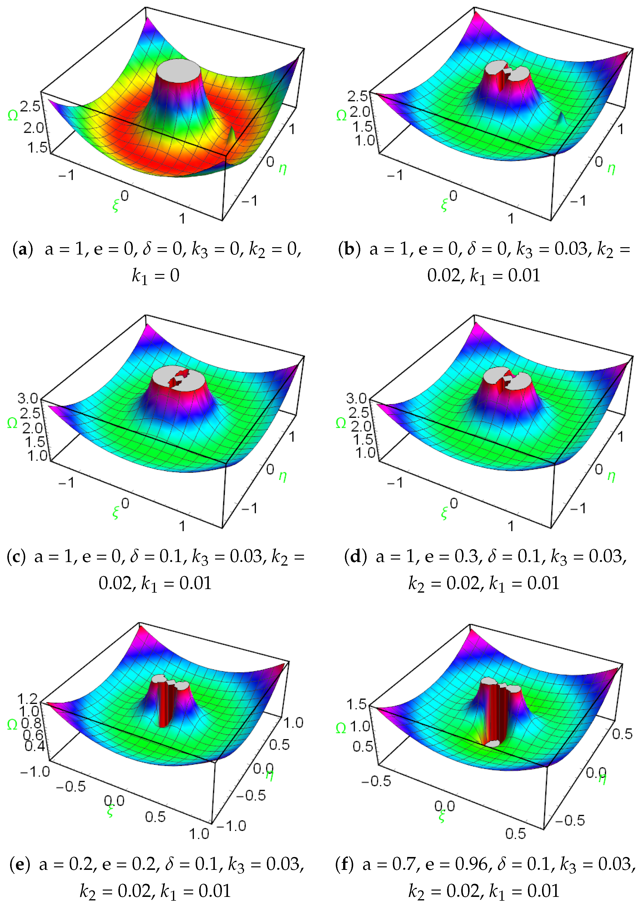
The potential surfaces have been drawn with the use of Equation (2) for the six different cases with the use of the stated parameters. These graphs are given in Figure 2a–f. Figure 2a represents the classical circular restricted three-body problem. We can observe here that both primaries are visible as two poles. Simultaneously, it can also be observed that the potential surface increases where the color shows the different stages of variations. Next, Figure 2b represents the effect of heterogeneous density of the primary; here also two poles are visible, but due to heterogeneity, the shape of the first pole is divided into two parts. Further, Figure 2c,d and Figure 2e,f represent the modified Newtonian effect and the elliptic cases, respectively, where we observe that only one pole in three parts appears. We also observe that when the modified Newtonian effect is considered, the surfaces expand, while when the semi-major axis (a) decreases, the surfaces shrink. In this way, the potential surfaces are affected by these parameters.

5.2. Locations of Equilibrium Points

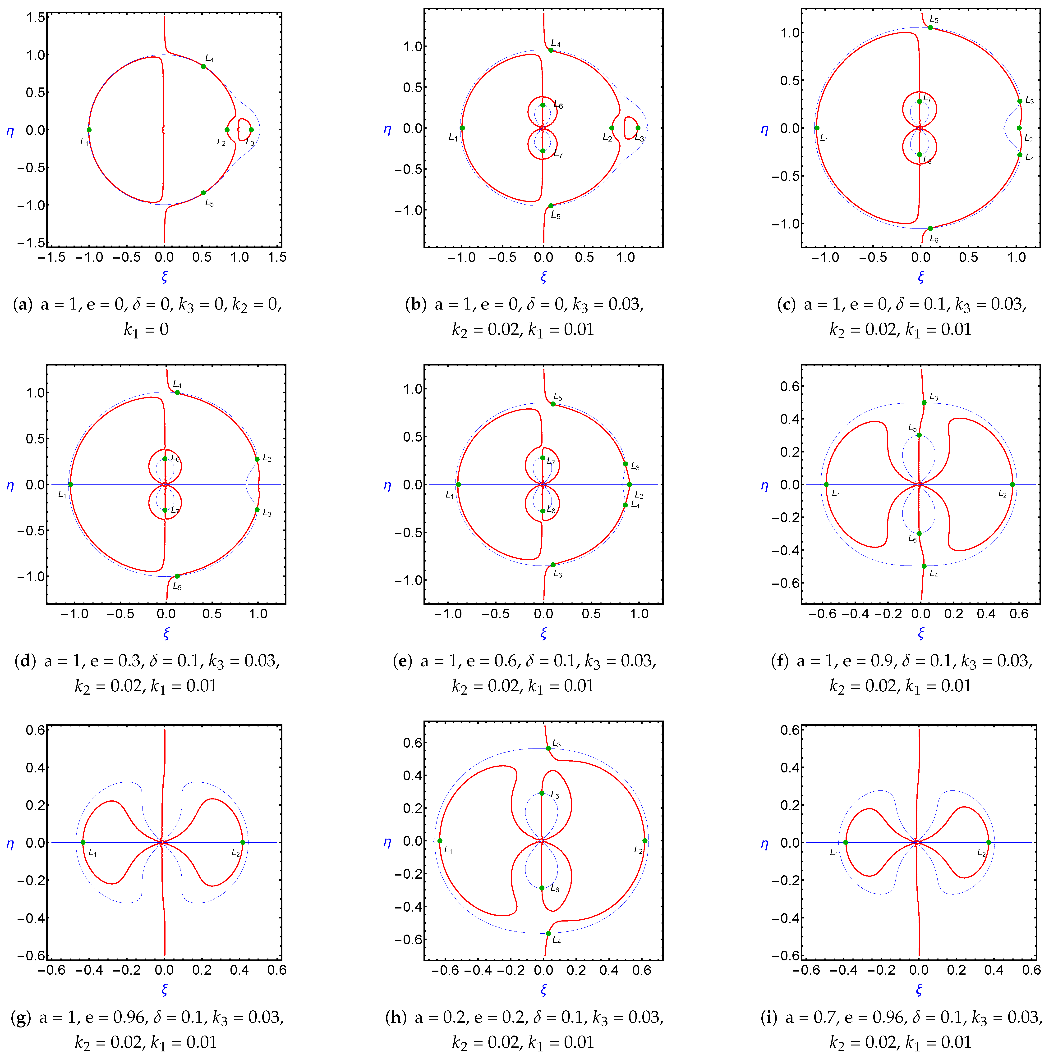
In-plane locations of equilibrium points can be plotted by solving the equations ${\displaystyle {\mathsf{\Omega }}_{\xi }=0}$ and ${\displaystyle {\mathsf{\Omega }}_{\eta }=0}$ obtained from (1) with ${\displaystyle \zeta =0}$. We have plotted numerically equilibrium points in nine cases for various values of the stated parameters. We have found a maximum of eight equilibrium points and a minimum of two equilibrium points in this case. These graphs are given in Figure 3a–i. Figure 3a represents the graph for the classical circular restricted three-body problem where we obtain the five well-known equilibrium points. Figure 3b represents the graph for the homogeneous effect where we obtain seven equilibrium points, out of which three are collinear and four are non-collinear equilibrium points.

Figure 3c represents the modified Newtonian effect where we obtain eight equilibrium points, out of which two are collinear and six are non-collinear equilibrium points. Figure 3d, Figure 3e, Figure 3f and Figure 3g represent the changes in eccentricity (0.3, 0.6, 0.9 and 0.96) where we obtain seven, eight, six, and two equilibrium points, respectively, out of which one is on the ${\displaystyle \xi }$-axis and six are non-collinear equilibrium points. The effects of the semi-major axis are shown in Figure 3h and Figure 3i, where we obtain six and two equilibrium points, respectively. This shows that these parameters have great impact on the locations of equilibrium points.

5.3. Regions of Motion

Multiplying the first, second, and third equations of system (1) by ${\displaystyle \xi }$, ${\displaystyle {\eta }^{\prime }}$, and ${\displaystyle {\zeta }^{\prime }}$, respectively, and then integrating their sum, we obtain

$$\begin{array}{ccc}{\xi }^{\prime 2}+{\eta }^{\prime 2}+{\zeta }^{\prime 2}\hfill & =& 2\mathsf{\Omega }-C.\hfill \end{array}$$

(31)

where C is a constant known as the Jacobian constant. Equation (31) is called the Jacobian integral. Its left-hand side represents the square of the velocity (${\displaystyle v^2}$) of the infinitesimal body.

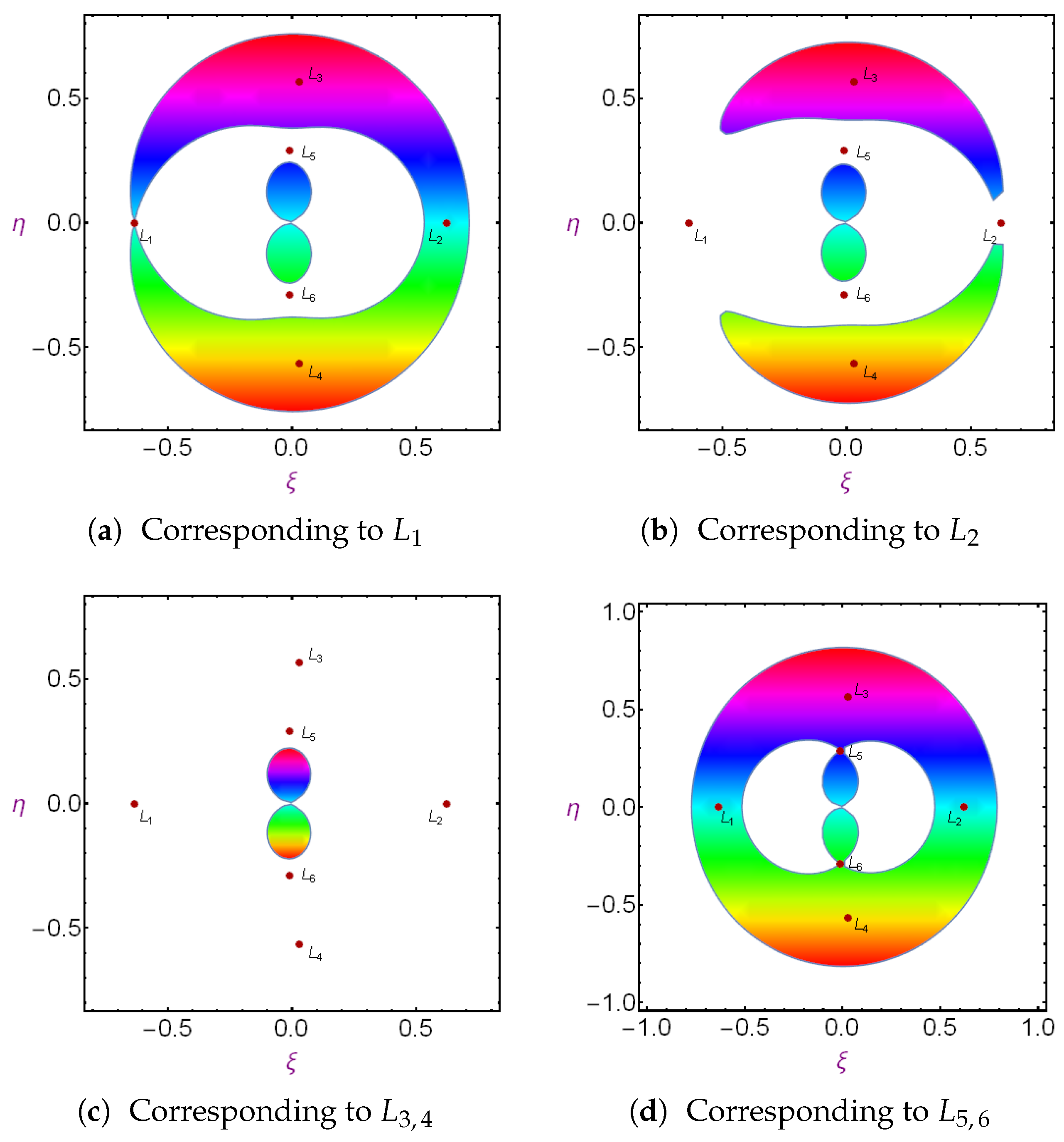
Regions of motions are illustrated corresponding to equilibrium points with the aid of Mathematica. To do so, the velocity vs. can be taken as zero. Therefore, from Equation (31), we obtain ${\displaystyle 2\mathsf{\Omega }=C}$. From here, firstly, we have to find the value of the Jacobian constant ${\displaystyle C}$ corresponding to each equilibrium point. Then, by the potential function ${\displaystyle \mathsf{\Omega }}$, the evaluated value of ${\displaystyle C}$ and the Region-plot, we shall illustrate the regions of motion.

Here, we have plotted the regions of motion for the equilibrium points obtained in Figure 3h, i.e., corresponding to the equilibrium points ${\displaystyle L_{1,2,3,4,5,6}}$ for a = 0.2, e = 0.2, ${\displaystyle \delta }$ = 0.1, ${\displaystyle k_3}$ = 0.03, ${\displaystyle k_2}$ = 0.02, and ${\displaystyle k_1}$ = 0.01. These graphs of regions of motion are given in Figure 4a, Figure 4b, Figure 4c and Figure 4d, which correspond to the equilibrium points ${\displaystyle L_1}$, ${\displaystyle L_2}$, ${\displaystyle L_{3,4}}$, and ${\displaystyle L_{5,6}}$, respectively. In these figures, the color regions are prohibited regions, while the white regions are allowed regions for motion.

5.4. Periodic Orbits

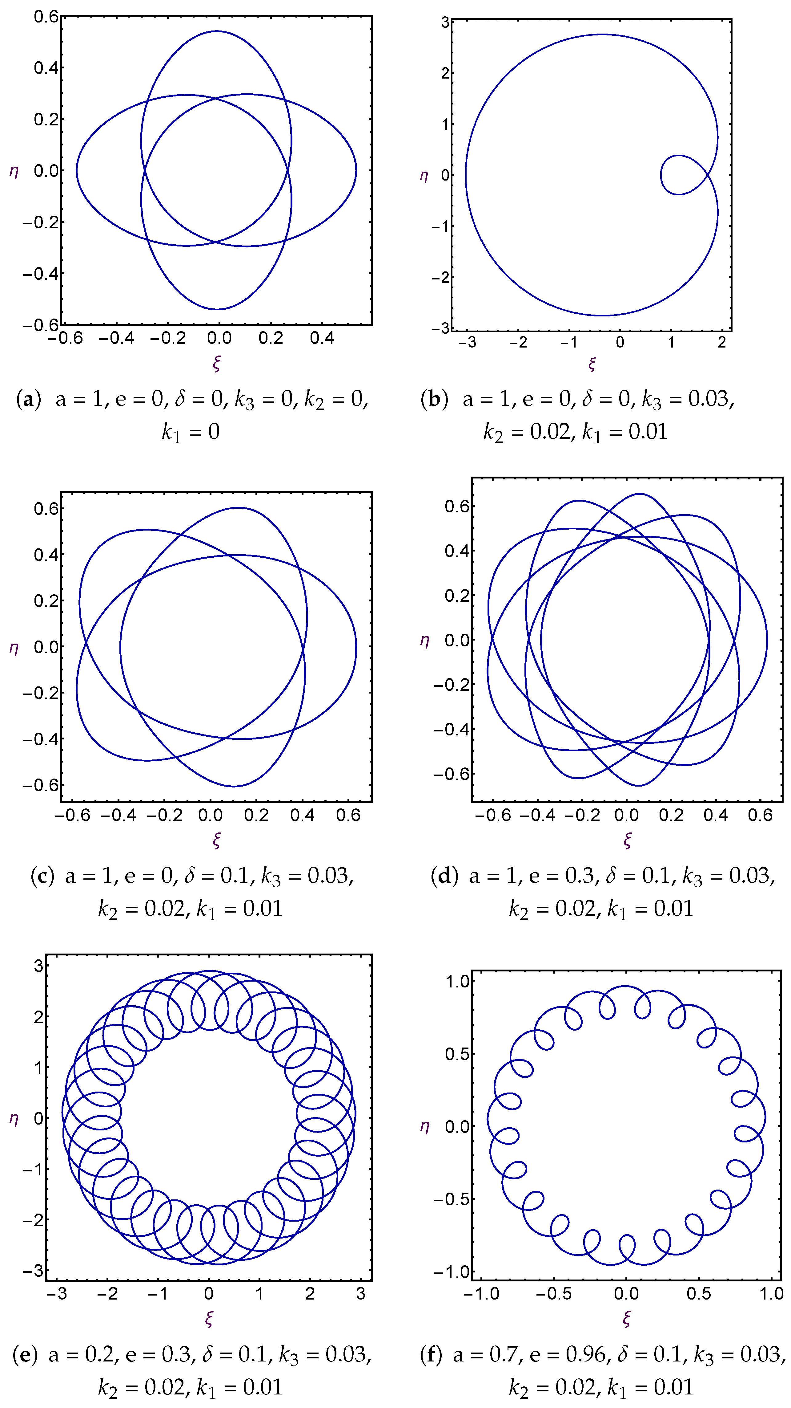
Periodic orbits can be illustrated with the help of Equation (1) for which, firstly, we need to transform the equations of motion into phase space and then with the proper choices of initial values, we solve the phase-space equations from where we obtain the positions and velocities of the infinitesimal body. If we plot the graph between abscissa and ordinates with the proper choices of the initial values, we obtain the periodic orbits. For our model, also, we have plotted the periodic orbits in six cases. These graphs are given in Figure 5a, Figure 5b, Figure 5c, Figure 5d, Figure 5e and Figure 5f with the time-periods 6.32, 10.6, 9.95, 20.1, 48.815, and 16.27 units, respectively.

5.5. Basins of Attracting Domain

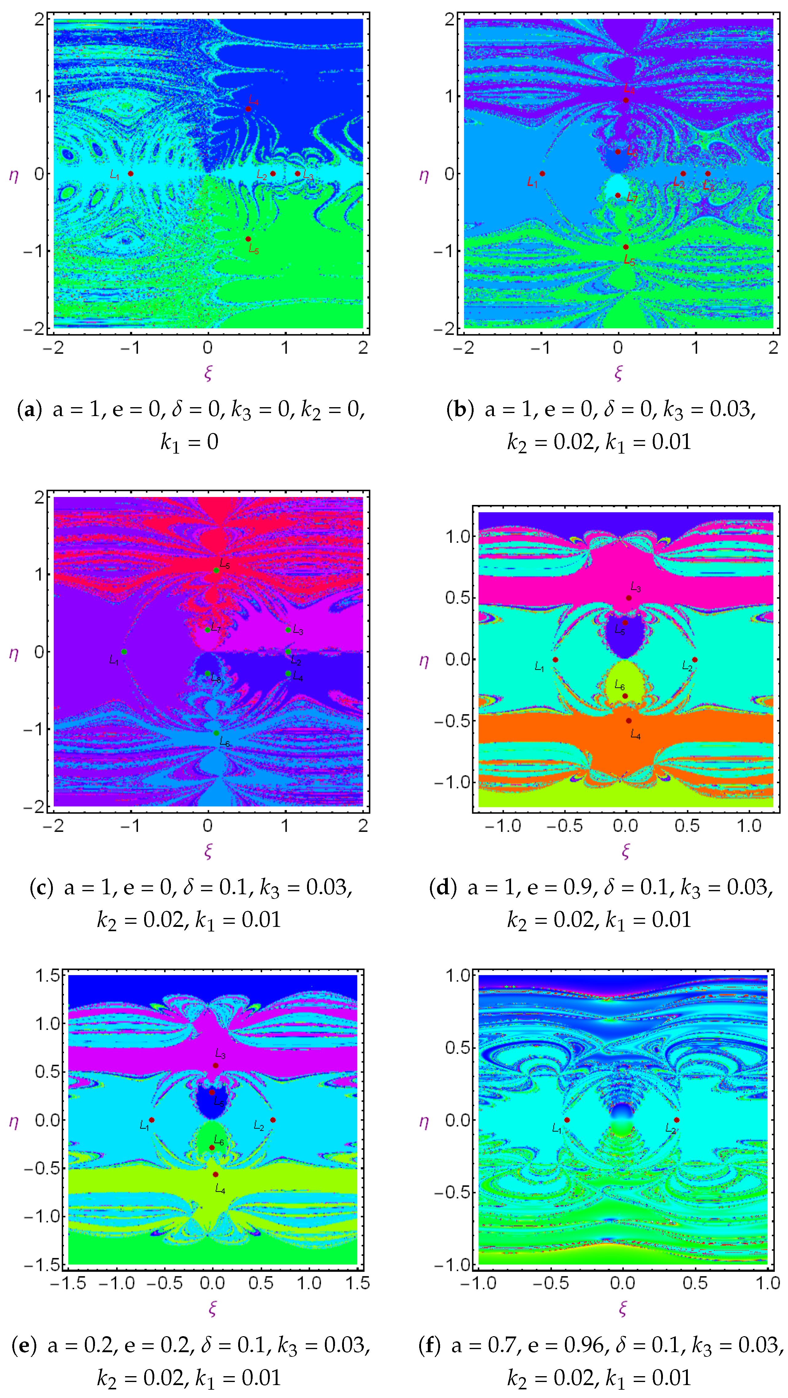
Basins of attraction can be illustrated by utilizing the method given by [33]. The authors used the N-R iterative method, which is easy and simpler than the other methods. The algorithm for this method is as follows:

$$\left\{\begin{array}{ccc}{\xi }_{n+1}\hfill & =& {\xi }_n-{\left({\displaystyle \frac{{\mathsf{\Omega }}_{\xi }{\mathsf{\Omega }}_{\eta \eta }-{\mathsf{\Omega }}_{\eta }{\mathsf{\Omega }}_{\xi \eta }}{{\mathsf{\Omega }}_{\xi \xi }{\mathsf{\Omega }}_{\eta \eta }-{\mathsf{\Omega }}_{\xi \eta }{\mathsf{\Omega }}_{\eta \xi }}}\right)}_{\left({\xi }_n{\eta }_n\right)},\hfill \\ {\eta }_{n+1}\hfill & =& {\eta }_n-{\left({\displaystyle \frac{{\mathsf{\Omega }}_{\eta }{\mathsf{\Omega }}_{\xi \xi }-{\mathsf{\Omega }}_{\xi }{\mathsf{\Omega }}_{\eta \xi }}{{\mathsf{\Omega }}_{\xi \xi }{\mathsf{\Omega }}_{\eta \eta }-{\mathsf{\Omega }}_{\xi \xi }{\mathsf{\Omega }}_{\eta \xi }}}\right)}_{\left({\xi }_n{\eta }_n\right)},\hfill \end{array}\right.$$

(32)

where ${\displaystyle {\xi }_n}$ and ${\displaystyle {\eta }_n}$ are the values of ${\displaystyle \xi }$ and ${\displaystyle \eta }$ at the ${\displaystyle n}$-th step of the N-R iterative method.

Here, the basins of attraction are drawn with the use of a suitable number of iterations in Mathematica and the formulae given in Equation (32) for six cases and these are given in Figure 6a–f. The color code is used for observing the various regions. In these cases, we observe that all the corresponding attracting regions are extended to infinity.

5.6. Linear Stability of the Equilibrium Points

We have numerically evaluated the roots of Equation (30). For the equilibrium points obtained in Figure 3a, Figure 3e and Figure 3h, these roots are tabulated in

Table 1. The nature of roots corresponding to Figure 3a.

${\displaystyle \mathit{Equilibrium}\mathit{Points}(\mathit{\xi },\mathit{\eta })}$	${\displaystyle \mathit{Roots}}$	${\displaystyle \mathit{Nature}}$
${\displaystyle L_1(-1.00000,0.00000)}$	${\displaystyle -0.2764792657,\mathbf{0.2764792657}}$${\displaystyle 0.0000000000\pm 1.0247652721i}$	${\displaystyle Unstable}$
${\displaystyle L_2(0.83500,0.00000)}$	${\displaystyle -2.8905571465,\mathbf{2.8905571465}}$${\displaystyle 0.0000000000\pm 2.3082731898i}$	${\displaystyle Unstable}$
${\displaystyle L_3(1.15700,0.00000)}$	${\displaystyle -2.1295583381,\mathbf{2.1295583381}}$${\displaystyle 0.0000000000\pm 1.8456402052i}$	${\displaystyle Unstable}$
${\displaystyle L_{45}(0.52000,0.84000)}$	${\displaystyle 0.0000000000\pm 0.2053180000i}$${\displaystyle 0.0000000000\pm 0.9692620000i}$	${\displaystyle Stable}$

,

Table 2. The nature of roots corresponding to Figure 3e.

${\displaystyle \mathit{Equilibrium}\mathit{Points}(\mathit{\xi },\mathit{\eta })}$	${\displaystyle \mathit{Roots}}$	${\displaystyle \mathit{Nature}}$
${\displaystyle L_1(-0.89000,0.00000)}$	${\displaystyle -0.7992986560,\mathbf{0.7992986560}}$${\displaystyle 0.0000000000\pm 0.9448512765i}$	${\displaystyle Unstable}$
${\displaystyle L_2(0.90000,0.00000)}$	${\displaystyle -0.9538175435\pm 0.9180815619i}$${\displaystyle \mathbf{0.9538175435}\pm 0.9180815619i}$	${\displaystyle Unstable}$
${\displaystyle L_{3,4}(0.85700\pm 0.21500)}$	${\displaystyle -0.9084650000,\mathbf{0.9084650000}}$${\displaystyle 0.1000000000\pm 1.1812100000i}$	${\displaystyle Unstable}$
${\displaystyle L_{5,6}(0.109600\pm 0.84000)}$	${\displaystyle -0.4424408390\pm 0.6325145473i}$${\displaystyle \mathbf{0.4424408390}\pm 0.6325145473i}$	Unstable
${\displaystyle L_{7,8}(-0.01000\pm 0.27840)}$	${\displaystyle -5.5214418905,\mathbf{5.5214418905}}$${\displaystyle 0.0000000000\pm 8.82925733i}$	${\displaystyle Unstable}$

and

Table 3. The nature of roots corresponding to Figure 3h.

${\displaystyle \mathit{Equilibrium}\mathit{Points}(\mathit{\xi },\mathit{\eta })}$	${\displaystyle \mathit{Roots}}$	${\displaystyle \mathit{Nature}}$
${\displaystyle L_1(-0.63250,0.000)}$	${\displaystyle -0.6502440000,\mathbf{0.6502440000}}$${\displaystyle 0.0000000000\pm 1.1886400000i}$	${\displaystyle Unstable}$
${\displaystyle L_2(0.61900,0.00000)}$	${\displaystyle -0.5296750039,\mathbf{0.5296750039}}$${\displaystyle 0.0000000000\pm 1.1623551235i}$	${\displaystyle Unstable}$
${\displaystyle L_{3,4}(0.03000,0.56500)}$	${\displaystyle -0.2515419544\pm 0.8503778010i}$${\displaystyle \mathbf{0.2515419544}\pm 0.8503778010i}$	${\displaystyle Unstable}$
${\displaystyle L_{5,6}(0.01000,0.28900)}$	${\displaystyle -2.4920000000,\mathbf{2.4920000000}}$${\displaystyle 0.0000000000\pm 4.2583000000i}$	${\displaystyle Unstable}$

, respectively. From these tables, we can observe that out of four roots, at least one is a positive real root or positive real part of a complex root, which are highlighted as bold in the tables. Hence, these equilibrium points are unstable except the non-collinear equilibrium points for Figure 3a. In this way, we can tabulate the other values for the stated parameters.

6. Conclusions and Discussion

Considering a heterogeneous triaxial rigid body as the primary and a spherical rigid body subjected to a modified Newtonian potential as the secondary, we have investigated the motion of an infinitesimal body within the framework of the elliptic restricted three-body problem. The analysis demonstrates that the dynamical characteristics of the system are significantly influenced by the physical and orbital parameters involved.

It is observed that the number of equilibrium points obtained analytically does not always agree with the number identified through numerical investigations. This discrepancy may be attributed to the use of a tolerable first-order approximation in the analytical treatment, whereas the numerical analysis accounts for even very small values of the system parameters. The stability analysis further reveals that the non-collinear equilibrium points are stable for (${\displaystyle 0<\mu <{\mu }_c}$) and become unstable for (${\displaystyle {\mu }_c\le \mu \le \frac{1}{2}}$), where (${\displaystyle {\mu }_c}$) denotes the critical mass ratio, which depends on the parameters of the system. In contrast, all the collinear equilibrium points are found to be unstable for the entire range of the mass ratio.

Numerical investigations have also been carried out to examine the effects of the system parameters on the potential surfaces, locations of equilibrium points, permissible regions of motion, periodic orbits, basins of attraction, and linear stability of the equilibrium points. The potential surfaces indicate that the inclusion of the modified Newtonian effect causes the surfaces to expand, whereas a decrease in the semi-major axis results in their contraction. Furthermore, the numerical analysis reveals the existence of a maximum of eight and a minimum of two equilibrium points, depending on the values of the system parameters. This result differs significantly from the classical restricted three-body problem, in which only five equilibrium points are generally obtained.

The regions of motion are also investigated, where the colored regions represent prohibited regions and the white regions correspond to the permissible regions in which the infinitesimal body can move. The numerical simulations demonstrate the existence of periodic orbits with different time periods, whose characteristics vary with the system parameters. In addition, the basins of attraction are examined for different parameter values. The results show the presence of distinct attraction regions, which are extend to infinity. Finally, the linear stability analysis indicates that all the equilibrium points are unstable except for certain triangular equilibrium points, which may remain stable within specific ranges of the mass ratio and other system parameters. Overall, the results provide a comprehensive understanding of the influence of the modified gravitational potential, triaxiality, and mass heterogeneity on the dynamics of the elliptic restricted three-body problem. The findings may be useful for researchers working in celestial mechanics, dynamical astronomy, and related areas involving the motion and stability of celestial bodies.

References

1. Szebehely, V. Theory of Orbits; Academic Press: New York, NY, USA, 1967. [Google Scholar]
2. Henon, M. Numerical exploration of the restricted problem. Hill’s case: Periodic orbits and their stability. Astron. Astrophy 1969, 1, 223–238. [Google Scholar]
3. Sharma, R.K.; Subba Rao, P.V. Stationary solutions and their characteristic exponents in the restricted three-body problem when the more massive primary is an oblate spheroid. Celest. Mech. 1976, 13, 137–149. [Google Scholar] [CrossRef] [Scilit]
4. Gyorgyey, J. On the non-linear stability of motions around L5 in the elliptic restricted three bodies. Celest. Mech. 1985, 36, 281–285. [Google Scholar] [CrossRef] [Scilit]
5. Ragos, O.; Zagouras, C. Periodic solutions about the out-of-plane equilibrium points in the photogravitational restricted three-body problem. Celest. Mech. 1988, 44, 135–154. [Google Scholar] [CrossRef] [Scilit]
6. Kumar, V.; Choudhary, R.K. Linear stability and the resonance cases for the triangular libration points for the doubly photo-gravitational elliptic restricted problem of three bodies. Celest. Mech. Dyn. Astron. 1989, 46, 59–77. [Google Scholar] [CrossRef] [Scilit]
7. Zagouras, C.G. Periodic motion around the triangular equilibrium points of the photogravitational restricted problem of three bodies. Celest. Mech. Dyn. Astron. 1991, 51, 331–348. [Google Scholar] [CrossRef] [Scilit]
8. Dvorak, R. Progress in the elliptic restricted 3-body problem: Asteroids in the 2/1, 3/1 and 1/1 resonance. Celest. Mech. Dyn. Astron. 1992, 54, 195–205. [Google Scholar] [CrossRef] [Scilit]
9. Hadjidemetriou, J.D. The elliptic restricted problem at the 3:1 resonance. Celest. Mech. Dyn. Astron. 1992, 53, 151–183. [Google Scholar] [CrossRef] [Scilit]
10. Murray, C.D.; Dermott, S.F. Solar System Dynamics; Cambridge University Press: Cambridge, UK, 1999. [Google Scholar]
11. Sharma, R.K.; Taqvi, Z.A.; Bhatnagar, K.B. Existence and stability of libration points in the restricted three-body problem when the primaries are triaxial rigid bodies. Celest. Mech. Dyn. Astron. 2001, 79, 119–133. [Google Scholar] [CrossRef] [Scilit]
12. Esteban, E.P.; Vazquez, S. Rotating stratifield heterogeneous oblate spheroid in newtonian physics. Celest. Mech. Dyn. Astron. 2001, 81, 299–312. [Google Scholar] [CrossRef] [Scilit]
13. Zimovshchikov, A.S.; Tkhai, V.N. Instability of libration points and resonance phenomena in the photogravitational elliptic restricted three-body problem. Sol. Syst. Res. 2004, 38, 155–164. [Google Scholar] [CrossRef] [Scilit]
14. Tsirogiannis, G.A.; Douskos, C.N.; Perdios, E.A. Computation of the liapunov orbits in the photogravitational rtbp with oblateness. Astrophys. Space Sci. 2006, 305, 389–398. [Google Scholar] [CrossRef] [Scilit]
15. Vishnu Namboodiri, N.I.; Sudheer Reddy, D.; Sharma, R.K. Effect of oblateness and radiation pressure on angular frequencies at collinear points. Astrophys. Space Sci. 2008, 318, 161–168. [Google Scholar] [CrossRef] [Scilit]
16. Abdulraheem, A.; Singh, J. Combined effects of perturbations, radiation and oblateness on the periodic orbits in the restricted three-body problem. Astrophys. Space Sci. 2008, 317, 9–13. [Google Scholar] [CrossRef] [Scilit]
17. Ershkov, S.V. The yarkovsky effect in generalized photogravitational 3-body problem. Planet. Space Sci. 2021, 73, 221–223. [Google Scholar] [CrossRef] [Scilit]
18. Ershkov, S.V. Stability of the moons orbits in solar system in the restricted three-body problem. Adv. Astron. 2015, 97, 615029. [Google Scholar] [CrossRef] [Scilit]
19. Safiya Beevi, A.; Sharma, R.K. Oblateness effects of saturn on periodic orbits in the saturn-titan restricted three-body problem. Astrophys. Space Sci. 2012, 340, 245–261. [Google Scholar] [CrossRef] [Scilit]
20. Abouelmagd, E.I.; Asiri, H.M.; Sharaf, M.A. The effect of oblateness in the perturbed restricted three-body problem. Meccanica 2013, 48, 2479–2490. [Google Scholar] [CrossRef] [Scilit]
21. Mia, R. Lie-series solution of the restricted three-body problem: Application to binary stellar system. J. Astronaut. Sci. 2020, 67, 59–76. [Google Scholar] [CrossRef] [Scilit]
22. Ansari, A.A. Heterogeneous primary in the restricted three-body problem with modified Newtonian potential of secondary. Bulg. Astron. J. 2021, 35, 76. [Google Scholar]
23. Abouelmagd, E.I.; Pal, A.K.; Guirao, J.L.G. Analysis of nominal halo orbits in the sun–earth system. Arch. Appl. Mech. 2021, 91, 4751–4763. [Google Scholar] [CrossRef] [Scilit]
24. Pal, A.K.; Abouelmagd, E.I.; Kishor, R. Effect of moon perturbation on the energy curves and equilibrium points in the sun–earth–moon system. New Astron. 2021, 84, 101505. [Google Scholar] [CrossRef] [Scilit]
25. Albidah, A.B.; Abdullah, A.A. Shapes and mass variation effects of the bodies in the generalized elliptic restricted 3-body problem. Astron. Rep. 2023, 67, 393–403. [Google Scholar] [CrossRef] [Scilit]
26. Mia, R.; Prasadu, B.R.; Abouelmagd, E.I. Analysis of stability of non-collinear equilibrium points: Application to sun–mars and proxima centauri systems. Acta Astronaut. 2023, 204, 199–206. [Google Scholar] [CrossRef] [Scilit]
27. Vincent, A.E.; Abouelmagd, E.I.; Perdios, E.A.; Kalantonis, V.S. Numerical exploration of the quantized hill problem dynamics. Chaos Solitons Fractals 2024, 181, 114688. [Google Scholar] [CrossRef] [Scilit]
28. Yadav, P.; Abdullah; Prasad, S.N. New kind of perturbed robe’s problem with heterogeneous body and kerr-like secondary. Mod. Phys. Lett. A 2025, 28, 2550184. [Google Scholar] [CrossRef] [Scilit]
29. Singh, J.; Umar, A. Motion in the photogravitational elliptic restricted three-body problem under an oblate primary. Astron. J. 2012, 143, 109. [Google Scholar] [CrossRef] [Scilit]
30. Ansari, A.A.; Shalini, K.; Alhussain, Z.A. Non-linear stability of L4 in the r3bp when the smaller primary is a heterogeneous triaxial rigid body with n-layers. Ital. J. Pure Appl. Math. 2019, 41, 297–312. [Google Scholar]
31. Abouelmagd, E.I. Periodic solution of the two-body problem by kb averaging method within frame of the modified newtonian potential. J. Astronaut. Sci. 2018, 65, 291–306. [Google Scholar] [CrossRef] [Scilit]
32. Ansari, A.A.; Abouelmagd, E.I. Gravitational potential formulae between two bodies with fnite dimensions. Astron. Nachrichten 2020, 341, 656–668. [Google Scholar] [CrossRef] [Scilit]
33. Abouelmagd, E.I.; Ansari, A.A. The motion properties of the infinitesimal body in the framework of bicircular Sun perturbed Earth-Moon system. New Astron. 2019, 73, 101282. [Google Scholar] [CrossRef] [Scilit]
Figure 1. Geometric configuration of the problem.
Symmetry 18 01494 g001
Figure 2. Potential surfaces for different cases.
Symmetry 18 01494 g002
Figure 3. Equilibrium point positions for different cases.
Symmetry 18 01494 g003
Figure 4. Regions of motion for a = 0.2, e = 0.2, δ = 0.1, k 3 = 0.03, k 2 = 0.02, and k 1 = 0.01.
Symmetry 18 01494 g004
Figure 5. Periodic orbits for different cases.
Symmetry 18 01494 g005
Figure 6. Basins of attraction for different cases.
Symmetry 18 01494 g006