Calibration and Evaluation of an IMK Hysteretic Model for Seismic Fragility Assessment of Urban Rail RC Solid Piers

Abstract

Rapid post-earthquake assessment of urban rail viaducts requires nonlinear pier models that capture cyclic deterioration at manageable computational costs. This study calibrates and evaluates the established Ibarra–Medina–Krawinkler (IMK) formulation for reinforced-concrete solid piers rather than proposing a new hysteretic law or experimental database. Seven previously reported quarter-scale tests are reused for direction-specific parameter identification and calibration-set assessment. The new contribution is a multilevel accuracy–efficiency evaluation covering cyclic metrics, a scaled 12 m Fiber benchmark, nonlinear dynamics, incremental dynamic analysis (IDA), computational cost, and fragility. For the specimens, final secant stiffness achieved R² = 0.891 and a 9.93% mean absolute percentage error; cumulative energy achieved R² = 0.893 but a 27.79% error. For the prototype, the intermediate-backbone force difference was 3.83%. Under eight representative records, mean differences were 2.64% for peak base shear and 4.15% for peak displacement. Across 60 records scaled from PGA = 0.1 to 1.5 g, peak–displacement and peak–base–shear comparisons yielded R² values of 0.854 and 0.931. The corresponding mean absolute percentage errors were 15.95% and 11.32%. The IMK model reduced wall-clock time by 96.37%, a 27.55-fold speed-up. Paired fragility curves differed by 3.14 percentage points on average, and median PGA capacities differed by 11.23%; Sa(T1) and capacity-dispersion checks preserved the main comparison. Because the record groups were not matched in spectral amplitude or velocity, their ranking is interpreted as an association rather than a causal pulse-period effect. The calibrated IMK model is therefore suitable for rapid global demand and fragility assessment within its calibration domain, whereas Fiber models remain preferable for local damage, residual deformation, and detailed energy dissipation.

1. Introduction

Urban rail transit supports mobility, emergency access, and economic recovery in dense cities. Post-earthquake functionality depends on structural condition and recovery coordination [1], nonstructural interactions [2], source-to-structure effects [3], and network accessibility [4]. Rapid viaduct-pier assessment is therefore essential for inspection, traffic control, and recovery planning.

Earthquake damage can propagate through piers, fasteners, track-bridge interfaces, and other operational components. Rail-fastener response affects viaduct demand [5], component damage sequences influence failure progression [6], and accumulated track-bridge damage can reduce running safety [7]. System-wide mitigation is consequently important [8]. At the pier level, long-duration and near-fault motions modify deformation and failure probability [9]. Tests link column response to system behavior [10], while geometry and reinforcement [11], flexure–shear coupling [12], and damage localization [13] govern failure progression. Pier response is therefore central to rapid seismic damage estimation.

Fragility analysis converts nonlinear response into damage-state exceedance probabilities for retrofit and emergency decisions. Mechanics-based models address shear-dominant piers [14], while pulse-like motions and axial load affect performance [15]. Railway and experimental studies extend fragility assessment to double-column systems [16] and variable axial loads [17]. Risk-targeted formulations connect damage probabilities with design objectives [18], near-fault studies quantify record effects [19], and residual-demand models support resilience assessment [20].

Recent work extends fragility to deterioration [21], climate-related corrosion [22], bridge portfolios [23], catenary systems [24], and resilience-restoration coupling [25]. These applications require many nonlinear analyses, making repeated high-fidelity simulation costly. Machine learning response predictors [26], data-driven fragility equations [27], efficient intensity measures [28], neural-network damping estimates [29], and stiffness predictors [30] can reduce cost. However, surrogate methods require representative training data and may not preserve cyclic mechanisms outside their calibration domain.

Physics-based simplified hysteretic models provide a complementary way to reduce each nonlinear analysis. The established IMK formulation represents backbone response, residual strength, pinching, and energy-based cyclic deterioration [31,32]. For urban rail RC solid piers, the unresolved need is not a new formulation but transparent calibration and multilevel accuracy–efficiency evaluation spanning cyclic response, full-scale extrapolation, IDA, and fragility.

Accordingly, the IMK and Fiber representations are compared at the specimen, 12 m analytical-prototype, and system-fragility levels. Independent positive- and negative-direction parameters quantify the observed departure from symmetric hysteresis and test whether the simplified model preserves this asymmetry globally. This study reports response error, computational acceleration, fragility differences, and applicability limits within the investigated calibration domain.

2. Numerical Modeling Framework

2.1. Simplified IMK Concentrated-Plasticity Model

The Ibarra–Medina–Krawinkler (IMK) hysteretic model can represent pinching and cyclic deterioration of structural components [31,32]. Its principal components, including the backbone curve, pinching rule, and energy-based deterioration rules, are described below.

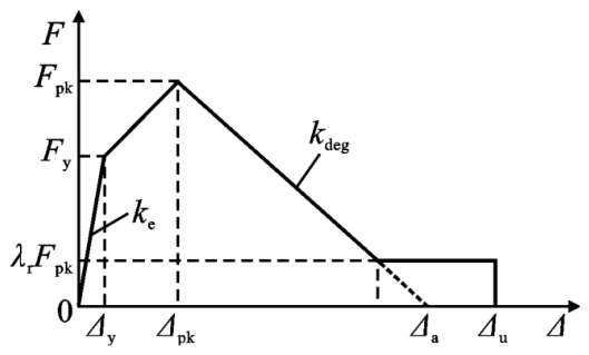
The backbone curve of the IMK model is shown in Figure 1. Before post-capping softening occurs, it is defined by the elastic stiffness $k_e$, yield strength $F_y$, and post-yield stiffness $k_s$, as follows:

$$k_s={\alpha }_s{k}_e$$

(1)

where ${\alpha }_s$ is the post-yield stiffness ratio. The response increases from the yield point ${(\mathsf{\Delta }}_y)$ to the peak point ${(\Delta }_{pk}{,F}_{pk})$. Thereafter, the strength decreases along the post-capping branch, whose negative stiffness is expressed as

$$k_c={\alpha }_c{k}_e$$

(2)

where ${\alpha }_{c<0}$ is the post-capping stiffness ratio.

After the strength decreases to the residual value, it remains constant until the ultimate deformation ${\Delta }_u$ is reached. To maintain a single notation throughout this study, the residual strength is defined relative to the yield strength as

$$F_r=k_{ry}{F}_y$$

(3)

where k_ry = F_r/F_y is the residual-to-yield strength ratio. The related peak-to-yield strength ratio is k_py = F_pk/F_y. Both ratios and the remaining backbone parameters can be defined independently in the positive and negative loading directions, allowing directional asymmetry to be represented explicitly.

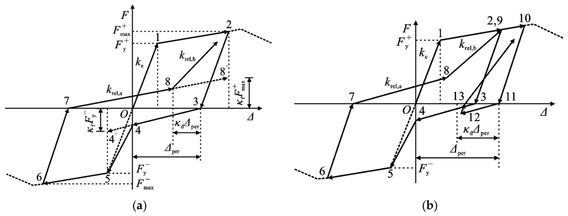
The pinching rule of the IMK model is illustrated in Figure 2. As shown in Figure 2a, the reloading path is generally divided into two branches. The first branch extends from the unloading-completion point to the pinching control point with reloading stiffness $k_{rel,a}$. The second branch extends from the pinching point toward the maximum deformation previously attained in the same loading direction with stiffness $k_{rel,b}$.

The pinching-point location is controlled by the force parameter ${kappa}_F$ and deformation parameter ${kappa}_D$. These parameters govern the severity of pinching and the enclosed hysteresis-loop area. As shown in Figure 2b, if reloading begins beyond the pinching-control deformation, the response reloads directly toward the previously attained maximum-deformation point.

The cyclic deterioration rules of the IMK model follow the energy-dependent formulation developed by Rahnama and Krawinkler [31,33]. The deterioration parameter for the ith inelastic excursion and deterioration mode m is defined as

$${\beta }_i={\left({\displaystyle \frac{E_i}{E_t-{\displaystyle {\sum }_{j=1}^i}{E}_j}}\right)}^c$$

(4)

where $E_i$ is the hysteretic energy dissipated during the $i$th excursion, $\sum E_j$ is the energy dissipated during the preceding excursions, $E_{t,m}$ is the reference energy capacity, and $c$ controls the deterioration rate. The subscript $m$ represents the corresponding deterioration mode.

The reference energy capacity for mode m is expressed as

$$E_t=\gamma F_y{\mathsf{\Delta }}_y$$

(5)

where $\gamma$ is a parameter used to calibrate the energy dissipation capacity of the component.

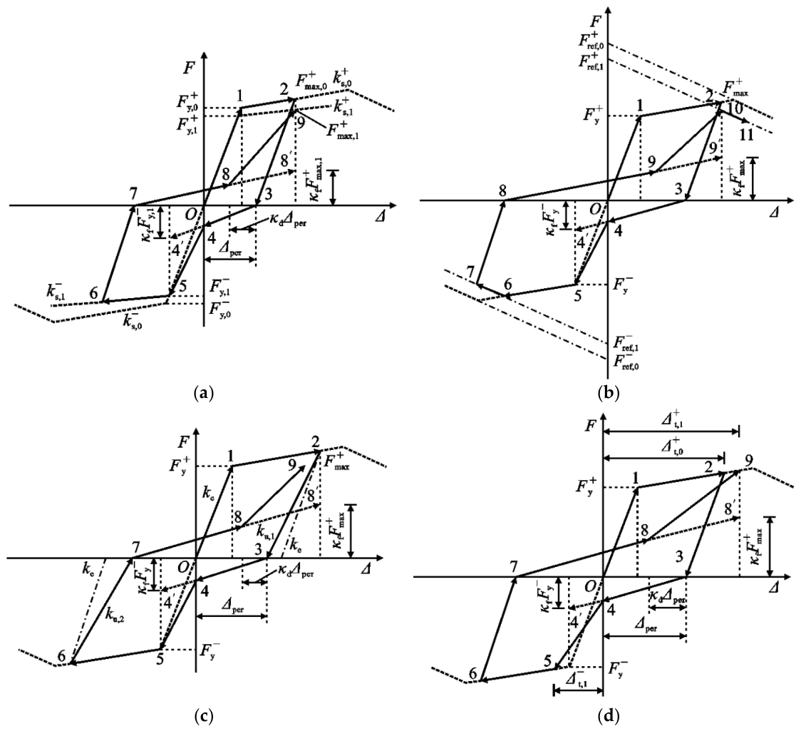
After reinforced concrete members exceed the yield point, their hysteretic behavior can deteriorate through four mechanisms, as shown in Figure 3 [31,34]: basic strength deterioration, post-capping strength deterioration, unloading stiffness deterioration, and accelerated reloading deterioration.

The deterioration of the basic strength includes the deterioration of both the yield strength $F_y$ and the hardening stiffness $K_s$. The yield strength $F_y$ is expressed as

$$\left\{\begin{array}{c}{F}_{y,i}^{+}={\left(1-{\beta }_{s,i}\right)F}_{y,i-1}^{+}\\ F_{y,i}^{-}={\left(1-{\beta }_{s,i}\right)F}_{y,i-1}^{-}\end{array}\right.$$

(6)

where $F_{y,i}^{+}$ and $F_{y,i}^{-}$ are the yield strengths in the positive and negative loading directions, respectively, for the $i$th loading cycle considering deterioration; ${\beta }_{s,i}$ is the deterioration parameter ${\beta }_i$ corresponding to the basic strength deterioration and is calculated using Equation (4). In this calculation, $E_t$ is expressed in terms of ${\gamma }_s$ according to Equation (5), where ${\gamma }_s$ denotes the parameter $\gamma$ associated with basic strength deterioration.

The hardening stiffness $k_s$ is the stiffness of the hardening branch between the yield strength and the peak strength, and its deterioration can be expressed as

$$\left\{\begin{array}{c}{k}_{s,i}^{+}={\left(1-{\beta }_{s,i}\right)k}_{s,i-1}^{+}\\ k_{s,i}^{-}={\left(1-{\beta }_{s,i}\right)k}_{s,i-1}^{-}\end{array}\right.$$

(7)

where $k_{s,i}^{+}$ and $k_{s,i}^{-}$ are the hardening stiffnesses in the positive and negative loading directions, respectively, for the $i$ th loading cycle considering deterioration.

It should be noted that, as shown in Figure 3a, Point 8 depends on the lateral force corresponding to Point 9 obtained after accounting for basic strength deterioration, while Points 2 and 9 correspond to the same loading displacement. Fmax,i+ and Fmax,i− denote the lateral forces corresponding to the maximum displacement points in the positive and negative loading directions, respectively, for the ith loading cycle considering deterioration.

According to Figure 3b, post-capping strength deterioration is controlled by the vertical-axis intercept Fref of the extended post-capping descending branch, which is calculated as

$$\left\{\begin{array}{c}{F}_{ref,i}^{+}={\left(1-{\beta }_{c,i}\right)F}_{ref,i-1}^{+}\\ F_{ref,i}^{-}={\left(1-{\beta }_{c,i}\right)F}_{ref,i-1}^{-}\end{array}\right.$$

(8)

where $F_{ref,i}^{+}$ and $F_{ref,i}^{-}$ are the values of $F_{ref}$ in the positive and negative loading directions, respectively, for the $i$ th loading cycle considering deterioration; ${\beta }_{c,i}$ is the deterioration parameter ${\beta }_i$ corresponding to post-peak strength deterioration and is calculated using Equation (4). In this calculation, $E_t$ is expressed in terms of ${\gamma }_c$ according to Equation (5), where ${\gamma }_c$ is the parameter $\gamma$ associated with post-peak strength deterioration.

As shown in Figure 3c, the unloading stiffness ku progressively deteriorates from ke as the number of loading cycles increases, according to

$$k_{u,i}=\left(1-{\beta }_{k,i}\right)k_{u,i-1}$$

(9)

where $k_{u,i}$ is the unloading stiffness $k_u$ corresponding to the $i$th half-cycle considering deterioration. The deterioration of $k_u$ is independent of the loading direction, that is, $k_u$ deteriorates whenever unloading occurs. ${\beta }_{k,i}$ is the deterioration parameter ${\beta }_i$ corresponding to unloading stiffness deterioration and is calculated using Equation (4). In this calculation, $E_t$ is expressed in terms of ${\gamma }_k$ according to Equation (5), where ${\gamma }_k$ is the parameter $\gamma$ associated with unloading stiffness deterioration.

As shown in Figure 3d, accelerated reloading deterioration is implemented by shifting the target point of the reloading path from Point 2, corresponding to the maximum displacement reached in the same direction during the previous cycle, to Point 9. This can be expressed as

$$\left\{\begin{array}{c}{\mathsf{\Delta }}_{t,i}^{+}={\left(1+{\beta }_{a,i}\right)\mathsf{\Delta }}_{t,i-1}^{+}\\ {\mathsf{\Delta }}_{t,i}^{-}={\left(1+{\beta }_{a,i}\right)\mathsf{\Delta }}_{t,i-1}^{-}\end{array}\right.$$

(10)

where ${\mathsf{\Delta }}_{t,i}^{+}$ and ${\mathsf{\Delta }}_{t,i}^{-}$ are the target maximum displacements in the positive and negative loading directions, respectively, for the $i$th loading cycle considering deterioration; ${\beta }_{a,i}$ is the deterioration parameter ${\beta }_i$ corresponding to reloading stiffness deterioration and is calculated using Equation (4). In this calculation, $E_t$ is expressed in terms of ${\gamma }_a$ according to Equation (5), where ${\gamma }_a$ is the parameter $\gamma$ associated with reloading stiffness deterioration.

2.2. Determination of IMK Model Parameters

The backbone curve of the IMK model is principally defined by the yield point, peak point, post-capping branch, residual strength, and ultimate deformation. These parameters can be directly identified from an available force–displacement backbone curve or analytically estimated using sectional moment–curvature analysis when test data are unavailable [31,32].

For the yield point, the elastic stiffness $k_e$ is determined from the yield strength $F_y$ and yield displacement ${\Delta }_y$:

$$k_{e=}{\displaystyle \frac{F_y}{{\Delta }_y}}$$

(11)

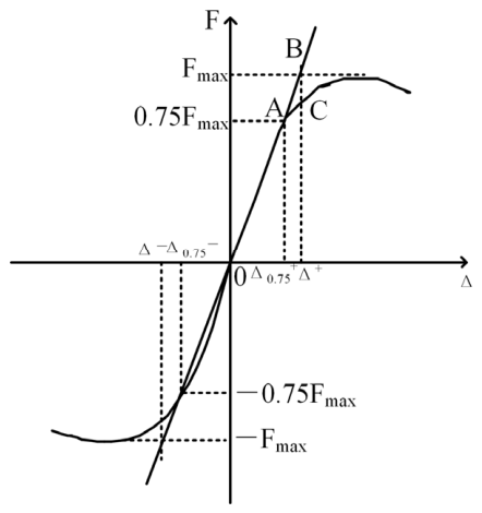
Several methods have been proposed for identifying the yield point. The Park method is widely adopted because it avoids the uncertainty associated with direct measurements of longitudinal-reinforcement strain [32,35]. As shown in Figure 4, the initial secant stiffness is determined using the point corresponding to 0.75 Fpk, and the equivalent yield displacement is obtained from the intersection of the extended secant line with the peak-strength level.

When a force–displacement backbone curve is unavailable, the yield parameters can be estimated using an equivalent plastic-hinge model. For a flexure-dominated cantilever pier, the yield displacement and yield strength may be calculated as [32,36]

$${\Delta }_{y=}{\displaystyle \frac{L_y^{2\varphi }}{3}}$$

(12)

$$F_{y=}{\displaystyle \frac{M_y}{L}}$$

(13)

where $L$ is the pier height, and $M_y$ and ${\varphi }_y$ are the sectional yield moment and yield curvature, respectively. These quantities can be obtained from moment–curvature analysis.

For circular and rectangular sections, the yield curvature may also be approximately estimated using the expressions recommended in JTG/T 2231-01-2020 [36]:

For circular sections:

$${\varphi }_{y}D=2.213{\epsilon }_y$$

(14)

For rectangular sections:

$${\varphi }_{y}H=1.957{\epsilon }_y$$

(15)

where D is the diameter of the circular section; H is the section depth in the loading direction; and εy is the yield strain of the longitudinal reinforcement.

The initial stiffness may alternatively be estimated as [37]

$$k_{e=}{\displaystyle \frac{{3\left(EI\right)}_{eff}}{L^3}}$$

(16)

where ${\left(EI\right)}_{eff}$ is the effective flexural stiffness determined using an applicable code or an experimentally validated relationship.

Accordingly, the yield force $F_y$ can also be calculated from the yield displacement ${\mathsf{\Delta }}_y$, obtained using the simplified formula and the elastic stiffness $k_e$ determined from the following empirical formula:

$$F_y=k_e{∆}_y$$

(17)

For the peak point, it can be directly obtained when the force–displacement backbone curve of the component is available. If the force–displacement backbone curve is unavailable, the peak force and its corresponding displacement can be determined through sectional analysis. Assuming that all plane sections perpendicular to the member axis remain planar after deformation, the strain distribution in the compression zone is linear. Thus, the concrete strain ${\epsilon }_c$ at a distance $x$ from the neutral axis satisfies ${\epsilon }_c=\varphi x$. Accordingly, the resultant compressive force of the concrete, $C_c$, within the compression-zone depth $c$ can be expressed as [32,38]

$$C_c={\displaystyle {\int }_0^c}b{\sigma }_{c}dx$$

(18)

where $b$ is the section width and ${\sigma }_c$ is the concrete stress. The general expression of the Hognestad model can flexibly and reasonably represent the fundamental compressive behavior of concrete. Therefore, the concrete constitutive relationship proposed by Hognestad is commonly adopted [32]:

$${\sigma }_c=\left\{\begin{array}{c}{f}_c\left[{2\epsilon }_c/{\epsilon }_{co}-{\left({2\epsilon }_c/{\epsilon }_{co}\right)}^2\right] {\epsilon }_c\le {\epsilon }_{co}\\ f_c-\left({\epsilon }_c-{\epsilon }_{co}\right)\left[0.15f_c/\left({\epsilon }_{c85}-{\epsilon }_{co}\right)\right] {\epsilon }_{co}{<\epsilon }_c\le {\epsilon }_{cu}\end{array}\right.$$

(19)

where ${\epsilon }_{co}$ is the concrete strain corresponding to the peak stress, generally taken as 0.002; ${\epsilon }_{c85}$ is the concrete strain when the stress decreases to $0.85f_c$; and ${\epsilon }_{cu}$ is the ultimate compressive strain of concrete.

A bilinear constitutive model is adopted for reinforcing steel under both tension and compression, with equal tensile and compressive strengths assumed. The tensile constitutive relationship is given by [32]

$${\sigma }_{st}=\left\{\begin{array}{c}{E}_s{\epsilon }_{st} {\epsilon }_{st}\le {\epsilon }_y\\ f_y+E_p\left({\epsilon }_{st}-{\epsilon }_y\right) {\epsilon }_y{<\epsilon }_{st}\le {\epsilon }_u\end{array}\right.$$

(20)

where ${\sigma }_{st}$ is the stress in the reinforcing steel; ${\epsilon }_{st}$ is the tensile strain of the reinforcing steel; ${\epsilon }_y$ is the yield strain of the reinforcing steel; ${\epsilon }_u$ is the ultimate strain of the reinforcing steel; $E_s$ is the elastic modulus of the reinforcing steel; and $E_p$ is the post-yield tangent modulus of the reinforcing steel.

According to the plane-section assumption, the resultant tensile force in the longitudinal reinforcement, $T_s$, is given by

$$T_s=\left\{\left[\varphi \left(h_o-c\right)-{\epsilon }_y\right]E_p+f_y\right\}{A}_s$$

(21)

where $h_o$ is the effective depth of the section and $A_s$ is the cross-sectional area of the longitudinal reinforcement in tension. Similarly, the resultant compressive force in the longitudinal reinforcement, $C_s$, is expressed as

$$C_s=\left\{\left[\varphi \left(h_o-a_s^{’}\right)-{\epsilon }_y\right]E_p+f_y\right\}{A}_s^{’}$$

(22)

where $A_s^{’}$ is the cross-sectional area of the longitudinal reinforcement in compression. By assuming that the resultant compressive force of the concrete acts at the midpoint of the compression zone and taking moments about the section centerline, the peak flexural moment of the section, $M_{pk}$, can be obtained as

$$M_{pk}=T_s\left(h_o-h/2\right)+C_s\left(h/2-a_s^{’}\right)+C_c\left(h/2-c/2\right)$$

(23)

Neglecting the influence of second-order gravity effects, the peak lateral resistance of the bridge pier, $F_{pk}$, is given by

$$F_{pk}=M_{pk}/L$$

(24)

According to the equivalent plastic-hinge model, the peak displacement ${\mathsf{\Delta }}_{pk}$ can be expressed as

$${\mathsf{\Delta }}_{pk}={\mathsf{\Delta }}_y+\left({\varphi }_{pk}-{\varphi }_y\right)L_p\left(L-L_p/2\right)$$

(25)

where ${\varphi }_{pk}$ is the curvature corresponding to the peak force and $L_p$ is the equivalent plastic-hinge length, which can be determined using empirical formulas.

For the post-peak deterioration stiffness, when the force–displacement backbone curve of the component is available, it can be calculated from the slope of the line connecting the peak point and the ultimate point. When the force–displacement backbone curve is unavailable, based on the experimental results reported by Wibowo et al., the post-peak deterioration stiffness $k_{deg}$ is mainly related to the axial compression ratio η and the shear-span ratio$\left(L/h\right)$, and can be calculated as [37]

$$k_{deg}=\left(0.3e^{5.7\eta }\right)/\left[\left(9-L/h\right){\mathsf{\Delta }}_y\right]$$

(26)

LeBorgne et al. suggested a residual-to-peak-strength ratio of F_r/F_pk = 0.2; thus, F_r = 0.2F_pk. In the residual-to-yield strength notation adopted in Equation (3), this recommendation corresponds to k_ry = 0.2k_py, rather than k_ry = 0.2. The ultimate displacement Δ_u is recommended as 1.2Δ_a, where Δ_a is the zero-strength intercept of the line descending from F_pk with slope k_deg. It is calculated using Equation (27) [32,39].

$${\mathsf{\Delta }}_a=F_{pk}/k_{deg}+{\mathsf{\Delta }}_{pk}$$

(27)

In summary, the backbone curve of the IMK model is characterized by seven parameters when symmetric hysteretic behavior is assumed: the elastic stiffness $k_e$; the displacement interval from yield to peak, ${\Delta }_p = {\Delta }_{pk} - {\Delta }_y$; the displacement interval from the peak to the zero-strength point, ${\Delta }_{pc} = {\Delta }_a - {\Delta }_{pk}$; the ultimate displacement ${\Delta }_u$; the yield force $F_y$; the peak-to-yield strength ratio $k_{py} = F_{pk}/F_y$; and the residual-to-yield strength ratio $k_{ry} = F_r/F_y$. Except for the elastic stiffness $k_e$, the remaining six parameters may take different values in the positive and negative loading directions.

2.3. Fiber-Based Finite Element Model

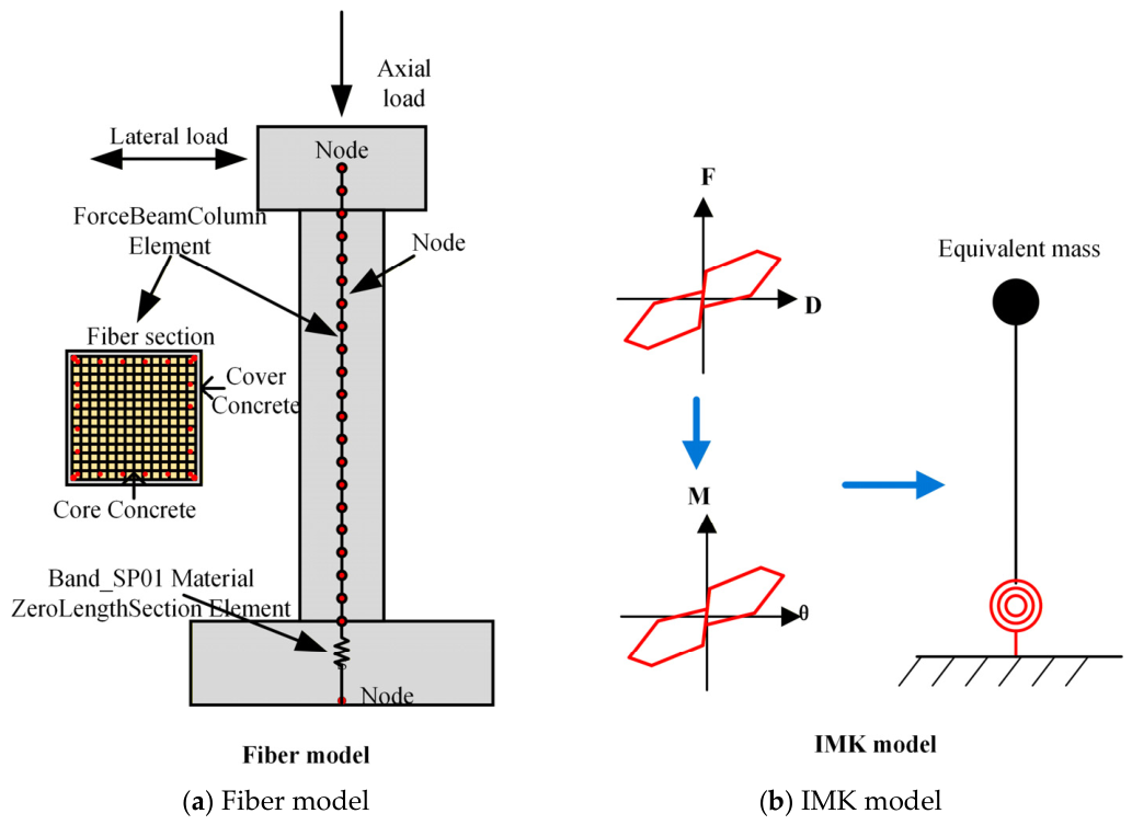
To provide a detailed numerical benchmark for evaluating the simplified IMK model, a fiber-based finite-element model was developed in OpenSees. As shown in Figure 5, the pier shaft was discretized using displacement-based nonlinear beam-column elements. Sectional response was evaluated at the integration points, geometric nonlinearity was represented using a P–Δ transformation, and each reinforced-concrete section was divided into confined core-concrete, unconfined cover-concrete, and longitudinal-reinforcement fibers [40,41].

The cyclic behavior of concrete was simulated using Concrete02, which follows the Kent–Scott–Park formulation. This material represents nonlinear compression, unloading stiffness degradation, and linear tension softening. The properties of the confined core concrete were determined using the Mander confinement model, considering the spacing, volumetric ratio, and yield strength of the transverse reinforcement. The cover concrete was treated as unconfined concrete [38].

The longitudinal reinforcement was simulated using the ReinforcingSteel material in OpenSees. The model represents yielding, strain hardening, cyclic unloading and reloading, and the Bauschinger effect, enabling the steel–concrete interaction to be evaluated at the fiber level [42].

Strain penetration of longitudinal bars at the pier base can produce additional slip and fixed-end rotation. To account for this effect, zero-length interface elements were introduced at the pier-footing connection. The anchorage-slip response was represented using the BarSlip material in OpenSees, with parameters obtained from the concrete strength, reinforcement properties, bar diameter, development length, and number of anchored bars. The relevant degrees of freedom were constrained to ensure compatibility between the pier shaft and foundation [43,44].

At the specimen level, the resulting model combines distributed flexural nonlinearity along the pier shaft with localized anchorage-slip and rotational responses at the pier base. It was subsequently used as the refined numerical benchmark for comparison with the simplified concentrated-plasticity IMK model [45,46].

3. Experimental Calibration and Calibration-Set Assessment

3.1. Test Specimens and Experimental Program

The experimental database adopted in this study was obtained from quasi-static cyclic tests of urban rail RC solid piers previously reported by Duan et al. [47]. Ref. [47] reported the specimen designs, material properties, damage observations, parametric cyclic trends, Fiber-model validation, full-scale multiparameter analyses, ductility-based limit-state capacities, and PGA-based fragility results. Here, the data are reprocessed for a direction-specific IMK backbone and deterioration-parameter identification, followed by paired accuracy–efficiency comparisons with the Fiber representation. These IMK-specific calibration and benchmarking tasks constitute the new specimen-to-system contribution of the present manuscript.

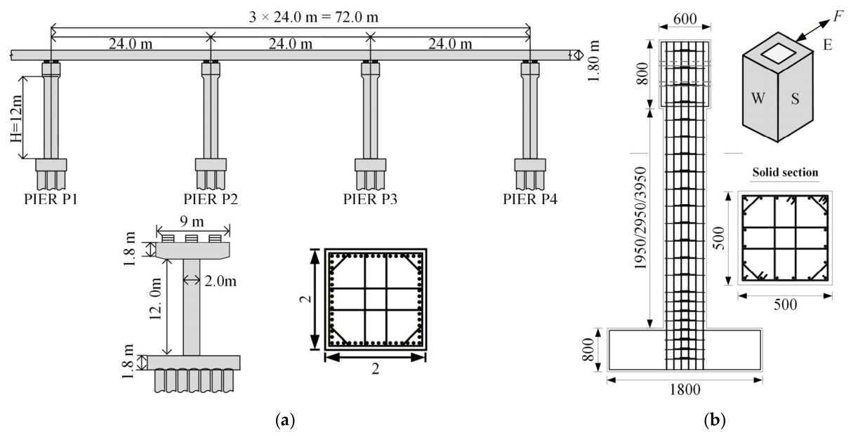
The test specimens were designed at a geometric scale of 1:4 based on a prototype urban rail viaduct bridge. The prototype arrangement and the selected pier are shown in Figure 6a, and the dimensions and reinforcement configuration of the scaled specimens are shown in Figure 6b. Each specimen consisted of a loading stub, a 500 mm × 500 mm square pier column, and an RC footing. The pier height varied from 1.95 to 3.95 m, while the footing and loading-stub details were kept constant to maintain consistent boundary conditions.

A total of seven specimens, designated A1–A3, B1–B2, and C1–C2, were divided into three groups according to the investigated parameter. Group A was designed to examine the effect of the aspect ratio by varying the pier height while maintaining the section and reinforcement details. Group B investigated the effect of transverse reinforcement by changing the stirrup spacing and volumetric transverse reinforcement ratio. Group C examined the effect of the longitudinal reinforcement ratio. The axial load ratio was maintained at 0.05 for all specimens. The principal design parameters are summarized in

Table 1. Design parameters and experimental program of the scaled RC solid-pier specimens.

Group	Specimen	$\mathbf{L}$ (m)	Longitudinal Rebar		Stirrup
			Layout	${\mathit{\rho }}_{\mathit{l}}$ (%)	$\mathbf{s}$ (mm)	${\mathsf{\rho }}_{\mathbf{s}}$ (%)
A	A1	1.95	20φ16 + 4φ22	2.12	110	2.35
	A2	2.95	20φ16 + 4φ22	2.12	110	2.35
	A3	3.95	20φ16 + 4φ22	2.12	110	2.35
B	B1	2.95	8φ16 + 12φ22	1.79	70	2.44
	B2	2.95	8φ16 + 12φ22	1.79	140	1.22
C	C1	2.95	20φ16	1.13	95	1.78
	C2	2.95	4φ16 + 20φ22	2.43	95	1.78

Note: ${\rho }_l$ is the longitudinal reinforcement ratio, and ${\rho }_s$ is the volumetric transverse reinforcement ratio.

.

All specimens were constructed using C40 concrete. HRB400 reinforcing bars with diameters of 16 and 22 mm were used as the longitudinal reinforcement, whereas 10 mm diameter HRB335 bars were used as the transverse hoops and cross-ties. The measured compressive strength, tensile strength, and elastic modulus of the concrete were 42.5 MPa, 3.49 MPa, and 31.3 GPa, respectively. The measured yield and ultimate strengths were 442 and 635 MPa for the longitudinal reinforcement and 400 and 530 MPa for the transverse reinforcement, respectively. The measured material properties are summarized in

Table 2. Measured mechanical properties of the concrete and reinforcing steel.

Material	Grade	Diameter (mm)	Compressive Strength (MPa)	Tensile Strength (MPa)	Elastic Modulus (GPa)	Yield Strength (MPa)	Ultimate Strength (MPa)
Concrete	C40	-	42.5	3.49	31.3	-	-
Longitudinal reinforcement	HRB400	16/22	-	-	200	442	635
Transverse reinforcement	HRB335	10	-	-	200	400	530

.

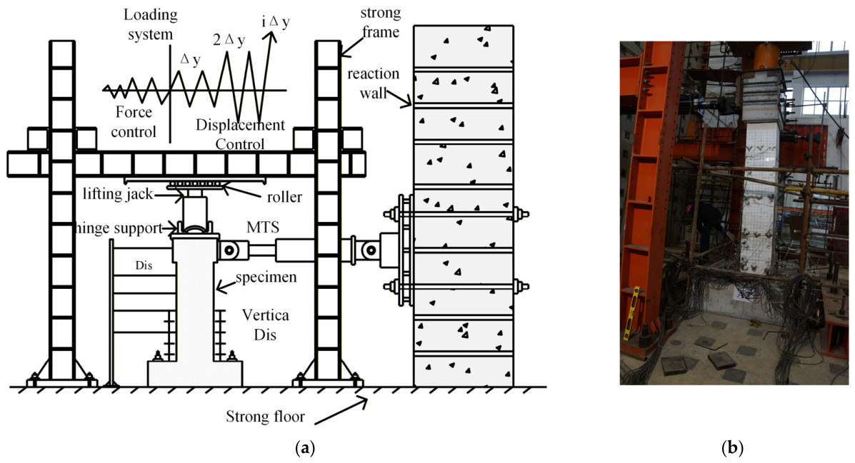
Quasi-static cyclic tests were conducted at the Road and Bridge Institute Laboratory of Sichuan Provincial Highway Planning, Survey, Design and Research Institute. As shown in Figure 7, the test system consisted of an axial loading device, a lateral loading device, and an instrumentation system. A constant axial load corresponding to an axial load ratio of 0.05 was applied using a hydraulic jack through a loading beam and a steel reaction frame. A sliding device beneath the jack allowed horizontal movement with the specimen, and reversed lateral loading was applied using a 1000-kN MTS servo-hydraulic actuator (Chengdu Huakongli Mechanical & Electrical Engineering Co., Ltd., Chengdu, China) with a stroke of ±300 mm.

A hybrid force–displacement loading protocol was adopted. Before yielding, the specimens were subjected to force-controlled loading with progressively increasing amplitudes, and two fully reversed cycles were imposed at each loading level. After yielding, the loading mode was changed to displacement control. The subsequent displacement amplitudes were defined as multiples of the measured yield displacement, ${\mathsf{\Delta }}_y$, with two fully reversed cycles applied at each displacement level. The tests were terminated when the lateral load-carrying capacity decreased to approximately 80% of the peak resistance.

Strain gauges were installed on selected longitudinal and transverse reinforcing bars to monitor the development of reinforcement strains. Linear variable differential transformers and surface displacement gauges were used to measure the global displacement, local deformation, and curvature response of the specimens. The lateral force and pier-top displacement histories recorded during the tests were subsequently used for IMK parameter identification and hysteretic-response comparison, as presented in Section 3.2.

3.2. Identification of Backbone Parameters and Calibration-Set Assessment

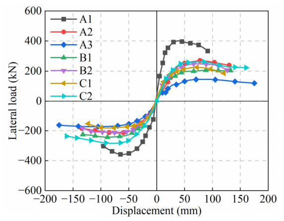
The experimental hysteretic responses of the seven specimens were processed to extract the corresponding backbone curves. For each loading direction, the force extrema attained during successive displacement cycles were selected and connected in ascending order of displacement amplitude. The positive and negative branches were processed independently to retain the directional asymmetry observed in the tests. The resulting backbone curves are presented in Figure 8.

The backbone curves of Group A exhibited a pronounced dependence on the aspect ratio. As the pier height increased from 1.95 m for A1 to 3.95 m for A3, the positive initial stiffness decreased from 21.416 to 3.228 kN/mm, while the peak resistance decreased from 396.10 to 144.40 kN. In contrast, the displacement corresponding to the positive peak resistance increased from 36.49 to 69.50 mm. Thus, the increase in aspect ratio reduced the lateral stiffness and strength but increased the absolute deformation developed before the peak response. For specimens B1 and B2, the differences in peak resistance were smaller than those observed in Group A, and the main differences occurred in the post-peak branches. This indicates that the transverse reinforcement primarily affected the stability of the response after the peak rather than producing a consistent increase in the initial stiffness. For Group C, increasing the longitudinal reinforcement ratio from 1.13% for C1 to 2.43% for C2 increased the positive yield force from 177.69 to 249.29 kN and the peak force from 226.06 to 263.04 kN. The corresponding normalized ultimate deformation also increased from 10.679 to 12.539.

The IMK backbone parameters were identified from the experimental backbone curves using the procedure described in Section 2.2. The equivalent yield point (Δ_y, F_y) was determined using the Park procedure, and the initial stiffness was calculated as

$$k_e={\displaystyle \frac{F_y}{{\Delta }_y}}$$

(28)

The experimental peak point was denoted by (Δ_pk, F_pk). A linear descending branch was subsequently established using the peak point and the force attained when the maximum displacement level was first reached. The intersection between this descending branch and the zero-force axis defined the zero-strength displacement, Δ₀. The normalized pre-peak, post-peak, and ultimate deformation parameters were then calculated as

$$U_{\mathrm{pre}}={\displaystyle \frac{{\Delta }_{pk}-{\Delta }_y}{{\Delta }_y}},$$

(29)

$$U_{\mathrm{post}}={\displaystyle \frac{{\Delta }_0-{\Delta }_{pk}}{{\Delta }_y}},$$

(30)

and

$$U_u={\displaystyle \frac{{\Delta }_0}{{\Delta }_y}}=1+U_{\mathrm{pre}}+U_{\mathrm{post}}.$$

(31)

The peak-to-yield strength ratio was defined as

$$k_{py}={\displaystyle \frac{F_{pk}}{F_y}}.$$

(32)

The identified positive- and negative-direction backbone parameters and specimen-specific cyclic parameters are summarized in

Table 3. Identified positive- and negative-direction IMK backbone parameters and specimen-specific cyclic parameters for the seven specimens.

Group	Specimen	Direction	Δy (mm)	Fy (kN)	ke (kN/mm)	Δpk (mm)	Fpk (kN)	Upre	Upost	Uu	kpy	${\mathit{c}}_{\mathit{K}}$	${\mathit{\kappa }}_{\mathbf{F}}$	${\mathit{\kappa }}_{\mathbf{D}}$
A	A1	+	15.06	322.52	21.41	36.49	396.10	1.42	12.24	14.67	1.23	0.45	0.72	0.60
		−	35.09	319.31	9.10	65.03	357.29	0.85	2.93	4.79	1.12
	A2	+	30.51	199.16	6.52	74.10	269.95	1.42	9.26	11.69	1.36	0.60	0.72	0.60
		−	35.09	319.31	9.10	65.03	357.29	0.85	2.93	4.79	1.12
	A3	+	34.41	111.05	3.22	69.50	144.40	1.02	12.27	14.29	1.30	0.60	0.72	0.60
		−	35.09	319.31	9.10	65.03	357.29	0.85	2.93	4.79	1.12
B	B1	+	44.02	200.23	4.54	76.24	220.92	0.73	6.95	8.68	1.10	0.90	0.90	0.75
		−	44.14	224.26	5.08	84.21	252.60	0.91	4.67	6.58	1.13
	B2	+	33.00	204.08	6.18	64.06	249.51	0.94	9.28	11.23	1.22	0.45	0.72	0.60
		−	41.79	191.75	4.59	75.56	210.73	0.81	9.10	10.91	1.10
C	C1	+	23.97	177.69	7.41	72.13	226.06	2.01	7.70	10.68	1.27	0.45	0.72	0.60
		−	27.94	153.61	5.50	73.94	179.92	1.65	7.31	9.96	1.17
	C2	+	41.10	249.29	6.06	75.23	263.04	0.83	10.71	12.54	1.06	0.65	0.72	0.60
		−	50.94	265.92	5.22	86.83	281.04	0.70	7.97	9.68	1.06

Note: Positive- and negative-direction backbone parameters are reported as absolute magnitudes. The cyclic parameters c_K, κ_F, and κ_D were shared by both loading directions for each specimen. Symbols “+” and “−” denote the positive loading direction and the reverse loading direction, respectively.

. The backbone parameters were identified independently for the two loading directions, whereas the cyclic parameters were shared by both directions for each specimen.

Following the identification of the positive- and negative-direction backbone parameters using the procedure described in Section 2.2, these parameters were held fixed during cyclic calibration. The initial cyclic-parameter values were selected from the ranges and parameter-response trends reported in previous IMK studies [31,32]. The cyclic parameters were then adjusted sequentially according to their dominant effects on the experimental response. The unloading-deterioration exponent c_K was first adjusted to reproduce unloading stiffness degradation, followed by κ_F and κ_D to reproduce pinching and reloading behavior. The energy-based deterioration parameters were calibrated to reproduce repeated-cycle strength loss and the hysteretic-loop area without automated optimization or a single scalar objective. Calibration ended when further adjustment produced no meaningful improvement. Throughout this process, κF and κD were restricted to physically meaningful ranges, and all deterioration parameters remained positive.

The common cyclic parameters not listed in Table 3 were calibrated against the complete experimental loops by iteratively matching unloading stiffness degradation, reloading pinching, repeated-cycle strength loss, and enclosed loop area. The specimen-specific values of cK, κF, and κD are summarized in Table 3. This iterative response-matching process is an engineering calibration rather than an independent prediction or demonstration of a unique global optimum. Analyst dependence and the absence of a specimen-level hold-out dataset remain limitations of the present workflow. A systematic quantitative sensitivity analysis of these cyclic parameters was not conducted.

Although no independent hold-out specimen was available, identification was mechanically constrained rather than based on unrestricted curve fitting. Backbone control points were fixed before cyclic calibration as described in Section 2.2. For the tested specimens, yield, peak strength, post-capping response, residual strength, and ultimate deformation were derived from measured directional backbones using fixed definitions. When test data are unavailable, Section 2.2 provides sectional-analysis and equivalent-plastic-hinge estimates. Only deterioration and pinching parameters were subsequently adjusted. For the full-scale model, the IMK backbone was extracted once from the first-cycle Fiber envelope and held fixed during dynamic and IDA analyses. These comparisons assess consistency across loading histories and intensities, not out-of-sample validity; applicability therefore remains limited to the calibration domain.

The identified force–displacement parameters were transformed into the moment-rotation parameters required by the concentrated-plasticity model using work-consistent cantilever relations. For a specimen of height L, lateral force and pier-top displacement were converted as M = FL and θ = Δ/L; consequently, the rotational spring stiffness was K_θ = k_eL². The same conversion was applied to the positive and negative yield, peak, post-capping, residual, and ultimate points. An elastic pier element represented the response outside the plastic-hinge region, and a zero-length IMK rotational spring was assigned at the pier base. Positive and negative backbone parameters were retained separately to reproduce the measured directional asymmetry.

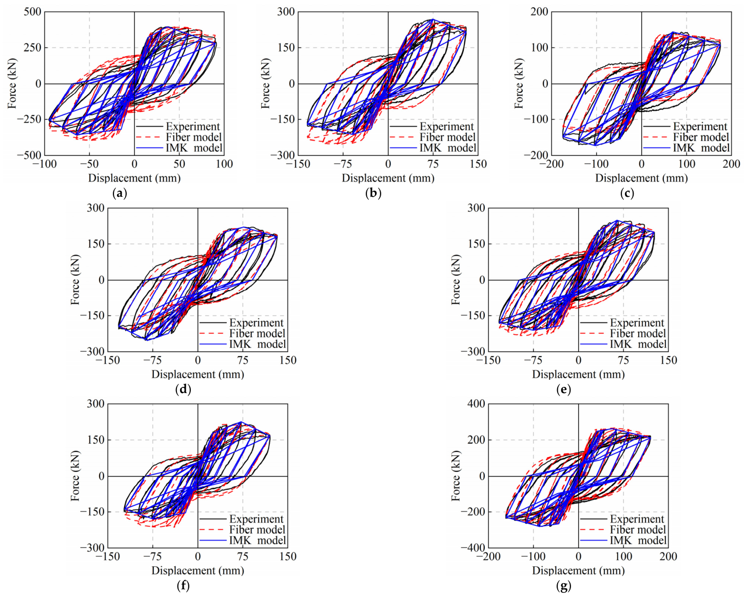
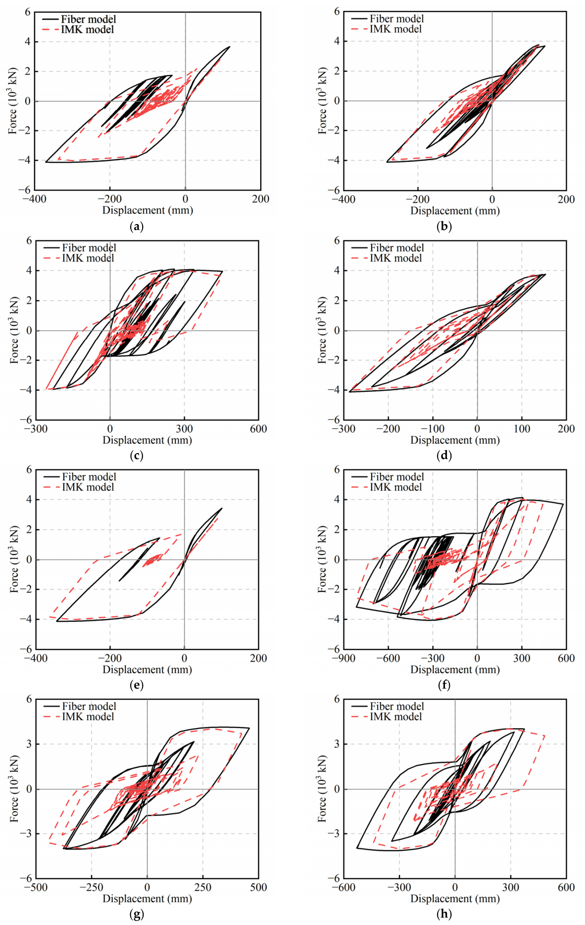
For comparison, the previously developed Fiber models were retained as refined numerical references. Both models were subjected to the same displacement histories as the corresponding tests. The experimental, Fiber-model, and IMK-model hysteretic responses are compared in Figure 9.

As shown in Figure 9, both numerical approaches reproduced the overall evolution from the approximately linear initial response to the nonlinear post-yield response. The Fiber models generally captured the overall hysteretic shape and produced relatively full loops, although deviations occurred in the peak-force locations and directional asymmetry for several specimens.

Because the IMK backbone parameters were identified directly from the experimental curves, the simulated yield and peak points were expected to coincide closely with the corresponding test values in both loading directions. The agreement at those control points demonstrates faithful transfer of the calibration targets, not independent predictive validation. The models also retained the principal specimen-to-specimen changes in initial stiffness, peak resistance, post-peak degradation, and directional asymmetry.

Differences between the IMK and experimental responses were mainly observed in the unloading and reloading branches. The IMK hysteretic loops were generally narrower than the experimental loops, particularly for specimens A3, B1, and C2, indicating that the simplified model underestimated part of the cyclic energy dissipation. In contrast, the Fiber models generally produced fuller loops, although their peak forces and the displacement coordinates of the peaks were less consistent with the experimental values in several cases. Therefore, the IMK model provided a more direct reproduction of the experimentally identified backbone response, whereas the Fiber model retained greater detail in the distributed nonlinear and cyclic response.

Overall, the calibration-set comparisons show that the simplified IMK model captures the global hysteretic characteristics considered in the subsequent analyses, including initial stiffness, lateral strength, deformation capacity, strength degradation, and positive–negative asymmetry. The remaining discrepancies in energy dissipation, unloading stiffness, and loop shape are quantified in Section 3.3. Predictive capability outside the seven calibration specimens is not established by this comparison and requires hold-out specimens or an independent database.

3.3. Quantitative Evaluation of Calibration-Set Accuracy

Because the yield, peak, and post-peak control points were used to identify the IMK backbone and the complete loops informed the cyclic-parameter matching, the same-specimen comparisons do not constitute independent validation; they quantify calibration-set accuracy. To reduce direct dependence on the backbone control points, performance was additionally evaluated using the evolution of cumulative normalized hysteretic energy and the specimen-level residual displacement, total cumulative hysteretic energy, and secant stiffness. These quantities emphasize unloading and reloading paths, pinching, cyclic deterioration, and enclosed loop area, but they remain derived from the calibration specimens and therefore do not demonstrate out-of-sample prediction.

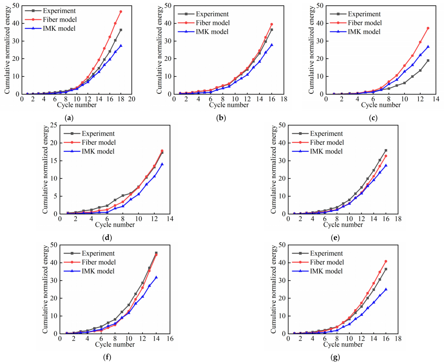
The hysteretic energy dissipated during each complete loading cycle was calculated from the area enclosed by the force–displacement loop. Displacement and force were normalized by the experimental yield values, and the normalized energy was accumulated sequentially. As shown in Figure 10, the cumulative normalized hysteretic energy increases slowly during the initial elastic and mildly inelastic loading stages and rises rapidly after the specimens undergo large-amplitude cyclic deformation. Both numerical models generally reproduce the experimentally observed evolution of cumulative energy dissipation. The Fiber model tends to predict greater cumulative energy dissipation for most specimens, whereas the IMK model generally produces lower cumulative values than the experimental results. This difference becomes more pronounced during the later large-amplitude cycles because the accumulated energy is sensitive to differences in the predicted loop area, pinching behavior, and cyclic deterioration. Specimen A3 exhibits a comparatively large overestimation by both numerical models, indicating greater sensitivity of its hysteretic-energy response to the adopted constitutive and deterioration assumptions. Nevertheless, the two models capture the principal accumulation trend in the normalized hysteretic energy for the seven specimens.

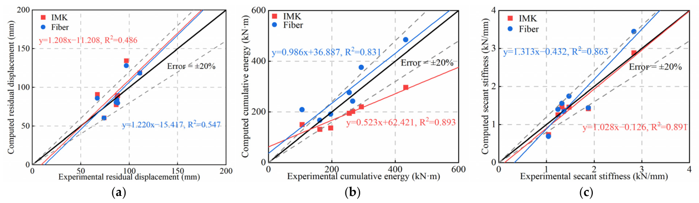
To quantify specimen-level agreement, diagonal-error comparisons were performed for residual displacement, final cumulative hysteretic energy, and secant stiffness, as shown in Figure 11. The experimental result is plotted on the horizontal axis, the numerical result on the vertical axis, and the 1:1 line denotes perfect agreement.

The residual displacement was defined as the absolute displacement at the final zero-force crossing of the last common complete hysteretic loop. As shown in Figure 11a, both models reproduce the general magnitude of the experimentally measured residual displacement, with mean absolute percentage errors of 15.06% and 15.98% for the Fiber and IMK models, respectively. However, the corresponding coefficients of determination are only 0.547 and 0.486. The relatively large scatter indicates that residual displacement is more difficult to reproduce consistently than the other response indices. This quantity is particularly sensitive to small differences in the unloading path, force-zero crossing, displacement offset, and asymmetric pinching behavior. Consequently, the residual-displacement results should be interpreted as an assessment of the overall magnitude rather than a highly stable specimen-to-specimen correlation. In addition to the three response indices presented in Figure 11, the prediction errors of the Fiber model in terms of peak lateral strength and ultimate deformation capacity were quantified for all seven specimens. The corresponding mean absolute percentage errors were 6.1% and 9.6%, respectively. Taken together, these results provide a quantitative basis for evaluating the accuracy and limitations of the Fiber model as the refined numerical benchmark.

Figure 11b compares the cumulative hysteretic energy obtained by summing the enclosed areas of all common complete loading cycles. The Fiber and IMK models achieve coefficients of determination of 0.831 and 0.893, respectively, demonstrating that both models reproduce the relative variation in energy-dissipation capacity among the seven specimens. The Fiber-model regression slope is close to unity, although its mean absolute percentage error is 22.76%. The IMK model exhibits a higher coefficient of determination but a mean absolute percentage error of 27.79%. Moreover, its regression slope is substantially lower than unity, indicating an increasing tendency to underestimate cumulative energy as the experimental energy demand increases. This result is consistent with the smaller loop areas observed in the cycle-by-cycle normalized-energy comparisons.

The secant stiffness was evaluated from the chord connecting the positive and negative peak points of the final common complete cycle. As shown in Figure 11c, the Fiber and IMK models yield coefficients of determination of 0.863 and 0.891, respectively. The corresponding mean absolute percentage errors are 18.52% and 9.93%. Among the three diagonal-error indices, the IMK model provides the closest quantitative agreement for the secant stiffness, with a regression slope close to unity and a relatively small intercept. This demonstrates that the simplified model reliably reproduces the global stiffness level of the specimens under high cyclic deformation demands.

Overall, both numerical models reproduce the principal strength-independent characteristics of the calibration specimens. The Fiber model provides a relatively balanced representation of cumulative energy dissipation, whereas the IMK model achieves better agreement in final secant stiffness but tends to underestimate cumulative hysteretic energy. Residual displacement shows greater specimen-to-specimen scatter for both models because it is sensitive to unloading and pinching details. These calibration-set results support the use of the IMK model for global stiffness degradation and overall energy trends within the investigated domain, while its limitations in residual deformation, large-cycle energy dissipation, and out-of-sample prediction must be retained in subsequent interpretations.

4. Dynamic Response Analysis of the Full-Scale Bridge Pier

4.1. Prototype Pier

A full-scale analytical prototype model was established based on the prototype urban-rail viaduct from which the quarter-scale pier specimens described in Section 3.1 were derived. The geometric dimensions, sectional properties, material parameters, mass distribution, and boundary conditions of the prototype bridge were adopted in the full-scale model. A three-dimensional finite-element model was first developed in SAP2000, and modal analysis was conducted to determine the global dynamic characteristics of the bridge. Subsequently, the Fiber and IMK models were established in OpenSees using consistent structural configurations and dynamic parameters. The SAP2000 model was employed as the reference model for evaluating the initial dynamic characteristics of the two OpenSees models.

The prototype deck, pier, and support arrangement is shown in Figure 6a, while the adopted mass distribution and boundary conditions follow the prototype configuration. In the Fiber model, each 12 m pier shaft was discretized into 22 displacement-based nonlinear beam-column elements with three integration points per element. Confined concrete, cover concrete, and longitudinal reinforcement were represented by the sectional fibers described in Section 2.3. The damping and P-Delta treatments are detailed in Section 4.3 and Section 4.2, respectively.

The first three natural periods obtained from the three numerical models are summarized in

Table 4. Natural periods, cumulative longitudinal mass-participation ratios, and dominant mode shapes obtained from the IMK, Fiber, and SAP2000 models.

Mode	IMK (T) (s)	Fiber (T) (s)	SAP2000 (T) (s)	Mean Period (s)	Frequency (Hz)	Cumulative Longitudinal Mass-Participation Ratio, X (%)	Dominant Mode Shape
1	1.274	1.323	1.291	1.296	0.772	79.27	Longitudinal translation of the bridge deck and piers
2	0.817	0.879	0.842	0.846	1.182	79.27	Global transverse bending
3	0.536	0.594	0.574	0.568	1.761	79.27	Deck torsion coupled with higher-order bending

. For the first mode, the natural periods predicted by the IMK, Fiber, and SAP2000 models were 1.274, 1.323, and 1.291 s, respectively. The mean fundamental period was 1.296 s, corresponding to a frequency of 0.772 Hz. Therefore, T1 = 1.296 s was adopted as the representative fundamental period for the subsequent ground-motion classification and seismic-response analyses.

For the second mode, the natural periods predicted by the three models were 0.817, 0.879, and 0.842 s, respectively, with a mean period of 0.846 s and a corresponding frequency of 1.182 Hz. This mode was characterized by the global transverse bending of the bridge. The third-mode periods obtained from the IMK, Fiber, and SAP2000 models were 0.536, 0.594, and 0.574 s, respectively. The resulting mean period and frequency were 0.568 s and 1.761 Hz, respectively. The third mode primarily involved deck torsion coupled with higher-order bending deformation of the piers. Modes 2 and 3 contributed negligibly to the longitudinal response, so the cumulative X-direction mass-participation ratio remained 79.27% throughout the third mode. It reached 91.32% when the first 11 modes were included.

Taking the SAP2000 periods as a reference, the relative differences in the first three periods predicted by the IMK model were 1.32%, 2.97%, and 6.62%, respectively, while those of the Fiber model were 2.48%, 4.39%, and 3.48%. The maximum difference was 6.62%. The three models therefore exhibited consistent periods, providing a common basis for the subsequent comparison of nonlinear response, computational efficiency, and fragility.

4.2. Quasi-Static Benchmarking and Identification of Full-Scale IMK Parameters

Following the comparison of the dynamic characteristics presented in Section 4.1, reverse-cyclic analyses were conducted to identify the IMK parameters of the full-scale analytical pier and compare its quasi-static response. The Fiber model was generated from specimen A2 using a geometric scale factor of four while preserving material properties, reinforcement ratios, equivalent steel areas, and axial-load ratio. Its first-cycle force–displacement response was then used to identify the equivalent IMK backbone. Accordingly, the Fiber model is a calibration benchmark for the simplified representation at this level, not independent full-scale validation evidence.

The 12 m pier was obtained by geometric scaling while maintaining the material properties, reinforcement ratios, and axial-load ratio of specimen A2. Preserving these principal design ratios provides a reasonable basis for comparing the global flexural responses of the Fiber and IMK models. Nevertheless, possible size effects on bond slip, crack localization, confinement, and cyclic deterioration are not explicitly reproduced. Therefore, transferring the specimen-calibrated hysteretic assumptions to the 12 m pier should be regarded as an analytical modeling assumption.

The IMK backbone parameters were extracted from the first-cycle envelope of the Fiber response using the procedure described in Section 2.2. The positive and negative yield points were (120 mm, 3685.46 kN) and (−120 mm, −3704.72 kN), and the corresponding peak points were (300 mm, 4040.49 kN) and (−300 mm, −4024.58 kN). Linear extrapolation of the post-peak branches gave zero-strength displacement intercepts of 1845.59 and 1723.79 mm. The resulting parameters are summarized in

Table 5. Equivalent global IMK parameters identified for the full-scale pier.

Direction	Δy (mm)	ke (kN/mm)	Fy (kN)	Upre	Upost	Uu	kpy
Positive	120	30.712	3685.46	1.500	12.880	15.380	1.096
Negative	120	30.873	3704.72	1.500	11.865	14.365	1.086

.

The full-scale IMK model retained the cyclic parameters calibrated for specimen A2: ΛS = ΛC = 500; ΛA = 271; ΛK = 72; cS = cC = cA = 1.0; cK = 0.60; D+ = D− = 1.0; κF = 0.72; and κD = 0.60.

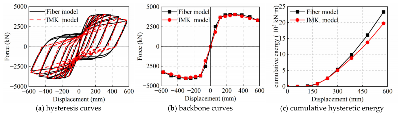
In the Fiber model, P–Δ effects were explicitly included through the OpenSees PDelta transformation under a constant 12.8 MN axial load. The extracted first-cycle backbone therefore incorporated the resulting reduction in lateral restoring force. The equivalent IMK model used a linear transformation without an additional geometric stiffness contribution, so P–Δ was represented once through the calibrated envelope and was neither omitted nor double-counted. This fixed envelope was retained in the dynamic and IDA analyses. However, it cannot update P–Δ effects under variable axial force, bidirectional interaction, or responses outside the calibration domain, for which explicit geometric nonlinearity is required. Figure 12 compares the quasi-static responses.

As shown in Figure 12a, both models reproduce the principal response stages of the full-scale pier, including the transition from the pre-yield response to strain hardening, the attainment of the peak lateral strength, and the subsequent post-peak strength degradation. The maximum lateral strengths of both models occur at a pier-top displacement of approximately 300 mm. The overall hysteresis-loop shapes and force-development trends predicted by the IMK model are consistent with those obtained from the Fiber model, indicating that the simplified concentrated-plasticity model adequately represents the global nonlinear response of the full-scale pier.

The first-cycle backbone curves are compared in Figure 12b. For displacement levels from 120 to 576 mm, the mean absolute percentage difference between the bidirectional mean peak forces predicted by the two models is 2.24%. The yield, peak, and terminal points were used directly in identification; therefore, the 180, 240, 384, and 480 mm points assess interpolation between calibration controls, not independent full-scale prediction. At these four intermediate levels, the mean absolute percentage difference is 3.83%. At 300 mm, the bidirectional mean peak forces predicted by the Fiber and IMK models are 4032.53 and 4032.12 kN, respectively, a difference of 0.01%. These values quantify internal consistency with the Fiber calibration benchmark.

A relatively large difference occurs at the 60 mm loading level. The bidirectional mean peak forces obtained from the Fiber and IMK models are 2526.74 and 1842.70 kN, respectively, and the IMK model underestimates the Fiber-model result by 27.07%. This difference is mainly associated with the representation of the pre-yield response using a single equivalent secant stiffness. Such an idealization cannot simultaneously reproduce the relatively high initial tangent stiffness and the gradual pre-yield stiffness variation predicted by the distributed-plasticity Fiber model. Nevertheless, this discrepancy occurs within the nominally elastic response range and contributes only slightly to the total hysteretic energy.

Differences are also observed in the repeated-cycle response at large displacement amplitudes. At 576 mm, the ratio of the second-cycle to first-cycle mean peak force is 92.19% for the Fiber model, whereas it remains approximately 100% for the IMK model. Therefore, although the IMK model closely reproduces the overall strength envelope, it underestimates the within-amplitude cyclic strength deterioration predicted by the Fiber model.

The cumulative hysteretic-energy responses of the two models are compared in Figure 12c. The horizontal coordinate represents the imposed displacement amplitude, and each point denotes the cumulative energy after completion of the two loading cycles at the corresponding displacement level. As shown in Figure 12c, the cumulative hysteretic energy predicted by both models increases continuously with the displacement amplitude. Before yielding, the energy dissipated by the Fiber model is limited, whereas the IMK model exhibits almost no hysteretic energy because its response remains essentially linear elastic and its hysteresis loops have negligible enclosed areas.

After the displacement amplitude reaches 180 mm, the cumulative energies predicted by both models increase rapidly. At displacement amplitudes of 180 and 240 mm, the Fiber model gives cumulative energies of 895.13 and 2559.47 kN·m, respectively, while the corresponding IMK-model results are 863.53 and 2524.63 kN·m. The associated differences are only 3.53% and 1.36%, indicating close agreement during the initial inelastic response.

With increasing displacement amplitude, the difference between the two curves gradually increases. At 300, 384, and 480 mm, the IMK model underestimates the Fiber model’s cumulative energy by 6.08%, 10.26%, and 14.35%, respectively. At the maximum displacement amplitude of 576 mm, the cumulative hysteretic energies obtained from the Fiber and IMK models are 23,328.92 and 19,738.63 kN·m, respectively. Therefore, the IMK model reproduces 84.61% of the cumulative energy predicted by the Fiber model, corresponding to an underestimation of 15.39%.

The increasing energy difference at large displacement amplitudes is associated with the smaller enclosed areas of the IMK model’s loops and its limited reproduction of the repeated-cycle strength deterioration predicted by the Fiber model. The two models nevertheless show consistent cumulative-energy trends within this controlled comparison. Because the IMK backbone was identified from the same Fiber benchmark, the agreement supports subsequent comparative analyses but should not be interpreted as independent full-scale validation. Independent full-scale experimental evidence or a separately developed analytical benchmark would be required for that purpose.

4.3. Dynamic Response and Computational Efficiency

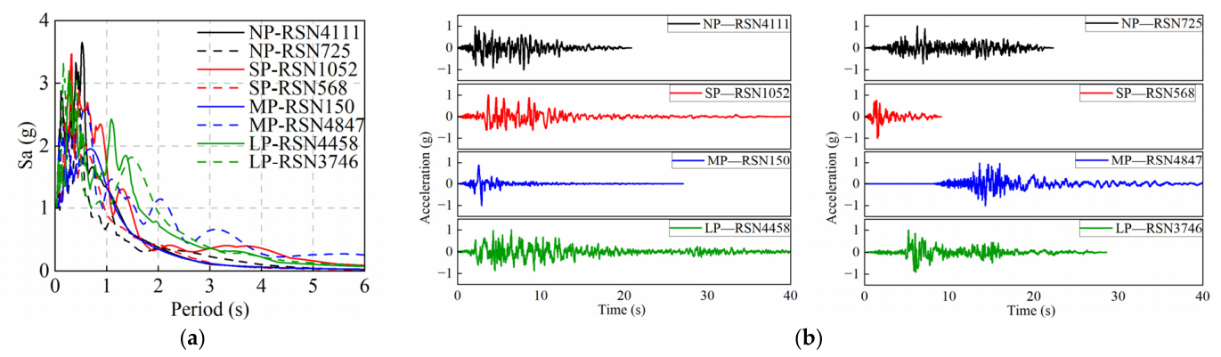
Eight representative ground motions were selected to compare the nonlinear dynamic responses predicted by the Fiber and IMK models. The set comprised two motions from each of the NP, SP, MP, and LP groups. Their principal characteristics are summarized in

Table 6. Basic information and pulse-period characteristics of the eight selected ground motions.

Type	RSN	Earthquake Event	${\mathit{M}}_{\mathit{w}}$	${\mathit{R}}_{\left(\mathit{r}\mathit{u}\mathit{p}\right)}$ (km)	${\mathit{V}}_{\left(\mathit{s}30\right)}$ (m/s)	${\mathit{T}}_{\mathit{p}}$ (s)	${\mathit{R}}_{\mathit{T}} = {\mathit{T}}_{\mathit{p}}/{\mathit{T}}_1$	Original PGA (g)	Scale Factor	$\mathbf{\Delta }\mathit{t}$ (s)
NP	4111	Parkfield-02, CA	6.00	2.67	297.46	—	—	0.2320	4.311	0.005
	725	Superstition Hills-02	6.54	11.16	316.64	—	—	0.4750	2.105	0.010
SP	1052	Northridge-01	6.69	7.26	508.08	0.728	0.562	0.3013	3.319	0.020
	568	San Salvador	5.80	6.30	489.34	0.805	0.621	0.7042	1.420	0.005
MP	150	Coyote Lake	5.74	3.11	663.31	1.232	0.951	0.4218	2.371	0.005
	4847	Chuetsu-oki	6.80	11.94	383.43	1.400	1.080	0.3031	3.299	0.010
LP	4458	Montenegro, Yugo.	7.10	5.76	318.74	1.974	1.523	0.2927	3.416	0.010
	3746	Cape Mendocino	7.01	18.31	459.04	1.967	1.518	0.3181	3.144	0.005

Note: NP, SP, MP, and LP denote non-pulse, short-period pulse-like, medium-period pulse-like, and long-period pulse-like ground motions, respectively. $M_w$ is the moment magnitude; $R_{\left(rup\right)}$ is the closest distance to the fault rupture plane; $V_{\left(s30\right)}$ is the time-averaged shear-wave velocity in the upper 30 m of soil; $T_p$ is the velocity-pulse period; $R_T=T_p/T_1$ is the relative pulse period, where the fundamental period of the bridge is $T_1=1.296 \mathrm{s}$; PGA is the peak ground acceleration; and $\Delta t$ is the time step of the record.

.

The selected records were scaled to PGA = 1.0 g before being applied to the two numerical models. The corresponding 5% damped acceleration response spectra and acceleration time histories are presented in Figure 13. A 5% damping ratio was assigned through mass-proportional Rayleigh damping calibrated at the fundamental period T₁ = 1.296 s; no stiffness-proportional damping term was used. For this formulation, $\alpha M = 2\xi 1\omega 1$ and ξ_n = ${\displaystyle \frac{\alpha M}{2\omega n}}= \xi 1\left({\displaystyle \frac{\omega 1}{\omega n}}\right)$. Accordingly, the implied damping ratios of the first three reported modes were 5.00%, 3.26%, and 2.19%, respectively, rather than a uniform 5%. The mass-only formulation avoids stiffness-proportional forces evaluated from a changing tangent stiffness and was applied identically to the Fiber and IMK models.

To examine the sensitivity to the damping implementation at the calibrated mode, supplementary response-history analyses were conducted for the eight representative ground motions at PGA = 1.0 g using a one-mode-compatible 5% modal-damping formulation, while all other modeling and analysis settings were kept unchanged. Relative to the baseline mass-proportional formulation, the mean absolute differences in peak pier-top displacement were 5.13 × 10⁻⁷% and 5.01 × 10⁻¹⁰% for the Fiber and IMK models, respectively, and the corresponding maximum differences were 1.92 × 10⁻⁶% and 1.84 × 10⁻⁹%. For peak base shear, the mean absolute differences were 2.12 × 10⁻¹¹% and 3.59 × 10⁻⁹%, with maximum differences of 1.04 × 10⁻¹⁰% and 7.19 × 10⁻⁹%, respectively. No systematic model- or ground-motion-group-dependent change was observed. The differences are at the level of numerical round-off, indicating that the principal Fiber–IMK response comparison is insensitive to these two one-mode-compatible damping implementations for the selected records and response quantities. This targeted check does not establish equivalence for alternative multi-mode damping targets or systems with stronger higher-mode participation.

To ensure a consistent comparison, the Fiber and IMK models were subjected to identical ground-motion inputs, gravity loads, damping assumptions, analysis durations, and numerical settings. The same local OpenSees executable was used for both models, while MATLAB R2024a was employed to manage the batch analyses and process the numerical results. All simulations were conducted serially using one worker on the same 64-bit Windows computer equipped with an Intel Core Ultra 7 265K processor operating at 3.90 GHz and 32.0 GB of RAM. The external wall-clock time was recorded for each analysis to evaluate computational efficiency.

Figure 14 compares the base-shear versus pier-top-displacement hysteretic responses. The IMK model reproduced the global envelope and peak resistance of the Fiber model. The relative differences in peak base shear for the eight records ranged from 1.62% to 3.56%, with a mean of 2.64%.

For RSN568, the peak base shears predicted by the Fiber and IMK models were 4122.9 and 3996.2 kN, respectively, corresponding to a relative difference of 3.07%. The hysteretic energies obtained by integrating the force–displacement responses were approximately $1.523\times {10}^3$ and $1.294\times {10}^3 \mathrm{k}\mathrm{N}·\mathrm{m}$, respectively. Thus, the IMK model underestimated the hysteretic energy under RSN568 by approximately 15.0%. This result indicates that the simplified model reproduced the peak resistance more accurately than the detailed area enclosed by the hysteretic loops.

For the records producing substantial inelastic deformation, the IMK model captured the principal force plateau and overall deformation range. This agreement was particularly evident for MP-RSN4847 and the two LP records. Differences remained in the unloading and reloading branches and in the areas enclosed by the internal hysteretic loops. The Fiber model explicitly represented the distributed cyclic responses of the concrete and reinforcement fibers along the pier. By contrast, the IMK model condensed these effects into a calibrated rotational spring at the pier base. Consequently, the simplified model reproduced the global response envelope more accurately than the detailed evolution of individual hysteretic cycles.

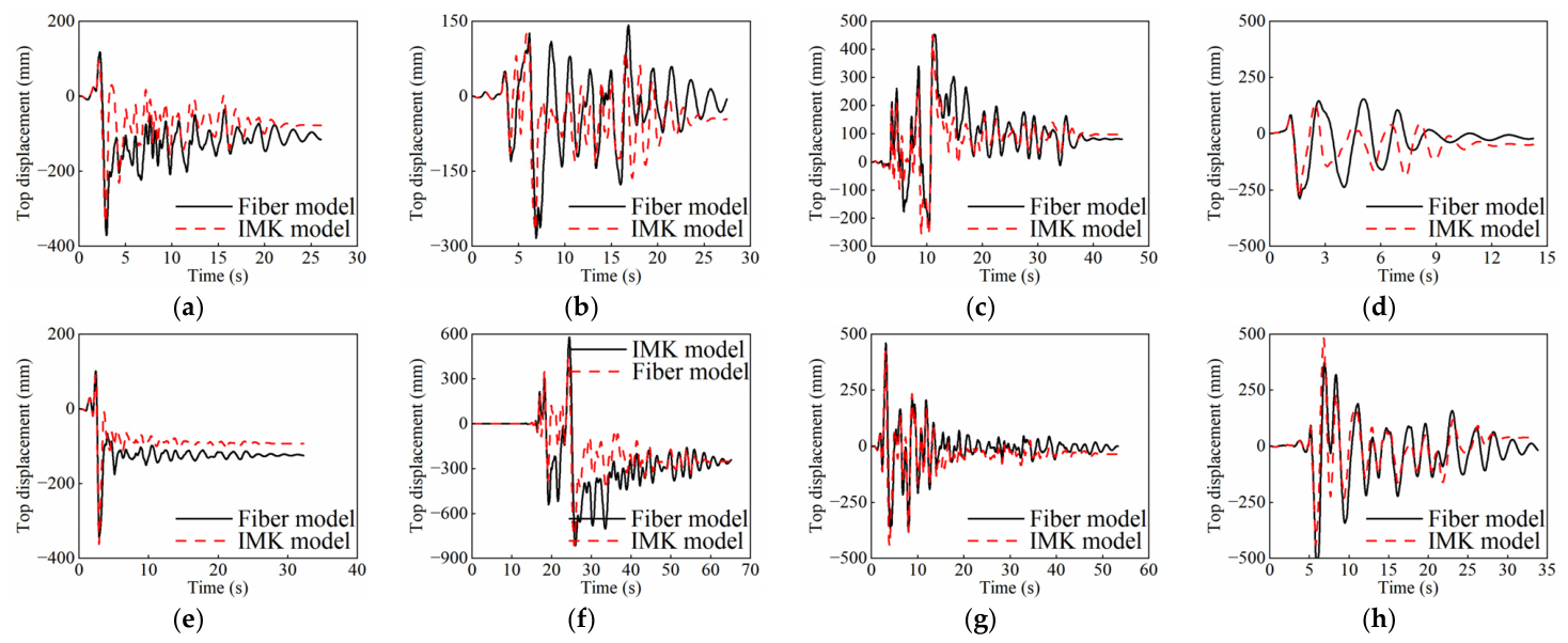
The corresponding pier-top displacement histories are presented in Figure 15. The maximum absolute pier-top displacement was defined as

$$D_{\mathrm{m}\mathrm{a}\mathrm{x}}={\mathrm{m}\mathrm{a}\mathrm{x}}_t\left|D\left(t\right)\right|$$

(33)

The relative error in the peak displacement predicted by the IMK model was calculated as

$$e_D=\left(\left|D_{\left(max,IMK\right)}-D_{\left(max,Fiber\right)}\right|\right)/\left(D_{\left(max,Fiber\right)}\right)\times 100\%$$

(34)

As summarized in

Table 7. Comparison of the maximum pier-top displacements and computational costs predicted by the Fiber and IMK models under the eight selected ground motions.

Type	Ground Motion	Fiber ${\mathit{D}}_{\mathbf{m}\mathbf{a}\mathbf{x}}$ (mm)	IMK ${\mathit{D}}_{\mathbf{m}\mathbf{a}\mathbf{x}}$ (mm)	Displacement Error (%)	Fiber Time (s)	IMK Time (s)	Speed-Up
NP	RSN4111	370.5	336.9	9.07	18.727	1.057	17.72
NP	RSN725	284.1	269.0	5.31	10.013	1.208	8.29
SP	RSN1052	453.9	450.9	0.66	19.963	0.906	22.04
SP	RSN568	287.8	284.1	1.29	9.913	0.845	11.73
MP	RSN150	344.5	362.5	5.23	18.836	1.134	16.61
MP	RSN4847	814.7	814.4	0.03	29.020	0.849	34.19
LP	RSN4458	458.8	446.6	2.65	26.720	0.741	36.08
LP	RSN3746	530.0	482.3	8.99	31.164	0.845	36.87

, the peak-displacement errors ranged from 0.03% to 9.07%, with a mean value of 4.15%. The mean errors for the NP, SP, MP, and LP records were 7.19%, 0.97%, 2.63%, and 5.82%, respectively. The IMK model predicted lower peak displacements for seven of the eight records, resulting in an overall signed bias of −2.85%. MP-RSN150 was the only record for which the IMK model predicted a higher peak displacement than the Fiber model, with an overestimation of 5.23%.

Among the selected ground motions, MP-RSN4847 generated the greatest displacement demand. The Fiber and IMK models predicted maximum pier-top displacements of 814.7 and 814.4 mm, respectively, with a relative error of 0.03%. This large response coincided with a pulse period close to the fundamental bridge period, but it cannot be attributed to period proximity alone because the selected records also differ in spectral amplitude, velocity content, duration, and other characteristics. The record dependence is evident from the two SP motions, which produced Fiber-model peak displacements of 453.9 and 287.8 mm despite sharing the same pulse-period category.

For RSN568, the maximum pier-top displacements predicted by the Fiber and IMK models were 287.8 and 284.1 mm, respectively, corresponding to a relative error of 1.29%. However, the residual displacements predicted by the two models were −22.47 and −49.77 mm, respectively. Therefore, close agreement in peak displacement did not necessarily indicate identical response phases, oscillation amplitudes, or residual deformations.

Agreement between the complete displacement histories was more variable than agreement between their peak values. The active-response correlation coefficients ranged from 0.346 to 0.918, with a mean value of 0.730. The normalized root-mean-square errors ranged from 9.52% to 32.58%, while the differences between the occurrence times of the peak responses ranged from 0.05 to 0.80 s. RSN568 had a peak-displacement error of only 1.29%, but its displacement-history correlation coefficient was 0.346. This comparison further demonstrates that accurate prediction of the maximum seismic demand does not necessarily imply that the complete nonlinear response history is reproduced with the same level of accuracy.

The computational efficiency of the two models was evaluated using external wall-clock time. The speed-up factor was calculated as the ratio of the Fiber-model time to the corresponding IMK-model time, using the definition given in Equation (48).

As shown in Table 7, the Fiber analyses required between 9.913 and 31.164 s per record, whereas the IMK analyses required only 0.741–1.208 s. The accumulated wall-clock times for the eight records were 164.356 s for the Fiber model and 7.584 s for the IMK model. The resulting overall speed-up factor was 21.67, corresponding to a 95.39% reduction in computational time. The group-level speed-up factors were 12.69, 17.07, 24.14, and 36.50 for the NP, SP, MP, and LP records, respectively. The larger speed-up factors obtained for the MP and LP records were mainly associated with the increased runtimes of the Fiber model, whereas the runtimes of the IMK model remained close to 1 s.

Overall, the IMK model reproduced the principal hysteretic envelope and peak pier-top displacement at a substantially lower computational cost. Its main discrepancies occurred in the unloading and reloading branches and in the detailed evolution of the displacement histories. The simplified model is therefore suitable for large-sample seismic demand and fragility analyses governed by global displacement response. The Fiber model remains preferable when distributed material behavior and detailed cyclic response are required. The eight records examined in this section provide representative response comparisons, while record-set-level errors are further evaluated using the complete IDA results in Section 5.

5. Seismic Fragility Analysis

5.1. Seismic Fragility Analysis Framework

Seismic fragility describes the conditional probability that structural demand reaches or exceeds the capacity associated with a prescribed damage state at a given ground-motion intensity [48,49]. An analytical framework based on incremental dynamic analysis was adopted to compare the Fiber and IMK models [50]. The two models were subjected to identical records, intensity levels, gravity loads, boundary conditions, and damping assumptions. Consequently, differences in demand and fragility can be attributed to the numerical modeling approach.

For the $k$th damage state, the fragility function is defined as

$$P_{f,k}\left(\mathrm{IM}\right)=P\left[D\ge C_k∣\mathrm{IM}\right]$$

(35)

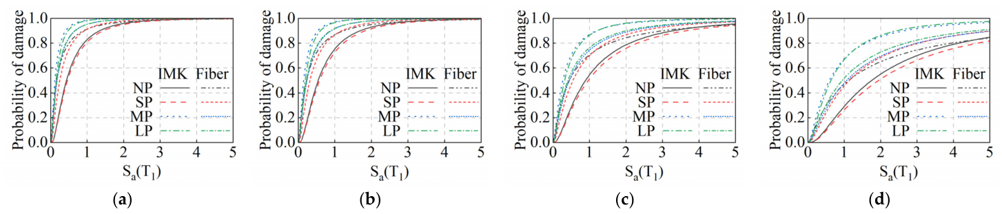
where the symbols denote the seismic demand, the capacity associated with the kth damage state, and the selected ground-motion intensity measure. Peak ground acceleration (PGA) was adopted as the intensity measure, providing a consistent scaling basis for the four ground-motion groups described in Section 5.2 [47]. PGA remained the baseline intensity measure, while an S_a(T₁)-based sensitivity assessment is presented in Section 5.6.

The maximum displacement ductility demand was selected as the engineering demand parameter, consistent with the experimental fragility definition adopted for the prototype RC solid piers [47]:

$${\mathsf{\mu }}_d={\displaystyle \frac{\underset{t}{\max }\left|{\mathsf{\Delta }}_{\mathrm{top}}\left(t\right)\right|}{{\mathsf{\Delta }}_y}}$$

(36)

where ${\mathsf{\Delta }}_{\mathrm{top}}\left(t\right)$ is the pier-top displacement response and ${\mathsf{\Delta }}_y$ is the reference yield displacement. The yield displacement was obtained from the full-scale quasi-static backbone response presented in Section 4.2. The same ${\mathsf{\Delta }}_y$ was applied to both models, ensuring that differences in displacement ductility reflected differences in predicted seismic demand rather than model-specific normalization.

For each ground-motion group and numerical model, the relationship between the median seismic demand and PGA was represented using the conventional power-law probabilistic seismic demand model [49,51]:

$$S_D\left(\mathrm{IM}\right)=a{\left(\mathrm{IM}\right)}^b$$

(37)

where $S_D$ is the median displacement ductility demand, while $a$ and $b$ are regression coefficients. Taking the natural logarithm gives

$$\ln {\mathsf{\mu }}_{d,i}=\ln a+b\ln \mathrm{PG}{\mathrm{A}}_{\mathrm{i}}+{\mathsf{\epsilon }}_i,$$

(38)

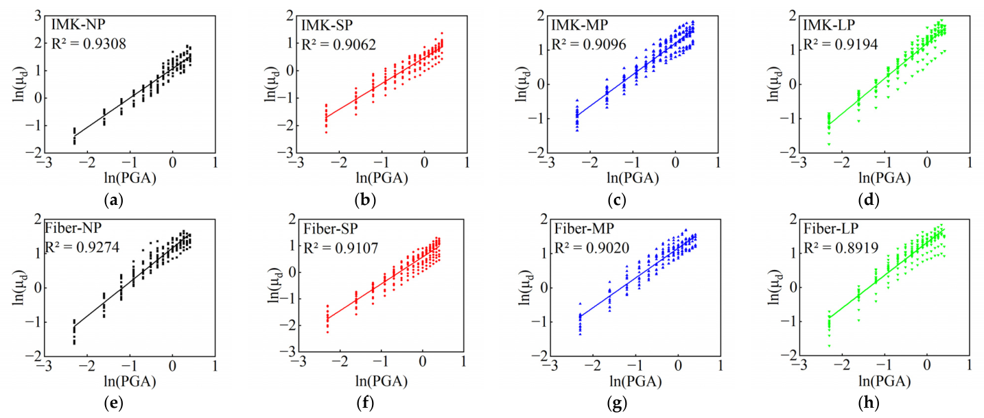
where the symbols denote the displacement ductility demand and intensity measure for the ith analysis case. The regression residual was assumed to follow a normal distribution with zero mean and constant variance. Only successfully resolved cases with finite responses were included in the strict PSDM regressions. Numerical-failure cases were excluded, while drift-limit cases were treated as physical-collapse exceedances rather than as ordinary regression observations [48,50].

The conditional logarithmic dispersion of the seismic demand was calculated as

$${\beta }_{D|\mathrm{I}\mathrm{M}}=\sqrt{{\displaystyle \frac{{\displaystyle {\sum }_{i=1}^N}{[\mathrm{l}\mathrm{n}{\mu }_{d,i}-\mathrm{l}\mathrm{n}(a{{\mathrm{P}\mathrm{G}\mathrm{A}}_i}^b\left)\right]}^2}{N-2}}},$$

(39)

where N is the number of nonlinear dynamic analysis results included in the PSDM. The coefficient of determination, R², was used to evaluate the adequacy of the log-linear regression.

Following the conventional analytical fragility framework, seismic demand and damage-state capacity were assumed to follow lognormal distributions and to be statistically independent. The logarithmic capacity dispersion for the kth damage state was obtained from its coefficient of variation, as follows [48,49]:

$${\mathsf{\beta }}_{C,k}=\sqrt{\ln \left(1+\mathrm{CO}{\mathrm{V}}_{\mathrm{C},\mathrm{k}}^2\right)}.$$

(40)

Accordingly, the probability of exceeding the $k$th damage state at a specified PGA is expressed as

$$P_{f,k}(\mathrm{PGA})=\mathsf{\Phi }[{\displaystyle \frac{\mathrm{l}\mathrm{n}\left(a{\mathrm{P}\mathrm{G}\mathrm{A}}^b\right)-\mathrm{l}\mathrm{n}{S}_{C,k}}{\sqrt{{{\beta }_{D|\mathrm{I}\mathrm{M}}}^2+{{\beta }_{C,k}}^2}}}],$$

(41)

where $S_{C,k}$ is the median displacement ductility capacity associated with the $k$th damage state. The function $\mathsf{\Phi }\left(\cdot \right)$ denotes the cumulative distribution function of the standard normal distribution. The damage-state capacities and corresponding uncertainties are defined in Section 5.3.

The fragility function can also be expressed in the following conventional lognormal form [49]:

$$P_{f,k}\left(\mathrm{PGA}\right)=\mathsf{\Phi }\left[{\displaystyle \frac{\ln \left(\mathrm{PGA}/{\mathsf{\theta }}_k\right)}{{\mathsf{\beta }}_{\mathrm{IM},k}}}\right],$$

(42)

where ${\mathsf{\theta }}_k$ is the median PGA capacity and ${\mathsf{\beta }}_{\mathrm{IM},k}$ is the total logarithmic dispersion expressed in the intensity-measure domain:

$${\beta }_{\mathrm{I}\mathrm{M},k}={\displaystyle \frac{\sqrt{{{\beta }_{D|\mathrm{I}\mathrm{M}}}^2+{{\beta }_{C,k}}^2}}{b}}.$$

(43)

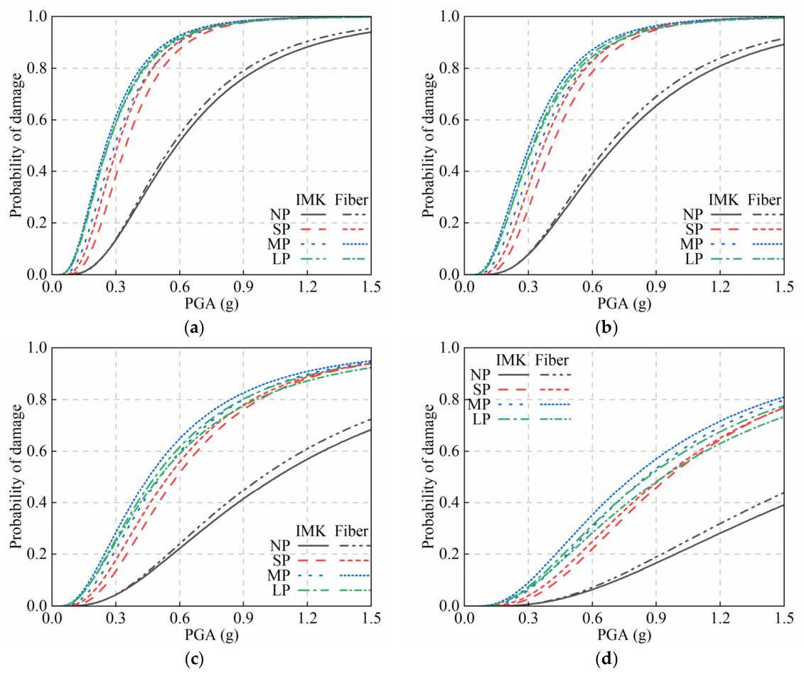
Separate PSDMs and fragility curves were developed for the Fiber and IMK models within each ground-motion group. The model type was treated as a deterministic alternative rather than an additional source of random uncertainty. Therefore, no pooled model-form dispersion was introduced into the fragility functions.

For each IDA case, the maximum pier-top displacement predicted by the IMK model was paired with the corresponding Fiber-model result. Computational time was also recorded under identical hardware, solver, and convergence settings. These paired results provided the basis for evaluating demand-prediction errors, fragility-curve deviations, and the computational efficiency of the simplified IMK model.

5.2. Selection and Scaling of Ground Motions

Near-fault ground motions may contain pronounced velocity pulses that concentrate seismic input within a limited duration and period range. Bridge response can therefore be associated with both ground-motion intensity and the relation between pulse period and structural period. To examine group-dependent associations with this relative-period measure, 60 horizontal records were classified as non-pulse (NP), short-period pulse-like (SP), medium-period pulse-like (MP), or long-period pulse-like (LP), with 15 records per group. Pulse-like records and pulse periods were identified using the wavelet-based procedures of Baker and Shahi [52,53]. Because classification by pulse period does not control all other record properties, it does not by itself isolate a causal pulse-period effect.

Ground-motion records were primarily selected from the PEER NGA-West2 database. The preliminary search used moment magnitudes of 5.0–8.0, rupture distances of 0–30 km, and time-averaged shear-wave velocities in the upper 30 m of 180–760 m/s. Candidate 5% damped acceleration spectra were checked against the target design spectrum over the period range relevant to the bridge. For the selected records, Mw ranged from 5.4 to 7.62, Rrup from 0.27 to 29.74 km, and VS30 from 203.22 to 723.95 m/s. This screening provided broad target-spectrum compatibility, but the four groups were not matched to identical mean spectra or identical S_a(T₁) and PGV distributions. Intergroup spectral and velocity differences therefore remain potential contributors to the response ranking.

For the pulse-like records, the relative pulse-to-structure period ratio was defined as

$$R_T={\displaystyle \frac{T_p}{T_1}},$$

(44)

where $T_p$ denotes the pulse period and $T_1$ is the fundamental period of the complete bridge system. As determined from the modal analysis presented in Section 4.1, the fundamental period was $T_1=1.296\hspace{0.17em}\mathrm{s}$. No dominant velocity pulse was identified for the NP records; therefore, $T_p$ and $R_T$ were not assigned to this group.

As summarized in

Table 8. Pulse-period characteristics of the selected ground-motion groups.

Ground-Motion Group	Abbreviation	Number of Records	${\mathit{T}}_{\mathit{p}}$ Range (Mean), s	${\mathit{R}}_{\mathit{T}}$ Range (Mean)	Relative-Period Characteristic
Non-pulse motions	NP	15	N/A	N/A	No dominant velocity pulse
Short-period pulse-like motions	SP	15	0.518–0.931 (0.745)	0.400–0.719 (0.576)	Pulse period shorter than $T_1$
Medium-period pulse-like motions	MP	15	1.127–1.806 (1.468)	0.870–1.395 (1.134)	Pulse period close to $T_1$
Long-period pulse-like motions	LP	15	1.967–3.773 (2.640)	1.519–2.914 (2.038)	Pulse period substantially longer than $T_1$

, the SP records had $T_p$ values ranging from 0.518 to 0.931 s, with a mean of 0.745 s. Their corresponding $R_T$ values ranged from 0.400 to 0.719, with a mean of 0.576. These records represent motions with pulse periods shorter than the fundamental period of the bridge. For the MP group, $T_p$ ranged from 1.127 to 1.806 s, with a mean of 1.468 s, while $R_T$ ranged from 0.870 to 1.395, with a mean of 1.134. This group represents pulse periods close to $T_1$ and was used to examine possible pulse-to-structure period proximity effects. The LP records had $T_p$ values ranging from 1.967 to 3.773 s, with a mean of 2.640 s. Their $R_T$ values ranged from 1.519 to 2.914, with a mean of 2.038, representing pulse periods substantially longer than $T_1$.

The NP group provides a non-pulse comparison set, whereas the SP, MP, and LP groups represent progressively increasing pulse periods relative to the bridge fundamental period. This classification organizes the analyses by pulse-period category [54,55], but it does not isolate T_p/T₁ from spectral amplitude, PGV, duration, or other record characteristics. The following comparisons are therefore interpreted as group-dependent associations for the selected records.

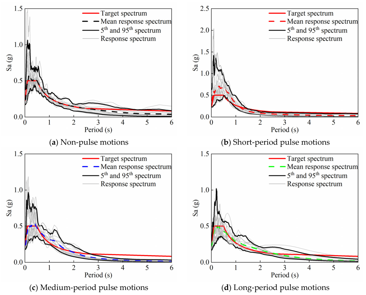
Figure 16 presents the acceleration response spectra of the four record groups [56]. The visible differences among their spectral distributions confirm that the groups differ in more than their pulse period. Applying the same 60 records and PGA levels to both numerical models isolates differences between the Fiber and IMK predictions for a given input. It does not, however, isolate a causal pulse-period effect in comparisons among the NP, SP, MP, and LP groups.

To quantify the intergroup spectral and velocity differences, all 60 records were normalized to PGA = 1.0 g, consistent with Figure 16. Each group contained 15 records, and Sa(T1) was evaluated at T1 = 1.296 s. For NP, SP, MP, and LP, the mean (standard deviation) values of Sa(T1) were 0.849 (0.279), 0.619 (0.380), 1.286 (0.721), and 1.048 (0.433) g, respectively. The corresponding COVs were 0.329, 0.614, 0.560, and 0.413, while their βln Sa values were 0.399, 0.609, 0.523, and 0.528.

For the same NP, SP, MP, and LP groups, the mean (standard deviation) PGV values were 108.08 (36.01), 90.01 (28.75), 125.56 (45.82), and 129.81 (29.16) cm/s, respectively. The corresponding COVs were 0.333, 0.319, 0.365, and 0.225, while their βln PGV values were 0.343, 0.343, 0.399, and 0.263. The MP group had the highest mean Sa(T1), whereas the LP group had the highest mean PGV. These differences confirm that the group-dependent response ranking reflects combined associations with Tp/T1, spectral amplitude, and velocity content rather than the pulse-period ratio alone.

5.3. Damage Measures and Limit-State Definitions

Four cumulative damage limit states were defined to quantify the seismic performance of the full-scale RC solid pier. The four limit states were denoted as slight damage (DS1), moderate damage (DS2), severe damage (DS3), and collapse damage (DS4) [57]. The operational descriptions follow the bridge damage terminology in Hazus [58].

The maximum pier-top displacement ductility, ${\mathsf{\mu }}_d$, defined in Section 5.1, was adopted as the engineering demand parameter for identifying the damage states. The $k$th limit state was considered to be exceeded when

$${\mathsf{\mu }}_d\ge S_{C,k},$$

(45)

The four median displacement-ductility capacities were determined by combining the damage progression observed in the quasi-static tests with Hazus performance descriptions and the relevant literature, as previously reported in Ref. [47]. The adopted values were 1.00, 1.20, 1.76, and 4.76 for DS1–DS4, respectively. These values therefore represent an experimentally and literature-informed damage classification rather than thresholds obtained from a single specimen. Because ductility is normalized by the yield displacement and the scaled pier preserves the main geometric, reinforcement, and axial-load ratios, the same thresholds were applied to the 12 m analytical pier. This transfer remains a modeling assumption in the absence of independent full-scale test data.

The physical interpretations and quantitative criteria for the four damage states are summarized in

Table 9. Definition of limit states for bridge piers.

Limit State	Bridge Operational Functionality	Seismic Damage State	${\mathbf{S}}_{\mathbf{C}}$	${\mathsf{\beta }}_{\mathfrak{c}}$
Slight damage (DS1)	Fully operational	Minor cracking of cover concrete or initial yielding of longitudinal reinforcement	1	0.246
Moderate damage (DS2)	Operational	Initial formation of local plastic hinges, with visible surface cracks	1.2	0.246
Severe damage (DS3)	Life safety	Full formation of plastic hinges, appearance of wide cracks, and extensive spalling of concrete	1.76	0.472
Collapse (DS4)	Near collapse	Severe strength degradation, extensive yielding of longitudinal reinforcement, and crushing of core concrete	4.76	0.472

. DS1 represents the onset of structural damage, characterized primarily by minor flexural cracking of the cover concrete or initial yielding of the longitudinal reinforcement. DS2 corresponds to the initial formation of a localized plastic hinge, accompanied by visible flexural cracks and limited concrete spalling. At DS3, the plastic hinge is fully developed, with wide cracks, extensive cover-concrete spalling, and pronounced inelastic deformation. DS4 represents a near-collapse condition involving severe strength degradation, extensive yielding of the longitudinal reinforcement, crushing of the confined core concrete, and an impending loss of lateral-load resistance.

The displacement-ductility capacities were assumed to follow lognormal distributions. Following the adopted bridge-fragility framework, coefficients of variation of 0.25 were assigned to DS1 and DS2 and 0.50 to DS3 and DS4, reflecting greater uncertainty in severe and near-collapse states [47,59]. These dispersions were retained for the scaled analytical pier; therefore, the absolute fragility estimates remain conditional on the adopted capacity model. The influence of alternative capacity dispersions is examined in Section 5.6.

$${\mathsf{\beta }}_{C,k}=\sqrt{\ln \left(1+\mathrm{CO}{\mathrm{V}}_{\mathrm{k}}^2\right)},$$

(46)

resulting in ${\mathsf{\beta }}_{C,k}=0.246$ for DS1 and DS2 and ${\mathsf{\beta }}_{C,k}=0.472$ for DS3 and DS4.

Identical median capacities and dispersions were used for the Fiber and IMK models. This common capacity model enables a controlled comparison in which differences between paired fragility curves primarily reflect their simulated demands. It does not remove uncertainty in the transferred damage thresholds or demonstrate that those capacities are scale-independent. Because the four limit states are cumulative, their exceedance probabilities at a given PGA should satisfy Equation (47).

$$P\left(\mathrm{DS}1∣\mathrm{PGA}\right)\ge P\left(\mathrm{DS}2∣\mathrm{PGA}\right)\ge P\left(\mathrm{DS}3∣\mathrm{PGA}\right)\ge P\left(\mathrm{DS}4∣\mathrm{PGA}\right).$$

(47)

This unified limit-state framework enables a direct and consistent comparison of the seismic fragility estimates obtained using the detailed Fiber model and the simplified IMK model.

5.4. IDA Results, Model Discrepancy, and Computational Efficiency

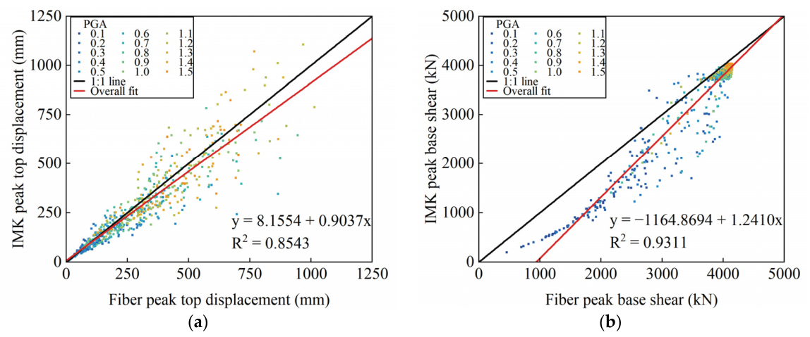
Incremental dynamic analyses were performed using 60 ground-motion records following the IDA framework [50]. Each record was scaled from 0.1 to 1.5 g at 0.1 g increments, giving 15 intensity levels, 900 analyses per model, and 1800 analyses in total. The external wall-clock time was used to evaluate computational efficiency, and the speed-up factor was defined as

$$S_t={\displaystyle \frac{t_{\mathrm{F}\mathrm{i}\mathrm{b}\mathrm{e}\mathrm{r}}}{t_{\mathrm{I}\mathrm{M}\mathrm{K}}}}$$

(48)

where $t_{\mathrm{F}\mathrm{i}\mathrm{b}\mathrm{e}\mathrm{r}}$ and $t_{\mathrm{I}\mathrm{M}\mathrm{K}}$ are the accumulated external wall-clock times required by the Fiber and IMK models, respectively.

Each IDA case was initially analyzed using the Newton algorithm and the Newmark average-acceleration method. When convergence was not achieved, NewtonLineSearch, ModifiedNewton with the initial tangent, and KrylovNewton were attempted sequentially with increased iteration limits and a relaxed convergence tolerance. The analysis time step was then reduced by successive halving to a minimum of 1/128 of the nominal time step. A case was classified as a numerical failure only when all recovery attempts were unsuccessful or a non-finite response was detected.

Of the 900 Fiber analyses, 815 completed the full time history, 14 reached the 10% absolute pier-top drift limit, and 71 failed numerically. Of the 900 IMK analyses, 856 produced successful terminal outcomes, including 15 cases stopped at the 10% drift limit; the remaining 44 cases failed numerically. Thus, 841 IMK cases completed the full time history. The DS4 threshold did not terminate any analysis. Each response history continued unless the 10% drift limit was reached. Drift-limit cases were recorded as physical-collapse observations and retained as collapse exceedances in the revised fragility assessment, whereas numerical failures were excluded from the strict PSDM regressions.

As summarized in

Table 10. Computational costs of the IDA analyses using the Fiber and IMK models.

Model	Number of Analyses	Total Wall-Clock Time (s)	Total Wall-Clock Time (h)	Mean Time per Analysis (s)	Relative Speed-up
Fiber	900	24,574.832	6.826	27.305	1.00
IMK	900	891.925	0.248	0.991	27.55
Total	1800	—	—	—	—

, the Fiber model required a total of 24,574.832 s, equivalent to 6.826 h, whereas the IMK model required only 891.925 s, or approximately 0.248 h. The mean computational times per analysis were 27.305 and 0.991 s for the Fiber and IMK models, respectively. The overall speed-up factor was therefore 27.55, corresponding to a 96.37% reduction in computational time. This substantial improvement indicates that the simplified IMK model is more suitable for large-scale IDA calculations involving numerous ground motions and intensity levels.

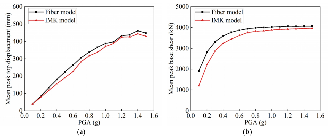
To investigate the development of the seismic response with increasing ground-motion intensity, the mean peak pier-top displacement and mean peak base shear were calculated at each PGA level using paired results from the two models. The corresponding mean responses were defined as

$${\overline{D}}_{\mathrm{m}\mathrm{a}\mathrm{x}}(a)={\displaystyle \frac{1}{N_a}}{\displaystyle {\sum }_{i=1}^{N_a}}{D}_{\mathrm{m}\mathrm{a}\mathrm{x},i}(a)$$

(49)

and

$${\overline{V}}_{\mathrm{m}\mathrm{a}\mathrm{x}}(a)={\displaystyle \frac{1}{N_a}}{\displaystyle {\sum }_{i=1}^{N_a}}{V}_{\mathrm{m}\mathrm{a}\mathrm{x},i}(a)$$

(50)

where $a$ denotes the PGA level, $N_a$ is the number of paired samples at that intensity level, and $D_{\left(max,i\right)}$ and $V_{\left(max,i\right)}$ are the peak pier-top displacement and peak base shear of the $i$-th record, respectively.

Figure 17 compares the mean peak responses. Mean displacement increased from approximately 40 mm at 0.1 g to approximately 440 mm at 1.5 g, and the two models predicted consistent overall growth trends.

The IMK model generally produced slightly smaller mean displacement demands than the Fiber model. The difference between the two mean displacement curves was relatively pronounced at intermediate intensity levels, reaching approximately 15% at 0.5–0.6 g. With a further increase in PGA, the difference gradually decreased. For PGA levels of 1.0–1.5 g, the relative difference between the two mean displacement responses was generally within approximately 2–5%. These results indicate that the IMK model reasonably reproduced the overall development of the displacement demand, although greater dispersion was observed for individual records.

The mean peak base shear exhibited a different development pattern. As the PGA increased from 0.1 to approximately 0.6–0.8 g, the mean peak base shear increased rapidly. Beyond this range, its rate of increase decreased markedly, indicating that the lateral resistance of the bridge pier gradually approached a strength plateau. The mean peak base shears predicted by the Fiber and IMK models increased from 1908.4 and 1208.7 kN at 0.1 g to 4069.1 and 3965.0 kN at 1.5 g, respectively. The difference between the models was relatively large at low intensity levels but decreased continuously as the structural response entered the nonlinear range. At 1.5 g, the difference between the mean peak base shears predicted by the two models was only 2.56%. Thus, the IMK model adequately reproduced both the strength plateau and the overall evolution of the lateral-force demand.

To further evaluate record-level agreement, diagonal-error analyses were performed for peak pier-top displacement and peak base shear. As shown in Figure 18, paired results covering PGA levels from 0.1 to 1.5 g were compared. The Fiber-model results are plotted on the horizontal axis and the corresponding IMK-model results on the vertical axis; the 1:1 diagonal represents perfect agreement between the two models.

For the peak pier-top displacement, the regression analysis yielded a coefficient of determination of 0.854, indicating a strong overall correlation between the predictions of the two models. The mean absolute error and root-mean-square error were 50.19 and 81.01 mm, respectively. The mean signed difference was −18.40 mm, indicating that the IMK model exhibited a slight overall tendency to underestimate the peak displacement. The mean absolute percentage error was 15.95%, and 55.39% of the paired samples fell within the ±15% error bounds. As shown in Figure 18a, the scatter increased with displacement demand, suggesting that the prediction of record-specific deformation demands became more sensitive to the characteristics of the input ground motions at higher response levels.

For the peak base shear, the coefficient of determination increased to 0.931, demonstrating closer agreement between the two models than that obtained for the peak displacement. The mean absolute error and root-mean-square error were 304.65 and 443.84 kN, respectively, while the mean signed difference was −292.88 kN. The corresponding mean absolute percentage error was 11.32%, and 75.51% of the paired samples were located within the ±15% error bounds. As shown in Figure 18b, the peak-base-shear results were more concentrated around the 1:1 line and the fitted regression relationship. These results demonstrate that the simplified IMK model reproduced the global lateral-force demand more consistently than the record-specific peak deformation demand.

Overall, the IDA results demonstrate that the IMK model reproduced the principal development trends in the peak pier-top displacement and peak base shear predicted by the Fiber model. The agreement was particularly strong for the peak lateral-force response, whereas greater record-to-record dispersion was observed in the peak displacement response. Meanwhile, the IMK model reduced the total computational time by more than 96%. Therefore, the combination of reasonable prediction accuracy and high computational efficiency supports the application of the simplified IMK model to large-sample seismic-demand and fragility analyses.

5.5. Fragility Assessment Under Pulse-like Ground Motions

The IDA results presented in Section 5.4 were used to establish probabilistic seismic demand models. PGA was retained as the intensity measure because it was the record-scaling variable and preserves comparability with the adopted fragility framework [49,51]. PGA is not assumed to be the most efficient or sufficient predictor for this period-sensitive problem. A spectral measure such as S_a(T₁) was therefore adopted for the sensitivity assessment in Section 5.6, while PGV was retained for future investigation. Displacement ductility demand was calculated using the common yield displacement defined in Section 5.3.

For each numerical model and ground-motion group, the relationship between displacement ductility demand and PGA was expressed as

$$ln\left({\mu }_d\right)=\alpha +bln\left(PGA\right)+\epsilon$$

(51)

where $\alpha$ and $b$ are the regression coefficients, and $\epsilon$ represents the regression residual. Separate regressions were performed for the NP, SP, MP, and LP groups. This procedure produced eight regression relationships for the two numerical models.

Figure 19 and

Table 11. Parameters of the log-linear probabilistic seismic demand models.

Numerical Model	Ground-Motion Group	α	b	${\mathit{R}}^2$	${\mathit{\beta }}_{\mathit{D}|\mathit{I}\mathit{M}}$	pquad	pBP
IMK	NP	1.0838	1.0711	0.9308	0.240	0.46	0.08
IMK	SP	0.4835	0.9449	0.9062	0.222	0.56	0.11
IMK	MP	1.2071	0.9175	0.9096	0.238	0.09	0.25
IMK	LP	1.2095	1.0313	0.9194	0.223	0.37	0.82
Fiber	NP	1.1697	0.9953	0.9274	0.240	0.50	0.12
Fiber	SP	0.5801	1.0096	0.9107	0.212	0.68	0.94
Fiber	MP	1.1613	0.8691	0.9020	0.253	0.46	0.09
Fiber	LP	1.3254	0.9631	0.8919	0.218	0.07	0.72

Note: The probabilistic seismic demand model is expressed as $\ln \left({\mathsf{\mu }}_d\right)=\mathsf{\alpha }+b\ln \left(\mathrm{PGA}\right)$, where ${\mathsf{\mu }}_d$ is the displacement-ductility demand, $\mathsf{\alpha }$ is the regression intercept, and b is the regression slope. NP, SP, MP, and LP denote non-pulse, short-period pulse, medium-period pulse, and long-period pulse ground-motion groups, respectively. Here, p_quad is the p-value of the quadratic term in the augmented log-demand regression, and p_BP is the p-value of the Breusch–Pagan test. A value greater than 0.05 means that the corresponding null hypothesis was not rejected at the 5% significance level.

present the log-linear regressions and the corresponding conditional logarithmic dispersions, βD|IM, defined as the standard deviations of the regression residuals. All coefficients of determination, R², exceed 0.89, indicating a strong overall association between PGA and displacement ductility demand within the fitted range. The βD|IM values range from 0.212 to 0.253 across the eight regressions, indicating moderate and broadly comparable residual scatter. Because R² alone does not verify the assumed functional form or constant conditional variance, two supplementary diagnostics were performed for each model–group regression. Log-linearity was assessed by adding [ln(PGA)]² to the regression and testing the quadratic-term coefficient, while homoscedasticity was assessed using the Breusch–Pagan test. As summarized in Table 11, the quadratic-term p-values range from 0.07 to 0.68 and the Breusch–Pagan p-values range from 0.08 to 0.94. At the 5% significance level, neither test rejects log-linearity or constant conditional variance for any of the eight demand models. These results provide no statistically significant evidence of curvature or heteroscedasticity over 0.1–1.5 g, although they support, rather than prove, the adequacy of the adopted first-order log-linear approximation.

The demand models were combined with the limit states defined in Section 5.3 to calculate exceedance probabilities. Figure 20 compares the fragility curves predicted by the Fiber and IMK models for DS1–DS4.

The median PGA capacities and corresponding total logarithmic dispersions are summarized in

Table 12. Median PGA capacities and total logarithmic dispersions of the fragility models.

Numerical Model	Ground-Motion Group	θDS1 (g)	θDS2 (g)	θDS3 (g)	θDS4 (g)	βIM, DS1–DS2	βIM, DS3–DS4
IMK	NP	0.5995	0.7270	1.0904	1.9174	0.3630	0.5602
IMK	SP	0.3636	0.4310	0.6163	1.0139	0.3160	0.4915
IMK	MP	0.3095	0.3694	0.5355	0.8981	0.3350	0.5148
IMK	LP	0.2683	0.3273	0.4968	0.8885	0.3641	0.5706
Fiber	NP	0.5629	0.6744	0.9855	1.6713	0.3403	0.5246
Fiber	SP	0.3088	0.3708	0.5449	0.9311	0.3264	0.5201
Fiber	MP	0.2526	0.3052	0.4542	0.7902	0.3666	0.5564
Fiber	LP	0.2628	0.3242	0.5037	0.9304	0.3788	0.5989

Note: θDSk denotes the median PGA capacity for damage state DSk, and βIM denotes the corresponding total logarithmic dispersion in the intensity-measure domain. DS1–DS2 and DS3–DS4 share the adopted capacity-dispersion levels.

.

As shown in Figure 20, the exceedance probability increased continuously with PGA for all damage states. The fragility curves shifted progressively to the right from DS1 to DS4 because higher displacement demands were required to reach more severe damage states. The curve slopes also decreased for DS3 and DS4, reflecting the increased uncertainty associated with extensive damage and collapse.

For the selected records, the SP curves were farthest to the right and had the lowest exceedance probabilities at a given PGA, whereas the MP and LP curves were generally farther to the left and the NP curves were mostly intermediate. Thus, pulse-like classification alone did not correspond to a uniform increase in fragility. The observed ordering is associated with the combined properties of the four selected groups. Because their spectra and velocity characteristics were not matched, this cannot be attributed solely to the pulse-to-structure period ratio.

The representative fundamental period of the bridge was 1.296 s. The MP pulse periods were close to this value, and the MP group exhibited relatively large displacement demands; the LP group also showed considerable fragility, while the SP group showed lower fragility within the investigated PGA range. These coincidences are consistent with a possible pulse-period association, but differences in S_a(T₁), PGV, duration, and other record properties may also contribute. The present group comparison therefore does not establish T_p/T₁ as the sole causal variable.

The Fiber and IMK models produced similar curve shapes and the same group-dependent ordering for the selected records. The MP curves showed the closest agreement, whereas larger differences occurred for several NP and LP curves. The IMK curves were generally shifted slightly to the right for the NP, SP, and LP groups, and therefore predicted slightly lower damage probabilities for those groups.

The differences between the two models were quantified directly from the paired fragility curves. Across the 16 curve pairs, the mean absolute difference in damage exceedance probability was 3.14 percentage points. The curve-specific mean differences ranged from 0.18 to 5.08 percentage points. The largest localized difference over the investigated PGA range was of approximately 14.1 percentage points.

The relative difference in the PGA corresponding to a 50% exceedance probability was also calculated. The mean absolute relative difference between the two models was 11.23%, with individual values ranging from 0.96% to 22.55%. The MP group showed the smallest average difference, confirming the particularly close agreement observed in Figure 20.

At a PGA of 1.0 g, the IMK and Fiber models predicted DS4 exceedance probabilities of 0.491 and 0.544 for the NP group. The corresponding probabilities were 0.191 and 0.233 for the SP group. For the MP group, the probabilities were 0.563 and 0.538, respectively. For the LP group, they were 0.562 and 0.627. Thus, the absolute differences at this intensity ranged from 2.6 to 6.5 percentage points.

Although the IMK model generally predicted slightly lower fragility, this difference was not uniform across all damage states. The IMK model produced slightly higher probabilities for several MP cases. Therefore, the simplified model did not exhibit a consistently conservative or non-conservative bias. All model-to-model differences reported here are conditional on the common PGA-based demand model, transferred capacity distributions, and selected ground-motion groups.

The IDA results in Section 5.4 showed that the IMK model reduced the total computational time by 96.37%. Meanwhile, the mean difference between the paired fragility probabilities was of only 3.14 percentage points. Therefore, the IMK model achieved a favorable balance between prediction accuracy and computational efficiency. It can thus rapidly estimate seismic damage probabilities and facilitate large-scale fragility assessment using extensive ground-motion suites.

5.6. Sensitivity to the Intensity Measure and Capacity Dispersion

To examine the influence of intensity-measure selection, the fragility functions were re-estimated using the 5% damped S_a(T₁), with T₁ = 1.296 s. The displacement-ductility demand, valid-case filtering, damage capacities, and record groups remained unchanged. Only the intensity measure used in the PSDM and fragility calculations was replaced.

The S_a(T₁)-based curves increased monotonically and shifted progressively to the right from DS1 to DS4, as shown in Figure 21. The MP and LP groups generally produced higher exceedance probabilities, whereas the SP group remained comparatively less vulnerable. The paired Fiber and IMK curves also remained close, without a uniform conservative or non-conservative bias. Thus, replacing PGA with S_a(T₁) did not reverse the principal group-dependent ordering or the model-to-model comparison reported in Figure 20. However, this sensitivity check did not isolate the pulse-period effect because PGV, spectral shape, and other record properties still differed among groups.

The influence of damage-capacity uncertainty was examined by varying the adopted coefficients of variation while retaining the median capacities in Table 9. The lower-dispersion scenario used COVs of 0.20 for DS1–DS2 and 0.40 for DS3–DS4. The baseline scenario retained 0.25 and 0.50, while the higher-dispersion scenario used 0.30 and 0.60. For each scenario, the mean absolute probability difference between the paired Fiber and IMK fragility curves was recalculated.

As summarized in

Table 13. Sensitivity of the mean absolute Fiber–IMK fragility difference to damage-capacity dispersion.

Scenario	COV, DS1–DS2	COV, DS3–DS4	Mean |ΔPf|, DS1 (%)	DS2 (%)	DS3 (%)	DS4 (%)	Overall Mean (%)
Lower dispersion	0.20	0.40	2.80	3.11	3.53	3.41	3.21
Baseline	0.25	0.50	2.79	3.09	3.41	3.26	3.14
Higher dispersion	0.30	0.60	2.78	3.07	3.29	3.12	3.07

Note: ΔP_f denotes difference in damage-state exceedance probability between paired IMK and Fiber fragility curves. Probability differences are reported in percentage points, and median capacities were unchanged.

, the overall mean absolute probability difference was of 3.21, 3.14, and 3.07 percentage points for the lower, baseline, and higher dispersion scenarios, respectively. The corresponding variation was only 0.14 percentage points over the investigated range. The Fiber–IMK ordering remained unchanged for all 16 ground-motion-group and damage-state combinations. Increasing capacity dispersion slightly reduced the model-to-model separation for the more severe damage states, but it did not materially alter the comparative fragility conclusions. These findings support the robustness of the Fiber–IMK comparison within the examined capacity-dispersion range, while the absolute fragility estimates remain conditional on the transferred capacity model.

6. Conclusions

This study did not introduce a new hysteretic law or a new experimental database. Rather, it calibrated the established IMK formulation for urban rail RC solid piers and evaluated the resulting simplified representation across the reused seven-specimen dataset, an analytically scaled 12 m prototype, nonlinear dynamics, IDA, computational cost, and PGA-based fragility with intensity-measure and capacity-dispersion sensitivity analyses. The specimen comparisons are calibration-set assessments, and the full-scale Fiber comparisons are internal analytical benchmarks because the IMK backbone was extracted from the same Fiber response. The principal conclusions, interpreted within these boundaries, are as follows:

1. Calibration of the IMK backbone reproduced the measured yield, peak, post-peak, and positive–negative asymmetric strength characteristics of the seven specimens. Additional calibration-set response measures quantified global cyclic accuracy. For final secant stiffness, the IMK model achieved R² = 0.891 and a mean absolute percentage error of 9.93%. For cumulative hysteretic energy, R² reached 0.893, although the mean absolute percentage error was 27.79% and energy was underestimated under high cyclic demands. Residual displacement remained more scattered because of its sensitivity to unloading, pinching, and the final zero-force crossing. These results do not establish out-of-sample predictive capability.

2. The IMK, Fiber, and SAP2000 models produced consistent initial dynamic characteristics for the analytically scaled bridge, with a mean fundamental period of 1.296 s. In the quasi-static Fiber benchmark, the mean force difference at intermediate backbone points was 3.83%. Under the representative dynamic records, the mean relative differences between the IMK and Fiber models were 2.64% for peak base shear and 4.15% for peak pier-top displacement. The IMK model underestimated cumulative energy at the largest quasi-static displacement by 15.39%. Because the IMK backbone was identified from the Fiber response, these comparisons quantify internal consistency and interpolation accuracy rather than independent full-scale validation. For the eight-record damping sensitivity check, replacing the baseline mass-proportional formulation with a one-mode-compatible 5% modal implementation changed the peak displacement and base shear only at the numerical round-off level.

3. Across the full IDA intensity range, the IMK and Fiber predictions remained strongly correlated. The coefficients of determination were 0.854 for peak pier-top displacement and 0.931 for peak base shear, with corresponding mean absolute percentage errors of 15.95% and 11.32%. The simplified model reduced total wall-clock time by 96.37% and achieved an overall speed-up factor of 27.55. These results show that the principal global seismic demands can be estimated with limited error and substantially lower computational effort.

4. Both models reproduced the same group-dependent fragility ordering for the selected records: the SP group had the lowest fragility, whereas the MP and LP groups generally produced larger displacement demands. The mean absolute difference between paired exceedance probabilities was 3.14 percentage points, and the mean relative difference in median PGA capacity was 11.23%. Combined with the 27.55-fold IDA acceleration, this agreement supports rapid comparative fragility and global pier-damage assessment within the adopted PGA-based framework. Because the groups were not matched to identical S_a(T₁), PGV, or spectral distributions, the ordering is reported as an association and is not attributed solely to T_p/T₁. The model bias was not uniformly conservative or non-conservative. Replacing PGA with S_a(T₁) preserved the main ordering and close Fiber–IMK agreement. Across the three capacity-dispersion scenarios, the overall mean probability difference ranged from 3.07 to 3.21 percentage points. The model ordering remained unchanged for all 16 group-damage-state combinations.

Overall, calibration of the existing IMK formulation provides a practical balance between global-response accuracy and computational efficiency for large-sample analyses of urban rail RC solid piers within the investigated domain. Its independent positive- and negative-direction parameters provide an explicit representation of departure from symmetric hysteresis, while the results show where that simplified asymmetry representation is adequate for global response. Fiber or coupled axial–flexure–shear models remain necessary when local shear damage, bond slip, reinforcement strain, residual deformation, detailed energy dissipation, or path-dependent P–Δ behavior governs the decision. Generalization remains limited by reuse of the calibration specimens, the analytically scaled prototype, transferred deterioration and capacity assumptions, the restriction of the damping sensitivity check to one-mode-compatible formulations and eight representative records, the selected PGA and Sa(T1) measures, and unmatched ground-motion spectra. Future studies should use independent specimens or cross-validation, full-scale evidence, alternative multi-mode damping targets and velocity-related intensity measures, broader residual diagnostics, and additional axial-load ratios, section geometries, and loading histories. Future work should also quantify cyclic-parameter sensitivity, parameter interactions, and uncertainty propagation using automated calibration procedures and independent datasets.

References

1. Hu, J.; Wen, W.; Zhai, C.; Pei, S. A Comprehensive Review of Resilience of Urban Metro Systems: A Perspective from Earthquake Engineering. Tunn. Undergr. Space Technol. 2024, 152, 105920. [Google Scholar] [CrossRef] [Scilit]
2. Hu, J.; Wen, W.; Zhai, C.; Pei, S. Post-Earthquake Functionality Assessment for Urban Subway Systems: Incorporating the Combined Effects of Seismic Performance of Structural and Non-Structural Systems and Functional Interdependencies. Reliab. Eng. Syst. Saf. 2024, 241, 109641. [Google Scholar] [CrossRef] [Scilit]
3. Ba, Z.; Sun, Y.; Li, D.; Han, S.; Lu, Y.; Sun, D. Full-Process Seismic Simulation Method for Urban Underground Rail Transit Networks Considering Source-Path-Structure Effects. Tunn. Undergr. Space Technol. 2025, 164, 106780. [Google Scholar] [CrossRef] [Scilit]
4. Aloschi, F.; Di Costanzo, L.; Miano, A.; Pariota, L.; Bifulco, G.N.; Prota, A. A Framework for Resilience Assessment of Urban Transportation Systems under Seismic Hazard. Transp. Res. Interdiscip. Perspect. 2026, 37, 101989. [Google Scholar] [CrossRef] [Scilit]
5. Huang, Y.; Wang, J.; Le, W.; Zhang, L.; Su, J. Study on Mechanical Behaviours of Rail Fasteners and Effects on Seismic Performance of Urban Rail Viaduct. Structures 2021, 33, 3822–3834. [Google Scholar] [CrossRef] [Scilit]
6. Yu, J.; Jiang, L.; Zhou, W.; Lai, Z.; Zuo, Y.; Peng, K. Component Damage and Failure Sequence of Track-Bridge System for High-Speed Railway under Seismic Action. J. Earthq. Eng. 2023, 27, 656–678. [Google Scholar] [CrossRef] [Scilit]
7. Feng, Y.; Xu, S.; Wu, B.; Zhou, W.; Liu, X.; Wu, L.; Rao, J.; Xiang, P.; Guo, Z. Transverse-Direction Post-Seismic Running Safety of Longitudinally Connected Ballastless Track–Continuous Girder Bridge Systems Considering Earthquake Damage State. Buildings 2024, 14, 3803. [Google Scholar] [CrossRef] [Scilit]
8. Zeng, C.; Guo, W.; Jiang, L.; Wang, Y.; Jin, R.; Zhang, S.; Xiao, J.; Sun, Z.; Ma, H.; He, Z.; et al. Seismic Safety of High-Speed Railway Train Track Bridge Systems: Research Progress, Disaster Mechanisms, and Mitigation Strategies. J. Railw. Sci. Technol. 2025, 1, 2–30, Corrigendum in J. Railw. Sci. Technol. 2025, 1, 184. [Google Scholar] [CrossRef] [Scilit]
9. Somala, S.N.; Todorov, B.; Billah, A.H.M.M. Seismic Fragility and Damage Assessment of RC Bridge Pier under Long-Duration, near-Fault, and Far-Field Ground Motions. Structures 2021, 31, 671–685. [Google Scholar] [CrossRef] [Scilit]
10. Duan, L.; Yang, H.; Qi, Q.; Wu, Q.; Shao, C.; Yang, Y. Flexure–Shear Response of a RC Double-Column Bridge Pier: Individual Column Cyclic Tests and System-Level Numerical Analysis. Buildings 2026, 16, 3188. [Google Scholar] [CrossRef] [Scilit]
11. Cui, H.; Shao, C. Experimental Study on Seismic Performance of Circular Hollow Piers with Low-to-Medium Shear-Span Ratio in High-Seismic Intensity Regions. Structures 2026, 87, 111767. [Google Scholar] [CrossRef] [Scilit]
12. Cui, H.; Shao, C. Experimental Investigation on the Flexure-Shear Coupled Deformation Performance of Circular Hollow Piers in Highway Bridges. Structures 2026, 88, 111799. [Google Scholar] [CrossRef] [Scilit]
13. Cui, H.; Shao, C.; Wei, W.; Zhang, Y.; Qi, Q.; Wang, C.; Long, J. Failure Mechanisms and Seismic Damage Control of Variable-Section Round-Ended Hollow Railway Piers in the Transverse Direction. Eng. Fail. Anal. 2026, 193, 110883. [Google Scholar] [CrossRef] [Scilit]
14. Polimeru, V.K.; Laskar, A. CSMM Based Seismic Fragility Analysis of Shear Dominant RC Hollow Rectangular Bridge Piers. Bull. Earthq. Eng. 2021, 19, 5051–5085. [Google Scholar] [CrossRef] [Scilit]
15. Homaei, F. The Probabilistic Performance-Based Seismic Assessment of Concrete Bridge Piers with SMASC Reinforcing Bars: Effect of Pulse-like Ground Motion and Vertical Load-to-Capacity Ratio. Soil Dyn. Earthq. Eng. 2024, 185, 108874. [Google Scholar] [CrossRef] [Scilit]
16. Zhou, Y.; Gao, C.; Yang, S.; Guo, W.; Jiang, L. Seismic Fragility Analysis of Reinforced Concrete Simply Supported Girder Bridges Resting on Double-Column Piers for High Speed Railway. Buildings 2024, 14, 3072. [Google Scholar] [CrossRef] [Scilit]
17. Wang, X.; Li, W.; Liu, Z. Experimental Investigation and Fragility Analysis on Seismic Performance of Precast UHPC Hollow Piers under Varying Axial Load. Soil Dyn. Earthq. Eng. 2025, 196, 109420. [Google Scholar] [CrossRef] [Scilit]
18. Turchetti, F.; Tubaldi, E.; Douglas, J.; Zanini, M.A.; Dall’Asta, A. A Risk-Targeted Approach for the Seismic Design of Bridge Piers. Bull. Earthq. Eng. 2023, 21, 4923–4950. [Google Scholar] [CrossRef] [Scilit]
19. Srivastava, C.; Pandikkadavath, M.S.; Mangalathu, S.; AlHamaydeh, M. Seismic Response of RC Bridges under Near-Fault Ground Motions: A Parametric Investigation. Structures 2024, 61, 106033. [Google Scholar] [CrossRef] [Scilit]
20. Navvar, K.M.; Nadeem, E.; Pandikkadavath, M.S.; Mangalathu, S. Seismic Resilience Assessment of RC Bridge Using System Fragility Based on Maximum and Residual Demand Parameters. Structures 2025, 82, 110791. [Google Scholar] [CrossRef] [Scilit]
21. Al Hawarneh, A.; Alam, M.S. Novel Time-Dependent Seismic Fragility Assessment Tool for Existing RC Highway Bridges in a Multi-Hazard Environment Considering Regular Maintenance. Eng. Struct. 2025, 330, 119868. [Google Scholar] [CrossRef] [Scilit]
22. Al Hawarneh, A.; Alam, M.S.; Pantazopoulou, S.J. Seismic Drift Estimates of Corroded Piers: A Multihazard Approach Utilizing 3D-IDA Analysis with Time Stamps Considering Climate Change Effects. Earthq. Eng. Struct. Dyn. 2025, 54, 1044–1063. [Google Scholar] [CrossRef] [Scilit]
23. Crespi, P.; Scamardo, M.; Buoninconti, R. Fragility Curves for the Seismic Vulnerability of a Stock of Italian Highway Bridges. Structures 2025, 78, 109374. [Google Scholar] [CrossRef] [Scilit]
24. Mao, Y.; He, C.; Jiang, L.; Lai, Z. Seismic Fragility of the Overhead Catenary System on High-Speed Railway Bridges Using Composite Intensity Measure Classification. Structures 2025, 79, 109578. [Google Scholar] [CrossRef] [Scilit]
25. Chirdeep, N.R.; Gangwar, M.; Shekhar, S.; Bahurudeen, A. Seismic Resilience of Deteriorating Bridges under Changing Climatic Conditions. Eng. Struct. 2025, 324, 119355. [Google Scholar] [CrossRef] [Scilit]
26. Wei, B.; Zheng, X.; Jiang, L.; Lai, Z.; Zhang, R.; Chen, J.; Yang, Z. Seismic Response Prediction and Fragility Assessment of High-Speed Railway Bridges Using Machine Learning Technology. Structures 2024, 66, 106845. [Google Scholar] [CrossRef] [Scilit]
27. Rahmat Rabi, R.; Monti, G. Machine Learning-Derived Equations for Seismic Fragility of Hollow-Core Bridge Piers Using Analytical Models and Visible Parameters. Structures 2025, 75, 108792. [Google Scholar] [CrossRef] [Scilit]
28. Dai, J.-C.; Wang, D.-S.; Chen, X.-Y.; Tang, W.-J.; Zhang, R.; Hui, Y.-X. Evaluation of Efficacy of Intensity Measures for Fast and Reliable Seismic Fragility Analysis of Bridge Columns. Soil Dyn. Earthq. Eng. 2025, 198, 109614. [Google Scholar] [CrossRef] [Scilit]
29. Cui, H.; Shao, C.; Wei, W.; Zhang, Y.; Qi, Q.; Long, J. Prediction of Equivalent Damping Ratio for Round-Ended Hollow Railway Bridge Piers with Variable Sections Based on GA-BP Neural Network and Quasi-Static Test. Mech. Syst. Signal Process. 2026, 244, 113810. [Google Scholar] [CrossRef] [Scilit]
30. Cui, H.; Shao, C.; Wei, W.; Zhang, Y.; Qi, Q.; Wang, C. Data-Driven Prediction of Effective Stiffness for Thin-Walled Hollow Piers via a GA-BP Neural Network with Quasi-Static Test Validation. Adv. Eng. Softw. 2026, 218, 104194. [Google Scholar] [CrossRef] [Scilit]
31. Ibarra, L.F.; Medina, R.A.; Krawinkler, H. Hysteretic Models That Incorporate Strength and Stiffness Deterioration. Earthq. Eng. Struct. Dyn. 2005, 34, 1489–1511. [Google Scholar] [CrossRef] [Scilit]
32. Wang, Z.; Wang, J.; Xiu, H.; Liu, T. Hysteretic Model for Reinforced Concrete Rectangular Bridge Columns with Flexure-Shear Failure Mode. China J. Highw. Transp. 2017, 30, 129–138. [Google Scholar]
33. Rahnama, M.; Krawinkler, H. Effects of Soft Soil and Hysteresis Model on Seismic Demands; John, A., Ed.; Blume Earthquake Engineering Center, Stanford University: Stanford, CA, USA, 1993. [Google Scholar]
34. Lignos, D.G.; Krawinkler, H. Deterioration Modeling of Steel Components in Support of Collapse Prediction of Steel Moment Frames under Earthquake Loading. J. Struct. Eng. 2011, 137, 1291–1302. [Google Scholar] [CrossRef] [Scilit]
35. Park, R. Evaluation of Ductility of Structures and Structural Assemblages from Laboratory Testing. Bull. N. Z. Natl. Soc. Earthq. Eng. 1989, 22, 155–166. [Google Scholar] [CrossRef] [Scilit]
36. Ministry of Transport of the People’s Republic of China. Specifications for Seismic Design of Highway Bridges; Ministry of Transport of the People’s Republic of China: Beijing, China, 2020.
37. Wibowo, A.; Wilson, J.L.; Lam, N.T.K.; Gad, E.F. Drift Performance of Lightly Reinforced Concrete Columns. Eng. Struct. 2014, 59, 522–535. [Google Scholar] [CrossRef] [Scilit]
38. Mander, J.B.; Priestley, M.J.N.; Park, R. Theoretical Stress-Strain Model for Confined Concrete. J. Struct. Eng. 1988, 114, 1804–1826. [Google Scholar] [CrossRef] [Scilit]
39. LeBorgne, M.R.; Ghannoum, W.M. Analytical Element for Simulating Lateral-Strength Degradation in Reinforced Concrete Columns and Other Frame Members. J. Struct. Eng. 2014, 140, 04014038. [Google Scholar] [CrossRef] [Scilit]
40. Spacone, E.; Filippou, F.C.; Taucer, F.F. FIBRE BEAM-COLUMN MODEL FOR NON-LINEAR ANALYSIS OF R/C FRAMES: PART I. FORMULATION. Earthq. Eng. Struct. Dyn. 1996, 25, 711–725. [Google Scholar] [CrossRef] [Scilit]
41. McKenna, F. OpenSees: A Framework for Earthquake Engineering Simulation. Comput. Sci. Eng. 2011, 13, 58–66. [Google Scholar] [CrossRef] [Scilit]
42. Kunnath, S.K.; Heo, Y.; Mohle, J.F. Nonlinear Uniaxial Material Model for Reinforcing Steel Bars. J. Struct. Eng. 2009, 135, 335–343. [Google Scholar] [CrossRef] [Scilit]
43. Zhao, J.; Sritharan, S. Modeling of Strain Penetration Effects in Fiber-Based Analysis of Reinforced Concrete Structures. ACI Struct. J. 2007, 104, 133–141. [Google Scholar] [CrossRef] [Scilit]
44. Bouazza, H.; Djelil, M.; Matallah, M. On the Relevance of Incorporating Bar Slip, Bar Buckling and Low-Cycle Fatigue Effects in Seismic Fragility Assessment of RC Bridge Piers. Eng. Struct. 2022, 256, 114032. [Google Scholar] [CrossRef] [Scilit]
45. Qi, Q.; Shao, C.; Yang, H.; Cui, H.; Chen, Z.; Gong, W. Axial-Flexure-Shear Model for Seismic Analysis of RC Thin-Walled Hollow Piers. Soil Dyn. Earthq. Eng. 2025, 195, 109375. [Google Scholar] [CrossRef] [Scilit]
46. Qi, Q.; Jiang, L.; Shao, C.; Yang, H.; Shao, J.; Zhou, Y.; Cui, H. Hysteretic Behavior Modeling of RC Walls Considering Axial-Flexure-Shear Interaction. J. Build. Eng. 2025, 111, 113628. [Google Scholar] [CrossRef] [Scilit]
47. Duan, L.; Yang, H.; Qi, Q.; Wu, Q.; Shao, C.; Jiang, L. Seismic Fragility of Urban Rail Transport RC Solid Piers Considering Multiparameter Effects. Buildings 2026, 16, 2327. [Google Scholar] [CrossRef] [Scilit]
48. Cornell, C.A.; Jalayer, F.; Hamburger, R.O.; Foutch, D.A. Probabilistic Basis for 2000 SAC Federal Emergency Management Agency Steel Moment Frame Guidelines. J. Struct. Eng. 2002, 128, 526–533. [Google Scholar] [CrossRef] [Scilit]
49. Baker, J.W. Efficient Analytical Fragility Function Fitting Using Dynamic Structural Analysis. Earthq. Spectra 2015, 31, 579–599. [Google Scholar] [CrossRef] [Scilit]
50. Vamvatsikos, D.; Cornell, C.A. Incremental Dynamic Analysis. Earthq. Eng. Struct. Dyn. 2001, 31, 491–514. [Google Scholar] [CrossRef] [Scilit]
51. Zhong, J.; Gardoni, P.; Rosowsky, D.; Haukaas, T. Probabilistic Seismic Demand Models and Fragility Estimates for Reinforced Concrete Bridges with Two-Column Bents. J. Eng. Mech. 2008, 134, 495–504. [Google Scholar] [CrossRef] [Scilit]
52. Baker, J.W. Quantitative Classification of Near-Fault Ground Motions Using Wavelet Analysis. Bull. Seismol. Soc. Am. 2007, 97, 1486–1501. [Google Scholar] [CrossRef] [Scilit]
53. Shahi, S.K.; Baker, J.W. An Efficient Algorithm to Identify Strong-Velocity Pulses in Multicomponent Ground Motions. Bull. Seismol. Soc. Am. 2014, 104, 2456–2466, Erratum in Bull. Seismol. Soc. Am. 2019, 109, 2767. [Google Scholar] [CrossRef] [Scilit]
54. Yang, T.; Wei, Y.; Zhong, J. Potential Bias of Conventional Structural Seismic Fragility for Bridge Structures under Pulse-like Ground Motions: Bias Evaluation and Strategy Improvement. Soil Dyn. Earthq. Eng. 2023, 166, 107787. [Google Scholar] [CrossRef] [Scilit]
55. Jiang, L.; Duan, H.; Wen, T.; Jiang, L. Effects of Near-Fault Pulse-Like Ground Motions and Pulse Parameters on a High-Speed Railway Long-Span Arch Bridge–Track System. J. Bridge Eng. 2025, 30, 04024112. [Google Scholar] [CrossRef] [Scilit]
56. Qi, Q.; Zhou, H.; Yang, H.; Chen, X.; Chen, L.; Shao, C.; Cui, H. Seismic Responses of an FPB-Isolated Railway Continuous Beam Bridge under Pulse-Type Motions: Shaking Table Tests and Simulations. Soil Dyn. Earthq. Eng. 2026, 209, 110506. [Google Scholar] [CrossRef] [Scilit]
57. Duan, L.; Yang, H.; Qi, Q.; Wu, Q.; Shao, C.; Yang, Y. Seismic Response and Fragility of Rectangular RC Hollow Tall Piers Under Near-Fault Ground Motions Considering Flexure–Shear Interaction. Symmetry 2026, 18, 1421. [Google Scholar] [CrossRef] [Scilit]
58. Federal Emergency Management Agency. Hazus Earthquake Model Technical Manual, Version 6.1; Federal Emergency Management Agency: Washington, DC, USA, 2024.
59. Miano, A.; Iacovazzo, P.; Mele, A.; Di Ludovico, M.; Prota, A. Seismic Fragility of Circular Piers in Simply Supported RC Bridges: A Proposal for Capacity Assessment. Eng. Struct. 2024, 302, 117426. [Google Scholar] [CrossRef] [Scilit]
Figure 1. Backbone curve of the IMK hysteretic model.
Symmetry 18 01493 g001
Figure 2. Pinching rules of the IMK hysteretic model: (a) two-stage reloading through the pinching control point; (b) direct reloading after a relatively large residual deformation.
Symmetry 18 01493 g002
Figure 3. Cyclic deterioration rules of the IMK hysteretic model: (a) basic strength deterioration; (b) post-capping strength deterioration; (c) unloading stiffness deterioration; and (d) accelerated reloading deterioration.
Symmetry 18 01493 g003
Figure 4. Definition of the equivalent yield point using the Park method.
Symmetry 18 01493 g004
Figure 5. Modeling strategy.
Symmetry 18 01493 g005
Figure 6. Prototype bridge and quarter-scale pier specimen: (a) prototype bridge; (b) specimen details.
Symmetry 18 01493 g006
Figure 7. Quasi-static cyclic test setup and instrumentation arrangement: (a) schematic of the loading system; (b) photograph of the experimental setup.
Symmetry 18 01493 g007
Figure 8. Experimental backbone curves of the seven RC solid-pier specimens.
Symmetry 18 01493 g008
Figure 9. Comparison of the experimental, Fiber-model, and IMK-model hysteretic responses: (a) A1; (b) A2; (c) A3; (d) B1; (e) B2; (f) C1; and (g) C2.
Symmetry 18 01493 g009
Figure 10. Cumulative normalized hysteretic energy obtained from the experimental, Fiber-model, and IMK-model responses: (a) A1; (b) A2; (c) A3; (d) B1; (e) B2; (f) C1; and (g) C2.
Symmetry 18 01493 g010
Figure 11. Diagonal-error comparisons between the experimental and numerical results for the seven specimens: (a) residual displacement; (b) cumulative hysteretic energy; and (c) secant stiffness.
Symmetry 18 01493 g011
Figure 12. Comparison of the quasi-static cyclic responses of the full-scale pier obtained using the Fiber and IMK models.
Symmetry 18 01493 g012
Figure 13. Eight representative ground motions scaled to PGA = 1.0 g: (a) 5% damped acceleration response spectra, and (b) acceleration time histories.
Symmetry 18 01493 g013
Figure 14. Comparison of the dynamic hysteretic responses predicted by the Fiber and IMK models at PGA = 1.0 g: (a) NP-RSN4111; (b) NP-RSN725; (c) SP-RSN1052; (d) SP-RSN568; (e) MP-RSN150; (f) MP-RSN4847; (g) LP-RSN4458; and (h) LP-RSN3746.
Symmetry 18 01493 g014
Figure 15. Comparison of the pier-top displacement histories predicted by the Fiber and IMK models at PGA = 1.0 g: (a) NP-RSN4111; (b) NP-RSN725; (c) SP-RSN1052; (d) SP-RSN568; (e) MP-RSN150; (f) MP-RSN4847; (g) LP-RSN4458; and (h) LP-RSN3746.
Symmetry 18 01493 g015
Figure 16. Acceleration response spectra of the selected ground-motion sets: (a) NP; (b) SP; (c) MP; and (d) LP.
Symmetry 18 01493 g016
Figure 17. Variations in the mean peak responses with increasing PGA predicted by the Fiber and IMK models: (a) mean peak pier-top displacement, and (b) mean peak base shear.
Symmetry 18 01493 g017
Figure 18. Record-level diagonal-error comparisons between the Fiber and IMK models over the PGA range of 0.1–1.5 g: (a) peak pier-top displacement, and (b) peak base shear.
Symmetry 18 01493 g018
Figure 19. Log-linear regressions between displacement ductility demand and PGA for the four ground-motion groups: (ad) IMK model, and (eh) Fiber model.
Symmetry 18 01493 g019
Figure 20. Seismic fragility curves predicted by the Fiber and IMK models for different ground-motion groups: (a) DS1; (b) DS2; (c) DS3; and (d) DS4.
Symmetry 18 01493 g020
Figure 21. Seismic fragility curves expressed in terms of Sa(T1) for the Fiber and IMK models: (a) DS1; (b) DS2; (c) DS3; and (d) DS4.
Symmetry 18 01493 g021