Stress-Induced Symmetry Breaking and Well-Specific Hydraulic-Fracturing Design in Deep Shale Gas Reservoirs: Field-Calibrated Numerical Analysis and Engineering Evaluation

Abstract

Deep shale gas reservoirs are subjected to anisotropic in situ stresses that break the directional symmetry of hydraulic-fracture growth, promote propagation along the maximum horizontal principal stress, and suppress transverse spreading. This study investigates geomechanical and injection controls on fracture-network evolution in the Yi214 block of the Changning shale gas field using a field-calibrated numerical workflow. The model was calibrated against pre-design microseismic-derived metrics from Well Yi202, with relative differences of 1.8% for fracture length and 3.9% for effective fracture volume; this comparison is treated as calibration rather than independent multi-well validation. A dimensionless directionalization index, I_d = (L/L₀)/(V/V₀), is defined relative to the equal-horizontal-stress case (Δσ_h = 0) as a global proxy for the concentration of longitudinal extension relative to volumetric spreading. One-factor-at-a-time screening evaluated Young’s modulus, Poisson’s ratio, horizontal stress difference, injection rate, fluid-volume intensity, and proppant loading, while final parameter combinations were treated as well-specific engineering design selections rather than mathematical global optima. As Δσ_h increased from 0 to 15 MPa, fracture volume decreased by approximately 44% and average fracture length increased by approximately 12%, raising Id from 1.00 to 1.99; the increase in Id was driven predominantly by reduced volume retention rather than length growth alone. The final combined design cases increased simulated fracture volume by 18–27%, while the reported model-based EUR forecasts increased by 36–40%. The results provide a symmetry-based interpretation of stress-controlled fracture directionalization and a field-calibrated basis for well-specific stimulation design in deep shale reservoirs.

1. Introduction

Shale gas is an important unconventional energy resource, and reservoirs deeper than 3500 m have become major targets because of their substantial resource potential [1,2]. The Longmaxi Formation in the Changning area is a representative deep shale gas interval, with an average porosity of approximately 4.61% and a brittleness index of approximately 52% [3]. Its development is nevertheless constrained by burial depth, a horizontal principal-stress difference of 8–12 MPa, strong reservoir heterogeneity, and spatially variable natural fractures [4]. These conditions make it difficult to generate a laterally extensive and highly connected hydraulic-fracture network.

Hydraulic fracturing is the principal stimulation technology for shale reservoirs, and its effectiveness depends on both geomechanical conditions and injection design. Recent studies of CO₂-based fracturing fluids further show that particle settling, proppant transport, and fluid–particle interactions can directly affect fracture support and stimulation performance [5,6]. From a symmetry perspective, an idealized isotropic medium under equal horizontal stresses is directionally invariant in the horizontal plane. A nonzero horizontal stress difference removes this invariance: fracture growth becomes preferentially aligned with the maximum horizontal principal stress, while transverse branching and volumetric spreading are suppressed. The resulting transition from a broadly distributed network to an elongated, directionally concentrated geometry is therefore interpreted here as loading-induced symmetry breaking rather than as intrinsic material anisotropy.

Previous studies have established several foundations for hydraulic-fracture simulation and stimulation design. Meyer and Bazan [7] developed a discrete-fracture-network framework for hydraulically induced fractures, while Nelson [8] emphasized the role of natural-fracture systems in reservoir behavior. Veatch et al. [9] linked elastic parameters to shale fracability, and Ozkan et al. [10] investigated flow transfer between the shale matrix and fracture networks. Wu et al. [11] and Liu et al. [12] addressed nonlinear flow, anisotropy, and hydro-mechanical coupling. Xu et al. [13], Sheng and Li [14], Li et al. [15], and Ren et al. [16] further advanced numerical descriptions of fracture-network growth, staged fracturing, and bedding-controlled propagation. Parameter selection and engineering design studies have also employed optimization algorithms, numerical propagation models, integrated field strategies, and cluster-spacing analyses [17,18,19,20,21,22,23].

Recent studies published in Symmetry also demonstrate that symmetry and asymmetry provide useful organizing concepts for subsurface fracture problems. Wang et al. [24] proposed a symmetry-enhanced hydraulic-fracturing simulation with poromechanical effects, Suo et al. [25] quantified the unequal contributions of Young’s modulus and Poisson’s ratio to shale brittleness, and Lin et al. [26] combined microseismic monitoring with fracture-morphology characterization. The specific novelty of the present study is not the well-known observation that fractures align with the maximum horizontal stress. Rather, it is the explicit separation of (i) isotropic constitutive behavior from (ii) loading-induced loss of horizontal directional invariance, together with a reference-normalized directionalization proxy that quantifies the competing changes in longitudinal fracture length and volumetric spreading and is then linked to well-specific engineering design selection in a field-calibrated deep shale workflow.

Despite this progress, three issues limit direct application to deep, high-stress-contrast shale reservoirs. (1) Stress anisotropy is commonly discussed as a directional control, but the distinction between intrinsic material anisotropy and boundary-loading-induced symmetry breaking is rarely made explicit or normalized to an equal-stress reference state. (2) Engineering studies often report “optimal” treatment parameters even when the underlying analysis is one factor at a time and therefore cannot establish a joint mathematical optimum. (3) Field-calibrated workflows that connect fracture simulation, morphology interpretation, well-specific parameter screening, microseismic calibration, combined-case evaluation, and long-term production forecasting remain limited for reservoirs deeper than 3500 m.

(1) Many studies report single-parameter sensitivities without clearly distinguishing material symmetry from loading-induced symmetry breaking. Consequently, the role of horizontal stress contrast in transforming fracture geometry from distributed branching to directional elongation is often described qualitatively rather than quantified. (2) Existing optimization studies frequently report a universal “optimal” parameter, although deep shale wells exhibit substantial differences in elastic properties, stress states, and treatment responses. (3) Field-calibrated workflows that connect fracture simulation, morphology interpretation, well-specific parameter selection, microseismic checking, and long-term production evaluation remain limited for reservoirs deeper than 3500 m.

This study uses the Yi214 block in the Changning area to develop a symmetry-oriented, field-calibrated workflow. The specific objectives are to: (1) establish a fracture-propagation model constrained by geological, logging, engineering, and microseismic data; (2) treat horizontal stress difference as an external symmetry-breaking control and define a dimensionless, reference-normalized directionalization proxy linking fracture-length growth to fracture-volume retention; (3) quantify the main effects of Young’s modulus, Poisson’s ratio, stress difference, injection rate, fluid-volume intensity, and proppant loading; and (4) select and evaluate well-specific combined engineering designs using simulated fracture-volume response and model-based EUR forecasts.

The workflow consists of data preparation and model calibration, geomechanical sensitivity analysis, symmetry-breaking interpretation, engineering-parameter screening, well-specific design selection, combined-case evaluation, and field-oriented production forecasting. Because the parametric study uses a one-factor-at-a-time (OFAT) design, the analysis is interpreted as main-effect screening and engineering design selection; no claim of a joint or global mathematical optimum is made.

2. Materials and Methods

2.1. Fracture-Propagation Model

2.1.1. Basic Assumptions

The following assumptions were adopted to obtain a tractable model while retaining the principal controls on fracture growth:

(1)

At the model scale, the intact rock matrix is treated as homogeneous and isotropic. Natural fractures and bedding planes are not represented explicitly. This simplification is used to isolate the first-order effect of the imposed stress field on directionalization; it is not intended to reproduce every source of field-scale fracture complexity. Site data for the Changning area indicate spatially variable natural fractures and reservoir heterogeneity [4], so the simulated branching patterns should be interpreted as stress-controlled hydraulic-fracture interactions rather than as a complete reconstruction of the natural-fracture network. Accordingly, the UFM natural-fracture interaction/crossing capability was not invoked in any of the simulations reported in this study.

(2)

The fracturing fluid is incompressible, and fluid leak-off follows Zhao’s formulation [18].

(3)

Fracture surfaces are discretized into elements, and the induced stress field is evaluated from element displacement discontinuities.

(4)

The fracture-propagation direction is determined using the maximum circumferential stress criterion [19].

2.1.2. Governing Equations and Parameter Definitions

The local induced stress around each fracture element is evaluated using a displacement-discontinuity formulation embedded in the overall finite-element/geomechanical workflow. The stress components satisfy:

$${\sigma }_{ij}=D_{js}{S}_s+D_{jn}{S}_n$$

(1)

where σ_ij is a stress component (MPa);

D_js and D_jn are the shear and normal displacement coefficients (m/MPa), respectively;

S_s and S_n are the shear and normal stresses (MPa), respectively.

The intermediate function F and correction function G are defined as:

$$F={\displaystyle \frac{1}{2\pi }}[\ln ({\displaystyle \frac{L}{r}})+1]$$

(2)

$$G={\displaystyle \frac{1}{2\pi }}[\mathit{ln}({\displaystyle \frac{L}{r}})-1]$$

(3)

The elastic influence coefficient K is:

$$K={\displaystyle \frac{1-\upsilon }{E}}$$

(4)

where ν is Poisson’s ratio;

E is Young’s modulus (GPa);

L is the fracture length (m);

r is the distance from the calculation point to the fracture tip (m).

The fracture propagation direction is determined by the maximum circumferential stress criterion:

$${\sigma }_{\theta }(\theta ,r)={\displaystyle \frac{KI{\cos }^3(\theta /2)-3KII\sin (\theta /2){\cos }^2(\theta /2)}{\sqrt{2\pi r}}}$$

(5)

where σ_θ is the circumferential stress at the fracture tip (MPa); KI and KII are the Mode I and Mode II stress-intensity factors (MPa·m^1/2), respectively; θ is the candidate propagation angle (°); and r is the distance from the calculation point to the tip (m).

The candidate propagation angle θ₀ is obtained by maximizing σ_θ:

$${\displaystyle \frac{\partial {\sigma }_{\theta }}{\partial \theta }}=0,\begin{array}{cc}& {\displaystyle \frac{{\partial }^2{\sigma }_{\theta }}{\partial {\theta }^2}}\prec 0\end{array}$$

(6)

For mixed-mode propagation, the stationary-angle condition in Equation (6) gives the maximum circumferential stress direction:

The propagation direction is therefore recalculated from the local KI–KII state at each active fracture tip rather than imposed as a fixed universal angle. This formulation replaces the previously reported single angle, which could not be interpreted consistently without its corresponding mixed-mode stress-intensity state.

$$\begin{array}{llll}{\theta }_0& =& {2\tan }^{-1}[{\displaystyle \frac{KI-\sqrt{(K{I}^2+8KI{I}^2)}}{4KII}}],& KII\ne 0\\ {\theta }_0& =& 0,& KII=0\end{array}$$

(7)

The tip displacement δ_t is calculated as:

$${\delta }_{\mathrm{t}}={\displaystyle \frac{KI\sqrt{\pi L}}{2E}}(1-{\upsilon }^2)$$

(8)

2.1.3. Numerical Implementation and Coupling Procedure

The continuum geomechanical domain and the displacement-discontinuity fracture surfaces are coupled in a staggered propagation loop. At each propagation increment, the prescribed injection and leak-off conditions update fracture-fluid pressure; displacement discontinuities update the induced stress field; the local KI and KII values are evaluated at active tips; Equation (6) is used to determine the admissible propagation direction; and the fracture geometry is advanced before the next fluid–mechanical update. Multiple hydraulic-fracture elements interact through their induced stress fields, so stress-shadow and tip-interaction effects can deflect or suppress neighboring branches even though no natural-fracture or bedding-plane network is embedded explicitly in the simulations presented in this study.

Hydraulic-fracture propagation was simulated using the Kinetix hydraulic-fracturing module implemented within the Petrel 2022 platform (SLB). The Unconventional Fracture Model (UFM) was employed to reproduce the development of the complex fracture network. The UFM is not a conventional volumetric finite-element fracture formulation; consequently, a continuum finite-element family is not applicable to the fracture-propagation calculation itself. Instead, the fracture network is explicitly discretized into fracture cells/elements using a cell-based pseudo-3D formulation, whereas fracture-induced deformation and stress interaction are evaluated using an enhanced two-dimensional displacement-discontinuity method (2D DDM) with a finite-height three-dimensional correction. This formulation accounts for the mechanical interaction and stress-shadow effects between neighboring fracture branches. The coupled nonlinear equations governing fracture-fluid flow, fracture opening, and pressure distribution are solved at each propagation step using a damped Newton–Raphson iterative scheme. Fracture-tip propagation is controlled incrementally according to the local fluid-flow condition and the fracture-tip stress-intensity factor relative to the rock fracture toughness, with the propagation direction governed by the locally perturbed principal-stress field. More generally, the UFM framework can represent interactions between a propagating hydraulic fracture and a pre-existing natural fracture through an interaction/crossing criterion that determines whether the hydraulic fracture crosses, is arrested, or is redirected along the natural fracture. However, this capability was not invoked in the simulations presented in this study because no explicit natural-fracture or bedding-plane network was included. Therefore, the fracture-network geometries reported here arise from hydraulic-fracture propagation and interactions among hydraulically generated fracture elements under the imposed stress field, rather than from hydraulic-fracture/natural-fracture interactions. The propagation time increment is automatically adjusted within the UFM solution procedure in conjunction with fracture-tip advancement and fluid mass balance. No adaptive refinement of a volumetric continuum finite-element mesh is used because the fracture-propagation model is based on an explicit DDM/P3D fracture discretization; however, the fracture grid is locally updated as new fracture segments are generated during propagation. The default internal convergence control of the commercial Kinetix solver was retained; no user-defined numerical convergence tolerance was imposed.

2.1.4. Model Calibration and Accuracy Check

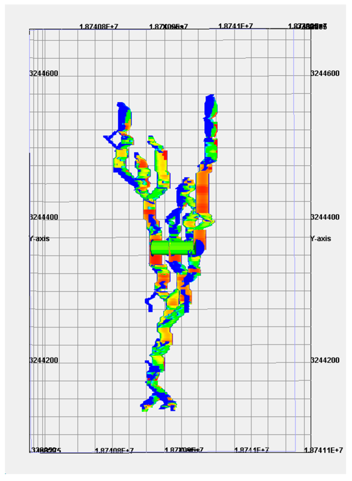
The model was calibrated and accuracy-checked using pre-design microseismic-derived metrics from Well Yi202. The simulated fracture length and effective fracture volume were 394 m and 1258 m³, compared with field-derived calibration targets of 387 m and 1210 m³, giving relative differences of 1.8% and 3.9%, respectively. Because the same well was used to constrain the model, this agreement was treated as calibration/field-based accuracy checking rather than independent validation. The field-derived volume is a microseismic interpretation product rather than a direct volumetric measurement; consequently, comparison with the numerical fracture volume should be interpreted as a model-calibration proxy.

The microseismic catalog was first restricted to events recorded during the hydraulic-fracturing treatment and spatially associated with the target reservoir interval. Events failing the routine location-quality control and isolated events located outside the main stimulated event cluster were excluded. No additional magnitude- or amplitude-based threshold was applied after this quality-control step. A three-dimensional spatial envelope was then constructed from the retained event hypocenters, and the geometric volume enclosed by this event cloud was taken as the microseismic-derived effective fracture volume. This procedure yielded an effective volume of approximately 1210 m³. No additional conversion based on assumed fracture aperture, fracture porosity, proppant concentration, or event magnitude was applied.

2.2. Finite-Element Model Establishment

2.2.1. Geological and Engineering Data

A three-dimensional geomechanical-fracturing model was established (Figure 1) from the geological, logging, and rock-mechanics data of Wells Yi202 and Yi205 (

Table 1. Rock-mechanics and in situ stress parameters of Wells Yi202 and Yi205.

Well	E (GPa)	ν	σH (MPa)	σh (MPa)	Δσh (MPa)	Fracture Pressure (MPa)
Yi202	45.27	0.25	95.40	86.60	8.80	92.40
Yi205	33.30	0.19	94.70	86.10	8.60	95.90
Mean	39.28	0.22	95.05	86.35	8.70	94.15

E, Young’s modulus; ν, Poisson’s ratio; σ_H and σ_h, maximum and minimum horizontal principal stresses; Δσ_h = σ_H − σ_h.

). The computational domain was 500 m × 500 m × 300 m. A nominal Cartesian resolution of 1 m × 1 m × 1 m corresponds geometrically to approximately 75 million continuum cells over the full domain. Hydraulic fractures are represented by displacement-discontinuity surface elements coupled to the geomechanical domain, so the 75-million-cell count describes the host-domain resolution rather than 75 million independent fracture elements.

No formal grid-independence study using additional coarse and fine continuum meshes was performed for the present model, and consequently, mesh-independent convergence was not claimed. The 1 m × 1 m × 1 m discretization was adopted as the base computational resolution for all simulations reported in this study. No adaptive or local refinement of the host-rock continuum grid was applied in the vicinity of propagating fractures. Instead, fracture growth was represented through the displacement-discontinuity fracture elements, whose geometry and connectivity were updated as fracture propagation proceeded. Thus, the evolution of the fracture representation should not be interpreted as adaptive refinement of the underlying continuum mesh. The absence of an explicit coarse/base/fine grid-sensitivity analysis is acknowledged as a limitation of the present study, and future work should quantify the sensitivity of predicted fracture length, fracture volume, and network geometry to continuum-grid resolution.

2.2.2. Boundary Conditions and Loading

The bottom boundary was constrained in the vertical direction, and the lateral boundaries were constrained normal to their respective planes. The maximum and minimum horizontal principal stresses listed in Table 1 were imposed as the far-field horizontal stress state, while a 95 MPa top-boundary traction represented the vertical overburden loading at reservoir depth. The unequal horizontal principal stresses therefore supplied the directional loading asymmetry responsible for stress-induced fracture directionalization.

Self-weight loading was not explicitly included as a gravitational body force in the present model. The effect of the overlying formation was instead represented by imposing a compressive normal traction of 95 MPa on the top boundary, which was taken as the equivalent vertical overburden stress at the modeled reservoir depth. Consequently, gravitational loading was not applied in addition to this boundary traction. This treatment avoids double counting of the overburden contribution to the vertical stress field. Because gravity was not explicitly included, rock density and gravitational acceleration were not introduced as independent loading parameters. The prescribed 95 MPa top traction, together with the imposed in situ stress and displacement boundary conditions, defined the initial mechanical loading state used for the subsequent hydraulic-fracture propagation simulation.

Fracturing fluid was injected at a constant rate, and proppant was introduced according to the prescribed loading per unit lateral length. Each simulation represented 120 min of treatment, consistent with the field operation.

2.3. Symmetry-Breaking Framework and Directionalization Index

Because the intact rock matrix is assumed isotropic, the symmetry considered here is a loading symmetry. Under equal horizontal principal stresses (σ_H = σ_h), the idealized horizontal stress field is directionally invariant. A nonzero horizontal stress difference, Δσ_h = σ_H − σ_h, removes this invariance and selects the maximum-stress direction as the preferred fracture-growth axis. The dimensionless stress-anisotropy coefficient is defined as:

$${\chi }_{\sigma }={\displaystyle \frac{2({\sigma }_H-{\sigma }_h)}{{\sigma }_H+{\sigma }_h}}$$

(9)

where χ_σ = 0 represents equal horizontal stresses and increasing χ_σ represents stronger loading asymmetry. Based on Table 1, χ_σ is 0.0967 for Well Yi202 and 0.0951 for Well Yi205.

To quantify the morphology transition using the available global outputs, a directionalization index I_d is introduced:

$$I_d(\Delta {\sigma }_h)={\displaystyle \frac{L(\Delta {\sigma }_h)/L_0}{V(\Delta {\sigma }_h)/V_0}}={\displaystyle \frac{L(\Delta {\sigma }_h)V_0}{L_{0}V(\Delta {\sigma }_h)}}$$

(10)

where L and V are the simulated average fracture length and fracture volume, respectively, and L₀ and V₀ are the corresponding values for the equal-horizontal-stress reference case (Δσ_h = 0). Because both numerator terms are normalized by quantities with the same units, I_d is dimensionless. For positive L and V, I_d > 0; I_d = 1 denotes the equal-stress reference morphology, I_d > 1 indicates increasing concentration of longitudinal extension relative to volumetric spreading, and I_d < 1 indicates the opposite tendency. Importantly, I_d is a global directionalization proxy rather than a geometrical reflection-symmetry metric: it can increase because L grows, V contracts, or both. It therefore does not by itself identify the mechanism responsible for a change in fracture geometry.

2.4. Sensitivity Analysis and Engineering Design Selection

A one-factor-at-a-time (OFAT) sensitivity design was used to quantify the main effects of geomechanical and engineering variables (

Table 2. Sensitivity scheme for geomechanical parameters.

Parameter	Tested Values	Fixed Parameters
Young’s modulus (GPa)	26, 30, 34, 38, 42	Poisson’s ratio = 0.22; horizontal stress difference = 8.7 MPa
Poisson’s ratio	0.10, 0.15, 0.20, 0.25, 0.30	Young’s modulus = 39.28 GPa; horizontal stress difference = 8.7 MPa
Horizontal stress difference (MPa)	0, 3, 6, 9, 12, 15	Young’s modulus = 39.28 GPa; Poisson’s ratio = 0.22

and

Table 3. Sensitivity scheme for engineering parameters.

Well	Parameter	Tested Values	Fixed Parameters
Yi202	Injection rate (m3/min)	6, 10, 14, 18, 22	Fluid-volume intensity = 37.5 m3/m; proppant loading = 1.3 t/m
Yi202	Fluid-volume intensity (m3/m)	16.67, 25, 33.34, 41.67, 50.00, 58.33	Injection rate = 10.7 m3/min; proppant loading = 1.3 t/m
Yi202	Proppant loading (t/m)	0.1, 0.5, 1.0, 2.0, 3.0, 4.0	Injection rate = 10.7 m3/min; fluid-volume intensity = 37.5 m3/m
Yi205	Injection rate (m3/min)	6, 10, 14, 18, 22	Fluid-volume intensity = 32.5 m3/m; proppant loading = 3.2 t/m
Yi205	Fluid-volume intensity (m3/m)	16.67, 25, 33.34, 41.67, 50.00, 58.33	Injection rate = 16.6 m3/min; proppant loading = 3.2 t/m
Yi205	Proppant loading (t/m)	0.1, 0.5, 1.0, 2.0, 3.0, 4.0	Injection rate = 16.6 m3/min; fluid-volume intensity = 32.5 m3/m

). The OFAT results are used for parameter screening and physics-guided engineering design selection; they do not resolve interaction terms and therefore do not establish a joint or global mathematical optimum. Final well-specific parameter combinations were evaluated as combined design cases in the engineering assessment. Some implemented values were field-oriented selections between or within the discrete screening levels (for example, q = 16 m³/min for Yi205 and Vf = 45.8 m³/m for Yi202), and were therefore distinguished from the discrete OFAT simulation points. The original simulation-output plots retain the export labels “displacement”, “liquid volume intensity”, and “proppant concentration”; these correspond to injection rate, fluid-volume intensity, and proppant loading, respectively.

2.5. Production-Forecast and EUR Evaluation

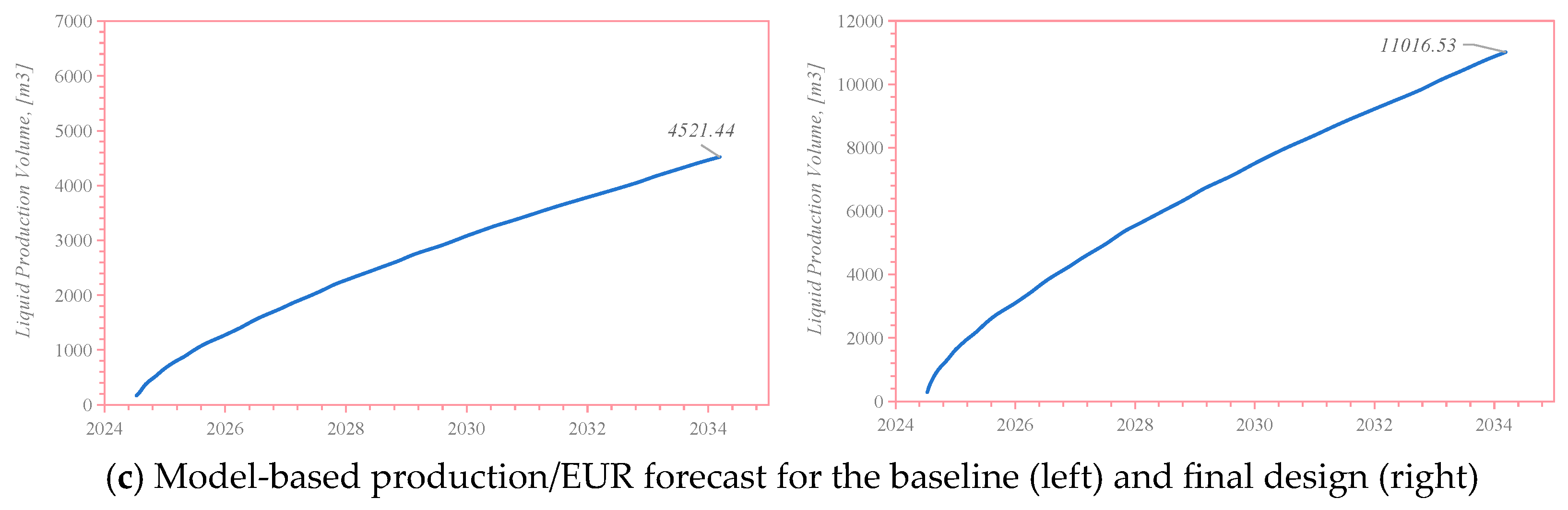
The production profiles represent model-based forecasts over the period 2024–2034 and therefore correspond to a 10-year forecast horizon rather than to observed 10-year production. The reported estimated ultimate recovery (EUR) values were derived from these forecast production profiles and were used as comparative engineering indicators to evaluate the relative production performance of the baseline and optimized fracture designs.

The production-forecast analysis was conducted independently from the microseismic calibration and fracture-volume comparison. Accordingly, the microseismic-derived fracture characteristics were used primarily to constrain and assess the fracture geometry, whereas the production forecasts were used to evaluate the expected long-term production response associated with different stimulation designs. The EUR values should therefore not be interpreted as direct measurements derived from microseismic data or simulated fracture volume.

The archived study records available for the present revision do not contain sufficient information to reconstruct the exact production-forecast implementation, including the specific forecasting software/version, production-history interval used for calibration, detailed decline or reservoir-flow assumptions, operational forecast constraints, economic/abandonment criteria, or formal uncertainty range. These parameters are therefore not inferred or retrospectively assigned in the revised manuscript. Consequently, the reported EUR values are interpreted as deterministic model-based comparative forecasts under the original study assumptions, rather than as independently reproducible reserve estimates. The absence of documented forecast-sensitivity or uncertainty analysis is acknowledged as a limitation of the present study.

3. Results

3.1. Geomechanical Controls on Fracture Symmetry and Directionality

3.1.1. Young’s Modulus

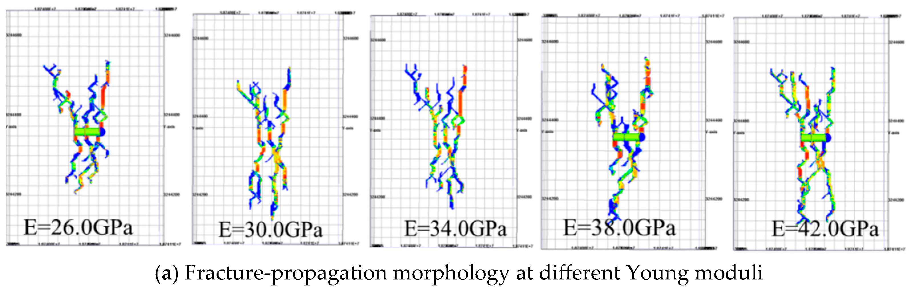
As Young’s modulus increased from 26 to 42 GPa, fracture volume increased from 1258 to 1695 m³, corresponding to a 35% increase (Figure 2). The simulated morphologies also showed more developed branching at a higher modulus. Within the adopted elastic framework, a larger Young’s modulus is associated with a more brittle response and a greater tendency for injected energy to generate and extend fracture branches. The coefficient of determination between Young’s modulus and fracture volume was R² = 0.96, indicating a strong positive relationship over the tested range.

3.1.2. Poisson’s Ratio

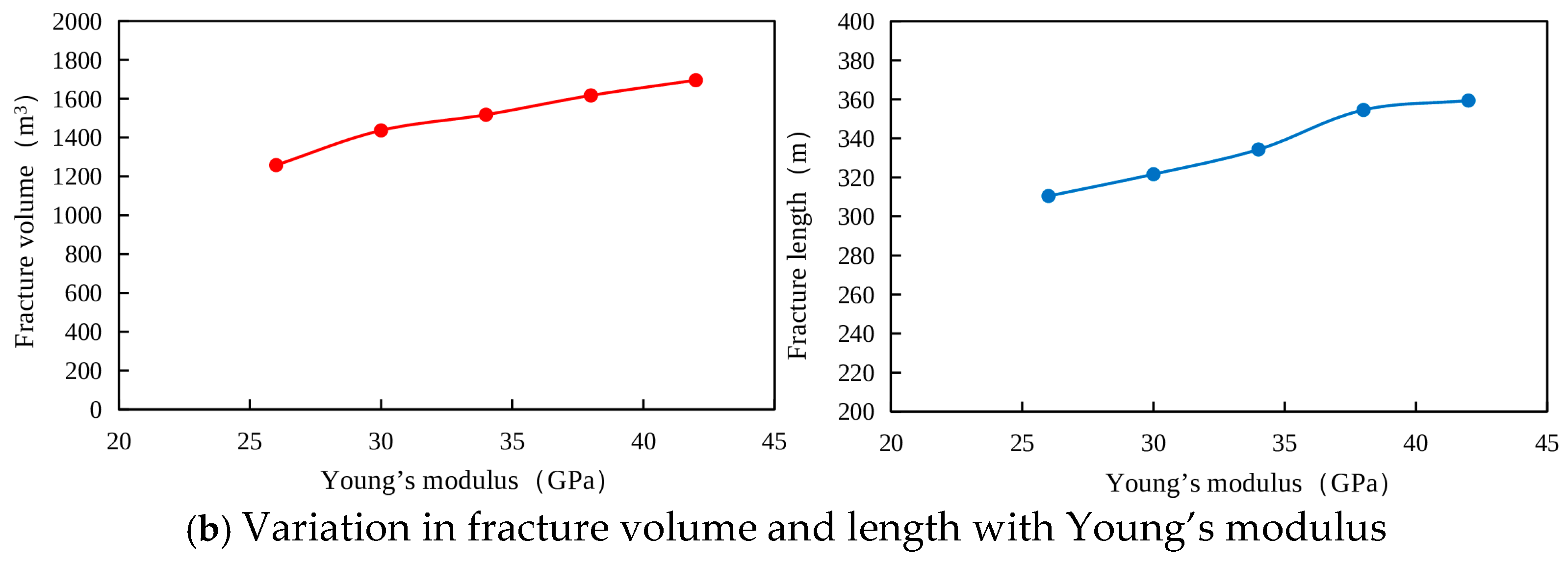
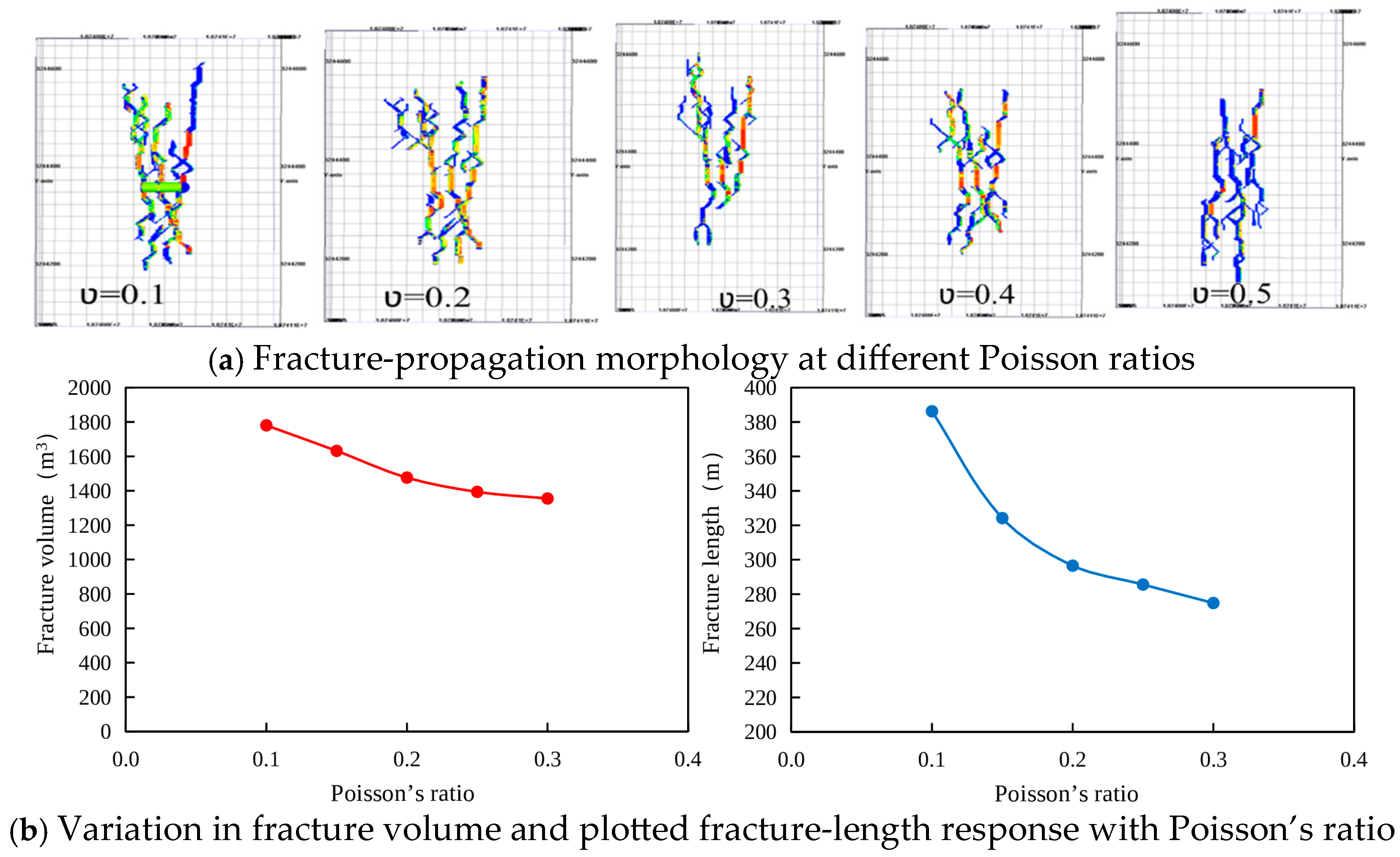
When Poisson’s ratio increased from 0.10 to 0.30, fracture volume decreased by approximately 24%, and the plotted average fracture length decreased from approximately 386 to 275 m (Figure 3). The previously reported millimeter unit was a transcription error; the fracture-length axis and all corresponding results were in meters. Larger Poisson’s ratio increases lateral deformation coupling and, in the present model, reduces the opening and branching response under the same injection conditions. The relationship between Poisson’s ratio and fracture volume remained strongly negative over the tested range.

3.1.3. Horizontal-Stress-Difference-Induced Symmetry Breaking

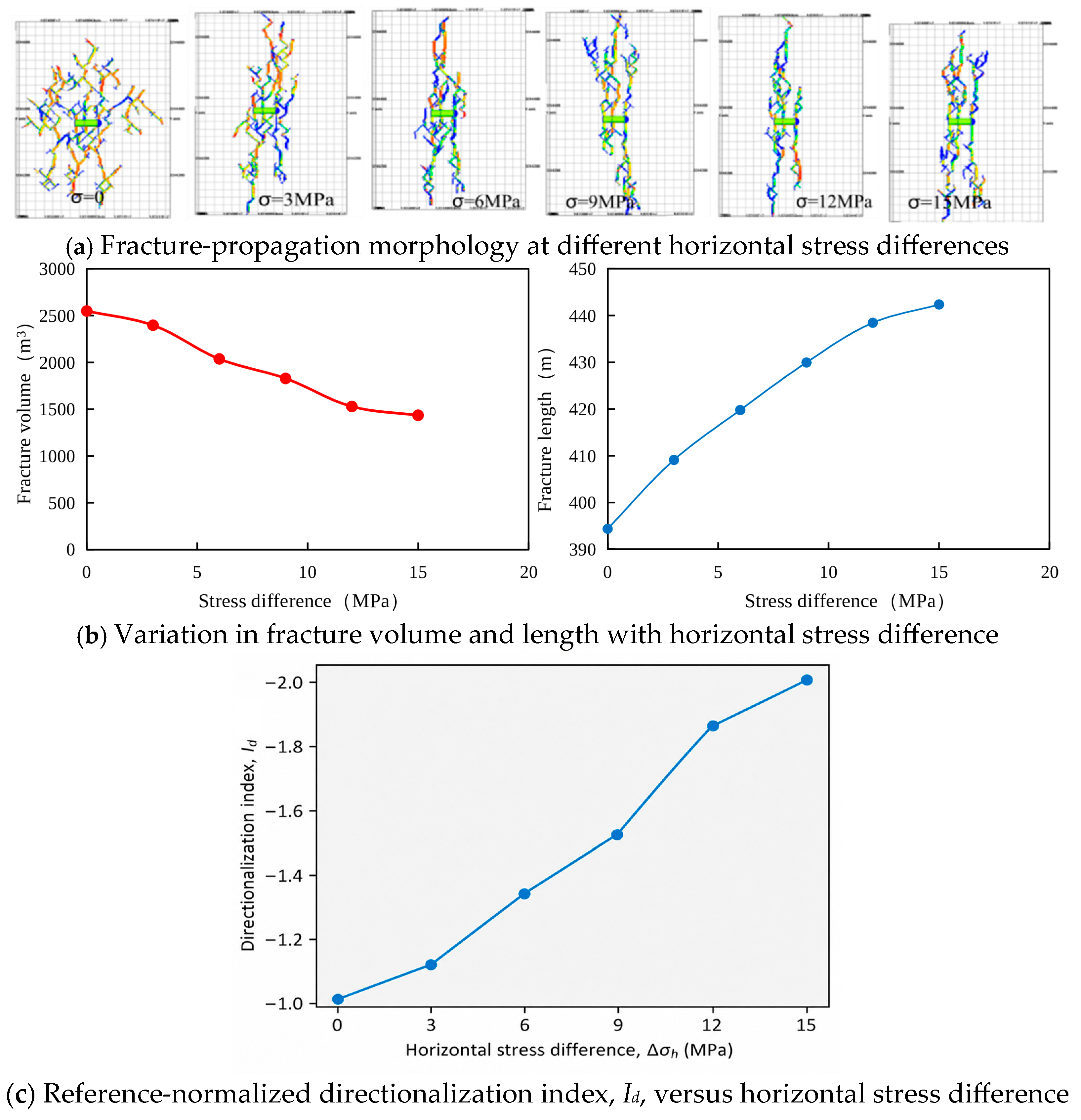
Increasing the horizontal stress difference from the equal-stress reference (Δσ_h = 0) to 15 MPa reduced fracture volume from 2549 to 1435 m³ (approximately 44%), while average fracture length increased from 394 to 442 m (approximately 12%) (Figure 4). The morphology therefore changed from a comparatively distributed and branched pattern to a more elongated pattern aligned with the maximum horizontal principal stress. Using Equation (10), I_d increased from 1.00 at 0 MPa to 1.99 at 15 MPa. At 15 MPa, L/L₀ = 1.122, whereas V/V₀ = 0.563; therefore, the increase in I_d was driven predominantly by contraction of volumetric spreading rather than by length growth alone. A logarithmic decomposition, ln(I_d) = ln(L/L₀) − ln(V/V₀), attributes approximately 17% of the change in ln(I_d) to length growth and 83% to reduced volume retention. Accordingly, I_d is interpreted as a directional concentration proxy, not as a measure of “extension enhancement” alone.

The geomechanical variables analyzed in Section 3.1 are reservoir constraints rather than controllable design variables. Their role is therefore to define the response regime within which engineering parameters are selected. In particular, larger horizontal stress contrast promotes directional concentration and reduces volumetric spreading, whereas less favorable elastic properties reduce fracture opening/branching. Section 3.2 consequently evaluates controllable injection rate, fluid-volume intensity, and proppant loading as compensating engineering controls for each well’s measured geomechanical state. This transition is a physics-guided design-selection step, not an attempt to “optimize” the geological parameters themselves.

3.2. Well-Specific Engineering-Parameter Screening and Design Selection

3.2.1. Injection Rate

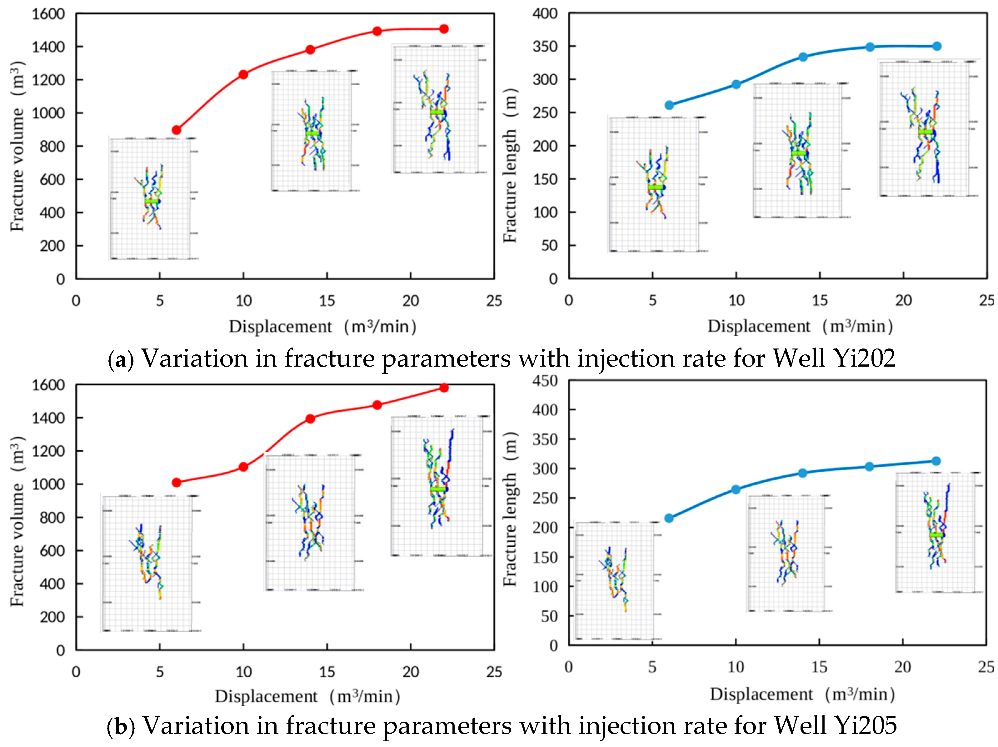
For Well Yi202, the OFAT response increased rapidly between 6 and 18 m³/min and then approached a plateau between 18 and 22 m³/min (Figure 5a); 18 m³/min was therefore retained as the field design value. For Well Yi205, the screening curve continued to increase over the tested 6–22 m³/min range (Figure 5b). The implemented value of 16 m³/min in

Table 4. Well-specific field design values and model-based combined-case engineering evaluation.

Well	q (m3/min)	Vf (m3/m)	Mp (t/m)	Simulated Fracture Volume (m3)	Volume Increase (%)	EUR Forecast (108 m3)	EUR Increase (%)
Yi202	18	45.8	2.0	1600	27	0.63	40
Yi205	16	33.34	3.0	1558	18	0.58	36

q, injection rate; V_f, fluid-volume intensity; M_p, proppant loading; EUR, estimated ultimate recovery. Fracture-volume values are combined-case numerical outputs; EUR values are model-based forecasts rather than direct field measurements.

lies between the 14 and 18 m³/min screening cases and is treated as a field-oriented design selection rather than as the simulated global maximum. The two wells therefore support a practical design window of approximately 14–18 m³/min while also illustrating why the selected value should remain well-specific.

3.2.2. Fluid-Volume Intensity

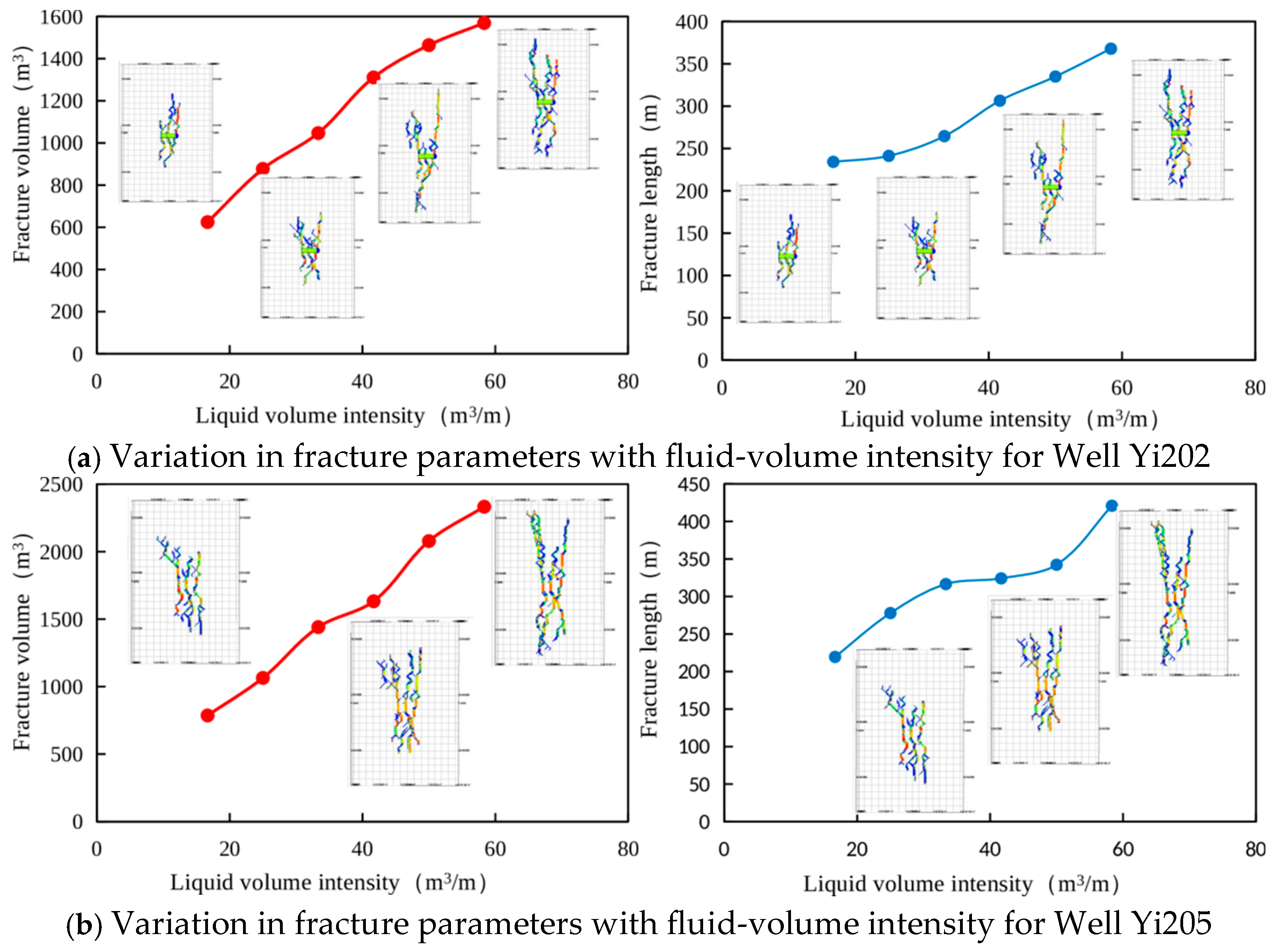
The discrete OFAT screening curves for fluid-volume intensity increased across the tested 16.67–58.33 m³/m range for both wells (Figure 6). Accordingly, the implemented values in Table 4 are not described as simulated maxima. For Yi202, the field-tuned value of 45.8 m³/m lies between the 41.67 and 50.00 m³/m screening levels and is retained as an engineering design value within the rising-response regime. For Yi205, 33.34 m³/m is one of the discrete screening levels and is retained as the well-specific field design value despite the continued numerical increase at higher fluid-volume intensity. These choices distinguish field-oriented design selection from a mathematical optimum and avoid implying a universal block-wide value.

3.2.3. Proppant Loading

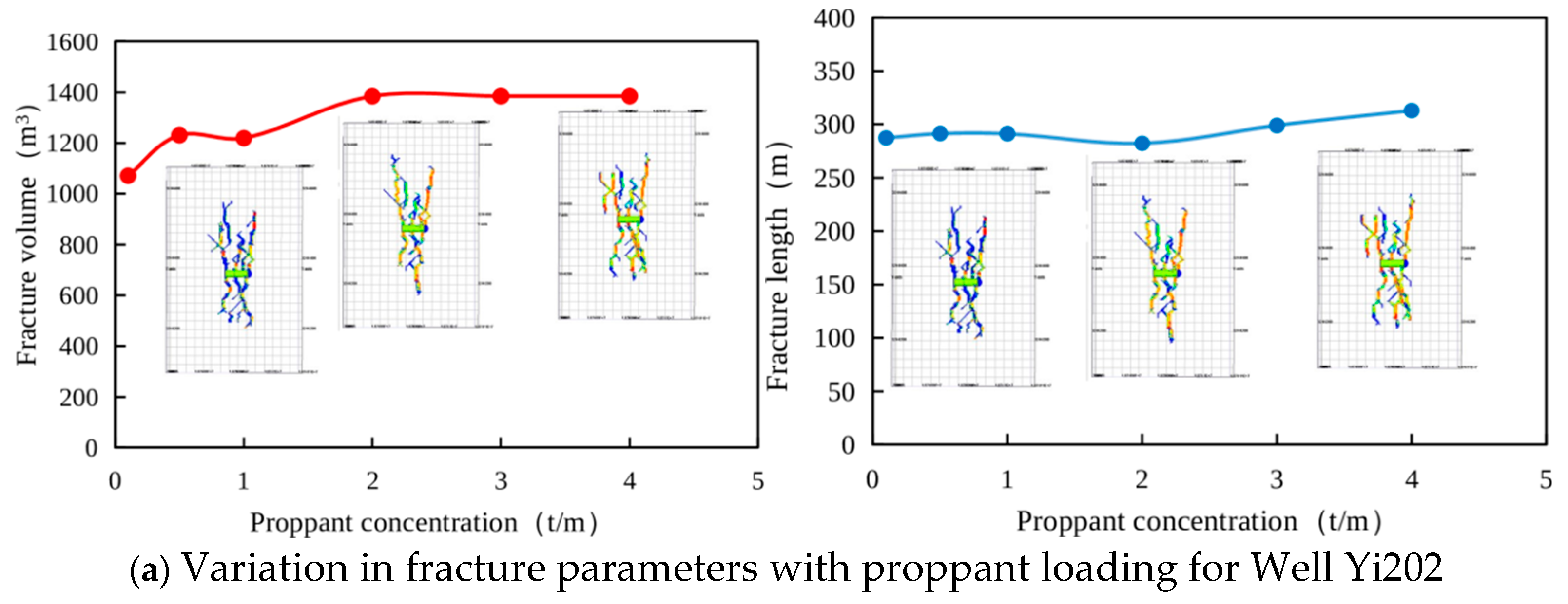
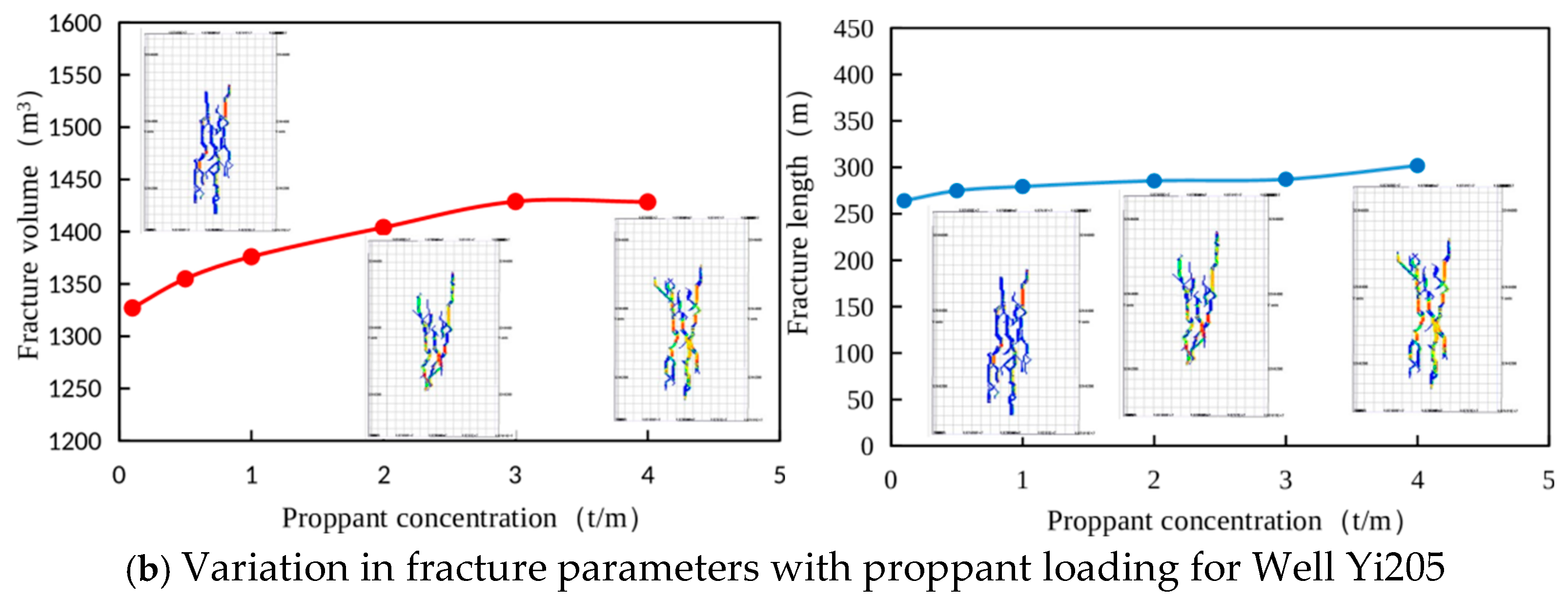
For Well Yi202, the proppant-loading response increased up to approximately 2 t/m and then changed only slightly, whereas Well Yi205 showed its largest plotted fracture volume near 3 t/m (Figure 7). The selected field design values were therefore 2.0 t/m for Yi202 and 3.0 t/m for Yi205. These values were treated as engineering selections from the OFAT screening response, not as proof of a joint multi-variable optimum.

3.3. Field Application and Production Response

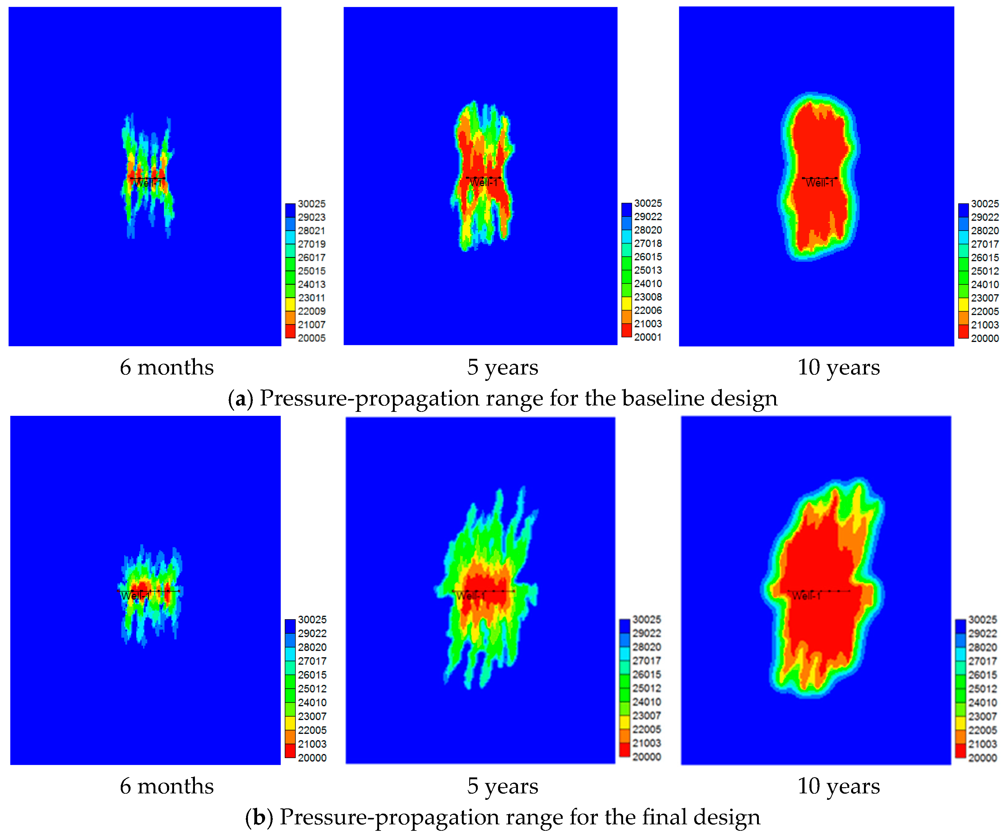
The final well-specific parameter combinations were evaluated as combined design cases and were subsequently used in the field-oriented engineering assessment (Table 4). The fracture-volume values reported in Table 4 are numerical outputs from the combined design cases, whereas the EUR values are model-based production forecasts; neither quantity should be interpreted as a direct field measurement of future fracture volume or 10-year recovery. For Yi202, simulated fracture volume increased from the calibrated baseline of 1258 to 1600 m³ (27%), and the EUR forecast increased from 0.45 × 10⁸ to 0.63 × 10⁸ m³ (40%). For Yi205, the combined-case simulated fracture volume increased from 1320 to 1558 m³ (18%), and the reported final EUR forecast was 0.58 × 10⁸ m³, corresponding to a 36% increase relative to its baseline forecast. These results are therefore presented as comparative engineering-evaluation outputs rather than independent field validations (Figure 8).

4. Discussion

4.1. Physical Interpretation of Stress-Induced Symmetry Breaking

The model separates two conceptually different sources of fracture behavior. Young’s modulus and Poisson’s ratio control the elastic response and the tendency to generate fracture opening and branching, whereas unequal horizontal principal stresses break the directional invariance of the loading field. Because the constitutive matrix is assumed to be isotropic, the preferred propagation direction is not attributed to intrinsic material anisotropy. Instead, it is boundary-condition-induced symmetry breaking in which σH defines a preferred axis and increasing Δσ_h progressively suppresses transverse volumetric spreading. The reference-normalized Id metric tracks this directional concentration but should not be interpreted as a direct geometrical symmetry index.

Engineering parameters regulate how strongly stimulation responds to this broken-symmetry stress environment. Injection rate controls pressure build-up and activation of additional fracture elements, fluid-volume intensity controls the spatial reach of pressure communication and fracture extension, and proppant loading controls post-opening support and conductivity. These controllable variables cannot restore geological symmetry; instead, they are selected to compensate for well-specific stress and elastic constraints. Consistent with productivity studies that couple fracture-network evolution to well performance, the combined-design evaluation links the fracture response to a forecasted engineering outcome without claiming a joint mathematical optimum.

Natural fractures and bedding can modify the symmetry-breaking response in ways that are not represented explicitly here. Preferentially oriented natural-fracture sets may reinforce stress-selected propagation if they are favorably aligned with σH, whereas oblique or transverse discontinuities can provide competing pathways, locally increase branching, or partly counter the volumetric suppression caused by stress contrast [8,16]. The present isotropic model should therefore be read as isolating the first-order loading-induced component of directionalization. Its branch geometry arises from hydraulic-fracture-element interactions and stress-shadow effects, not from activation of a mapped natural-fracture network; consequently, absolute branch density and local asymmetry may differ from field behavior even when the stress-controlled directional trend is captured.

4.2. Relation to Previous Studies and Engineering Implications

The positive effect of Young’s modulus and the negative effect of Poisson’s ratio on fracture development are consistent with conventional fracability concepts [9] and with the unequal elastic-parameter weighting reported by Suo et al. [25]. The stress-difference response agrees with studies showing that larger stress contrast promotes fracture alignment and suppresses network complexity [16]. Compared with the symmetry-enhanced hydraulic-fracturing simulation of Wang et al. [24], the present work emphasizes the loss of loading symmetry and explicitly normalizes directionalization to the equal-stress case. The microseismic-based morphology analysis of Lin et al. [26] supports the use of field observations to constrain fracture geometry. The added value of the present framework is therefore the separation of loading symmetry from material isotropy, the quantitative L–V directionalization proxy, and the subsequent use of geomechanical response regimes to guide well-specific engineering design selection rather than a universal “optimal” treatment.

4.3. Limitations and Future Work

This study has several limitations. First, natural fractures and bedding heterogeneity are not represented explicitly, so the model isolates loading-induced directionalization but cannot reproduce all sources of field-scale asymmetry or branch activation. Second, calibration and accuracy checking rely mainly on one pre-design well; independent validation with additional microseismic datasets is still required. Third, Id is a global proxy derived from fracture length and volume, not a direct reflection-symmetry metric calculated from event coordinates; future work should quantify orientation distributions, left–right area imbalance, branch density, centroid offset, and fracture-orientation entropy using raw monitoring data. Fourth, the OFAT design does not quantify interaction terms among stress, injection rate, fluid volume, and proppant loading; factorial, response-surface, or Bayesian design studies are needed to establish a true multi-variable optimum. Fifth, a complete mesh-convergence dataset is not available in the present study, so grid-independence is not demonstrated quantitatively and should be evaluated in future numerical work. Sixth, the microseismic volume conversion and EUR forecasting workflow require explicit reporting of their processing assumptions and uncertainty. Finally, long-term proppant embedment and conductivity degradation are not included. These limitations do not alter the observed first-order stress-controlled trend, but they bound the transferability and quantitative precision of the present engineering evaluation.

5. Conclusions

• Horizontal stress difference acts as an external loading-symmetry-breaking control in the idealized isotropic model. The physically symmetric reference is Δσ_h = 0, and the field stress-anisotropy coefficients χ_σ = 0.0967 for Yi202 and 0.0951 for Yi205 indicate comparable directional loading in the two wells.
• Increasing Δσ_h from 0 to 15 MPa reduced fracture volume by approximately 44% and increased average fracture length by approximately 12%. The reference-normalized directionalization proxy Id increased from 1.00 to 1.99. This increase was dominated by reduced volume retention rather than length growth alone, so Id was interpreted as a measure of directional concentration rather than pure extension enhancement.
• The engineering design selection was well-dependent. The final combined design used 18 m³/min, 45.8 m³/m, and 2.0 t/m for Yi202 and 16 m³/min, 33.34 m³/m, and 3.0 t/m for Yi205. These parameter sets were field-oriented combined designs informed by OFAT screening, not mathematically proven global optima.
• The final combined design cases increased simulated fracture volume by 18–27%, while the model-based EUR forecasts increased by 36–40%. These results support the engineering value of adapting treatment design to the local geomechanical response regime, while the distinction among simulation outputs, microseismic calibration metrics, and production forecasts should be maintained.

References

1. Zou, C.; Dong, D.; Wang, S.; Li, J.; Li, X.; Wang, Y.; Li, D.; Cheng, K. Geological characteristics and resource potential of shale gas in China. Pet. Explor. Dev. 2015, 37, 641–653. [Google Scholar] [CrossRef] [Scilit]
2. Zhai, G.Y.; Wang, Y.F.; Zhou, Z.; Yu, S.F.; Chen, X.L.; Zhang, Y.X. Exploration and research progress of shale gas in China. China Geol. 2018, 1, 257–272. [Google Scholar] [CrossRef] [Scilit]
3. Shi, X.; Kang, S.; Luo, C.; Wu, W.; Zhao, S.; Zhu, D.; Zhang, H.; Yang, Y.; Xiao, Z.; Li, Y. Shale gas exploration potential and reservoir conditions of the Longmaxi Formation in the Changning area, Sichuan Basin, SW China: Evidence from mud gas isotope logging. J. Asian Earth Sci. 2022, 233, 105239. [Google Scholar] [CrossRef] [Scilit]
4. Jin, X.; Shah, S.N.; Roegiers, J.C.; Zhang, B. Fracability Evaluation in Shale Reservoirs—An Integrated Petrophysics and Geomechanics Approach. In Proceedings of the SPE Hydraulic Fracturing Technology Conference, The Woodlands, TX, USA, 4–6 February 2014. [Google Scholar] [CrossRef] [Scilit]
5. Li, Q.; Li, Q.; Wang, F.; Xu, N.; Wang, Y.; Bai, B. Settling behavior and mechanism analysis of kaolinite as a fracture proppant of hydrocarbon reservoirs in CO2 fracturing fluid. Colloids Surf. A Physicochem. Eng. Asp. 2025, 724, 137463. [Google Scholar] [CrossRef] [Scilit]
6. Li, Q.; You, D.; Li, Q.; Wang, F.; Wang, Y.; Yang, Y. Analysis of Sedimentation Behavior and Influencing Factors of Solid Particles in CO2 Fracturing Fluid. Processes 2025, 13, 4049. [Google Scholar] [CrossRef] [Scilit]
7. Meyer, B.R.; Bazan, L.W. A discrete fracture network model for hydraulically induced fractures—Theory, parametric, and case studies. In Proceedings of the SPE Hydraulic Fracturing Technology Conference, The Woodlands, TX, USA, 24–26 January 2011. [Google Scholar] [CrossRef] [Scilit]
8. Nelson, R.A. Geologic Analysis of Naturally Fractured Reservoirs; Elsevier: Amsterdam, The Netherlands, 2001. [Google Scholar] [CrossRef] [Scilit]
9. Veatch, R.W. Overview of Current Hydraulic Fracturing Design and Treatment Technology—Part 2. J. Pet. Technol. 1983, 35, 853–864. [Google Scholar] [CrossRef] [Scilit]
10. Ozkan, E.; Raghavan, R.; Apaydin, O.G. Modeling of fluid transfer from shale matrix to fracture network. In Proceedings of the SPE Annual Technical Conference and Exhibition, Florence, Italy, 19–22 September 2010. [Google Scholar] [CrossRef] [Scilit]
11. Wu, Y.; Cheng, L.; Huang, S.; Xue, Y.; Ding, G. A semi-analytical method of production prediction for shale gas wells considering multi-nonlinearity of flow mechanisms. Sci. Sin. Technol. 2018, 48, 691–700. [Google Scholar] [CrossRef] [Scilit]
12. Liu, J.; Xie, L.Z.; He, B.; Zhao, P.; Ding, H.-Y. Performance of free gases during the recovery enhancement of shale gas by CO2 injection: A case study on the depleted Wufeng–Longmaxi shale in northeastern Sichuan Basin, China. Pet. Sci. 2021, 18, 530–545. [Google Scholar] [CrossRef] [Scilit]
13. Xu, W.; Le Calvez, J.H.; Thiercelin, M.J. Characterization of a hydraulically induced fracture network using treatment and microseismic data in a tight-gas sand formation: A geomechanical approach. In Proceedings of the SPE Tight Gas Completions Conference, Denver, CO, USA, 15–17 June 2009. [Google Scholar] [CrossRef] [Scilit]
14. Li, Y.; Deng, J.; Liu, W.; Yan, W.; Feng, Y.; Cao, W.; Wang, P.; Hou, Y. Numerical simulation of limited-entry multi-cluster fracturing in horizontal well. J. Pet. Sci. Eng. 2017, 152, 443–455. [Google Scholar] [CrossRef] [Scilit]
15. Li, W.; Zhang, T.; Liu, X.; Dong, Z.; Dong, G.; Qian, S.; Yang, Z.; Zou, L.; Lin, K.; Zhang, T. Machine learning-based fracturing parameter optimization for horizontal wells in Panke field shale oil. Sci. Rep. 2024, 14, 6046. [Google Scholar] [CrossRef] [Scilit] [PubMed]
16. Ren, L.; Lin, R.; Zhao, J.; Wu, L. An optimal design of cluster-spacing intervals for staged fracturing in horizontal shale gas wells based on the optimal SRVs. Nat. Gas Ind. B 2017, 4, 364–373. [Google Scholar] [CrossRef] [Scilit]
17. Lin, R.; Ren, L.; Zhao, J. Cluster-spacing optimization for horizontal-well fracturing in shale gas reservoirs: Modeling and field application. In Proceedings of the SPE Europec Featured at the 80th EAGE Conference and Exhibition, Copenhagen, Denmark, 14–18 June 2018. [Google Scholar] [CrossRef] [Scilit]
18. Zhao, J.; Tang, H.; Xue, S. A new fracture criterion for peridynamic and dual-horizon peridynamics. Front. Struct. Civ. Eng. 2017, 12, 629–641. [Google Scholar] [CrossRef] [Scilit]
19. Gordeliy, E.; Peirce, A. Coupling schemes for modeling hydraulic fracture propagation using the XFEM. Comput. Methods Appl. Mech. Eng. 2013, 253, 305–322. [Google Scholar] [CrossRef] [Scilit]
20. Esfandiari, M.; Pak, A. XFEM modeling of the effect of in-situ stresses on hydraulic fracture characteristics and comparison with KGD and PKN models. J. Pet. Explor. Prod. Technol. 2023, 13, 185–201. [Google Scholar] [CrossRef] [Scilit]
21. Liu, J.; Wang, J.; Leung, C.; Gao, F. A Multi-Parameter Optimization Model for the Evaluation of Shale Gas Recovery Enhancement. Energies 2018, 11, 654. [Google Scholar] [CrossRef] [Scilit]
22. Li, Q.; Li, Y.; Cheng, Y.; Li, Q.; Wang, F.; Wei, J.; Liu, Y.; Zhang, C.; Song, B.; Yan, C.; et al. Numerical simulation of fracture reorientation during hydraulic fracturing in perforated horizontal well in shale reservoirs. Energy Sources Part A Recovery Util. Environ. Eff. 2018, 40, 1807–1813. [Google Scholar] [CrossRef] [Scilit]
23. Chen, P.; Jiang, S.; Chen, Y.; Zhang, K. Pressure response and production performance of volumetric fracturing horizontal well in shale gas reservoir based on boundary element method. Eng. Anal. Bound. Elem. 2018, 87, 66–77. [Google Scholar] [CrossRef] [Scilit]
24. Wang, C.; Yue, Y.; Huang, Z.; Tong, Y.; Zhang, W.; Ye, S. A new symmetry-enhanced simulation approach considering poromechanical effects and its application in the hydraulic fracturing of a carbonate reservoir. Symmetry 2024, 16, 105. [Google Scholar] [CrossRef] [Scilit]
25. Suo, Y.; Li, F.; Liang, Q.; Huang, L.; Yi, L.; Dong, X. Weight-based numerical study of shale brittleness evaluation. Symmetry 2025, 17, 927. [Google Scholar] [CrossRef] [Scilit]
26. Lin, L.; Xiong, X.; Xu, Z.; Yan, X.; Wang, Y. Characterizing hydraulic-fracture morphology and propagation patterns in horizontal-well stimulation via micro-seismic monitoring analysis. Symmetry 2025, 17, 1732. [Google Scholar] [CrossRef] [Scilit]
Figure 1. Field-calibrated fracture-propagation model.
Symmetry 18 01495 g001
Figure 2. Effect of Young’s modulus on fracture-network evolution.
Symmetry 18 01495 g002aSymmetry 18 01495 g002b
Figure 3. Effect of Poisson’s ratio on fracture-network evolution.
Symmetry 18 01495 g003
Figure 4. Effect of horizontal stress difference on fracture-network directionalization: (a) fracture-propagation morphology; (b) fracture volume and length; and (c) reference-normalized directionalization index. The Δσh = 0 case is the equal-horizontal-stress reference state.
Symmetry 18 01495 g004
Figure 5. Effect of injection rate on fracture propagation for Wells Yi202 and Yi205. The simulator-export x-axis label “Displacement” corresponds to injection rate (m3/min).
Symmetry 18 01495 g005
Figure 6. Effect of fluid-volume intensity on fracture propagation for Wells Yi202 and Yi205. The discrete screening levels were 16.67, 25.00, 33.34, 41.67, 50.00, and 58.33 m3/m.
Symmetry 18 01495 g006
Figure 7. Effect of proppant loading on fracture propagation for Wells Yi202 and Yi205. The simulator-export label “proppant concentration” corresponds to proppant loading (t/m).
Symmetry 18 01495 g007aSymmetry 18 01495 g007b
Figure 8. Pressure-propagation and model-based production/EUR forecast for the baseline and final combined design of Well Yi202; the forecast horizon shown is 2024–2034.
Symmetry 18 01495 g008aSymmetry 18 01495 g008b