Multi-Objective Optimization of a High-Temperature Flange–Bolt–Gasket System Based on a Cyclic Symmetric Thermal–Structural Coupling Model

Abstract

The high-temperature sealing reliability of flange–bolt–gasket systems is governed by the coupled gasket leakage, flange cracking, and bolt yielding. This study investigates a DN200 PN40 (nominal diameter 200 mm and nominal pressure 4.0 MPa) weld-neck flange assembly operating under 300 °C superheated steam at 4 MPa internal pressure. Exploiting the assembly’s 12-fold cyclic rotational symmetry, a 1/12 periodic-sector finite element model with steady-state thermal–structural sequential coupling was developed in ANSYS Workbench and validated against the Omiya–Sawa 3-inch weld-neck flange benchmark at two levels (Level 1: bolt load vs. experiment; Level 2: 250 °C gasket contact pressure vs. reference finite element method (FEM)), with maximum errors below 1.5% in both levels; the benchmark thus establishes the reliability of the modeling procedure rather than constituting a direct experimental validation of the DN200 PN40 configuration. Using a central composite design, second-order response surface models (RSM) and Kriging surrogate models were constructed and compared, followed by Sobol global sensitivity analysis, multi-objective optimization using the non-dominated sorting genetic algorithm II (NSGA-II), and decision-making using the technique for order preference by similarity to ideal solution (TOPSIS), with bolt preload F and gasket width b as design variables. Baseline analysis revealed a differential contact pressure distribution—lower at the inner radius and higher at the outer radius—driven by a −0.308° flange rotation, identifying the inner gasket edge as the critical sealing failure path. RSM outperformed Kriging for the primary objective (mean absolute percentage error (MAPE): 0.72% vs. 3.61%), and the Pareto front collapsed to b = 19 mm. The TOPSIS-recommended optimum (F = 59,942 N, b = 19.00 mm), verified by ANSYS back-substitution, increased the minimum gasket contact pressure by 31.01% while reducing the flange membrane-plus-bending stress by 2.26%, achieving a coordinated improvement of both sealing performance and structural safety.

1. Introduction

The bolted flange–gasket connection is the most widely used detachable sealing assembly between pressure vessels and piping systems, and finds broad application in critical industries including petrochemical processing, nuclear power generation, electric power, and long-distance natural gas transmission [1]. Compared with welded joints, flanged connections offer notable advantages in ease of installation, repeated disassembly, and maintenance accessibility; however, their sealing reliability has long been a concern for both engineering practitioners and researchers. According to the European Major Accident Reporting System (eMARS), approximately 6% of the 727 major chemical accidents recorded since 2000 were directly attributable to bolted flange failures, corresponding to an average of two major incidents per year, accompanied by approximately 4.1 injuries and 0.65 fatalities annually [2]. Flange leakage is also one of the two primary sources of fugitive emissions in refining and petrochemical operations, posing an ongoing challenge to regulatory compliance and process safety. Improving the sealing reliability of bolted flange–gasket systems under demanding operating conditions therefore remains a central research priority in engineering practice.

Among the various service conditions encountered in practice, sealing under high-temperature steam (including both saturated and superheated regimes) and elevated pressure-temperature media is particularly challenging. On one hand, elevated temperatures substantially alter the elastic modulus, thermal expansion coefficient, and allowable stress of flange and bolt materials, causing progressive bolt preload relaxation over service time [3]. On the other hand, differential thermal expansion among the flange body, bolts, and gasket—driven by material mismatch in thermal expansion coefficients and temperature gradients—redistributes gasket contact stress, creating localized under-compression at the sealing interface and inducing leakage [4,5]. Marek et al. [3] demonstrated that thermal cyclic loading significantly accelerates bolt preload relaxation. Jaszak et al. [4,6] systematically examined the influence of sealing surface microstructure on leakage rate through combined computational fluid dynamics (CFD) simulation and experimentation. Grzejda et al. [5] revealed the coupled effects of design parameters—including winding strip inclination angle and fill density—on the axial stiffness of spiral wound gaskets. Taken together, these studies indicate that the sealing performance of bolted flange–gasket systems under high-temperature conditions is governed by nonlinear coupling among material properties, geometry, temperature distribution, and load history, and cannot be accurately captured by classical linear-elastic analytical methods such as the American Society of Mechanical Engineers (ASME) m–y procedure.

Early investigations into flange sealing behavior predominantly relied on Waters’ flange rotation theory and the ASME m–y method, whose axisymmetric elastic assumptions are inadequate to represent three-dimensional nonlinear deformation. Sawa et al. [7] conducted systematic elastoplastic finite element analyses and spiral wound gasket leakage experiments across pipe flanges ranging from 2″ to 20″ nominal diameter, revealing the critical role of flange rotation in governing contact stress distribution. Concurrently, Takagi, Omiya, and colleagues [8] performed simulation and experimental investigations of a 3″ spiral wound gasket flange subjected to cyclic thermal loading, finding that thermal expansion mismatch markedly alters the contact stress distribution. Fukuoka and Nomura [9] subsequently incorporated the high-temperature compressive behavior of gaskets into finite element models. Bouzid and Nechache [10,11] developed creep-relaxation prediction models suitable for engineering design. Abid [12] used three-dimensional nonlinear finite element analysis to establish safe operating boundaries under combined internal pressure and steady-state thermal loading. More recently, Bian et al. [13] proposed a time-varying leakage rate prediction method based on equivalent stress–temperature relationships. These works collectively establish the analytical foundation for studying sealing behavior in high-temperature bolted flange–gasket systems.

With advances in commercial finite element software, three-dimensional nonlinear thermal–structural coupled analysis has become the prevailing tool for investigating the sealing behavior of bolted flange–gasket assemblies [14]. Murali Krishna et al. [15,16] employed an anisotropic Hill plasticity constitutive model to quantify the radial non-uniformity of contact stress induced by flange rotation. Wang et al. [17] and Yun et al. [18] investigated transient and steady-state thermal–structural coupled sealing problems in subsea connectors, respectively, finding that non-uniform temperature distributions substantially amplify stress redistribution at the sealing interface. However, these studies largely focus on qualitative mechanistic analysis under single operating conditions. For parametric optimization problems involving multiple variables and competing objectives, the conventional approach of parameter sweeping with point-by-point simulation is computationally inefficient and ill-suited to systematically uncovering the true trade-offs among design variables.

In recent years, integrated optimization frameworks combining surrogate modeling, global sensitivity analysis (GSA), and multi-objective evolutionary algorithms have gained wide adoption in mechanical structural design. He and Zhong [19] developed a multi-objective optimization framework integrating computational fluid dynamics (CFD), response surface methodology (RSM), and the non-dominated sorting genetic algorithm II (NSGA-II) for liquid-cooled heat sinks. Wen et al. [20] constructed a surrogate model for pressure-holding ball valves using central composite design (CCD) and RSM, and solved the Pareto front via NSGA-II. He et al. [21] applied a similar strategy to optimize the low-pressure casting process of large aluminum alloy wheels. NSGA-II, proposed by Deb et al. [22], has become the benchmark algorithm for multi-objective structural optimization owing to its well-established convergence behavior and solution diversity [23]. For sensitivity analysis, the variance decomposition-based Sobol estimator proposed by Saltelli et al. [24] has become the standard tool for identifying parameter importance. Shang et al. [25] and Zhu et al. [26] further integrated this approach with Kriging surrogate models, extending its applicability to computationally expensive simulation problems. For selecting optimal compromise solutions on the Pareto front, the technique for order preference by similarity to ideal solution (TOPSIS) established by Hwang and Yoon [27] has found widespread use in engineering multi-criteria decision-making, owing to its conceptual clarity and solid mathematical foundation [28].

Even so, the optimization literature on bolted flange–gasket systems still leaves several gaps. Most studies optimize geometric parameters such as flange thickness and raised-face dimensions [29,30] or assess strength under a single operating condition [12,14]; multi-objective optimization of the two controllable parameters—bolt preload and gasket width—and of their joint effect on sealing and structural integrity under steady-state high temperature has received little attention. Surrogate-modeling work in this area also tends to use a single model, either RSM or Kriging, rather than comparing the two for multi-response flange-sealing problems with small samples. A third gap concerns the “variable-collapse” phenomenon seen in sensitivity analysis, in which some design variables settle at their bounds across the entire Pareto front and so allow the design to be decoupled; its physical mechanism and engineering meaning have not been quantified.

To address these gaps, this study investigates the DN200 PN40 (nominal diameter 200 mm and nominal pressure 4.0 MPa) weld-neck (WN) bolted flange–gasket assembly—a configuration widely used in chemical and power generation industries—operating under representative service conditions of 300 °C superheated steam at an internal pressure of 4 MPa, with the aim of achieving coordinated multi-objective optimization of sealing performance and structural safety. The principal contributions of this work are fourfold:

• A 1/12 cyclic symmetry finite element model incorporating steady-state thermal–structural sequential coupling is developed in ANSYS Workbench, with reliability established through mesh independence verification and comparison with the 3-inch WN flange spiral wound gasket experiments reported in References [7,8].
• A systematic thermal–structural coupled analysis of the baseline configuration is performed to elucidate the inner-loose outer-tight differential contact pressure failure mechanism and identify three coupled failure modes under high-temperature service.
• Second-order RSM and Kriging surrogate models are constructed from central composite design samples and their predictive accuracy is systematically compared, followed by Sobol global sensitivity analysis to quantify the main-effect and interaction contributions of each design variable.
• The Pareto front is solved via NSGA-II, the optimal compromise solution is selected using the TOPSIS multi-criteria decision method, and the engineering reliability of the optimized design is confirmed by ANSYS back-substitution verification. The integrated “surrogate modeling–sensitivity analysis–multi-objective optimization–back-substitution verification” methodology established in this study is transferable to sealing performance optimization of bolted flange assemblies across other specifications and service conditions.

2. Cyclic Symmetric Finite Element Modeling and Validation

This chapter establishes a steady-state thermal–structural sequential coupling finite element model of the flange–bolt–gasket system for use in surrogate modeling and multi-objective optimization, defines the evaluation indicator framework, and verifies model reliability through mesh independence testing and literature comparison. The study object is a DN200 PN40 weld-neck flange assembly operating under 300 °C high-temperature superheated steam at an internal pressure of 4 MPa.

2.1. Geometric Model and Symmetric Simplification

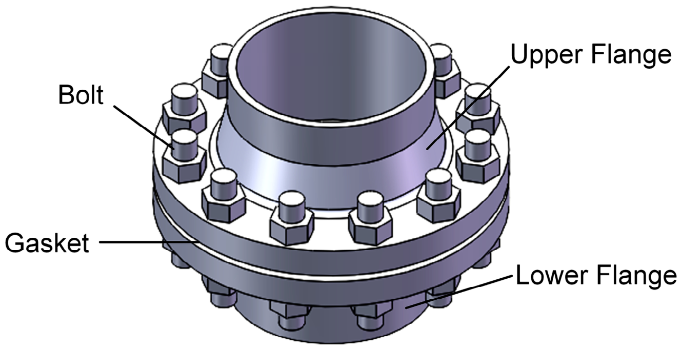
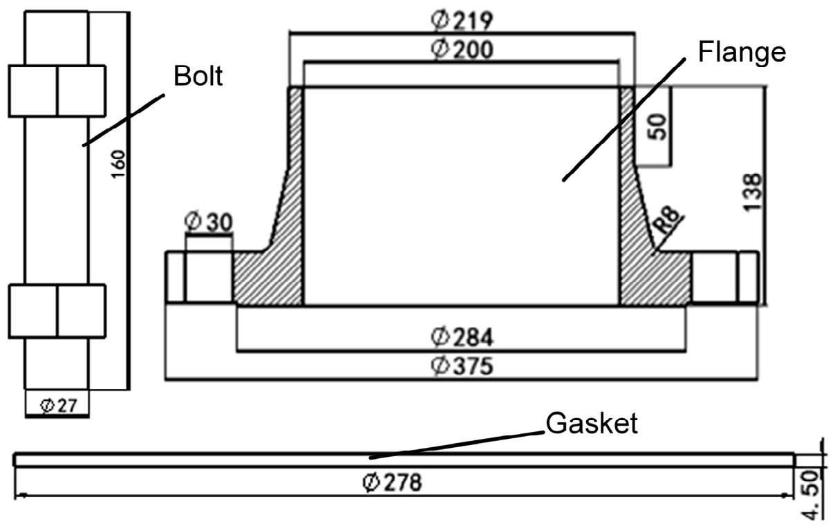
The study object is a DN200 PN40 weld-neck (WN) flange–bolt–gasket connection system (Figure 1), consisting of two flanges, one flexible graphite/304SS spiral-wound composite gasket, and 12 sets of M27 stud bolts and nuts uniformly distributed along the circumference. The principal geometric dimensions are annotated in Figure 2, and the key parameters are listed in

Table 1. Principal geometric parameters of the flange–bolt–gasket system.

Category	Parameter	Symbol	Value
Flange	Nominal diameter/Nominal pressure	DN/PN	200 mm/4.0 MPa
Flange	Pipe inner/outer diameter	$d_i/d_o$	φ200/φ219 mm
Flange	Flange outer diameter	D	φ375 mm
Flange	Bolt hole circle diameter	K	φ320 mm
Flange	Bolt hole diameter/quantity	$d_h$/n	φ30 mm/12
Flange	Total flange height/neck fillet radius	H/R	138 mm/8 mm
Gasket	Inner/outer diameter (baseline)	—	φ230/φ278 mm
Gasket	Width/thickness	b/t	24/4.5 mm
Bolt	Stud/nut specification	—	M27 × 160 double-end stud/M27 nut

.

The flange–bolt–gasket system exhibits strict 12-fold rotational symmetry in the circumferential direction. The 12 M27 studs uniformly distributed along the circumference form a cyclic symmetry group C₁₂ of order 12, whose generator is the 30° rotation operator about the z-axis. Application of the cyclic symmetry simplification requires that the geometry, material properties, boundary conditions, and loads simultaneously satisfy C₁₂ symmetry: in this study, the bolt holes and studs are uniformly distributed circumferentially, the materials are isotropic, the external loads (internal pressure, equivalent tensile stress, and convective heat transfer) and the temperature field are all axisymmetric about the z-axis, and the pretension is applied at the mid-shank of each stud with equal magnitude. All of these conditions are satisfied.

Under these conditions, the displacement field $\mathrm{u}\left(\mathrm{r},\mathrm{\theta },\mathrm{z}\right)$ in the cylindrical coordinate system satisfies the periodic constraint:

$$\mathrm{u}\left(\mathrm{r},\mathrm{\theta }+\mathrm{\alpha },\mathrm{z}\right)=\mathrm{R}\left(\mathrm{\alpha }\right)·\mathrm{u}\left(\mathrm{r},\mathrm{\theta },\mathrm{z}\right)$$

(1)

where $\mathrm{\alpha }=30°$ and $\mathrm{R}\left(\mathrm{\alpha }\right)$ is the second-order rotation tensor for a 30° rotation about the z-axis. This constraint is equivalent to requiring that the displacements of corresponding nodes on the high and low sector boundaries be identical in the cylindrical coordinate system. The finite element modeling methodology for symmetric bolted flange connections has been validated in the literature [31], and is consistent with the FEM approach for leakage prediction in gasketed flange connections [32]. In ANSYS Workbench, this constraint is imposed via the Cyclic Region function under the Symmetry branch, with the solver automatically establishing multi-point constraint equations for the low–high boundary node pairs.

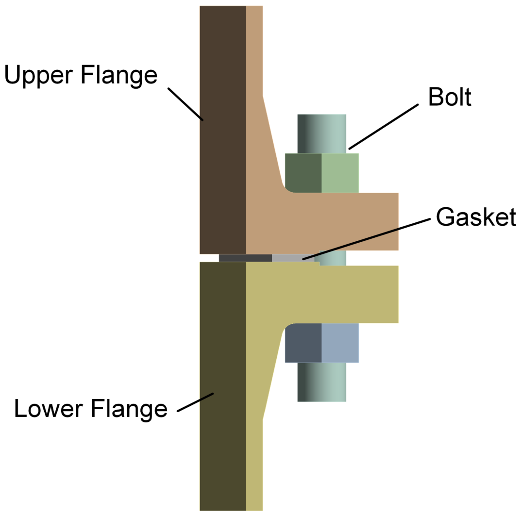
As shown in Figure 3, a 1/12 periodic sector is adopted as the finite element domain. Mid-plane mirror symmetry (the geometric reflection symmetry about the gasket mid-plane) was not exploited, primarily because the bolt pretension load is applied at the mid-shank of the stud, requiring the full bolt shank to be retained in order to avoid the localized stress disturbance that would otherwise be introduced at the pretension cross-section by an artificial mid-plane cut.

The 1/12 periodic-sector model assumes ideal $C_{12}$ cyclic rotational symmetry. In service, this symmetry is broken by bolt-by-bolt preload scatter under torque-controlled tightening (typically ±10–15% [33]), flange-face waviness within manufacturing tolerance, and external bending and shear loads transmitted through the connected piping. The $p_{min}$, ${\sigma }_{bolt}$, and bolt-force values reported here, and the optimized design (F = 59,942 N, b = 19.00 mm), should therefore be interpreted as ideal-symmetry averages around the circumference rather than worst-case local values; quantifying the worst-case local degradation requires a full-360° model and is identified as a natural direction for follow-on work.

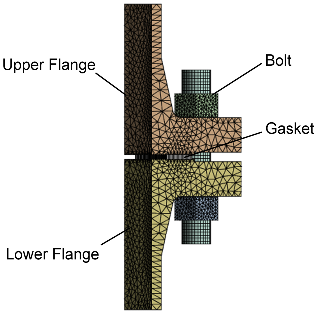
Since gasket width b is treated as a design variable in Section 4, a parametric strategy of fixed outer diameter and adjustable inner diameter is adopted: the gasket outer diameter is fixed at φ278 mm, and the inner diameter is varied to achieve b ∈ [19, 29] mm. The finite element mesh was generated in ANSYS Mechanical; the main body uses second-order tetrahedral elements SOLID187 with a global mesh size of 5 mm, while the gasket uses dedicated Gasket elements INTER194 with one layer retained through the thickness and an in-plane size of 1.3 mm. The model contains approximately 140,000 nodes in total (Figure 4); mesh independence verification is presented in Section 2.5.

2.2. Material Properties

The flange body is ASTM A105 carbon steel [34], the bolts and nuts are ASTM A193 B7 alloy steel [35], and the gasket is a 304 stainless steel/flexible graphite spiral-wound composite gasket [36]. Temperature-dependent material properties are adopted for the flange, bolts, and nuts (

Table 2. Temperature-dependent material properties of ASTM A105 flange.

Temperature (°C)	Thermal Expansion Coefficient (×10−6 °C−1)	Young’s Modulus (MPa)	Thermal Conductivity (W·m−1·°C−1)
15	11.5	203,000	60.5
100	12.7	198,000	58.0
200	13.8	192,000	52.8
300	14.9	185,000	47.9

and

Table 3. Temperature-dependent material properties of ASTM A193 B7 bolts and nuts.

Temperature (°C)	Thermal Expansion Coefficient (×10−6 °C−1)	Young’s Modulus (MPa)	Thermal Conductivity (W·m−1·°C−1)
15	11.2	204,000	42.4
100	11.9	199,000	42.2
200	12.5	193,000	40.5
300	13.1	187,000	38.0

), with a density of 7850 kg/m³ and a Poisson’s ratio of 0.30. The gasket is a nonlinear porous composite whose constitutive behavior is represented by a compression–stress curve [16] (

Table 4. Compression curve of the gasket at various temperatures.

Compression (mm)	15 °C (MPa)	100 °C (MPa)	200 °C (MPa)	300 °C (MPa)	400 °C (MPa)
0	0	0	0	0	0
0.2	6.4	5.8	5.4	4.3	3.8
0.4	15.2	13.2	12.1	10.7	9.1
0.8	48.9	44.5	40.4	37.2	34.9
1	78.7	74.1	68.3	63.3	59.7
1.1	105.6	99.3	93.5	87.5	82.4
1.2	140.1	133.2	125.8	117.4	112.5
1.3	185.6	176.3	166.1	156.9	149.2

).

It should be noted that Table 4 reports only the monotonic loading branch of the gasket constitutive behaviour. Spiral-wound gaskets are known to exhibit hysteretic load–compression behaviour, and the INTER194 element implementation in this study assigns the unloading branch a default linear stiffness equal to the secant elastic modulus of the upper loading segment. This is a conservative idealisation for spiral-wound gaskets, whose actual unloading stiffness has been reported to be approximately 5–10 times the initial loading tangent stiffness [10]. To quantify the resulting sensitivity for the present sealing problem, the Step-2 spring-back $\delta$ ≈ 0.02 mm under the baseline load combination, propagated through the literature-supported unloading-to-loading stiffness ratio, yields an upper-bound deviation of $p_{min}$ smaller than 0.4 MPa (below 1.5% of the baseline 28.70 MPa value), which lies below the resolution of the optimisation indicators and does not alter the ‘inner-loose, outer-tight’ failure mechanism conclusion or the recommended design point. The gasket effective thermal conductivity was set to $k_g=3.5 \mathrm{W}·{\mathrm{m}}^{-1}·{\mathrm{K}}^{-1}$, taken as a representative literature value for stainless-steel-strip/flexible-graphite spiral-wound composites [1]; a ±20% variation in $k_g$ changes the gasket centroidal temperature by less than 3 K and the Step-3 $p_{min}$ by less than 0.2 MPa. Furthermore, the experimental loading curve terminates at 185.6 MPa due to the test-rig capacity reported in [16]; for the $p_{\mathrm{m}\mathrm{a}\mathrm{x}}\le 210$ MPa crush-prevention constraint check used in the optimisation, a monotonic upper-bound extrapolation along the final loading tangent was applied as a conservative envelope, which is an order of magnitude tighter than the achieved constraint value and therefore safe in practice.

2.3. Steady-State Thermal–Structural Sequential Coupling

A steady-state thermal–structural sequential one-way coupling strategy was adopted [18,37]: a steady-state thermal analysis was first performed in the ANSYS Steady-State Thermal module to obtain the system temperature field, which was then imported as a body load into the Static Structural module for structural analysis. All finite element analyses reported in this study were performed in ANSYS Workbench release 2024 R1. The rationale for this one-way coupling is that, under steady-state conditions, the structural deformation (maximum axial displacement approximately 0.5 mm) is less than 0.13% of the flange characteristic dimension (375 mm), making its feedback effect on the thermal boundary conditions negligible; temperature-dependent material behavior is fully accounted for in the structural analysis through the temperature-dependent material library [38].

Thermal boundary conditions: a fixed wall temperature of 300 °C was applied to all inner wall surfaces of the flange; natural convection was applied to the outer surfaces and exposed bolt-and-nut surfaces, with a convection coefficient of h = 25 W/(m²·K) and an ambient temperature of 22 °C. The solver used the ANSYS default sparse direct method, with a thermal residual convergence criterion of less than 0.5%.

The value h = 25 W/(m²·K) is an effective combined heat-transfer coefficient that lumps natural convection together with the surface-radiation contribution. For pure natural convection over vertical and horizontal steel surfaces at the present outer-surface temperature range (approximately 200–270 °C), the textbook convective coefficient typically lies in the 5–10 W/(m²·K) range. The linearized radiative coefficient $h_{\mathrm{r}\mathrm{a}\mathrm{d}}$ = $\epsilon \sigma$($T_s^2+T_a^2$)($T_s$ + $T_a$), with an oxidized-steel emissivity $\epsilon \approx 0.85$ and the present temperature levels, evaluates to between 10 and 18 W/(m²·K), so the combined effective coefficient naturally falls in the 15–28 W/(m²·K) range; h = 25 W/(m²·K) is a conservative engineering midpoint within this band. A sensitivity check using a lumped-parameter energy balance shows that doubling h to 50 W/(m²·K) would lower the bolt-and-nut mean temperature by less than 10 °C, change the Step-3 bolt axial force by less than 3%, and shift $p_{min}$ less than 0.5 MPa, all of which are below the resolution of the optimization indicators.

The structural analysis was performed in the Static Structural module. A Fixed Support was applied to the bottom face of the lower flange to eliminate rigid-body motion, and a 30° Cyclic Symmetry constraint was applied to the sector side faces. Six contact pairs were defined for the 1/12 flange model (

Table 5. Contact pair settings.

Contact Pair	Type	Friction Coefficient	FKN	Algorithm	Behavior
Gasket ↔ Upper flange	Frictional	0.15	0.35	Augmented Lagrange	Symmetric
Gasket ↔ Lower flange	Frictional	0.15	0.35	Augmented Lagrange	Symmetric
Upper nut ↔ Upper flange	Frictional	0.15	0.10	Augmented Lagrange	Symmetric
Lower nut ↔ Lower flange	Frictional	0.15	0.10	Augmented Lagrange	Symmetric
Upper nut ↔ Stud shank	Frictional	—	—	MPC	—
Lower nut ↔ Stud shank	Frictional	—	—	MPC	—

), all set to symmetric behavior to improve numerical stability. The friction coefficient $\mu$ = 0.15 was taken as the midpoint of the steel-on-steel lubricated contact friction range (0.10–0.20) recommended by the ASME PCC-1 guidelines for bolted flange assembly [33]. The normal contact stiffness factor (FKN) values were selected with reference to the recommended range for rigid-to-flexible contact in the ANSYS contact parameter manual.

The use of a Fixed Support over the bottom annulus of the lower pipe stub is a conventional simplification adopted in flange–bolt–gasket finite-element studies that focus on the sealing region rather than on the pipeline boundary [39]. Although a fully fixed boundary nominally suppresses radial thermal expansion at the constrained face, all evaluation indicators of the present study ($p_{min}$ on the gasket contact face, $P_l+P_b$ on the stress classification line one wall thickness above the flange neck fillet, ${\sigma }_{bolt}$ on the bolt shank mid-section) are extracted at locations more than three pipe-wall thicknesses away from the constrained face. By the Saint-Venant principle, the artificial constraint stresses introduced at the bottom annulus decay exponentially over this characteristic distance, leaving a residual contribution to the monitored quantities below 1%. An order-of-magnitude estimate confirms this: the artificial radial thermal-constraint stress at the face itself, ${\sigma }_{\mathrm{f}\mathrm{a}\mathrm{c}\mathrm{e}}$ ≈ $E·\alpha ·\Delta T·\nu$ ≈ 185 GPa × 14.9 × 10⁻⁶ K⁻¹ × 280 K × 0.3 ≈ 230 MPa, attenuates to less than 3 MPa at the extraction locations, which is well below the resolution of the optimisation indicators. The Fixed Support boundary condition is therefore considered adequate for the present optimisation purpose; a fully realistic pipe-end load representation would require coupling to the upstream/downstream piping system and lies outside the scope of this study.

Although the friction coefficient is fixed at the ASME PCC-1 midpoint value $\mu =0.15$ in the primary analysis, the realistic assembly-induced spread of $\mu \in \left[0.10, 0.20\right]$ warrants a brief sensitivity comment. The bolt-up axial load in Step 1 is imposed via the ANSYS Bolt Pretension boundary condition rather than via threaded torque–tension conversion, so the resulting axial pretension is essentially independent of $\mu$. In Steps 2 and 3, the friction coefficient enters the model only at the gasket–flange and nut–flange contact pairs, where the loading is predominantly normal compression with limited tangential micro-slip. Under these conditions, the parametric studies of bolted flange–gasket assemblies reported by Murali Krishna et al. [15] and the contact-mechanics sensitivity analyses summarized by Croccolo et al. [40] show that varying $\mu$ across the [0.10, 0.20] range produces less than 5% variation in $p_{min}$ and the flange membrane-plus-bending stress $P_l+P_b$. These literature-supported bounds are an order of magnitude smaller than the trade-off magnitudes resolved by the optimization itself (+31.01% in $p_{min}$, −2.26% $P_l+P_b$), so the optimization conclusions are robust against realistic assembly-induced variability in friction. A dedicated full sensitivity sweep over, jointly with bolt-by-bolt preload scatter, would refine these qualitative bounds and is recommended as a follow-on study.

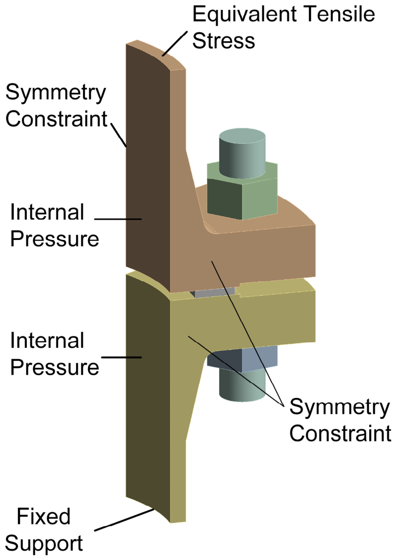
The loads applied to the flange–bolt system were introduced in three sequential steps corresponding to the actual service sequence. In Step 1 (bolt pretensioning), a Bolt Pretension load was applied at the mid-shank of the stud with a baseline value of F = 60,000 N to establish the initial sealing interface. In Step 2 (internal pressure loading), the Bolt Pretension was switched to the Lock state, an internal pressure of 4 MPa was applied to the flange inner wall, and an equivalent tensile stress of −20 MPa was applied to the upper annular end face of the upper flange to simulate the pipeline axial force. The negative sign in −20 MPa follows the ANSYS Pressure load convention, in which a negative value denotes an outward (tensile) traction acting on the loaded face along its outward normal; the magnitude is set so that the resulting axial traction (20.1 MPa) equals the design end thrust per unit pipe-section area (125.7 kN distributed over the pipe-section area of 6252 mm², giving 125.7 × 10³/6252 = 20.1 MPa), and the convention is therefore mathematically consistent with the tensile-positive sign convention adopted elsewhere in the manuscript for stress reporting. Internal pressure was not applied directly to the gasket inner-diameter (ID) cylindrical face. The omitted radial pressure load acts on a sectoral area of approximately π × 230 × 4.5/12 ≈ 271 mm² (gasket ID circumference times thickness, divided over the 30° cyclic-symmetry sector), giving a sectoral radial force of about 1.08 kN at 4 MPa. This radial load would press the gasket outward against the raised-face shoulder, but it does not directly contribute to the axial gasket–flange contact pressure that governs the primary sealing-performance indicator $p_{min}$. An order-of-magnitude bound is obtained by treating the omitted radial load as an additional overturning moment about the gasket mid-thickness; the resulting bending-stress contribution to $p_{min}$, of order 6 M/(b² × arc) with M = $F_r$ × t/2 ≈ 2.43 N·m, b = 24 mm and arc length $r_i$ × π/6 ≈ 60.2 mm, evaluates to approximately 0.42 MPa, below 1.5% of the baseline $p_{min}=28.70$ MPa and well below the resolution of the optimization indicators. The omission is therefore a well-bounded modeling simplification rather than a double-counting avoidance, and does not affect the engineering conclusions to within the resolution of this study. In Step 3 (temperature field import), the converged state from Step 2 was used as the starting point, and the steady-state temperature field was imported as a body load, with the Bolt Pretension remaining in the Lock state. The end state of Step 3 corresponds to the final mechanical response under the 300 °C service condition and serves as the reference state for subsequent extraction of evaluation indicators. The actual flange constraint types are diverse, and the boundary conditions are relatively complex in practice. Figure 5 schematically illustrates the boundary conditions of the 1/12 model.

This study is limited to a short-term sealing performance analysis under high-temperature steady-state conditions. Although the long-term creep–relaxation behavior of the gasket and bolts has an important influence on pretension evolution under actual service [11], the associated constitutive modeling and long-duration simulation fall outside the scope of this work and will be addressed separately in future studies.

It is nevertheless useful to indicate qualitatively how long-term creep and stress relaxation would shift the present steady-state predictions. In actual service, primary creep of the flexible-graphite filler in the spiral-wound gasket and stress relaxation of the A193 B7 bolts both reduce the gasket residual compressive stress monotonically with service time. Published creep–relaxation data for spiral-wound gaskets at 250–300 °C [11] indicate a typical 5–15% decay of the initial gasket seating stress within the first thousand operating hours, which would lower the inner-radius minimum contact pressure $p_{min}$ and erode part of the engineering margin (37.60 − 12.0 = 25.6 MPa above the $m·P$ sealing threshold) preserved in the optimized design under steady-state assumptions. Bolt stress relaxation operates in the same direction, redistributing axial load between the bolts and the gasket and further reducing $p_{min}$, with a magnitude of the same order as the gasket relaxation effect. The steady-state results obtained here therefore represent an upper bound on long-term sealing performance, and the optimized design should be re-examined under transient thermal cycling and creep–relaxation constitutive laws before being applied to extended-service conditions; the recommended $b=19 \mathrm{m}\mathrm{m}$ and the $F=\mathrm{59,942} \mathrm{N}$ pretension are expected to retain their relative ranking on the Pareto front, but the absolute improvement margins will inevitably shrink with service time.

2.4. Evaluation Indicator System

The flange–bolt–gasket system operating under high-temperature steam conditions is subject to three failure modes: gasket sealing failure, flange body cracking, and bolt yielding. To systematically evaluate these risks, an evaluation indicator framework encompassing both sealing performance and structural safety was established [41] (

Table 6. Evaluation indicator framework.

Indicator	Category	Criterion	Physical Significance
$p_{min}$	Objective ①	Maximize	Lower bound of sealing reliability
$P_l+P_b$	Objective ②	Minimize	Flange structural safety
$p_{max}$	Constraint ①	≤210 MPa	Gasket crush prevention
${\sigma }_{bolt}$	Constraint ②	≤580 MPa	Bolt yielding prevention
$p_{min}$	Constraint ③	≥12 MPa	ASME minimum seating stress (m·P)
$P_l+P_b$	Constraint ④	≤186 MPa	ASME VIII-2 1.5S limit
$C_u$	Auxiliary	—	Contact pressure uniformity
$S_f$	Auxiliary	≥1.0	Sealing margin

); all indicators are extracted at the end state of Step 3.

Four indicators are defined for sealing performance. The minimum gasket contact pressure $p_{min}$ characterizes the bearing state at the weakest sealing location; since sealing failure typically initiates where contact pressure is lowest, maximizing $p_{min}$ is adopted as one of the primary optimization objectives. The maximum contact pressure $p_{max}$ is used to control the risk of local gasket crushing, with the requirement $p_{max}\le 210$ MPa. The contact pressure uniformity coefficient $C_u$ $=$ $p_{min}/p_{avg}$ serves as an auxiliary indicator characterizing the uniformity of pressure distribution along the sealing surface. The sealing margin $S_f$ $=$ $p_{min}/\left(m·P\right)$ is defined in accordance with the m–y method in ASME VIII-1 Mandatory Appendix 2 [42], with the requirement $S_f$ ≥ 1.0:

$${\mathrm{S}}_{\mathrm{f}}={\displaystyle \frac{{\mathrm{p}}_{min}}{\left(\mathrm{m}·\mathrm{P}\right)}}$$

(2)

where m is the gasket factor, taken as 3.0 in this study, and P is the fluid internal pressure, taken as 4 MPa.

It should be noted that the use of the $m·P$ threshold as a sealing constraint follows the classical ASME VIII-1 Mandatory Appendix 2 procedure, which the Introduction of this study itself acknowledges as a simplified screening approach rather than a leakage-rate criterion. Within the present study, $p_{\mathrm{m}\mathrm{i}\mathrm{n}}\ge m·P$ is therefore adopted purely as an optimisation screening constraint and not as a formal leakage qualification. A more rigorous evaluation would require a leakage-rate framework such as the Pressure Vessel Research Council (PVRC) tightness-class methodology developed from Room Temperature Tightness Test (ROTT) data [43], or the leakage correlation models for spiral-wound gaskets and gasketed flange joints proposed by Jaszak and co-workers [4,32]. Replacing the $m·P$ screening with such a leakage-rate-based criterion would refine the absolute admissible level of $p_{min}$ and is a recommended extension of the present methodology.

Two indicators are defined for structural safety. The flange primary membrane-plus-bending stress $P_l+P_b$ is evaluated by stress linearization along a stress classification line (SCL) located approximately one wall thickness above the flange neck fillet, in accordance with the ASME VIII-2 Part 5 stress categorization method [42]; the allowable limit is 1.5S = 186 MPa, and this quantity is also adopted as the minimization objective in multi-objective optimization. The maximum equivalent bolt stress ${\sigma }_{bolt}$ is taken as the global maximum von Mises stress, with an allowable limit of 580 MPa, serving as a hard constraint throughout the optimization. ${\sigma }_{bolt}$ is a contact- and thread-region peak quantity; its mesh convergence across M1–M5 is verified in Section 2.5 (M4–M5 deviation 1.07%). For comparison with code-aligned working-stress limits, the nominal shank stress ${\sigma }_{shank}$ = F/$A_s$ of the M27 × 160 stud ($A_s$ = 459.4 mm² per ISO 898-1 [44]) at F = 60,000 N is 130.6 MPa, well below the ASME PCC-1 Appendix M target of 0.5 ${\sigma }_y$ = 290 MPa for SA-193 B7 at 300 °C [33]. ${\sigma }_{bolt}$ is retained as the operational constraint as a conservative upper-bound surrogate; at the recommended design point both criteria hold with substantial margin (${\sigma }_{bolt}$ = 471.98 MPa, ${\sigma }_{shank}$ = 130.5 MPa), providing a dual acceptance basis.

It is worth clarifying that the membrane-plus-bending stress $P_l+P_b$ evaluated in this study is extracted at the Step-3 end state, which already includes the steady-state thermal field. Under ASME VIII-2 Part 5, thermal-gradient and differential-expansion stresses are formally classified as secondary (Q) stresses and belong in a $P+Q$ assessment against the shake-down limit $S_{PS}$ (=3 $S_m$ per ASME BPVC VIII-2 Part 5) rather than in the 1.5S primary check. The use of $P_l+P_b\le 1.5S$ against the Step-3 stress in this study is therefore best understood as a combined-load engineering metric for surrogate construction and optimisation screening, lumping mechanical and thermal contributions into a single scalar, rather than as a formal code assessment. A formal $P+Q$ vs. $S_{PS}$ shake-down check would require separating the mechanical-only and mechanical-plus-thermal end states and is outside the scope of the present optimisation study; it represents a recommended follow-on activity for any subsequent code-qualification analysis of the recommended design point.

2.5. Mesh Independence Verification

Mesh independence verification was conducted under the baseline condition (F = 60,000 N, b = 24 mm, fluid temperature 300 °C), with $p_{min}$ as the primary monitor and $p_{avg}$ as the secondary monitor. Five mesh schemes, M1–M5, were designed (

Table 7. Mesh independence verification schemes.

Scheme	Global Size (mm)	Gasket–Flange Contact (mm)	Nut–Flange Contact (mm)	Nut–Stud Contact (mm)	Flange Fillet (mm)
M1	8	2.0	2.2	4.5	4.5
M2	6.5	1.7	2.0	4.0	4.0
M3	5	1.3	1.5	3.0	3.0
M4	4	1.0	1.2	2.5	2.5
M5	3	0.8	1.0	2.0	2.0

), with node counts ranging from 61,000 to 251,000. The relative error was defined with reference to the finest mesh M5:

$${\mathrm{\epsilon }}_{\mathrm{i}}=\left|{\displaystyle \frac{\left({\mathrm{p}}_{\mathrm{m}\mathrm{i}\mathrm{n}},\mathrm{i}-{\mathrm{p}}_{\mathrm{m}\mathrm{i}\mathrm{n}},\mathrm{M}5\right)}{{\mathrm{p}}_{\mathrm{m}\mathrm{i}\mathrm{n}},\mathrm{M}5}}\right|\times 100\%$$

(3)

where ${\epsilon }_i$ is the relative error of mesh scheme $i$, $p_{min}, i$ the minimum gasket contact pressure of scheme $i$, and $p_{min}$, M5 is the reference value from the finest mesh.

As shown in

Table 8. Mesh independence verification results.

Scheme	Node Count	${\mathit{p}}_{\mathit{m}\mathit{i}\mathit{n}}$ (MPa)	${\mathit{p}}_{\mathit{a}\mathit{v}\mathit{g}}$ (MPa)	${\mathit{\sigma }}_{\mathit{b}\mathit{o}\mathit{l}\mathit{t}}$ (MPa)
M1	60,962	28.669	31.947	370.96
M2	82,534	28.687	31.962	417.44
M3	143,849	28.700	31.972	476.98
M4	186,442	28.710	31.979	486.24
M5	251,022	28.713	31.982	491.52

, the relative errors of $p_{min}$ across all five schemes are below 0.16%, well within the 2% convergence threshold commonly adopted in engineering practice, and the monitored quantity exhibits a monotonically converging trend with increasing node count. ${\sigma }_{bolt}$ was additionally re-evaluated for all five schemes (Table 8, fifth column): the relative deviation from M5 decreases monotonically and reaches the 2% convergence threshold by M4 (M4–M5 deviation 1.07%); the working mesh M3 retains a 2.96% deviation in ${\sigma }_{bolt}$ and is therefore tighter on the primary sealing response $p_{min}$ (0.16%) than on the bolt-peak quantity. At the finest mesh M5, ${\sigma }_{bolt}$ = 491.52 MPa still retains an 88.48 MPa margin below the 580 MPa allowable, so the constraint-inactivity conclusions of Section 4.5 and Section 4.7 remain robust under mesh refinement, and ${\sigma }_{bolt}$ is retained as a conservative upper-bound surrogate consistent with the dual acceptance basis introduced in Section 2.4. Balancing computational accuracy and efficiency, mesh scheme M3 was selected for all subsequent simulations.

2.6. Experimental Comparison Validation

Complete high-temperature experimental data for DN200 PN40 flanges are not available in the open literature. Accordingly, a modeling methodology validation strategy was adopted: the reliability of the modeling approach itself was verified by reproducing published experimental results for a well-documented benchmark case (the 3-inch WN flange), rather than validating the point-by-point accuracy of the DN200 model. The methodological basis for this strategy is that the element types employed (SOLID187 + INTER194), the contact algorithm (Augmented Lagrange), the thermal–structural sequential coupling framework, and the material constitutive models are all scale-independent with respect to flange size; the reliability of the modeling methodology demonstrated on the benchmark case is therefore transferable to the present study object.

The benchmark case selected is the 3-inch WN flange with spiral-wound gasket connection experiment published by Omiya and Sawa at the 2009 ASME Pressure Vessel and Piping (PVP) Conference [8]. This reference provides complete geometric, material, and experimental data, and closely matches the present study in three core aspects: flange type (WN), gasket type (spiral-wound composite), and loading conditions (pretensioning + internal pressure + elevated temperature), making it a suitable benchmark for modeling methodology validation.

2.6.1. Bolt Load Validation

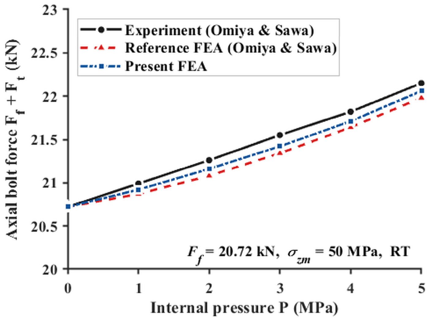
Under an initial pretension of $F_f$ = 20.72 kN (corresponding to ${\sigma }_{zm}$ = 50 MPa) and internal pressures ranging from 0 to 5 MPa, the bolt load $F_f+F_t$ was extracted as a function of internal pressure and compared against the experimental values reported by Omiya (Figure 6). The reproduced simulation predictions fall consistently between the experimental values and the original finite element analysis (FEA) results of Omiya, with a maximum relative error of 0.60% against the experimental data, outperforming the approximately 1.0% deviation between Omiya’s original FEA and the experiment.

2.6.2. High-Temperature Contact Pressure Distribution Validation

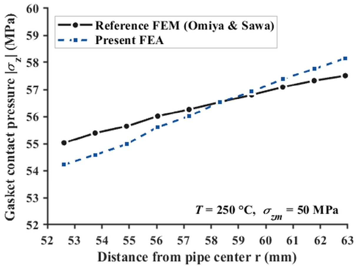
A steady-state temperature field of 250 °C—corresponding to the saturation temperature of 4 MPa steam in the Omiya–Sawa benchmark, in contrast to the 4 MPa/300 °C superheated-steam condition adopted for the DN200 PN40 study object—was further applied, and the radial gasket contact pressure distribution ${\sigma }_z$ was extracted and compared against the 250 °C FEM results reported by Omiya (Figure 7). The two curves show good agreement in distribution profile, pressure magnitude, and radial gradient, both exhibiting a monotonically increasing trend from the inner to the outer radius. The maximum relative error is 1.45%, and the mean relative error is 0.78% (

Table 9. Summary of benchmark validation errors (Level 1: bolt load vs. experiment; Level 2: high-temperature gasket contact pressure vs. reference FEM).

Validation Level	Compared Quantity	Condition	Reference Value	Simulated Value	Relative Error
Level 1	$F_f+F_t$	Ambient temperature, internal pressure 5 MPa	22.15 KN (experimental)	22.06 KN	−0.43%
Level 2	${\sigma }_z$ at inner radius	250 °C, internal pressure	55.39 MPa	54.59 MPa	−1.45%
Level 2	${\sigma }_z$ at outer radius	250 °C, internal pressure	57.51 MPa	58.15 MPa	+1.11%

).

All relative errors across both validation levels are below 1.5%, well within the 5% error threshold commonly adopted for engineering validation, confirming that the modeling methodology employed in this study is sufficiently reliable for predicting the high-temperature sealing performance of WN flange–spiral-wound gasket assemblies. The scale-independence of this methodology allows it to be directly transferred to the DN200 PN40 study object [9]. A similar three-dimensional nonlinear modeling approach has been successfully applied to bolted flange systems in aero-engine casings [45].

3. Thermal–Structural Coupled Analysis Under Baseline Operating Conditions

Based on the finite element model established in Section 2, this chapter performs a systematic thermal–structural coupling analysis under the design baseline condition (F = 60,000 N, b = 24 mm, fluid temperature 300 °C) to reveal the failure mechanisms and coupled physical response characteristics of the flange–bolt–gasket system under high-temperature steam service.

3.1. Temperature Field Distribution

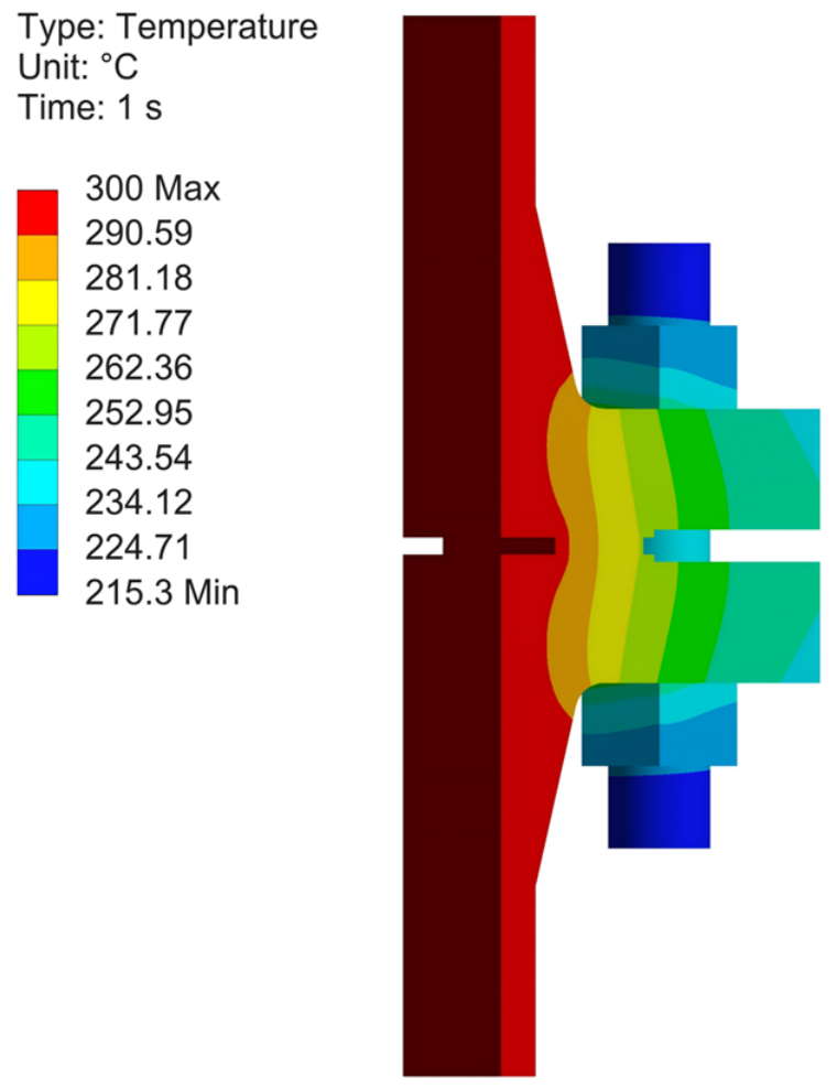
The steady-state thermal analysis was performed with a fixed temperature of 300 °C applied to all inner wall surfaces and natural convection applied to the outer surfaces (h = 25 W/(m²·K), ambient temperature 22 °C). The resulting steady-state temperature distribution is shown in Figure 8.

The temperature field exhibits a pronounced radial gradient from the inner-wall heat source to the outer dissipation surface. The flange inner wall is maintained at the fluid temperature of 300 °C and decreases monotonically in the radial direction. The bolts and nuts, located on the outer side of the flange, are significantly cooler than the flange body; the minimum temperature of 215.3 °C occurs at the stud head furthest from the flange, and the system mean temperature is 253.89 °C. The non-uniform temperature field produces two consequences: a peak-to-peak temperature difference of approximately 80 °C (flange inner wall 300 °C vs. stud-head minimum 215.3 °C) exists between the flange body and the bolts and nuts, and the differential thermal expansion between them directly affects the bolt axial force; the gasket is subjected to a non-uniform radial temperature distribution which, superimposed on the flange rotation effect, jointly governs the radial distribution of contact pressure [12].

3.2. Sealing Performance Evolution Under Three Loading Steps

3.2.1. Contact Pressure Distribution Evolution

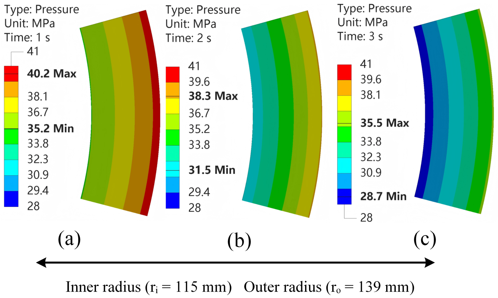
The gasket contact pressure distribution contours at the end of each loading step are shown in Figure 9, and the quantitative data are summarized in

Table 10. Sealing performance summary for the three loading steps under baseline conditions.

Loading Step	${\mathit{P}}_{\mathit{m}\mathit{i}\mathit{n}}$ (MPa)	${\mathit{P}}_{\mathit{m}\mathit{a}\mathit{x}}$ (MPa)	${\mathit{P}}_{\mathit{a}\mathit{v}\mathit{g}}$ (MPa)	Uniformity ${\mathit{C}}_{\mathit{u}}$	Bolt Axial Force (N)
Step 1	35.173	40.245	37.523	0.937	60,932
Step 2	31.480	38.257	34.688	0.907	69,317
Step 3	28.700	35.513	31.972	0.898	64,986

.

The gasket contact pressure decreases overall across the three loading steps: $p_{min}$ drops from 35.173 MPa to 28.700 MPa (−18.4%), and $p_{avg}$ decreases by 14.8%. The reduction from Step 1 to Step 2 is attributable to the radial back-pressure exerted by the internal pressure at the gasket inner radius, which partially offsets the compressive effect of pretensioning. The further reduction from Step 2 to Step 3 is jointly caused by flange thermal deformation and bolt stress relaxation under the high-temperature load. The contact pressure uniformity coefficient is defined as:

$$C_u={\displaystyle \frac{{\mathrm{p}}_{\mathrm{m}\mathrm{i}\mathrm{n}}}{{\mathrm{p}}_{avg}}}$$

(4)

where $p_{avg}$ is the mean contact pressure over the gasket sealing surface.

$C_u$ decreases from 0.937 in Step 1 to 0.898 in Step 3 (−4.2%), indicating that the high-temperature load exacerbates the radial non-uniformity of contact pressure. At the end of Step 3, $p_{min}$ = 28.7 MPa, well above the ASME VIII-2 minimum seating stress $m·P$ = 12 MPa, giving a sealing margin $S_f$ = 2.39; $p_{max}$ = 35.513 MPa is far below the crush strength limit of 210 MPa. The baseline condition satisfies the sealing requirements, while leaving room for further improvement through optimization.

3.2.2. Bolt Axial Force Evolution Mechanism

Table 10 shows that the bolt axial force follows a non-monotonic trend: 60,932 N (Step 1) → 69,317 N (Step 2, +13.8%) → 64,986 N (Step 3, −6.2%), yielding a net increase of +8.3% relative to the design pretension value F₀ = 60,000 N. The increase from Step 1 to Step 2 is driven by two mechanisms: the equivalent tensile stress of −20 MPa is transmitted through the flange to the bolt, producing additional axial tension; simultaneously, the radial back-pressure of the internal pressure at the gasket inner radius causes slight axial springback of the gasket, further stretching the bolt. Together, these effects produce a net increase of 8385 N. The decrease from Step 2 to Step 3 occurs because the flange body reaches a mean temperature of approximately 270 °C under the thermal field, significantly higher than the bolts and nuts at approximately 240 °C [10]; the resulting mean-to-mean temperature difference of approximately 30 °C (flange body mean ≈ 270 °C vs. bolts-and-nuts mean ≈ 240 °C, used here as the relevant quantity for the axial thermal-elongation balance) means that the axial thermal elongation of the bolts is less than that of the corresponding flange section, partially releasing the axial tension accumulated in Step 2. The final net increase of +8.3% indicates that the bolts remain in a high axial stress state during high-temperature service. The Step-1 extracted value 60,932 N (approximately +1.55% above the prescribed pretension $F_0$ = 60,000 N) corresponds to the bolt-shank reaction force averaged over a cross-section at the Bolt Pretension load application plane: once the pretension state is switched to the Lock state, the surrounding flange–nut–washer contact stack relaxes into a new static equilibrium in which the initially prescribed 60,000 N axial load is redistributed across the local elastic compliance of the threads, contact pairs, and flange seating, and the small ~1.55% residual is the converged equilibrium reaction rather than a deviation from the prescribed pretension.

3.2.3. Flange Rotation and the Inner-Loose, Outer-Tight Phenomenon

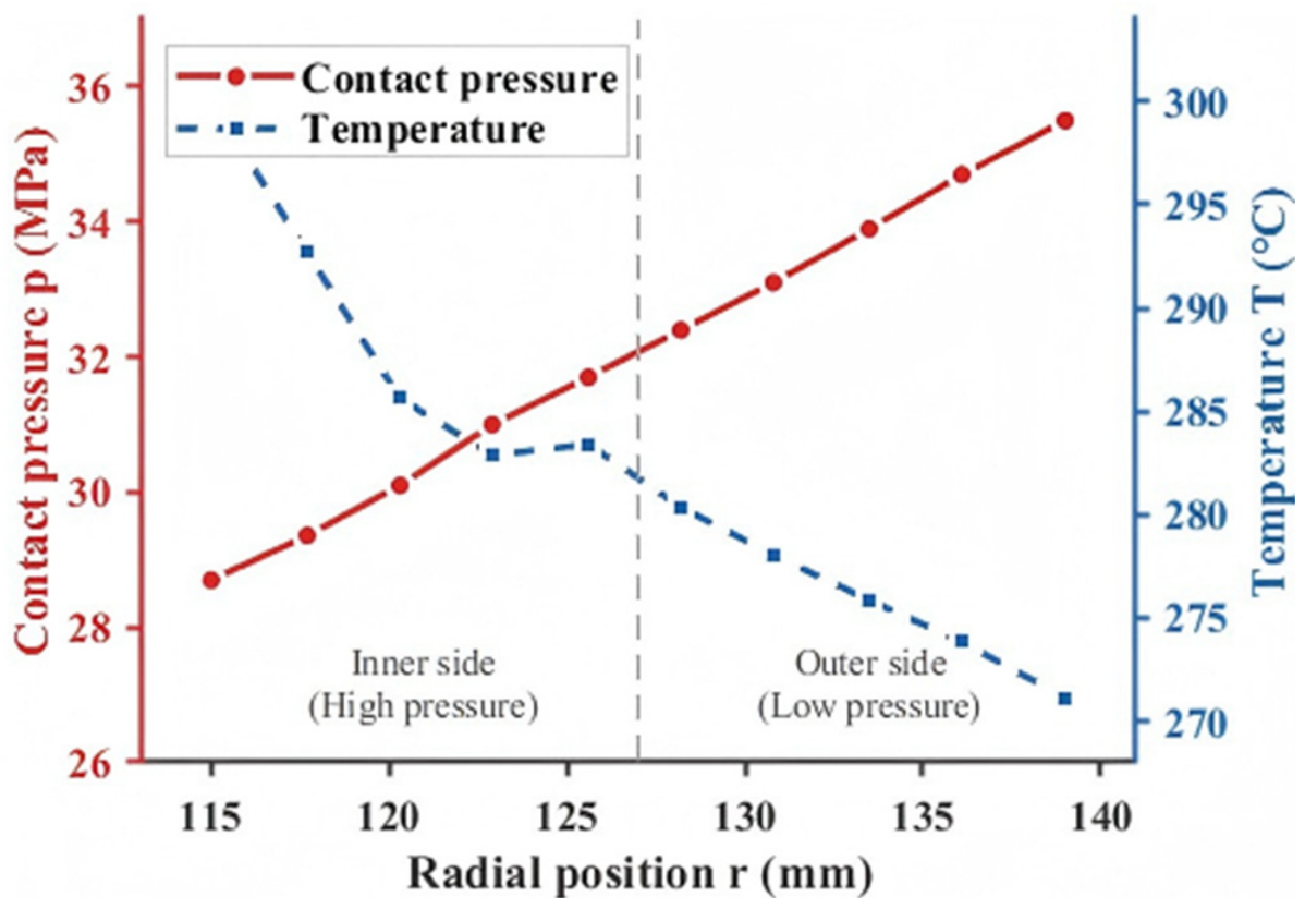
The radial distribution of gasket contact pressure under the Step 3 load is one of the most critical indicators of system sealing performance. Ten measurement points were uniformly distributed along the gasket radius (r ∈ [115.0, 139.0] mm); the contact pressure and temperature at each point are listed in

Table 11. Radial distribution of gasket contact pressure and temperature (Step 3, 300 °C condition).

Point	Radial Position r (mm)	Contact Pressure P (MPa)	Temperature T (°C)
1	115.0	28.70	300.00
2	117.7	29.36	292.69
3	120.3	30.10	285.64
4	122.9	31.00	282.88
5	125.6	31.70	283.41
6	128.2	32.40	280.37
7	130.8	33.10	278.04
8	133.5	33.90	275.86
9	136.1	34.70	273.84
10	139.0	35.50	271.13

, and the distribution curves are shown in Figure 10.

The contact pressure rises steadily from the inner to the outer radius, from 28.70 MPa to 35.50 MPa—a difference of 23.7%—while the temperature decreases overall in the same direction, from 300 °C to 271.13 °C (a net drop of 28.87 °C), with a minor non-monotonic fluctuation between points 4 and 5 in Table 11 (282.88 °C → 283.41 °C) that is attributable to local variations in contact thermal conductance with contact pressure rather than any reversal of the underlying radial gradient. Tighter compression at the outer radius and looser contact at the inner radius is what engineers call the inner-loose, outer-tight phenomenon [46], and it is the main failure mode in high-temperature flange sealing. It arises because the flange body bends about the hub fillet under the combined bolt pretension and internal pressure, tilting the sealing face away from the horizontal plane. The flange rotation angle θ is defined as:

$$\theta \approx {\displaystyle \frac{\left[u_y\left(r_{out}\right)-u_y\left(r_{in}\right)\right]}{\left(r_{out}-r_{in}\right)}}$$

(5)

where u y denotes the nodal axial displacement, and r in and r out are the inner and outer radii of the sealing face, respectively.

Based on the end-state simulation of Step 3, $u_y\left(r_{in}\right)$ = −0.34576 mm and $u_y\left(r_{out}\right)$ = −0.47486 mm; substituting into Equation (5) gives θ ≈ −0.00538 rad (−0.308°). The negative sign indicates that the flange sealing face tilts outward overall, with the outer radius sinking more than the inner radius, thereby imposing greater compressive displacement on the outer gasket while relatively relieving the inner gasket. The minimum contact pressure $p_{min}$ = 28.70 MPa occurs precisely at the inner radius at r = 115 mm, identifying this location as the critical sealing failure path and providing direct physical justification for adopting $p_{min}$ as the primary optimization objective in the subsequent multi-objective optimization.

3.3. Flange Stress Intensity Assessment

ASME VIII-2 Part 5 requires stress linearization assessment at critical cross-sections of pressure vessels, decomposing the true through-thickness stress distribution into a membrane stress $P_m$ (uniform component), a bending stress $P_b$ (linear component), and a peak stress (local component), each compared against the corresponding allowable limit.

$$P_m=\left({\displaystyle \frac{1}{t}}\right)·{\int }_0^t\sigma \left(x\right) dx$$

(6)

$$P_b=\left({\displaystyle \frac{6}{t^2}}\right)·{\int }_0^t\sigma \left(x\right)·\left({\displaystyle \frac{t}{2}}-x\right) dx$$

(7)

where σ(x) is the normal stress at a point along the stress classification line (SCL); t is the total length of the SCL path, 19.28 mm in this study; and x is the distance from the starting point along the SCL.

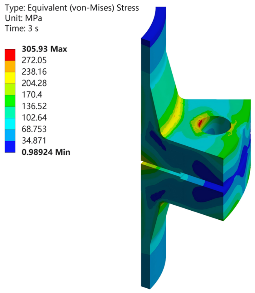
The combined membrane-plus-bending stress $P_l+P_b$ was computed automatically by the ANSYS stress linearization tool in accordance with ASME BPVC VIII-2 Part 5 Annex 5.A. The overall von Mises stress distribution of the flange under the Step 3 end state is shown in Figure 11.

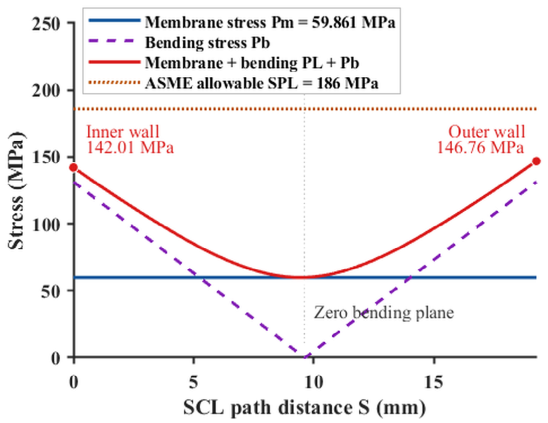
The maximum stress of approximately 305 MPa occurs in the contact loading zone near the bolt holes, which is a peak stress (F-type, per ASME VIII-2 Part 5 stress classification) local concentration and is therefore not used directly for strength assessment. Stress levels in the flange neck-to-transition region range from 102 to 170 MPa and constitute the region of concern for code assessment. The SCL was positioned in accordance with the recommended criteria of ASME VIII-2 Annex 5.A [47]: the SCL should be placed at a distance of one wall thickness from any stress concentration, oriented perpendicular to and spanning the full flange wall thickness. In this study, the SCL originates at one wall thickness (≈19 mm) above the flange neck fillet and extends radially to the outer wall, with a total path length of 19.28 mm. This location avoids the F-type peak stress at the fillet root and accurately captures the combined membrane-plus-bending stress state in the flange neck, in full conformance with the stress classification assessment procedure of ASME VIII-2 Part 5 [48]. The stress linearization results along the SCL path are shown in Figure 12.

Along the SCL path, the membrane stress $P_m$ = 59.86 MPa remains constant; the bending stress $P_b$ exhibits a typical antisymmetric V-shaped distribution; and the combined membrane-plus-bending stress $P_l+P_b$ shows a symmetric U-shaped profile, reaching its maximum at both ends (142.01 MPa at the inner wall end and 146.76 MPa at the outer wall end). The strength assessment based on these linearization results is presented in

Table 12. ASME VIII-2 stress intensity assessment results for the flange (reported here as an engineering combined-load metric for optimisation screening; not a formal $P+Q$ vs. $S_{\mathrm{P}\mathrm{S}}$ shake-down assessment, see Section 2.4).

Assessment Item	Criterion	Simulated Value (MPa)	Allowable Value (MPa)	Safety Margin
General membrane stress $P_m$	$P_m\le S$	59.86	124	2.07
Membrane-plus-bending stress $P_l+P_b$	$P_l+P_b\le 1.5S$	146.76	186	1.27

.

The allowable stress for A105 at 300 °C is S = 124 MPa (ASME II-D Table 5A), giving SPL = 1.5S = 186 MPa. Both indicators satisfy ASME VIII-2 requirements; however, the safety margin for $P_l+P_b$ (1.27) is notably smaller than that for Pm (2.07), indicating that bending stress is the dominant factor governing flange structural failure. In subsequent optimization, $P_l+P_b$ is treated both as a constraint and as the minimization objective in the multi-objective formulation.

3.4. Coupled Failure Mode Analysis and Necessity of Optimization

Synthesizing the results of Section 3.1, Section 3.2 and Section 3.3, the DN200 PN40 flange–bolt–gasket system operating at 300 °C exhibits three mutually coupled failure modes. Sealing failure, characterized by $p_{min}$ has a baseline value of 28.70 MPa and a sealing margin $S_f$ = 2.39, satisfying the ASME criterion; however, $p_{min}$ decreases continuously across all three loading steps. Flange cracking, characterized by $P_l+P_b$, has a baseline value of 146.76 MPa and a safety margin of 1.27, with bending stress as the dominant failure mode. Bolt yielding, characterized by ${\sigma }_{bolt}$, currently satisfies the yield strength requirement of A193 B7 at 300 °C (580 MPa), but ${\sigma }_{bolt}$ is highly sensitive to the pretension force F.

Significant trade-offs exist among the three failure modes: increasing F improves $p_{min}$ but simultaneously intensifies flange bending deformation, causing $P_l+P_b$ and ${\sigma }_{bolt}$ to rise in tandem; reducing gasket width b increases the contact pressure per unit area and shortens the bending moment arm of the flange, producing favorable effects on both $p_{min}$ and $P_l+P_b$. These complex multi-variable, multi-objective, multi-constraint trade-offs cannot be resolved by single-parameter adjustment and must be addressed through systematic multi-objective optimization with a global search over the design space. Accordingly, the multi-objective optimization problem is formulated as follows: F and b are taken as design variables; maximization of $p_{min}$ and minimization of $P_l+P_b$ are set as the two optimization objectives; and $p_{max}$ ≤ 210 MPa, ${\sigma }_{bolt}$ ≤ 580 MPa, $p_{min}$ ≥ 12 MPa, and $P_l+P_b$ ≤ 186 MPa are imposed as four constraints.

4. Surrogate Modeling and Multi-Objective Optimization

Section 3 identified three coupled failure modes—gasket leakage, flange cracking, and bolt yielding—in the DN200 PN40 flange–bolt–gasket system operating at 300 °C, providing a physical basis for multi-objective optimization. This chapter collects sample data based on a central composite design (CCD), constructs and comparatively evaluates second-order response surface (RSM) and Kriging surrogate models, conducts Sobol global sensitivity analysis, and finally employs NSGA-II to solve the Pareto front, applies TOPSIS to select the optimal compromise solution, and verifies the optimum by back-substitution into ANSYS.

4.1. Design of Experiments

4.1.1. Design Variables and Their Ranges

The flange–bolt–gasket system involves numerous design parameters. Design variables were selected in this study based on the following three criteria:

• Significant influence on the core evaluation indicators. A preliminary sensitivity screening of gasket thickness t was conducted at three pretension levels (F = 45,000, 60,000, and 75,000 N), with t set to 3.2, 4.8, and 6.4 mm around the nominal value of 4.5 mm. The maximum relative variations were below 0.5% in $p_{min}$, 1.0% in $P_l+P_b$, and 0.2% in bolt axial force—all substantially smaller than the main effects of F and b. Accordingly, the nominal value t = 4.5 mm was adopted for all primary simulations with confidence.
• Engineering adjustability. Bolt pretension F and gasket width b are parameters that can be directly controlled during design and assembly—F is precisely regulated via a torque wrench or hydraulic tensioner, and b is specified through standard gasket selection.
• Consistency with the coupled failure mechanism. The “inner-loose, outer-tight” failure mechanism identified in Section 3 is directly governed by flange rotation θ, which is primarily determined by F (driving the bending moment) and b (governing the moment arm). These two variables are therefore the most physically meaningful design variables within this mechanistic framework.

Based on the above criteria, F and b were selected as design variables, while all other geometric parameters were fixed at their standard values for DN200 PN40 flanges. The range of F was determined according to ASME codes: the lower bound $F_{min}$ ≈ 45,000 N was calculated using the ASME VIII-1 Mandatory Appendix 2 m–y method [42], and the upper bound $F_{max}$ = 75,000 N was determined from the ASME II-D bolt allowable stress. The upper bound of b is constrained by the radial geometry of the flange raised face, giving $b_{max}$ = 29 mm, and the lower bound is $b_{min}$ = 19 mm. The design variable ranges are summarized in

Table 13. Design variable ranges.

Variable	Symbol	Lower Bound	Baseline	Upper Bound	Basis
Bolt pretension	F (N)	45,000	60,000	75,000	ASME VIII-1/II-D
Gasket width	b (mm)	19	24	29	Geometric constraint/uniformity

.

4.1.2. CCD Design

A face-centered central composite design (FC-CCD, α = 1) was employed, generating 9 sampling points for two variables at three levels. Three additional independent validation points V1–V3 were included, covering the lower-middle and upper-middle pretension ranges. The design matrix is given in

Table 14. CCD design matrix (9 training sample points + 3 independent validation points).

Type	ID	F (N)	b (mm)	x1	x2
CCD	C1 (corner)	45,000	19	−1	−1
CCD	C2 (corner)	75,000	19	+1	−1
CCD	C3 (corner)	45,000	29	−1	+1
CCD	C4 (corner)	75,000	29	+1	+1
CCD	A1 (axial)	45,000	24	−1	0
CCD	A2 (axial)	75,000	24	+1	0
CCD	A3 (axial)	60,000	19	0	−1
CCD	A4 (axial)	60,000	29	0	+1
CCD	M1 (center)	60,000	24	0	0
CCD	V1	52,000	21	−0.53	−0.60
CCD	V2	68,000	27	+0.53	+0.60
CCD	V3	55,000	26	−0.33	+0.40

. The coded variable transformation is defined as x₁ = (F − 60,000)/15,000 and x₂ = (b − 24)/5.

The use of the minimum FC-CCD configuration (2 variables × 9 sample points) is justified on three grounds:

• Finite element simulation is a deterministic numerical process in which identical inputs yield a unique output; no experimental randomness is present, and center-point replication provides no additional pure-error information. This practice is standard in surrogate modeling studies driven by deterministic simulations.
• The second-order RSM contains six parameters to be estimated; 9 sample points provide 3 residual degrees of freedom for residual analysis and significance testing. The regression F-statistic p-values for all responses are below 10⁻⁴, confirming overall model significance.
• The three independent validation points V1–V3, covering the lower-middle and upper-middle pretension ranges, serve as external accuracy assessors; they reflect the engineering predictive capability of the surrogate model more directly and objectively than the internal pure-error estimates obtained from center-point replication alone.

4.2. Surrogate Model Construction

4.2.1. Second-Order Response Surface Model (RSM)

The second-order RSM in the coded space includes linear, quadratic, and interaction terms:

$$\hat{\mathrm{y}}={\beta }^0+{\beta }^1{x}^1+{\beta }^2{x}^2+{\beta }^{11}{x}^{12}+{\beta }^{22}{x}^{22}+{\beta }^{12}{x}^1{x}^2$$

(8)

where x₁ = (F − 60,000)/15,000 and x₂ = (b − 24)/5, with x₁, x₂ ∈ [−1, 1] after coding; β denotes the regression coefficients to be estimated.

The model contains six parameters to be estimated. The nine CCD sample points were used to solve for the coefficients via ordinary least squares, β = (X^TX)⁻¹X^Ty, yielding 9 − 6 = 3 residual degrees of freedom. Separate regressions were performed for the four responses ($p_{min}$, $p_{max}$, $P_l+P_b$, and ${\sigma }_{bolt}$), and the resulting coefficients are listed in

Table 15. Second-order RSM regression coefficients (coded space).

Response	β0	β1	β2	β12	β11	β22
$p_{min}$	28.423	8.422	−7.332	−1.802	0.285	1.849
$p_{max}$	35.953	10.260	−6.675	−1.760	0.023	1.361
$P_l+P_b$	146.63	28.122	3.095	2.680	2.938	−0.242
${\sigma }_{bolt}$	477.45	96.045	−0.628	3.253	0.902	0.012

.

t-tests revealed that the first-order and interaction terms of F and b are significant for $p_{min}$ and $p_{max}$ (p < 0.05); the first-order and quadratic terms of F are significant for $P_l+P_b$ (p < 0.01), indicating a nonlinear amplification of flange stress with respect to pretension; for ${\sigma }_{bolt}$, only the first-order term of F is significant (p < 0.001), with p-values for all b-related terms exceeding 0.4, suggesting that ${\sigma }_{bolt}$ is essentially a linear function of F throughout the design space. This finding is independently confirmed by the Sobol analysis in Section 4.4.

The goodness-of-fit metrics for the four responses on the training set are listed in

Table 16. RSM goodness-of-fit summary.

Response	R2	Adj-R2	RMSE	F-Statistic	p-Value
$p_{min}$	0.9988	0.9967	0.5647	481.82	1.49 × 10−4
$p_{max}$	0.9994	0.9984	0.4317	981.71	5.12 × 10−5
$P_l+P_b$	0.9999	0.9998	0.3777	6798.45	2.81 × 10−6
${\sigma }_{bolt}$	0.9998	0.9995	1.8348	3290.89	8.36 × 10−6

, including the coefficient of determination R², the adjusted coefficient of determination Adj-R², the root mean square error (RMSE), and the p-value of the overall F-test.

As shown in Table 16, the Adj-R² values for all four responses exceed 0.996, and the overall F-test p-values are all below 1.5 × 10⁻⁴, confirming high overall model significance. The near-unity Adj-R² values for $P_l+P_b$ and ${\sigma }_{bolt}$ reflect the strongly linear dominant behavior of these two responses across the design space. The difference between R² and Adj-R² does not exceed 0.003 for any response, indicating that all six estimated coefficients make a substantive contribution to the fit and that no spurious R² inflation due to redundant parameters is present.

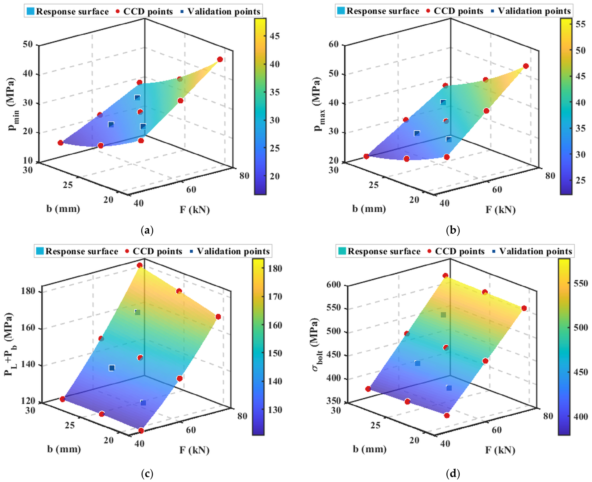
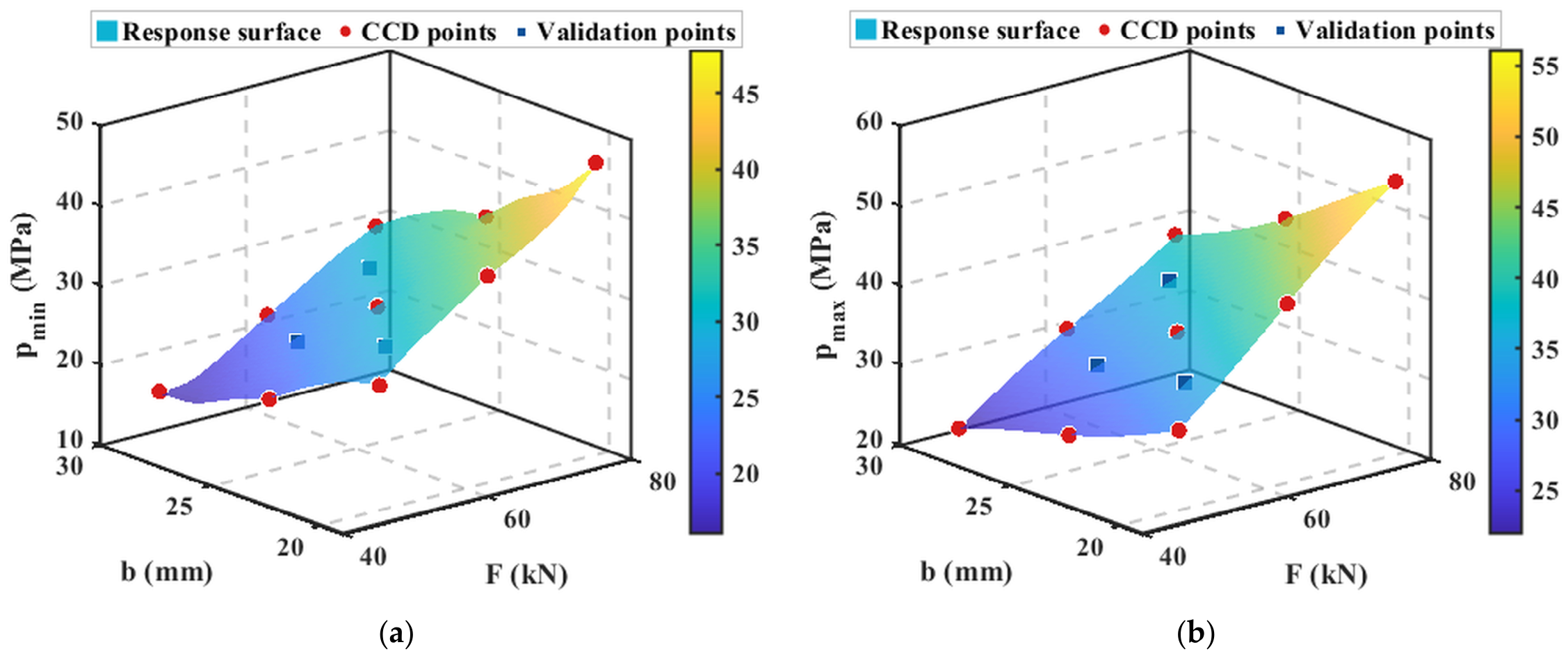
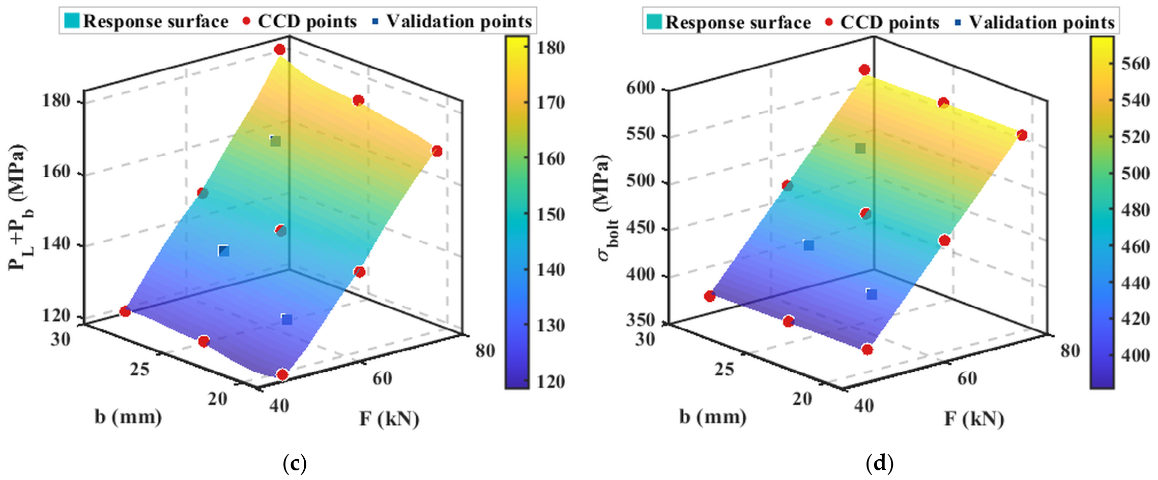
Figure 13 presents three-dimensional response surface plots for the four responses fitted by the second-order RSM, with red circles indicating CCD training points and blue squares indicating independent validation points.

As shown in Figure 13, all four response surfaces are smooth and continuous with no anomalous oscillations. The $p_{min}$ and $p_{max}$ surfaces increase monotonically with increasing F and decreasing b, consistent with the physical principle that higher pretension and narrower gasket width produce greater contact pressure per unit area. The $P_l+P_b$ and ${\sigma }_{bolt}$ surfaces are nearly flat in the b direction, in agreement with the finding in Table 15 that the b-related coefficients carry low statistical significance. Both the CCD training points (red circles) and the independent validation points (blue squares) lie close to the surfaces, providing a preliminary indication of the model’s predictive capability.

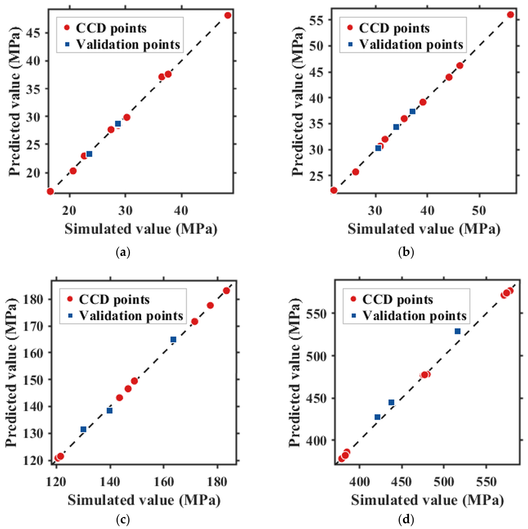
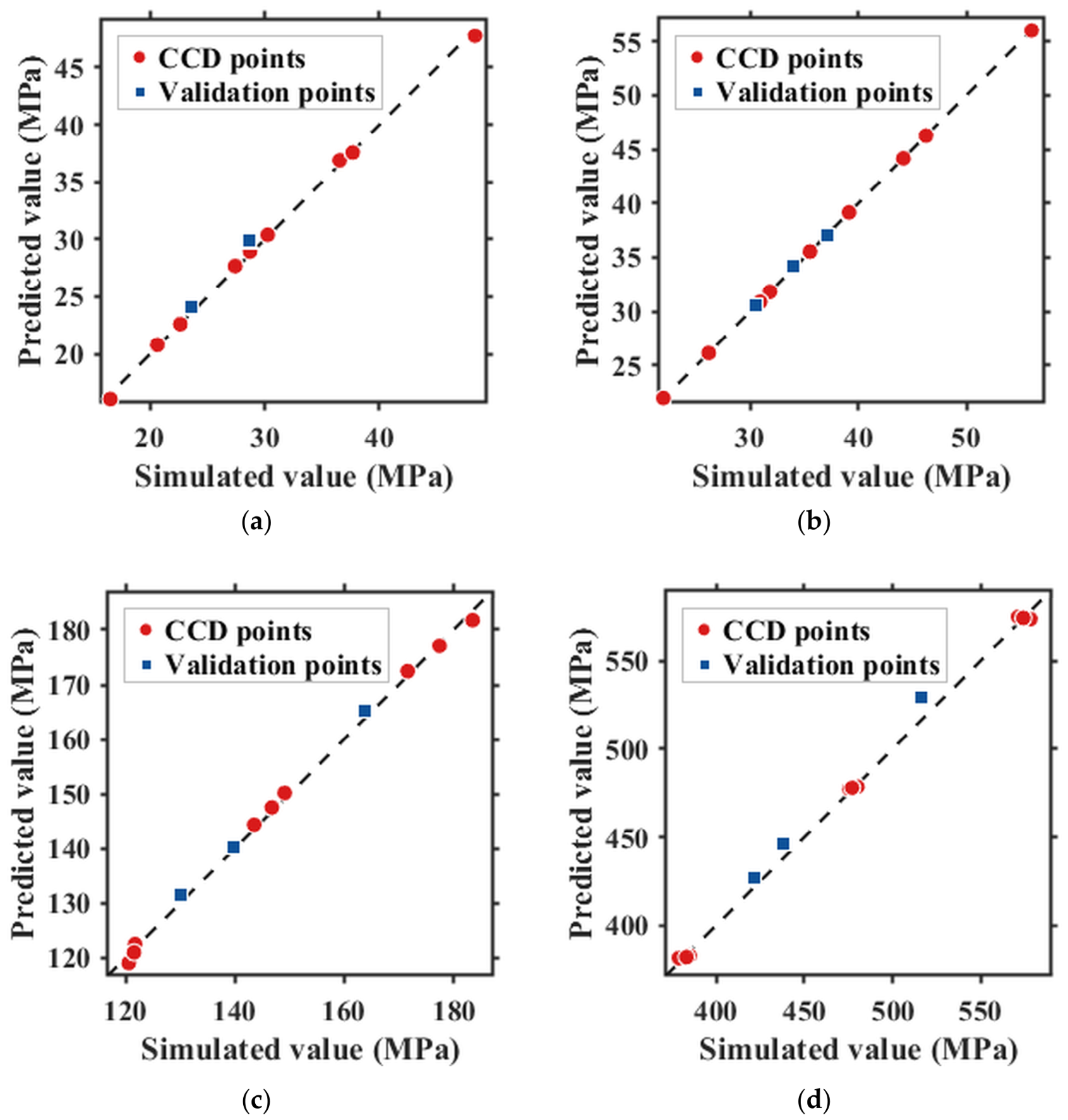
Figure 14 presents scatter plots comparing RSM predicted values against ANSYS simulated values for the four responses, with the dashed line representing the ideal prediction line y = x.

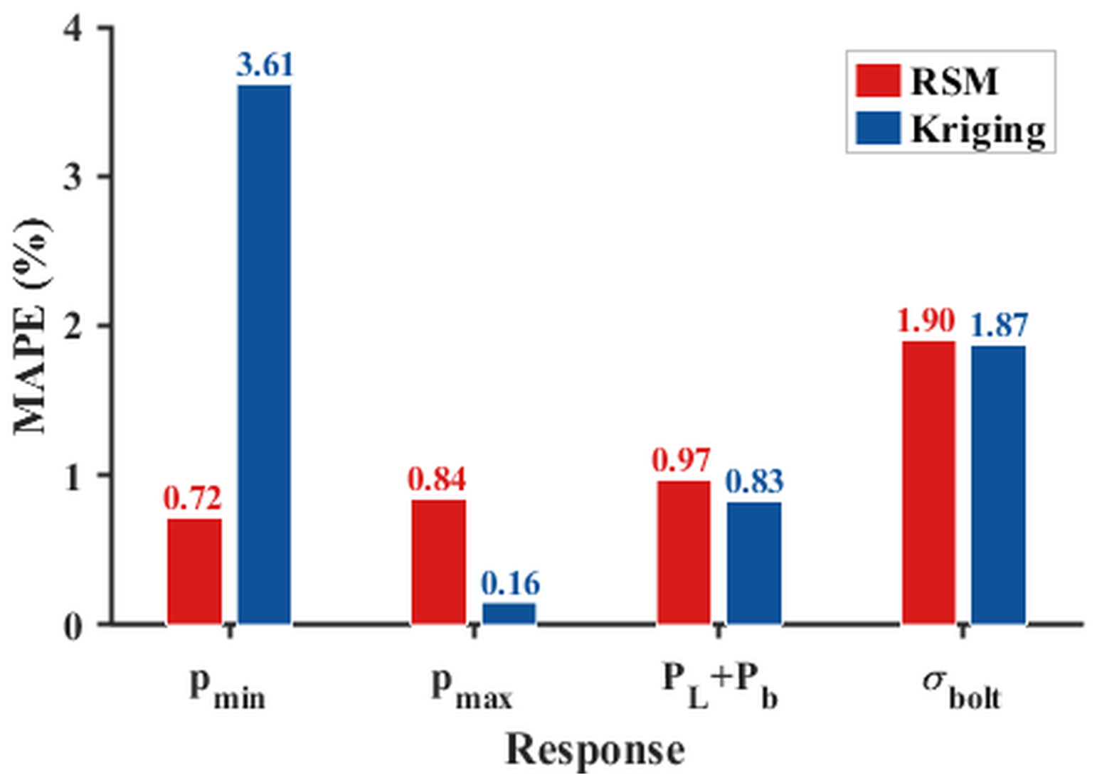
As shown in Figure 14, both training and validation points in all four subplots closely follow the y = x reference line. The validation set MAPEs are 0.72% ($p_{min}$), 0.84% ($p_{max}$), 0.97% ($P_l+P_b$), and 1.90% (${\sigma }_{bolt}$), all below 2%, indicating that the RSM exhibits no appreciable overfitting in either the interpolation or extrapolation regions.

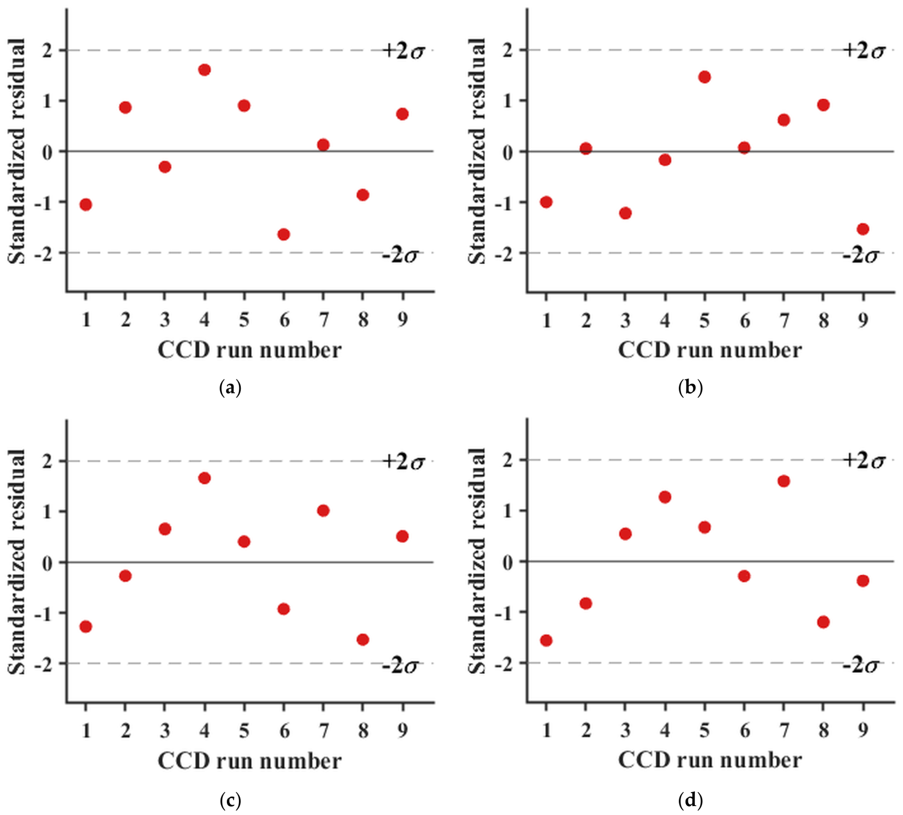
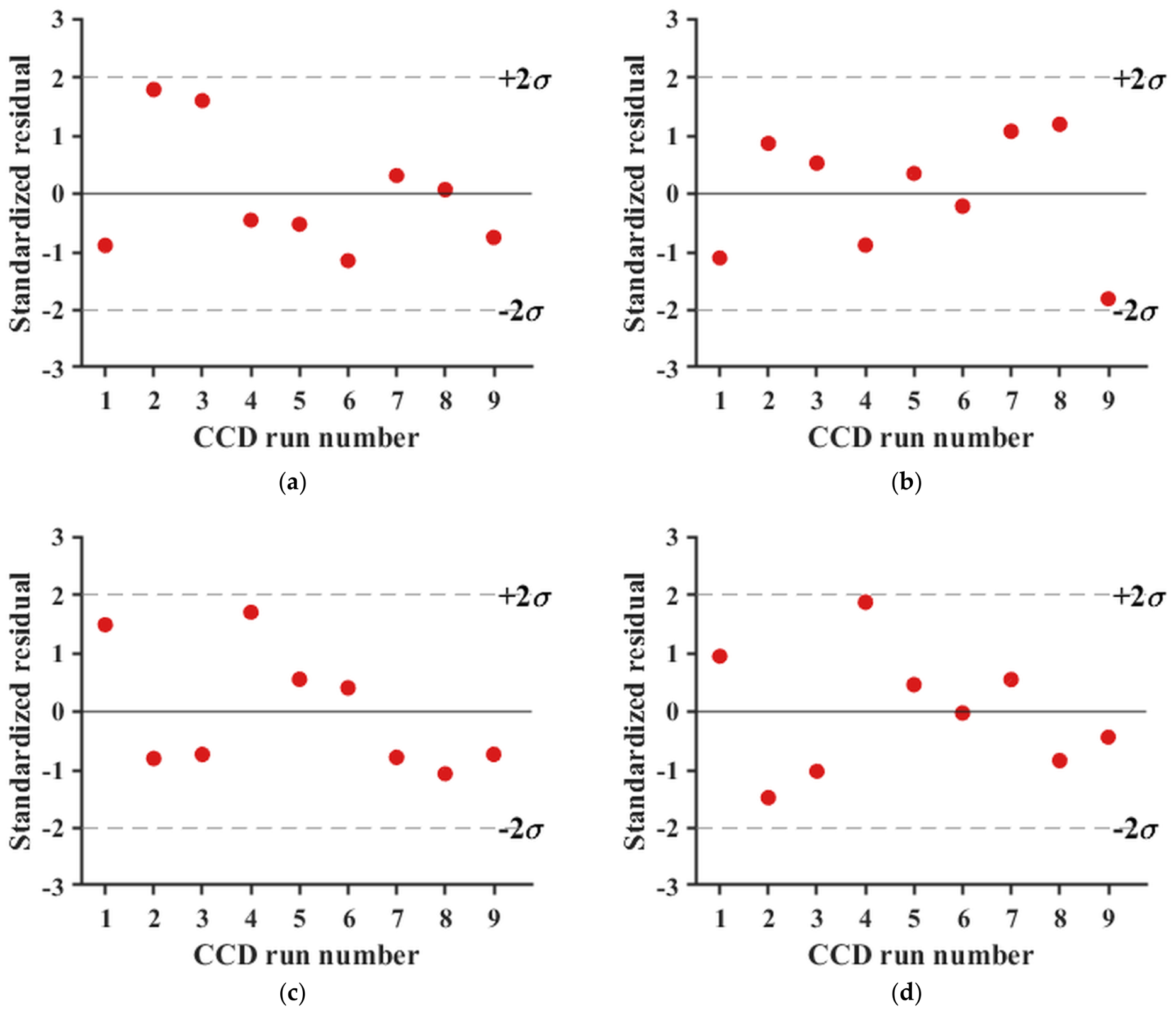
Figure 15 presents the standardized residual diagnostic plots for the RSM training set, with sample index on the horizontal axis, standardized residuals on the vertical axis, and dashed lines marking the ±2σ boundaries.

As shown in Figure 15, the standardized residuals of all nine training samples fall within the $\pm 2\sigma$ interval and exhibit no systematic upward or downward trend, indicating that the residuals approximately follow a zero-mean normal distribution. The second-order RSM model assumptions therefore hold within the design space of this study.

4.2.2. Kriging Surrogate Model

The Kriging model consists of a global trend term and a zero-mean Gaussian process:

$$\hat{\mathrm{y}}\left(x\right)=f{\left(x\right)}^{\mathrm{T}} \beta +Z\left(x\right)$$

(9)

$$R(x_{\mathrm{i}}, x_{\mathrm{j}})=\exp [-{\sum }_{\mathrm{k}} {\theta }_{\mathrm{k}}{(x_{\mathrm{i}\mathrm{k}}-x_{\mathrm{j}\mathrm{k}})}^2]$$

(10)

where f(x) is a linear basis function, Z(x) is a zero-mean Gaussian process, and θ_k are kernel hyperparameters estimated by maximum likelihood estimation (MLE).

A squared exponential kernel $R(x_{\mathrm{i}}, x_{\mathrm{j}})=exp(-{\sum }_{\mathrm{k}} {\theta }_{\mathrm{k}}{(x_{\mathrm{i}\mathrm{k}}-x_{\mathrm{j}\mathrm{k}})}^2)$ was adopted, with hyperparameters θ_k learned via maximum likelihood estimation (MLE). Although classical Kriging formulations can be configured to interpolate exactly through the training points, the fitrgp implementation used here jointly estimates a homoscedastic observation noise variance ${\sigma }_n^2$ (analogous to the nugget term in geostatistical Kriging) together with the kernel hyperparameters by default, so the surrogate is more precisely characterised as Gaussian process (GP) regression rather than exact interpolation [49]. The model was implemented in MATLAB R2024a using the fitrgp function with a linear basis function and a squared exponential kernel. The noise standard deviations ${\sigma }_n$ estimated by MLE (model.Sigma) are 1.53 MPa, 1.36 MPa, 2.21 MPa and 2.45 MPa for $p_{min}$, $p_{max}$, $P_l+P_b$ and ${\sigma }_{bolt}$, respectively (the corresponding noise variances ${\sigma }_n^2$ are 2.33, 1.85, 4.88 and 6.00 MPa²). These non-vanishing noise estimates account for the training-set R² values below unity in

Table 17. Kriging goodness-of-fit summary (training set).

Response	R2 (Training Set)	RMSE
$p_{min}$	0.9988	0.3136
$p_{max}$	1.0000	0.0105
$P_l+P_b$	0.9980	1.0269
${\sigma }_{bolt}$	0.9990	2.4504

and for the standardised residual amplitudes approaching the ±2σ band in the residual diagnostic plots, neither of which would be compatible with a true interpolant. The estimated ${\sigma }_n$ exceeds the training-set RMSEs in Table 17 because ${\sigma }_n$ is the noise floor parameter inferred by MLE, whereas the RMSE quantifies the deviation of the GP posterior mean from the training observations; the two metrics coincide only in the pure-interpolation limit (${\sigma }_n$ → 0), confirming that the present model is GP regression rather than Kriging interpolation. For ${\sigma }_{bolt}$, the two metrics happen to coincide (${\sigma }_n$ ≈ RMSE ≈ 2.45 MPa), reflecting that the residual training-set scatter for this response is dominated by an isotropic noise component rather than by structured under-fitting; this is consistent with the pronounced F-dominated, b-insensitive structure of ${\sigma }_{bolt}$ identified in Section 4.4.2 and does not affect the GP-regression-versus-interpolation conclusion.

The training-set R² and RMSE of the Kriging model are listed in Table 17.

It should be noted that the training-set R² = 1.0000 for $p_{max}$ reflects the linear basis function already capturing the dominant variation in this response to within numerical precision, rather than a manifestation of exact interpolation. The reliable metric for comparing surrogate model quality is the validation-set MAPE on independent points, which is discussed in Section 4.3.

Figure 16, Figure 17 and Figure 18 present the three-dimensional response surface plots, the scatter plots of predicted versus simulated values, and the standardized residual diagnostic plots for the Kriging model, respectively.

Figure 16 shows that the overall trend of the Kriging surfaces is consistent with that of the RSM; however, the $p_{min}$ subplot exhibits slight non-quadratic undulations across the design domain. This behaviour reflects the well-known confounding of the Gaussian kernel length-scales with the noise variance ${\sigma }_n^2$ under MLE in small-sample regimes [49]—the same effect responsible for the non-vanishing ${\sigma }_n$ values reported above. In Figure 17, the training points lie close to but not exactly on the y = x diagonal (consistent with the non-zero training-set RMSEs in Table 17 and with the smoothing posterior mean of GP regression rather than exact interpolation), while the validation points for $p_{min}$ deviate noticeably more than in the RSM case. In Figure 18, the standardized residuals for individual $p_{min}$ samples approach the ±2σ boundaries, while the residual distributions for the remaining responses are comparable to those of the RSM.

4.3. Accuracy Comparison of Surrogate Models

Because RSM and Kriging differ fundamentally in modeling philosophy, a direct comparison of training-set R² values is not meaningful. The true measure of engineering utility for a surrogate model is the MAPE evaluated on an independent validation set.

$$MAPE=\left({\displaystyle \frac{1}{n_{val}}}\right)·{\sum }_{\mathrm{j}} \left|{\displaystyle \frac{\left(y_{\mathrm{j}}-{\hat{\mathrm{y}}}_{\mathrm{j}}\right)}{y_{\mathrm{j}}}}\right|\times 100\%$$

(11)

where $n_{val}$ is the number of independent validation points.

The MAPEs of both models on the three validation points are listed in

Table 18. Absolute percentage error (APE) comparison of RSM and Kriging on the validation set.

Response	RSM MAPE (%)	Kriging MAPE (%)	Superior Model
$p_{min}$	0.72	3.61	RSM
$p_{max}$	0.84	0.16	Kriging
$P_l+P_b$	0.97	0.83	Kriging
${\sigma }_{bolt}$	1.90	1.87	Kriging

, with a bar chart comparison shown in Figure 19.

The two models each have their strengths: Kriging performs marginally better on $p_{max}$, $P_l+P_b$, and ${\sigma }_{bolt}$, but its MAPE on the primary objective $p_{min}$ (3.61%) is approximately five times that of RSM (0.72%). The physical explanation lies in the nature of the $p_{min}$ response surface, which is a smooth quadratic that is highly compatible with a global second-order polynomial; by contrast, with only nine training samples, the MLE precision for the Gaussian kernel hyperparameters θ is insufficient and is further confounded with the simultaneously estimated noise variance ${\sigma }_n^2$, causing the Kriging surface to exhibit non-quadratic undulations across the design domain—a small-sample hyperparameter under-identification phenomenon documented in the GP regression literature [49]. On balance, RSM was selected as the surrogate model for the subsequent Sobol sensitivity analysis and NSGA-II optimization. Furthermore, to substantiate the robustness of the selected RSM model and address concerns regarding small sample sizes, a leave-one-out cross-validation (LOOCV) was conducted over the 9 CCD training points. The resulting LOOCV MAPEs for the RSM are 3.28% ($p_{min}$), 2.03% ($p_{max}$), 0.44% ($P_l+P_b$), and 0.69% (${\sigma }_{bolt}$). These low cross-validation errors corroborate the independent validation set results, demonstrating that the second-order RSM maintains reliable predictive capability across the design space without overfitting.

4.4. Sobol Global Sensitivity Analysis

4.4.1. Method and Implementation

The Sobol method decomposes the total response variance into contributions from the main effects of individual input variables and their interaction terms. For the two-variable problem in this study:

$$S_i={\displaystyle \frac{Var\left[E\right(Y | X_i)]}{Var\left(Y\right)}}$$

(12)

$${ST}_i=1-{\displaystyle \frac{Var\left[E\right(Y | X_{\{-i\}})]}{Var\left(Y\right)}}$$

(13)

where $S_i$ is the first-order (main-effect) index, $S{T}_i$ is the total-effect index, and $X_{\{-i\}}$ denotes all variables other than $X_i$.

The first-order sensitivity index $S_{\mathrm{i}}=V_{\mathrm{i}}/Var\left(Y\right)$ represents the fractional contribution of variable $X_i$ acting alone; the total-effect index ${ST}_i=1-V_{-i}/Var\left(Y\right)$ encompasses both the main effect of $X_i$ and all interaction terms involving $X_i$. Because the surrogate is a second-order polynomial in the two coded variables $x_1$ and $x_2$, which are independently distributed as $U[-1,\hspace{0.17em}1]$ over the design space, the Sobol indices admit a closed-form expression and do not require Monte Carlo sampling. Within Saltelli’s variance-based framework [24], with $\mathrm{V}\mathrm{a}\mathrm{r}\left(x_i\right)=1/3$ and $\mathrm{V}\mathrm{a}\mathrm{r}\left(x_i^2\right)=4/45$, the partial variances are $D_1={\beta }_1^2/3+{\beta }_{11}^2\cdot (4/45)$, $D_2={\beta }_2^2/3+{\beta }_{22}^2\cdot (4/45)$, and $D_{12}={\beta }_{12}^2/9$, with total variance $D=D_1+D_2+D_{12}$; the first-order and total-effect indices are then $S_i=D_i/D$ and $S_{T,i}=(D_i+D_{12})/D$. The indices reported in

Table 19. Sobol global sensitivity indices.

Response	${\mathit{S}}_{\mathit{F}}$	${\mathit{S}}_{\mathit{b}}$	$\mathit{S}{\mathit{T}}_{\mathit{F}}$	$\mathit{S}{\mathit{T}}_{\mathit{b}}$	Interaction
$p_{min}$	0.5600	0.4315	0.5685	0.4400	0.0085
$p_{max}$	0.6955	0.2977	0.7023	0.3045	0.0068
$P_l+P_b$	0.9851	0.0119	0.9881	0.0149	0.0030
${\sigma }_{bolt}$	0.9996	0.0000	1.0000	0.0004	0.0004

are obtained directly from the RSM coefficients in Table 15 by these expressions, and therefore reproduce the closure $S_1+S_2+S_{12}=1$ exactly, free of the sampling noise inherent in Saltelli-type Monte Carlo estimators.

4.4.2. Sensitivity Results

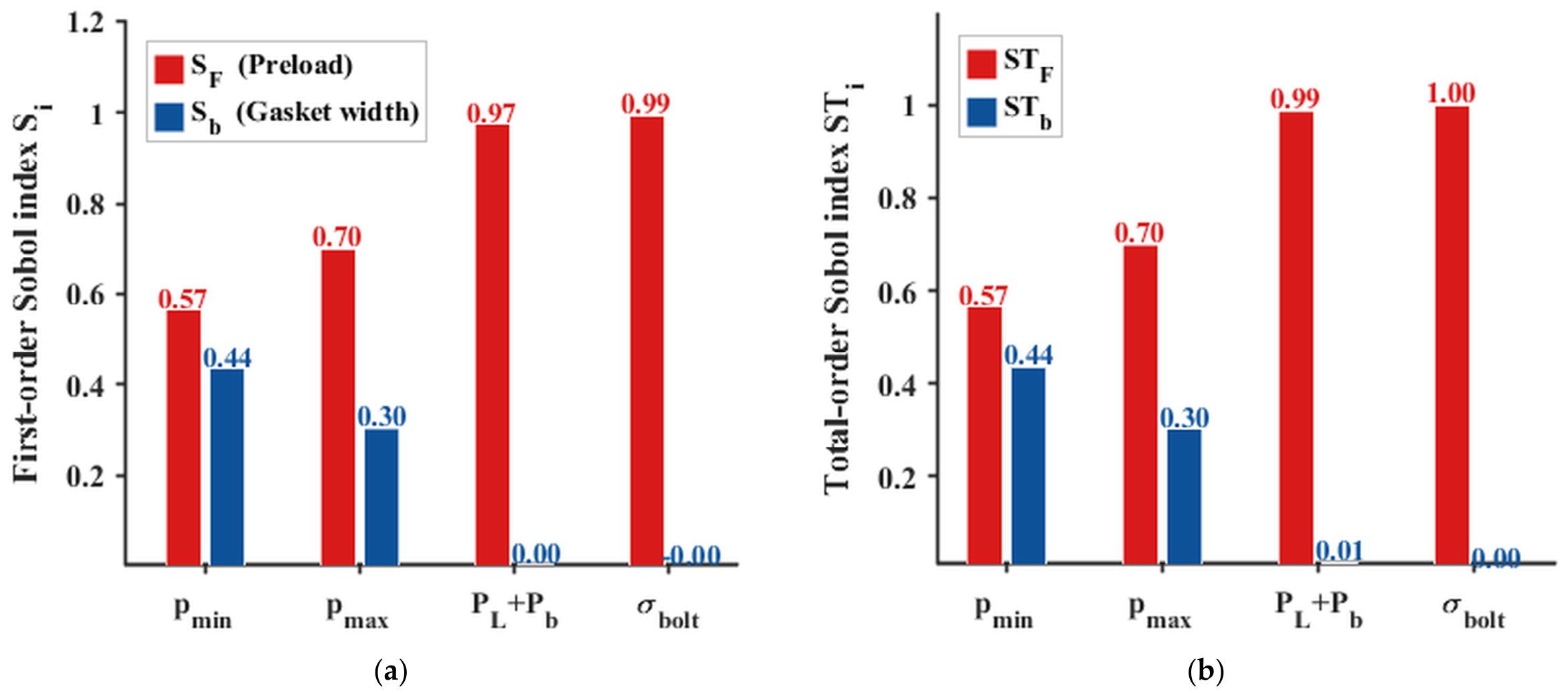
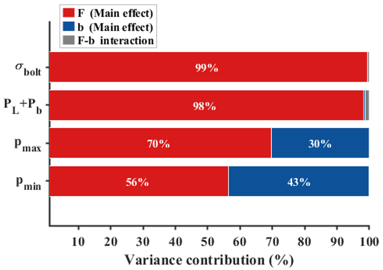
The Sobol indices for all four responses are listed in Table 19, with visualizations shown in Figure 20 and Figure 21.

As shown in Table 19, the three-term closure $S_F+S_b+S_{FB}=1$ is satisfied exactly for every response by construction, since the indices are derived analytically from the closed-form expressions in Section 4.4.1. The interaction term contribution ($S{T}_i-S_i$) does not exceed 0.86% for any response, indicating that F and b are approximately independent within the design space. Figure 20 presents the first-order main-effect and total-effect indices for all four responses as grouped bar charts; the two sets of indices are numerically very close and visually nearly indistinguishable, providing a direct graphical confirmation of approximate variable independence.

Figure 21 reveals two distinct hierarchical patterns across the four responses. In the jointly controlled pattern—$p_{min}$ (F/b ≈ 56.0%/43.1%) and $p_{max}$ (≈69.6%/29.8%)—the underlying mechanism is that increasing F compresses the gasket more uniformly, while decreasing b concentrates the contact pressure over a smaller area. In the F-dominated pattern—$P_l+P_b$ ($S_F$ = 98.8%) and ${\sigma }_{bolt}$ ($S_F$ = 100.0%)—the contribution of b is below 1.5% for both responses. The value $S_b$ = 0.0000 for ${\sigma }_{bolt}$ is essentially zero, corroborating the finding in Section 4.2.1 that all b-related RSM regression coefficients were statistically insignificant (p > 0.4). This hierarchical structure indicates that b is indispensable when $p_{min}$ is the primary objective, whereas the $P_l+P_b$ and ${\sigma }_{bolt}$ constraints can be treated approximately as single-variable constraints in F during optimization.

4.5. NSGA-II Multi-Objective Optimization

4.5.1. Pareto Front and Single-Variable Collapse

Based on the RSM surrogate model, the following multi-objective optimization problem was solved [40]:

$$max f_1\left(x\right)=p_{min}\left(x\right), \min f_2\left(x\right)=\left(P_l+P_b\right)\left(x\right)$$

(14)

$$s.t.\left\{\begin{array}{c}{p}_{max}\le 210\\ {\sigma }_{bolt}\le 580\\ p_{min}\ge 12\\ P_l+P_b\le 186\end{array}\right.$$

$$45000\le F\le 75000 \mathrm{N}, 19\le b\le 29 \mathrm{mm}$$

where $\mathbf{x}=(F,b{)}^{\mathrm{T}}$ is the design variable vector, $f_1$ and $f_2$ are evaluated through the RSM [Equation (8)], and all constraint quantities are in MPa.

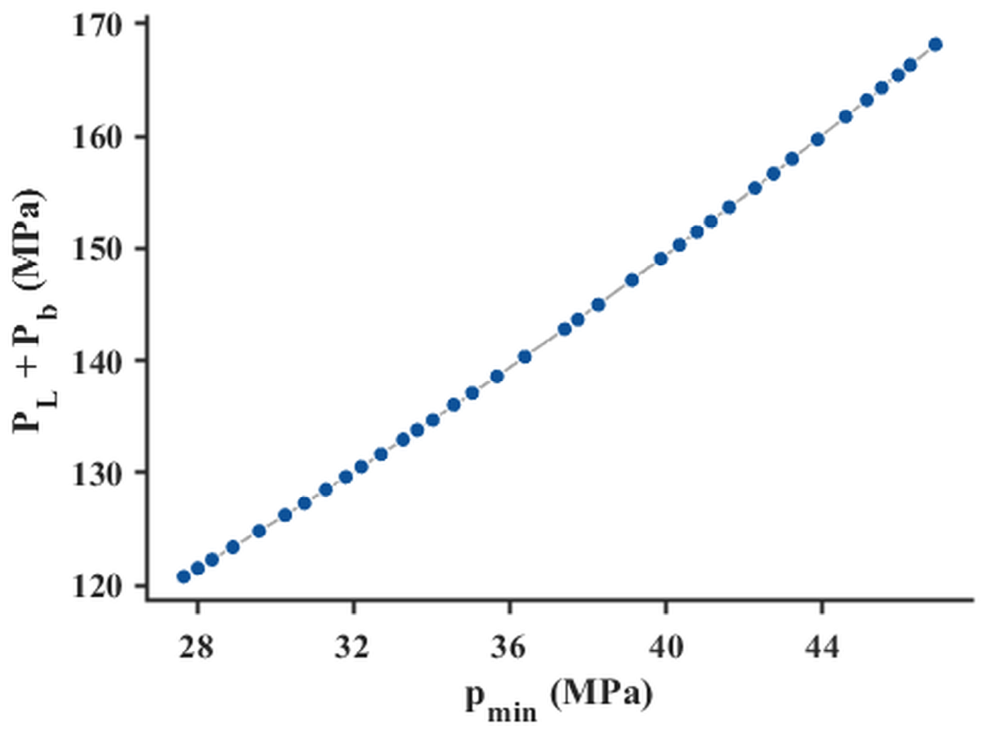
NSGA-II algorithm parameters were set as follows: population size 200, maximum generations 300, intermediate-crossover probability 0.8, mutation operator ‘mutationa-daptfeasible’ (the MATLAB default for constrained gamultiobj, which adaptively rescales mutation step sizes to preserve linear-constraint and bound feasibility), Pareto retention fraction 0.5, and function tolerance 10⁻⁶; the algorithm was implemented in MATLAB R2024a Global Optimization Toolbox. A consolidated list of the algorithm parameters used throughout this study (RSM, Kriging, Sobol analytical decomposition, NSGA-II, and TOPSIS) is provided in Supplementary Table S2, with the optimisation-pipeline pseudo-code given in Supplementary Algorithm S1. After convergence over 300 generations, 110 non-dominated solutions were obtained, forming the complete Pareto front (Figure 22).

As shown in Figure 22, the Pareto front is a smooth, continuous, and monotonically increasing near-linear curve, with endpoints at ($p_{min}$ = 27.66 MPa, $P_l+P_b$ = 120.79 MPa) and ($p_{min}$ = 46.88 MPa, $P_l+P_b$ = 168.14 MPa). The two objectives exhibit a pronounced positive correlation along the front, indicating that, within the current design space, improving the sealing contact pressure inevitably comes at the cost of increased flange stress—a genuine engineering trade-off.

Statistical analysis of the design variable distribution across the Pareto points reveals that the gasket width b collapses almost entirely to the design lower bound of 19 mm throughout the front (variation < 0.02 mm), while the pretension force F is continuously distributed over [45,000, 73,289] N. The Pareto front thus degenerates to a one-dimensional curve driven by F in the b dimension.

This phenomenon reveals the non-conflicting relationship between F and b with respect to both objectives. From the Sobol analysis in Section 4.4, b contributes only approximately 1.5% to $P_l+P_b$ (effectively zero), meaning b has virtually no influence on flange stress; the RSM regression shows that the coefficient of b for $p_{min}$ ${\beta }_b$ = −7.332 (p < 0.001), meaning smaller b yields larger $p_{min}$. Combining these two findings, the physical conclusion is that, for a fixed F, reducing b monotonically improves sealing performance without increasing structural risk—b has no genuine trade-off against either $p_{min}$ or $P_l+P_b$, and the Pareto optimum naturally converges to the lower bound of b.

The engineering implication of this finding is that the optimization of gasket width can be decoupled from the selection of pretension force: engineers can directly determine the minimum feasible value of b based on material crush strength and geometric constraints, concentrating design freedom on the trade-off selection of F and significantly simplifying the multi-parameter coordination process in engineering practice. The validity of this conclusion is premised on the design space defined in Table 13.

The bound is set jointly by the radial geometric envelope of the DN200 PN40 raised face (with the gasket constrained to sit outside the φ200 mm pipe bore and inside the bolt-circle clearance, the usable radial band is approximately 19–29 mm), by the dimensional specifications of standard spiral-wound gaskets (ASME B16.20 and manufacturers’ commercial size tables list 19 mm as the narrowest width certified for a DN200 PN40 raised-face flange), and by gasket structural integrity, since a width below ~19 mm would compromise the winding density and the outer guide ring required to retain the spiral-wound filler under high-temperature service. The collapse to $b=19 \mathrm{mm}$ therefore reflects an active engineering bound imposed by raised-face geometry, dimensional standards, and gasket manufacturability rather than a free numerical optimum; the TOPSIS-recommended design ($F=\mathrm{59,942} \mathrm{N}$, b = 19.00 mm) is best understood as the optimal pretension at the smallest commercially feasible gasket width for this flange size.

4.5.2. Constraint Activation Analysis

At the endpoint of the Pareto front (F = 73,289 N), ${\sigma }_{bolt}$ reaches 561 MPa, which still retains a 3.3% margin below the ASME II-D allowable upper limit of 580 MPa. This result indicates that the pretension upper bound $F_u$ = 75,000 N adopted in this study both captures the approaching trend of the ${\sigma }_{bolt}$ physical constraint and preserves a reasonable engineering safety margin, confirming that the design space boundaries are appropriately set. Within this design space, the path of improving sealing performance ($p_{min}$) through increasing F is effectively bounded by the allowable stress margin, consistent with the conservative principles of pressure vessel bolt design. The constraint activation diagnosis is summarized in

Table 20. Constraint activation diagnosis on the Pareto front.

Constraint	Upper Limit	Critical Value on Front	Status
${\sigma }_{bolt}$ ≤ 580 MPa	580	561.00	Not activated
$p_{max}$ ≤ 210 MPa	210	54.66	Not activated
$P_l+P_b$ ≤ 186 MPa	186	168.14	Not activated
$p_{min}$ ≥ 12 MPa	12	27.66 (min)	Not activated

.

4.6. TOPSIS Decision-Making and Weight Sensitivity Analysis

4.6.1. Equal-Weight Optimal Solution

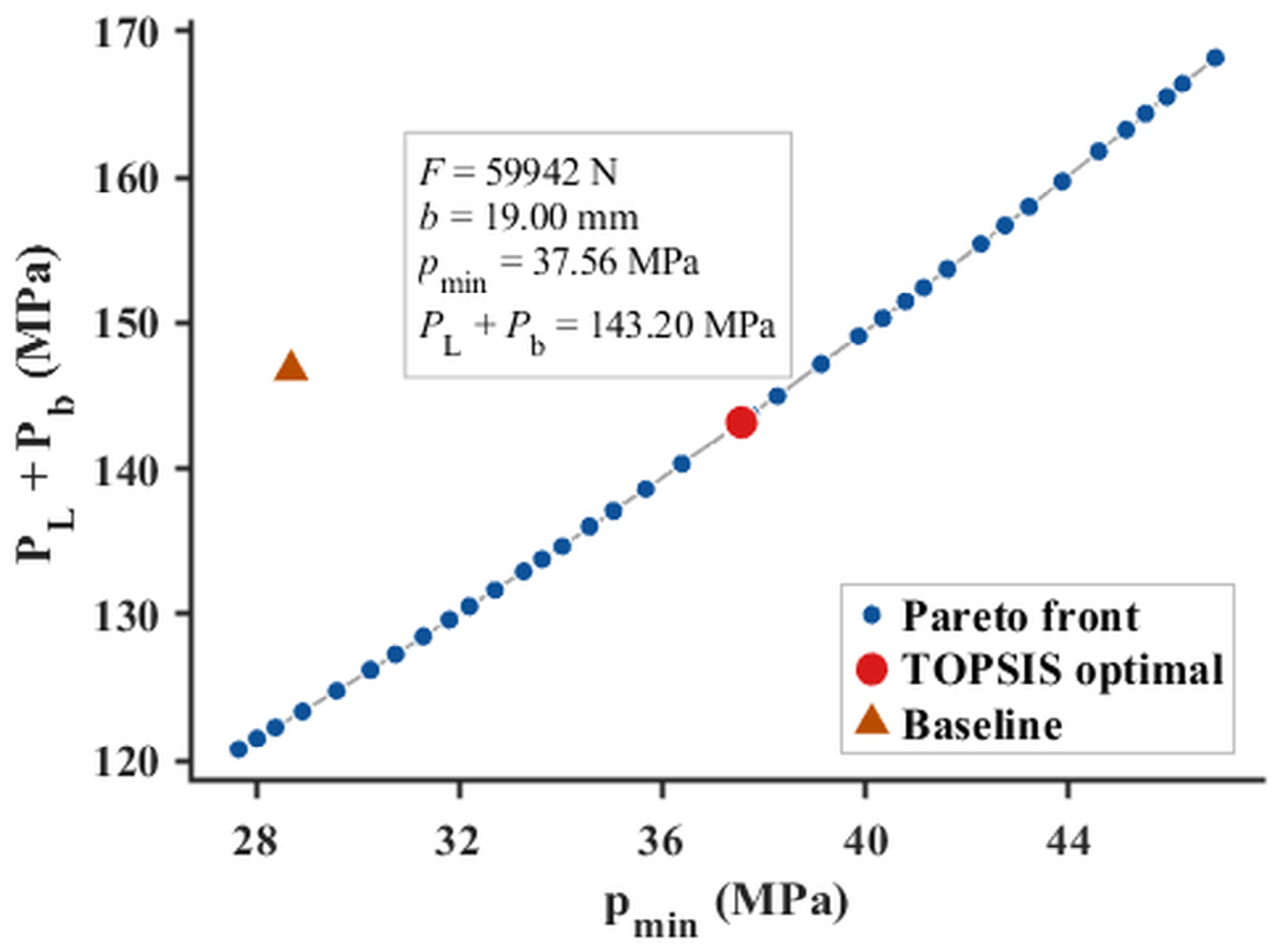
TOPSIS selects the compromise solution by means of the relative closeness coefficient C ∈ [0, 1]. Min-max normalization was applied in this study, and under equal weights, the TOPSIS method selects the optimal solution F = 59,942 N, b = 19.00 mm (C = 0.5208). The predicted responses are listed in

Table 21. TOPSIS optimal solution and top-5 candidate solutions.

Rank	F (N)	b (mm)	${\mathit{p}}_{\mathit{m}\mathit{i}\mathit{n}}$ (MPa)	${\mathit{P}}_{\mathit{l}}+{\mathit{P}}_{\mathit{b}}$ (MPa)	C
1	59,942	19.00	37.56	143.20	0.5208
2	59,726	19.01	37.41	142.83	0.5206
3	60,010	19.01	37.60	143.31	0.5205
4	59,136	19.01	37.00	141.84	0.5204
5	60,230	19.01	37.74	143.69	0.5204

, and the decision visualization is shown in Figure 23.

As shown in Table 21, the closeness coefficients C of the top-5 solutions span a range of only 0.0004, with F concentrated in [59,136, 60,230] N (range < 1.9%) and b concentrated in [19.00, 19.01] mm. This clustering behavior indicates that the equal-weight TOPSIS decision exhibits high internal consistency, and selecting F = 59,942 N, b = 19.00 mm as the recommended design parameters is well representative of the optimal region. In Figure 23, the TOPSIS optimal solution is marked by a red dot and the baseline condition by an orange triangle; the baseline lies outside the Pareto front, confirming the necessity of optimization.

Relative to the baseline condition (F = 60,000 N, b = 24 mm), the optimal solution achieves: $p_{\mathrm{m}\mathrm{i}\mathrm{n}}$ + 30.87%, $P_l+P_b$ − 2.43%, and ${\sigma }_{bolt}$ virtually unchanged (+0.75 MPa). All percentages quoted in this paragraph are RSM-predicted improvements relative to the baseline; the corresponding ANSYS back-substitution verified improvements (+31.01% in $p_{min}$ and −2.26% in $P_l+P_b$) are reported in Section 4.7 and

Table 22. ANSYS back-substitution verification results.

Response	Baseline	RSM Prediction	ANSYS Verification	Improvement vs. Baseline	Prediction Error
$p_{min}$ (MPa)	28.70	37.56	37.60	+31.01%	+0.11%
$p_{max}$ (MPa)	35.51	43.94	44.11	+24.22%	+0.40%
$P_l+P_b$ (MPa)	146.76	143.20	143.45	−2.26%	+0.17%
${\sigma }_{bolt}$ (MPa)	476.98	477.73	471.98	−1.05%	−1.22%

, with a prediction error of +0.11% on $p_{min}$.

4.6.2. Weight Sensitivity Analysis

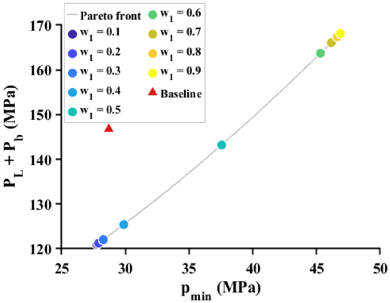
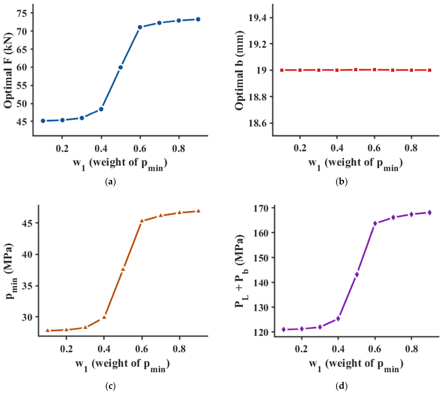
Nine weight combinations were scanned over w₁ ∈ [0.1, 0.9] in steps of 0.1 (with $w_2=1-w_1$); results are presented in Figure 24 and Figure 25. Along the F dimension, the Pareto front exhibits a three-stage transition: conservative design ($w_1$ ∈ [0.1, 0.4], $F\approx \mathrm{45,000}-\mathrm{48,000} \mathrm{N}$), balanced design ($w_1$ = 0.5, $F=\mathrm{59,942} \mathrm{N}$, the equal-weight optimum), and aggressive design ($w_1$ ∈ [0.6, 0.9], $F\approx \mathrm{71,000}-\mathrm{73,000} \mathrm{N}$)—providing quantitative guidance for engineers to select parameters according to service conditions.

As shown in Figure 24, the TOPSIS optimal solutions under the nine weight combinations cluster into three groups on the Pareto front: the four solutions with w₁ ∈ [0.1, 0.4] concentrate at the lower-left end of the front ($p_{min}$ ≈ 28 MPa, $P_l+P_b$≈ 121 MPa), the four solutions with w₁ ∈ [0.6, 0.9] concentrate at the upper-right end ($p_{min}$ ≈ 46 MPa, $P_l+P_b$ ≈ 166 MPa), and only the equal-weight solution at w₁ = 0.5 falls in the middle segment of the front ($p_{min}$ = 37.56 MPa, $P_l+P_b$ = 143.20 MPa). Figure 25 further shows that F, $p_{min}$, and $P_l+P_b$ all vary as S-shaped step curves with respect to w₁, with the transition concentrated in the interval w₁ ∈ [0.4, 0.6], while b remains stable at 19.00 mm throughout the entire scan (variation < 0.002 mm). The root cause of this behavior is that the near-linear structure of the Pareto front causes the TOPSIS closeness function to attain local maxima at both ends of the front, so that small perturbations in weight can switch the optimal index between the two end clusters—an intrinsic characteristic of applying TOPSIS to a linear front. Taken together, the two figures indicate that the cross-weight robustness of b = 19.00 mm identifies the gasket width lower bound as the global optimum for this problem, while F = 59,942 N, as the inflection point of the S-shaped transition curve, represents the critical balance between sealing performance preference and flange stress preference, and constitutes the engineering-rational recommendation under equal-weight decision-making.

4.7. ANSYS Back-Substitution Verification

The TOPSIS-recommended solution (F = 59,942 N, b = 19.00 mm) was substituted into the ANSYS Workbench finite element model established in Section 3. The geometric modification followed the strategy of a fixed outer diameter with adjusted inner diameter, consistent with the CCD experimental design. The simulation was solved sequentially in three steps—bolt pretensioning, internal pressure and equivalent tensile stress loading, and 300 °C steady-state temperature field import—and the four core responses were extracted and compared against the RSM predictions and the baseline condition. Results are listed in Table 22.

As shown in Table 22, the relative errors of all four core responses are within 1.22%, well below the 5% acceptance threshold, confirming that the RSM surrogate model possesses engineering-level predictive reliability at the TOPSIS-recommended solution. The slightly larger error for ${\sigma }_{bolt}$ arises because the weak second-order nonlinearity of this response in the b dimension is not fully captured by the second-order polynomial, which is consistent with the low-order noise characteristics of ${\sigma }_{bolt}$ with respect to b identified in the Sobol analysis of Section 4.4.

Based on the ANSYS-verified values, the optimized solution achieves coordinated improvement in both sealing performance and structural integrity relative to the baseline: $p_{min}$ increases from 28.70 MPa to 37.60 MPa (+31.01%), $P_l+P_b$ decreases from 146.76 MPa to 143.45 MPa (−2.26%), and ${\sigma }_{bolt}$ decreases from 476.98 MPa to 471.98 MPa (−1.05%), retaining a safety margin of 108 MPa below the ASME II-D allowable upper limit of 580 MPa. The core improvement pathway is as follows: with F held approximately constant (≈ 60,000 N), reducing b from 24 mm to the lower bound of 19 mm increases the contact pressure per unit area, substantially raising $p_{min}$, while the shortened bending moment arm reduces $P_l+P_b$. This result quantitatively corroborates the prediction from the Sobol analysis in Section 4.4, validating the engineering conclusion that “b = 19 mm is the robust global optimum within the design space”.

5. Conclusions

This study developed a steady-state thermal–structural sequential coupling finite element model in ANSYS Workbench to investigate the sealing reliability of a DN200 PN40 weld-neck flange–bolt–gasket system under 300 °C high-temperature superheated steam conditions. Through response surface surrogate modeling, Sobol global sensitivity analysis, and NSGA-II multi-objective optimization, the coupled effects of bolt pretension F and gasket width b on sealing performance and structural integrity were systematically examined. The principal conclusions are as follows:

• The 1/12 periodic sector thermal–structural sequential coupling finite element model was validated against the Omiya–Sawa 3-inch WN flange benchmark at two levels—Level 1: bolt load against experimental measurements; Level 2: high-temperature gasket contact pressure distribution against the reference finite-element results—with maximum relative errors below 1.5% in both cases, establishing the reliability of the modeling procedure for the DN200 PN40 configuration rather than constituting a direct experimental validation thereof. Baseline analysis based on this model revealed the “inner-loose, outer-tight” failure mechanism of high-temperature flange sealing systems: under the combined action of bolt pretension and internal pressure, the flange body undergoes bending deformation about the hub fillet, producing a flange rotation of −0.308°. This causes the gasket contact pressure to distribute monotonically along the radial direction, with a lower value at the inner radius (28.70 MPa) and a higher value at the outer radius (35.50 MPa). The minimum contact pressure $p_{min}$ occurs at the inner radius and represents the critical sealing failure path, providing direct physical justification for adopting $p_{min}$ as the primary optimization objective.
• The second-order response surface model achieved MAPEs of 0.72%, 0.84%, 0.97%, and 1.90% on the independent validation set for $p_{min}$, $p_{max}$, $P_l+P_b$, and ${\sigma }_{bolt}$, respectively—approximately five times more accurate than the Kriging model for the primary objective $p_{min}$ under the same sample size, demonstrating that RSM is more suitable than Kriging for the specific multi-response sealing problem considered in this study, involving small sample sizes and smooth second-order response surfaces. Sobol global sensitivity analysis further revealed that F and b are approximately independent within the design space (interaction contributions below 1.5%), and that the four responses exhibit two distinct dominance patterns: $p_{min}$ and $p_{max}$ are jointly controlled by both F and b, whereas $P_l+P_b$ and ${\sigma }_{bolt}$ are overwhelmingly dominated by F alone (contribution rates exceeding 97%). This hierarchical structure provides a quantitative justification for decoupled variable treatment in the subsequent optimization.
• The Pareto front obtained by NSGA-II collapsed to the design lower bound b = 19 mm in the gasket width dimension, revealing the non-conflicting nature of F and b with respect to both objectives: at fixed F, reducing b monotonically improves sealing performance without increasing the structural risk to the flange, enabling the selection of gasket width and bolt pretension to be treated independently in engineering design. TOPSIS with equal weights recommended F = 59,942 N and b = 19.00 mm as the optimal compromise solution. ANSYS back-substitution verification showed that this solution increased $p_{min}$ from 28.70 MPa to 37.60 MPa (+31.01%), reduced $P_l+P_b$ from 146.76 MPa to 143.45 MPa (−2.26%), and decreased ${\sigma }_{bolt}$ from 476.98 MPa to 471.98 MPa (−1.05%), retaining a safety margin of 108 MPa below the ASME II-D allowable limit of 580 MPa—achieving coordinated improvement in both sealing performance and structural safety.

The engineering value of this study lies in providing quantitative decision-making guidance for the selection of design parameters in high-temperature flange–bolt–gasket systems. The integrated framework of surrogate modeling–sensitivity analysis–multi-objective optimization–back-substitution verification established here is methodologically transferable to sealing performance optimization of flange assemblies in other specifications; the specific quantitative improvements reported above (+31.01% in $p_{min}$ and −2.26% in $P_l+P_b$), however, are tied to the analysed DN200 PN40 configuration, the spiral-wound gasket type, the A105/A193 B7 temperature-dependent material set, and the steady-state 300 °C/4 MPa superheated-steam service condition, and should not be extrapolated to other flange sizes, gasket types, or service media without further parametric analysis. Future work may extend in five directions: first, incorporating additional geometric variables such as gasket thickness and hub height into a multi-variable co-optimization to re-examine variable coupling relationships within a broader design space; second, moderately expanding the upper bound of bolt pretension to further exploit the potential for sealing performance improvement while preserving adequate engineering safety margins; and third, introducing gasket creep and bolt stress relaxation constitutive models to conduct transient thermal–structural coupling analyses, thereby characterizing the long-term sealing reliability evolution under start-up and shutdown cycling conditions; fourth, replacing the $m·P$ sealing screening criterion adopted here with a leakage-rate-based qualification such as the PVRC tightness-class methodology [43] or the Jaszak leakage correlations [4,32], so that the absolute admissible level of $p_{min}$ is calibrated directly against measurable leakage classes; and fifth, incorporating experimentally measured spiral-wound-gasket unloading curves and temperature-dependent thermal conductivity into the INTER194 element data, so that the Step-2 spring-back and Step-3 redistribution responses can be modelled with the full hysteretic constitutive behaviour rather than the conservative linear unloading idealisation used in this work.

References

1. Nelson, N.R.; Prasad, N.S.; Sekhar, A.S. Structural Integrity and Sealing Behaviour of Bolted Flange Joint: A State of Art Review. Int. J. Press. Vessels Pip. 2023, 204, 104975. [Google Scholar] [CrossRef]
2. Cloostermans, B.; Pronk, D.; Bruckenburg, B.; Goossens, S.; Baghdasaryan, T.; Berghmans, F. Bolted Flange Connection Leakage: A Systematic Review of Monitoring Challenges and Technologies. IEEE Sens. Rev. 2025, 2, 1–16. [Google Scholar] [CrossRef]
3. Marek, P.; Pawlicki, J.; Mościcki, A. Tightness Problems at the Flange Connection in Transient Temperature and High Pressure Condition. Eng. Fail. Anal. 2022, 133, 105986. [Google Scholar] [CrossRef]
4. Jaszak, P.; Grzejda, R. Symmetric and Asymmetric Semi-Metallic Gasket Cores and Their Effect on the Tightness Level of the Bolted Flange Joint. Materials 2025, 18, 2624. [Google Scholar] [CrossRef] [PubMed]
5. Jaszak, P.; Grzejda, R.; Kluczyński, J.; Zmarzły, P. Basic Design Parameters Influencing on Axial Stiffness of the Spiral Wound Gasket. Materials 2023, 16, 6209. [Google Scholar] [CrossRef] [PubMed]
6. Jaszak, P.; Piwowar, A.; Bieganowski, M. Influence of Sealing Surface Microstructure Characteristics on Flow Resistance and Leakage Between Contact Surfaces. Materials 2025, 18, 4474. [Google Scholar] [CrossRef] [PubMed]
7. Sawa, T.; Kobayashi, T.; Tsuji, H.; Nagata, S. Stress Analysis and a Design Method for Bolted Pipe Flanged Joints Subjected to Internal Pressure. In Proceedings of the Volume 2: Computer Applications/Technology and Bolted Joints, Prague, Czech Republic, 26–30 July 2009; ASMEDC: Prague, Czech Republic, 2009; pp. 157–167. [Google Scholar]
8. Takagi, Y.; Torii, H.; Sawa, T.; Omiya, Y. Sealing Performance Evaluation of Pipe Flange Connection with Spiral Wound Gasket Under Cyclic Thermal Condition. In Proceedings of the Volume 2: Computer Applications/Technology and Bolted Joints, Prague, Czech Republic, 26–30 July 2009; ASMEDC: Prague, Czech Republic, 2009; pp. 131–137. [Google Scholar]
9. Fukuoka, T.; Nomura, M.; Nishikawa, T. Analysis of Thermal and Mechanical Behavior of Pipe Flange Connections by Taking Account of Gasket Compression Characteristics at Elevated Temperature. J. Press. Vessel Technol. 2012, 134, 021202. [Google Scholar] [CrossRef]
10. Bouzid, A.-H.; Nechache, A. An Analytical Solution for Evaluating Gasket Stress Change in Bolted Flange Connections Subjected to High Temperature Loading. J. Press. Vessel Technol. 2005, 127, 414–422. [Google Scholar] [CrossRef]
11. Nechache, A.; Bouzid, A.-H. Creep Analysis of Bolted Flange Joints. Int. J. Press. Vessels Pip. 2007, 84, 185–194. [Google Scholar] [CrossRef]
12. Abid, M. Determination of Safe Operating Conditions for Gasketed Flange Joint under Combined Internal Pressure and Temperature: A Finite Element Approach. Int. J. Press. Vessels Pip. 2006, 83, 433–441. [Google Scholar] [CrossRef]
13. Bian, D.; Sun, Y.; Wei, Z.; Chen, C.; Zhou, J.; Shao, C. Time-Dependent Leakage Rate Prediction Method for Bolted Flange Connection Based on Equivalent Stress-Temperature. Proc. Inst. Mech. Eng. Part E J. Process Mech. Eng. 2024, 240, 09544089241282819. [Google Scholar] [CrossRef]
14. Aljuboury, M.; Rizvi, M.J.; Grove, S.; Cullen, R. A Numerical Investigation of the Sealing Performance and the Strength of a Raised Face Metallic Bolted Flange Joint. Int. J. Press. Vessels Pip. 2021, 189, 104255. [Google Scholar] [CrossRef]
15. Murali Krishna, M.; Shunmugam, M.S.; Siva Prasad, N. A Study on the Sealing Performance of Bolted Flange Joints with Gaskets Using Finite Element Analysis. Int. J. Press. Vessels Pip. 2007, 84, 349–357. [Google Scholar] [CrossRef]
16. Mathan, G.; Siva Prasad, N. Studies on Gasketed Flange Joints under Bending with Anisotropic Hill Plasticity Model for Gasket. Int. J. Press. Vessels Pip. 2011, 88, 495–500. [Google Scholar] [CrossRef]
17. Liu, D.; Yun, F.; Wang, W.; Jiao, K.; Wang, L.; Yan, Z.; Jia, P.; Wang, X.; Liu, W.; Sun, H.; et al. Sealing Contact Transient Thermal-Structural Coupling Analysis of the Subsea Connector. Machines 2022, 10, 213. [Google Scholar] [CrossRef]
18. Yun, F.; Liu, D.; Xu, X.; Jiao, K.; Hao, X.; Wang, L.; Yan, Z.; Jia, P.; Wang, X.; Liang, B. Thermal–Structural Coupling Analysis of Subsea Connector Sealing Contact. Appl. Sci. 2022, 12, 3194. [Google Scholar] [CrossRef]
19. He, L.; Zhong, F. Multi-Objective Co-Optimization of Operation and Geometry for Liquid-Cooled Heat Sinks Using an Integrated CFD–RSM–NSGA-II Framework. AIP Adv. 2025, 15, 115326. [Google Scholar] [CrossRef]
20. Wen, P.; Wang, S.; Li, J.; Dong, K.; Ren, Z.; Li, Y.; Qu, R.; Li, T. Multiobjective Optimization of a Pressure Maintaining Ball Valve Structure Based on RSM and NSGA-II. Sci. Rep. 2025, 15, 21342. [Google Scholar] [CrossRef] [PubMed]
21. He, Y.; Lu, D.; Li, Z.; Lu, D. Multi-Objective Optimization of The Low-Pressure Casting of Large-Size Aluminum Alloy Wheels through a Systematic Optimization Idea. Materials 2023, 16, 6223. [Google Scholar] [CrossRef] [PubMed]
22. Deb, K.; Pratap, A.; Agarwal, S.; Meyarivan, T. A Fast and Elitist Multiobjective Genetic Algorithm: NSGA-II. IEEE Trans. Evol. Comput. 2002, 6, 182–197. [Google Scholar] [CrossRef]
23. Ma, H.; Zhang, Y.; Sun, S.; Liu, T.; Shan, Y. A Comprehensive Survey on NSGA-II for Multi-Objective Optimization and Applications. Artif. Intell. Rev. 2023, 56, 15217–15270. [Google Scholar] [CrossRef]
24. Saltelli, A.; Annoni, P.; Azzini, I.; Campolongo, F.; Ratto, M.; Tarantola, S. Variance Based Sensitivity Analysis of Model Output. Design and Estimator for the Total Sensitivity Index. Comput. Phys. Commun. 2010, 181, 259–270. [Google Scholar] [CrossRef]
25. Shang, X.; Su, L.; Fang, H.; Zeng, B.; Zhang, Z. An Efficient Multi-Fidelity Kriging Surrogate Model-Based Method for Global Sensitivity Analysis. Reliab. Eng. Syst. Saf. 2023, 229, 108858. [Google Scholar] [CrossRef]
26. Zhu, L.; Qiu, J.; Chen, M.; Jia, M. Approach for the Structural Reliability Analysis by the Modified Sensitivity Model Based on Response Surface Function—Kriging Model. Heliyon 2022, 8, e10046. [Google Scholar] [CrossRef] [PubMed]
27. Hwang, C.-L.; Yoon, K. Multiple Attribute Decision Making: Methods and Applications, A State-of-the-Art Survey; Springer: Berlin/Heidelberg, Germany, 1981. [Google Scholar]
28. Madanchian, M.; Taherdoost, H. A Comprehensive Guide to the TOPSIS Method for Multi-Criteria Decision Making. Sustain. Social. Dev. 2023, 1, 2220. [Google Scholar] [CrossRef]
29. Wang, J.; Zhu, J.; Hou, J.; Wang, C.; Zhang, W. Lightweight Design of a Bolt-Flange Sealing Structure Based on Topology Optimization. Struct. Multidisc Optim. 2020, 62, 3413–3428. [Google Scholar] [CrossRef]
30. Wang, K.; Liu, J.; Gong, H.; Deng, X. Robust Optimization Design for Sealing Performance of Globe-Cone Joint Considering Manufacturing and Assembly Uncertainties. Struct. Multidisc Optim. 2023, 66, 92. [Google Scholar] [CrossRef]
31. Zacal, J.; Folta, Z.; Struz, J.; Trochta, M. Influence of Symmetry of Tightened Parts on the Force in a Bolted Joint. Symmetry 2023, 15, 276. [Google Scholar] [CrossRef]
32. Jaszak, P.; Skrzypacz, J.; Borawski, A.; Grzejda, R. Methodology of Leakage Prediction in Gasketed Flange Joints at Pipeline Deformations. Materials 2022, 15, 4354. [Google Scholar] [CrossRef] [PubMed]
33. ASME. PCC-1-Pressure Boundary Bolted Flange Joint Assembly; ASME: New York, NY, USA, 2022. [Google Scholar]
34. ASTM A105/A105M-26; Standard Specification for Carbon Steel Forgings for Piping Applications. ASTM International: West Conshohocken, PA, USA, 2026.
35. ASTM A193/A193M-26; Standard Specification for Alloy-Steel and Stainless Steel Bolting for High Temperature or High Pressure Service and Other Special Purpose Applications. ASTM International: West Conshohocken, PA, USA, 2026.
36. Waleed, M.; Lee, D. Investigation of Bolt Grade Influence on the Structural Integrity of L-Type Flange Joints Using Finite Element Analysis. J. Mar. Sci. Eng. 2025, 13, 1346. [Google Scholar] [CrossRef]
37. Zhang, Y.; Jiao, P.; Du, W.; Qi, G.; Chen, B. Numerical Simulation of Casting Filling Process Based on SPH-FEM Coupling Method. Symmetry 2025, 17, 494. [Google Scholar] [CrossRef]
38. Qi, G.; Jiao, P.; Du, W.; Zhang, Y.; Chen, B. Simulation and Optimization of Train Brake Disc Based on Coupling Characteristics of FEM and Thermal Flow Density Method. Sci. Rep. 2025, 15, 40617. [Google Scholar] [CrossRef] [PubMed]
39. Bickford, J.H.; Oliver, M. Introduction to the Design and Behavior of Bolted Joints: Non-Gasketed Joints, 5th ed.; CRC Press: Boca Raton, FL, USA, 2022. [Google Scholar]
40. Croccolo, D.; De Agostinis, M.; Fini, S.; Khan, M.Y.; Mele, M.; Olmi, G. Optimization of Bolted Joints: A Literature Review. Metals 2023, 13, 1708. [Google Scholar] [CrossRef]
41. He, B.; Jiao, B.; Wan, Q.; Nie, R.; Yang, J. Strength and Tightness Evaluation Method for Pipe Flange Connections Considering Thermal Effects. J. Loss Prev. Process Ind. 2023, 83, 105053. [Google Scholar] [CrossRef]
42. Raghavaiah, N. Overview of Pressure Vessel Design Using ASME Boiler and Pressure Vessel Code Section VIII Division-1 and Division-2. Int. J. Res. Eng. Sci. Manag. 2019, 2, 525–526. [Google Scholar]
43. Payne, J.R.; Bazergui, A.; Leon, G.F. New Gasket Factors—A Proposed Procedure. In Proceedings of the Proceedings of the ASME Pressure Vessel and Piping Conference, New Orleans, LA, USA, 24–29 June 1985; American Society of Mechanical Engineers: Pittsburgh, PA, USA, 1985; Volume PVP-Vol. 98-2, pp. 85–93. [Google Scholar]
44. ISO 898-1:2013; Mechanical Properties of Fasteners Made of Carbon Steel and Alloy Steel—Part 1: Bolts, Screws and Studs with Specified Property Classes—Coarse Thread and Fine Pitch Thread. International Organization for Standardization: Geneva, Switzerland, 2013.
45. Mir-Haidari, S.-E.; Behdinan, K. Nonlinear Effects of Bolted Flange Connections in Aeroengine Casing Assemblies. Mech. Syst. Signal Process. 2022, 166, 108433. [Google Scholar] [CrossRef]
46. Liu, X.; Bu, Q.; Luan, S.; Cao, X.; Zhang, Y.; Mu, C.; Lin, J.; Shi, Y. Analysis of Sealing Characteristics of Hydraulic Clamping Flange Connection Mechanism. Processes 2026, 14, 72. [Google Scholar] [CrossRef]
47. Mackenzie, D. Stress Linearization Concepts and Restrictions in Elastic Design by Analysis. In Proceedings of the Volume 1A: Codes and Standards; American Society of Mechanical Engineers: Waikoloa, HI, USA, 2017; p. V01AT01A039. [Google Scholar]
48. Hechmer, J.; Hollinger, G.L. 3D Stress Criteria Guidelines for Application; WRC BULLETIN; WRC: Shaker Heights, OH, USA, 1998. [Google Scholar]
49. Rasmussen, C.E.; Williams, C.K.I. Gaussian Processes for Machine Learning; The MIT Press: Cambridge, MA, USA, 2005. [Google Scholar]
Figure 1. Three-dimensional assembly model of the flange–bolt–gasket system.
Symmetry 18 01252 g001
Figure 2. Annotated geometry of the flange–bolt–gasket system (unit: mm).
Symmetry 18 01252 g002
Figure 3. 1/12 periodic sector finite element geometry model.
Symmetry 18 01252 g003
Figure 4. Finite element mesh of the 1/12 sector.
Symmetry 18 01252 g004
Figure 5. Schematic of the boundary conditions for the 1/12 model.
Symmetry 18 01252 g005
Figure 6. Comparison of bolt load F f + F t versus internal pressure P (3-inch flange, ambient temperature).
Symmetry 18 01252 g006
Figure 7. Comparison of radial gasket contact pressure distribution at 250 °C.
Symmetry 18 01252 g007
Figure 8. Steady-state temperature field distribution of the flange–bolt system.
Symmetry 18 01252 g008
Figure 9. Evolution of gasket contact pressure distribution across the three loading steps, plotted under a common color scale of 28–41 MPa: (a) Step 1, bolt pretensioning; (b) Step 2, internal pressure application; (c) Step 3, high-temperature operation. In each panel, the left edge corresponds to the gasket inner radius (ri = 115 mm) and the right edge to the outer radius (ro = 139 mm); the radial direction is indicated by the arrow below the panels.
Symmetry 18 01252 g009
Figure 10. Radial distribution curves of gasket contact pressure and temperature. The solid red curve denotes contact pressure; the blue dash-dotted curve denotes temperature; and the vertical gray dashed line separates the high-pressure inner side from the low-pressure outer side.
Symmetry 18 01252 g010
Figure 11. Von Mises equivalent stress distribution of the flange (Step 3, 300 °C condition). The circular opening is a bolt hole, and the local red region around it denotes a peak-stress concentration.
Symmetry 18 01252 g011
Figure 12. Membrane and bending stress distribution along the flange SCL path (based on Step 3 stress linearization results). The solid blue, dashed purple, solid red, and dotted brown curves represent membrane stress, bending stress, membrane-plus-bending stress, and the ASME allowable SPL, respectively; the vertical gray dashed line denotes the zero-bending plane.
Symmetry 18 01252 g012
Figure 13. Second-order RSM fitted surfaces: (a) p m i n ; (b) p m a x ; (c) P l + P b ; (d) σ b o l t .
Symmetry 18 01252 g013
Figure 14. RSM predicted vs. simulated values: (a) p m i n ; (b) p m a x ; (c) P l + P b ; (d) σ b o l t .
Symmetry 18 01252 g014
Figure 15. RSM standardized residual diagnostic plots: (a) p m i n ; (b) p m a x ; (c) P l + P b ; (d) σ b o l t .
Symmetry 18 01252 g015
Figure 16. Kriging fitted surfaces: (a) p m i n ; (b) p m a x ; (c) P l + P b ; (d) σ b o l t .
Symmetry 18 01252 g016aSymmetry 18 01252 g016b
Figure 17. Kriging predicted vs. simulated values: (a) p m i n ; (b) p m a x ; (c) P l + P b ; (d) σ b o l t . The dashed line denotes the ideal agreement line (y = x).
Symmetry 18 01252 g017
Figure 18. Kriging standardized residual diagnostic plots: (a) p m i n ; (b) p m a x ; (c) P l + P b ; (d) σ b o l t .
Symmetry 18 01252 g018
Figure 19. Bar chart comparison of RSM and Kriging validation-set MAPE.
Symmetry 18 01252 g019
Figure 20. Sobol sensitivity indices: (a) first-order main effects; (b) total effects.
Symmetry 18 01252 g020
Figure 21. Variance contribution decomposition for each response.
Symmetry 18 01252 g021
Figure 22. Pareto front obtained by NSGA-II.
Symmetry 18 01252 g022
Figure 23. TOPSIS decision results (min-max normalization, equal weights).
Symmetry 18 01252 g023
Figure 24. Distribution of TOPSIS optimal solutions on the Pareto front under 9 weight combinations. The light-gray line denotes the Pareto front; colored circles represent the TOPSIS solutions for w1 = 0.1–0.9, progressing from purple to yellow as w1 increases; and the red triangle denotes the baseline condition.
Symmetry 18 01252 g024
Figure 25. Optimal design variables and responses as functions of weight w1: (a) optimal preload F; (b) optimal gasket width b; (c) p m i n ; (d) P l + P b .
Symmetry 18 01252 g025