Research on Stochastic Bifurcation and Reliability of a Photovoltaic Power System Under Combined Additive and Multiplicative Random Excitation

Abstract

The random impact of photovoltaic grid connection on the system has always attracted the attention of the academic community. Therefore, using some theories of stochastic differential equations, especially the stochastic averaging method, to study the bifurcation phenomena caused by random photovoltaic output has become a growing trend. This paper models a two-machine power system excited by stochastic photovoltaic output, based on a quasi-non-integrable Hamiltonian physical model, and analyzes its dynamic behavior from two aspects: stochastic bifurcation and stochastic reliability. First, the two-machine power system is transformed into a quasi-non-integrable Hamiltonian model, through which the system equations are simplified for the following calculations. In the subsequent stochastic bifurcation analysis, we study the effects of damping coefficient and noise intensity on the bifurcation evolution. We find that combined parameter and external excitations lead to more variable bifurcation evolution scenarios. Finally, through stochastic reliability analysis, the stochastic reliability analysis demonstrates the importance of mixed parameter adjustment in maintaining the system’s reliability level. Research shows that the stochastic bifurcation caused by photovoltaic grid connection can occur within a certain range of parameters, and we believe this phenomenon provides valuable insights for subsequent studies.

1. Introduction

Photovoltaic (PV) power generation has emerged as a pivotal component in new energy grid integration owing to its clean and sustainable attributes. However, the operational stability of power systems is increasingly challenged by the significant randomness inherent in PV output, which stems from environmental weather conditions such as fluctuations in both solar irradiance and air temperature [1,2]. Unlike conventional synchronous generators, PV systems introduce stochastic power fluctuations that propagate through the grid, potentially triggering nonlinear dynamic phenomena. Consequently, analyzing the impact of stochastic PV excitation on power system dynamics is of paramount importance for ensuring grid security.

Current research methodologies addressing PV integration can be broadly categorized into static and dynamic analyses. Static analyses typically treat PV output as a deterministic or statistically averaged power source within steady-state models [3,4,5,6]. While computationally efficient, these methods often overlook the transient dynamic characteristics induced by stochastic fluctuations. Conversely, dynamic analyses model PV output as stochastic processes, employing stochastic differential equations (SDEs) to capture temporal uncertainties [7]. This is also a commonly adopted dynamic analysis method in various engineering disciplines in the literature [8,9,10,11]. However, dynamic analysis of large-scale PV grid integration remains challenging. High-dimensional differential equation systems make numerical simulation difficult [12,13]. Thus, analytical stochastic differential equation (SDE) methods are gaining attention. For instance, ref. [14] determines stability using mean and mean-square statistics. This approach, known as mean-square analysis, is applied in [15,16,17]. Alternatively, SDE analysis can integrate neural networks. Sun et al. [18] used this to calculate higher-order statistical moments, outperforming traditional methods. Similarly, ref. [19] simulated PV and wind outputs using generative technology. Among these, stochastic averaging is effective for analyzing stability, bifurcation, and reliability. It reduces system dimension by identifying slow variables via time averaging. For example, ref. [20] applied it to fractional-order systems, while ref. [21] analyzed hysteresis in energy harvesting. These traditional methods use generalized harmonic transformation [22], known as the amplitude-envelope stochastic averaging method [23,24,25].

Despite these successful applications, several critical gaps remain in the existing literature. Traditional amplitude-envelope stochastic averaging relies on generalized harmonic transformations, which may falter for strongly nonlinear systems where system frequency varies with amplitude. Meanwhile, there is a lack of studies applying the quasi-non-integrable Hamiltonian framework to PV-grid coupled systems to better capture their intrinsic physical properties. Most studies focus on static reliability or simple stability indices. The mechanisms of stochastic bifurcation—particularly P-bifurcation—under combined additive (external) and multiplicative (parametric) excitations in PV systems remain underexplored.

To bridge the aforementioned gaps, this paper proposes a comprehensive stochastic dynamic framework for a two-machine PV system. The specific contributions are summarized as follows:

(i)

Novel Modeling Approach: We establish a quasi-non-integrable Hamiltonian model for the two-machine system. By utilizing the Hamiltonian stochastic averaging method [26,27], we provide a more physically consistent representation of the system’s energy distribution under stochastic excitation.

(ii)

Mechanism of Stochastic Bifurcation: We reveal the distinct bifurcation evolution scenarios under combined additive and multiplicative excitations. We distinguish the individual and joint effects of damping coefficients and external noise intensity on the transition of probability density functions, explaining the “imperfect bifurcation” characteristics observed in PV systems.

(iii)

Multi-Parameter Reliability Regulation: We derive analytical solutions for the system’s reliability based on the backward Fokker–Planck–Kolmogorov (FPK) equation. We demonstrate that multi-parameter regulation outperforms single-parameter control in maintaining system reliability within the bounded fluctuation domain.

The remainder of this paper is structured as follows. Section 2 establishes the stochastic dynamic model of the two-machine PV system and approximates it into a quasi-non-integrable Hamiltonian form. Section 3 applies the stochastic averaging method to reduce the system to a one-dimensional diffusion process. Section 4 conducts a detailed analysis of stochastic bifurcation characteristics under varying parameters. Section 5 evaluates the system’s stochastic reliability and discusses the effects of multi-parameter regulation. 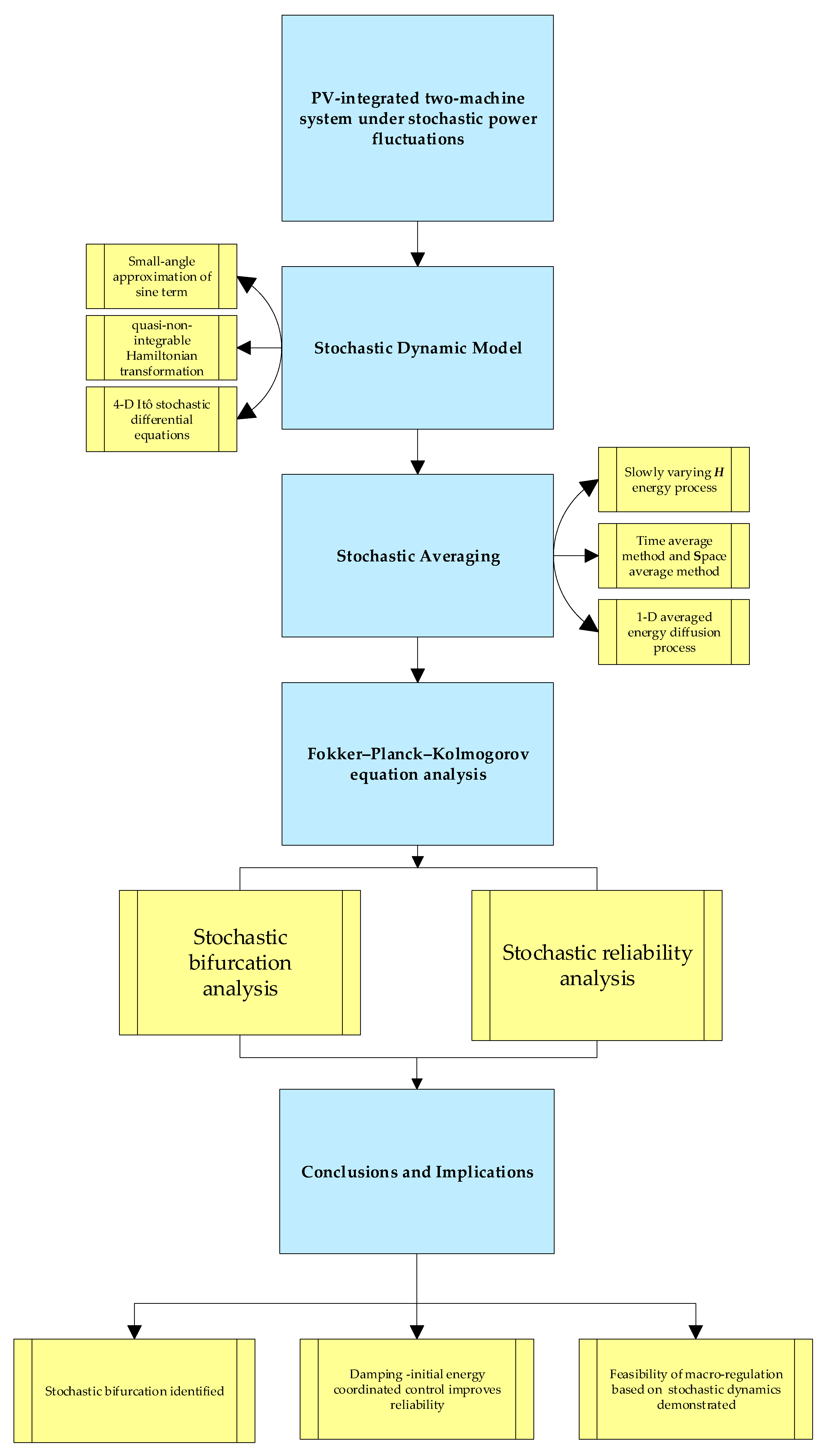Finally, Section 6 concludes the paper and outlines future research directions. The research flowchart is shown in Figure 1.

2. Stochastic Dynamic Model of the Four-Dimensional Motor System

Consider the following two-degree-of-freedom four-dimensional nonlinear motor system excited by stochastic noise:

$$\left\{\begin{array}{l}{\dot{\delta }}_1={\omega }_1\\ M_1{\dot{\omega }}_1=P_{m1}-D_1{\omega }_1-E_1{E}_2{Y}_{12}\sin ({\delta }_1-{\delta }_2)-k_1{\delta }_1-k_2{{\delta }_1}^3-{\xi }_{11}(t)-{\delta }_1{\xi }_{12}(t)\\ {\dot{\delta }}_2={\omega }_2\\ M_2{\dot{\omega }}_2=P_{m2}-D_2{\omega }_2-E_2{E}_1{Y}_{21}\sin ({\delta }_2-{\delta }_1)-{\delta }_2{\xi }_{22}(t)\end{array}\right.$$

(1)

where $\delta$ is the motor power angle, $\omega$ is the motor angular velocity, all in per-unit values. $M$ and $D$ are the inertia time constant and damping coefficient, respectively. $f({\delta }_1)=k_1{\delta }_1+k_2{{\delta }_1}^3$ is the nonlinear power angle control function. $P_{mi}$ is the mechanical power. ${\xi }_{ij}(t)$ is a Gaussian white noise stochastic process with zero mean and autocorrelation coefficient $R(\tau )=2{\sigma }_{ij}\delta (\tau )$, ${\sigma }_{ij}$ is the noise intensity, and the noises are independent of each other. Here, ${\xi }_{11}(t)$ represents the stochastic power fluctuation caused by external excitation, and ${\xi }_{12}(t)$ and ${\xi }_{22}(t)$ represent the stochastic disturbances accompanying the motor itself as the power angle changes.

The steady-state power angle difference in the two-machine system depends on the proportion of load shared by each, typically not too large. This is because a steadily operating motor system with a large power angle difference has a fragile static stability limit, such that sufficiently small disturbances can cause the rotor to accelerate, further widening the power angle difference, potentially leading to loss of synchronism and out-of-step incidents. Therefore, performing a series expansion on the electromagnetic power sine term in system (1):

$$\sin \left|{\delta }_1-{\delta }_2\right|=\left|{\delta }_1-{\delta }_2\right|-{\displaystyle \frac{{\left|{\delta }_1-{\delta }_2\right|}^3}{3!}}+{\displaystyle \sum _{n=2}^{\infty }\frac{{\left|{\delta }_1-{\delta }_2\right|}^{2n+1}}{(2n+1)!}}$$

(2)

The terms ${\displaystyle \sum _{n=2}^{\infty }\frac{{\left|{\delta }_1-{\delta }_2\right|}^{2n+1}}{(2n+1)!}}$ can be omitted as higher-order terms. When the power angle difference is small, the third-order term can be considered the main source of relative error $\epsilon$, retaining only the first-order term $\left|{\delta }_1-{\delta }_2\right|$. Here $\epsilon$ is defined as:

$$\epsilon ={\displaystyle \frac{\left|\sin \left|{\delta }_1-{\delta }_2\right|-\left|{\delta }_1-{\delta }_2\right|\right|}{\sin \left|{\delta }_1-{\delta }_2\right|}}={\displaystyle \frac{{\left|{\delta }_1-{\delta }_2\right|}^3}{6\sin \left|{\delta }_1-{\delta }_2\right|}}$$

(3)

Simultaneously, the system Equation (1) is finally approximated as:

$$\left\{\begin{array}{l}{\dot{\delta }}_1={\omega }_1\\ M_1{\dot{\omega }}_1=P_{m1}-D_1{\omega }_1-E_1{E}_2{Y}_{12}({\delta }_1-{\delta }_2)-k_1{\delta }_1-k_2{{\delta }_1}^3-{\xi }_{11}(t)-{\delta }_1{\xi }_{12}(t)\\ {\dot{\delta }}_2={\omega }_2\\ M_2{\dot{\omega }}_2=P_{m2}-D_2{\omega }_2-E_2{E}_1{Y}_{21}({\delta }_2-{\delta }_1)-{\delta }_2{\xi }_{22}(t)\end{array}\right.$$

(4)

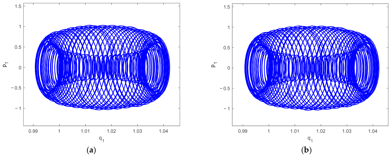
The smaller the relative error $\epsilon$, the more accurate the approximation. Figure 2 shows the comparison of two-dimensional phase trajectories between the original system (1) and the approximate system (4).

Figure 2 is essential for validating the small-angle engineering approximation employed in this study. The original system (1) contains a sinusoidal nonlinearity in the electromagnetic power term, which hinders direct Hamiltonian modeling and stochastic averaging. By assuming a small power-angle difference, the sine function is expanded and only the linear term is retained, producing the approximate system (4).

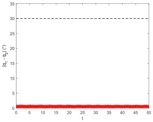
The significance of Figure 2 is twofold. First, the phase trajectories of the original and approximate systems in the $q_1$-$p_1$ plane nearly coincide, indicating that the approximation does not alter the qualitative dynamical structure of the system. Second, Figure 3 demonstrates that the power-angle difference $\epsilon$ stays below 0.3 rad throughout the simulation, which corresponds to a relative error as defined in Equation (3) of less than 5%, confirming that the quantitative error remains within an acceptable range. These results verify that the small-angle linearization does not distort the fundamental phase-space geometry of the system, thus supplying a reliable premise for the subsequent quasi-non-integrable-Hamiltonian transformation, stochastic averaging, and analytical solutions.

Let ${\delta }_1=q_1$, ${\delta }_2=q_2$, $M_1{\omega }_1=p_1$, $M_2{\omega }_2=p_2$. System (4) is transformed into the following Hamiltonian form:

$$\left\{\begin{array}{l}{\dot{q}}_1={\displaystyle \frac{1}{M_1}}{p}_1\\ {\dot{p}}_1=P_{m1}-{\displaystyle \frac{D_1}{M_1}}{p}_1-\left(k_e+k_1\right)q_1+k_e{q}_2-k_2{q_1}^3-{\xi }_{11}(t)-q_1{\xi }_{12}(t)\\ {\dot{q}}_2={\displaystyle \frac{1}{M_2}}{p}_2\\ {\dot{p}}_2=P_{m2}-{\displaystyle \frac{D_2}{M_2}}{p}_2+k_e{q}_1-k_e{q}_2-q_2{\xi }_{22}(t)\end{array}\right.$$

(5)

where $k_e=E_1{E}_2{Y}_{12}$, and the circuit mutual admittance $Y_{12}=Y_{21}$. Due to the presence of damping and excitation, system (5) is non-conservative. When the difference between the total dissipated damping energy and the input external excitation energy is much smaller than the system’s conservative energy, the system can be regarded as a quasi-Hamiltonian system [27]. The total system energy, i.e., the Hamiltonian H, can be calculated as:

$$H={\displaystyle \frac{1}{2}}{\displaystyle \frac{{p_1}^2}{M_1}}+{\displaystyle \frac{1}{2}}{\displaystyle \frac{{p_2}^2}{M_2}}+U(q_1,q_2)$$

(6)

where the potential energy term is

$$U(q_1,q_2)=-P_{m1}{q}_1-P_{m2}{q}_2+{\displaystyle \frac{E_1{E}_2{Y}_{12}}{2}}{q_1}^2+{\displaystyle \frac{E_1{E}_2{Y}_{12}}{2}}{q_2}^2-E_1{E}_2{Y}_{12}{q}_1{q}_2+{\displaystyle \frac{k_1}{2}}{q_1}^2+{\displaystyle \frac{k_2}{4}}{q_1}^4$$

(7)

The quasi-non-integrable Hamiltonian system constructed by Equations (6) and (7) can be transformed into a set of Itô-type stochastic differential equations:

$$\left\{\begin{array}{l}d{q}_1={\displaystyle \frac{\partial H}{\partial p_1}}dt\\ d{p}_1=-({\displaystyle \frac{\partial H}{\partial q_1}}+D_1{\displaystyle \frac{\partial H}{\partial p_1}})dt-d{B}_{11}(t)-q_{1}d{B}_{12}(t)\\ d{q}_2={\displaystyle \frac{\partial H}{\partial p_2}}dt\\ d{p}_2=-({\displaystyle \frac{\partial H}{\partial q_2}}+D_2{\displaystyle \frac{\partial H}{\partial p_2}})dt-q_{2}d{B}_{22}(t)\end{array}\right.$$

(8)

$B_{ij}(t)$ is a Wiener process satisfying $d{B}_{ij}(t)={\xi }_{ij}(t)dt$. The Wong–Zakai correction terms for system (8) can be described as [28]:

$$f_{wzij}={\displaystyle \frac{1}{2}}·{\sigma }_{ij}(q_i,p_i)·{\displaystyle \frac{\partial {\sigma }_{ij}(q_i,p_i)}{\partial p_i}}$$

For example, for the diffusion term $q_1$ of $B_{12}(t)$, its Wong–Zakai correction term satisfies:

$$\begin{array}{ll}{f}_{wz12}& ={\displaystyle \frac{1}{2}}·q_1·{\displaystyle \frac{\partial q_1}{\partial p_1}}\\ & =0\end{array}$$

(9)

It is easy to see that this holds for every Wiener process in system (8).

3. Stochastic Averaging Method

According to Itô’s lemma [29], the system energy can be expressed as the following Itô stochastic differential equation:

$$\begin{array}{c}dH=\left[-{\displaystyle \frac{D_1}{{M_1}^2}}{p_1}^2-{\displaystyle \frac{D_2}{{M_2}^2}}{p_2}^2+{\displaystyle \frac{{\sigma }_{12}}{M_1}}{q_1}^2+{\displaystyle \frac{{\sigma }_{22}}{M_2}}{q_2}^2+{\displaystyle \frac{{\sigma }_{11}}{M_1}}\right]dt\\ -{\displaystyle \frac{1}{M_1}}{p}_{1}d{B}_{11}(t)-{\displaystyle \frac{1}{M_1}}{q}_1{p}_{1}d{B}_{12}(t)-{\displaystyle \frac{1}{M_2}}{q}_2{p}_{2}d{B}_{22}(t)\end{array}$$

(10)

The detailed derivation of Equation (10) is in Appendix A.

Based on previous assumptions, the damping dissipation, stochastic disturbances, and stochastic PV excitation on the system are small, with noise intensity ${\sigma }_{ij}$ and damping coefficient D being of small order. Therefore, $H=H(q_i,p_i)$ can be regarded as a slowly varying process. Khasminskii’s theorem [30] indicates that under these conditions, the system energy H weakly converges to a one-dimensional Markov diffusion process. Through stochastic averaging, we obtain:

$$dH=\overline{m}(H)dt+\overline{\sigma }(H)dB(t)$$

(11)

where $\overline{m}(H)$ is the drift coefficient, $\overline{\sigma }(H)$ is the diffusion coefficient, and B(t) is a standard Wiener process. They share the forms in Appendix B, according to which these two terms can be fully calculated.

4. Stochastic Bifurcation and Stochastic Reliability Analysis

The probability density distribution of the one-dimensional diffusion process obeys an analytical form given by the FPK equation. Therefore, both stochastic bifurcation and stochastic reliability analysis are based on the analytical solution of the FPK equation [31,32,33]. This section will study the system’s stochastic bifurcation and reliability level based on the forward and backward forms of the FPK equation.

The FPK equation corresponding to the one-dimensional diffusion process is:

$${\displaystyle \frac{\partial p}{\partial t}}+{\displaystyle \frac{\partial }{\partial H}}\left[\overline{m}(H)p\right]-{\displaystyle \frac{1}{2}}{\displaystyle \frac{{\partial }^2}{\partial H^2}}\left[{\overline{\sigma }}^2(H)p\right]=0$$

(12)

Let ${\displaystyle \frac{\partial p}{\partial t}}=0$; i.e., the probability density function evolves to a steady state, yielding the stationary probability density function $p_s(H)$:

$$p_s(H)={\displaystyle \frac{C}{{\overline{\sigma }}^2(H)}}\exp \left[{\displaystyle \int \frac{2\overline{m}(H)}{{\overline{\sigma }}^2(H)}dH}\right]$$

(13)

C is the normalization constant. Meanwhile, the system response’s joint probability density function is:

$$p_s(q_1,q_2,p_1,p_2)={\displaystyle \frac{p_s(H)}{T(H)}}{|}_{H=H(q_1,q_2,p_1,p_2)}$$

(14)

Furthermore, the marginal probability density distributions can be obtained:

$$p_s(q_1,p_1)={\displaystyle {\int }_{-\infty }^{+\infty }{\displaystyle {\int }_{-\infty }^{+\infty }{p}_s(q_1,q_2,p_1,p_2)d{q}_{2}d{p}_2}}$$

(15)

$$p_s(q_1)={\displaystyle {\int }_{-\infty }^{+\infty }{p}_s(q_1,p_1)d{p}_1}$$

(16)

We mainly discuss the bifurcation change in the one-dimensional diffusion process (11) near the left boundary [28]. When it is a static excitation, ${\sigma }_{11}=0$. After simplification and calculation [27], the one-dimensional diffusion process can be written as:

$$dH=\left[\left({\displaystyle \frac{7}{9}}{b}_1-{\displaystyle \frac{11}{3}}{D}_e\right)H-{\displaystyle \frac{5}{6}}{D}_e{b}_2{H}^2\right]dt+\sqrt{({\displaystyle \frac{13}{18}}{b}_3-{\displaystyle \frac{5}{3}}{b}_2)}HdB(t)$$

(17)

According to Equation (14), the corresponding $p_s(H)$ is:

$$p_s(H)={\displaystyle \frac{C}{K}}{H}^{{\displaystyle \frac{2A}{K}}-2}\exp \left(-{\displaystyle \frac{2B}{K}}H\right)$$

(18)

where

$$\begin{array}{l}A={\displaystyle \frac{7}{9}}{b}_1-{\displaystyle \frac{11}{3}}{D}_e,B={\displaystyle \frac{5}{6}}{D}_e{b}_2,\\ K={\displaystyle \frac{13}{18}}{b}_3-{\displaystyle \frac{5}{3}}{b}_2\end{array}$$

(19)

$$\begin{array}{l}{b}_1={\displaystyle \frac{\frac{{\sigma }_{12}}{M_1}{P_{m2}}^2+\frac{{\sigma }_{22}}{M_2}{P_{m1}}^2}{k_e{(P_{m1}+P_{m2})}^2+k_1{P_{m2}}^2}}, \\ b_2={\displaystyle \frac{k_2{P_{m2}}^4}{{\left[k_e{\left(P_{m1}+P_{m2}\right)}^2+k_1{P_{m2}}^2\right]}^2}},\\ b_3={\displaystyle \frac{{\sigma }_{12}{P_{m2}}^2+{\sigma }_{22}{P_{m1}}^2}{k_e{(P_{m1}+P_{m2})}^2+k_1{P_{m2}}^2}},\\ D_{\mathrm{e}}={\displaystyle \frac{D_1}{M_1}}+{\displaystyle \frac{D_2}{M_2}}.\end{array}$$

(20)

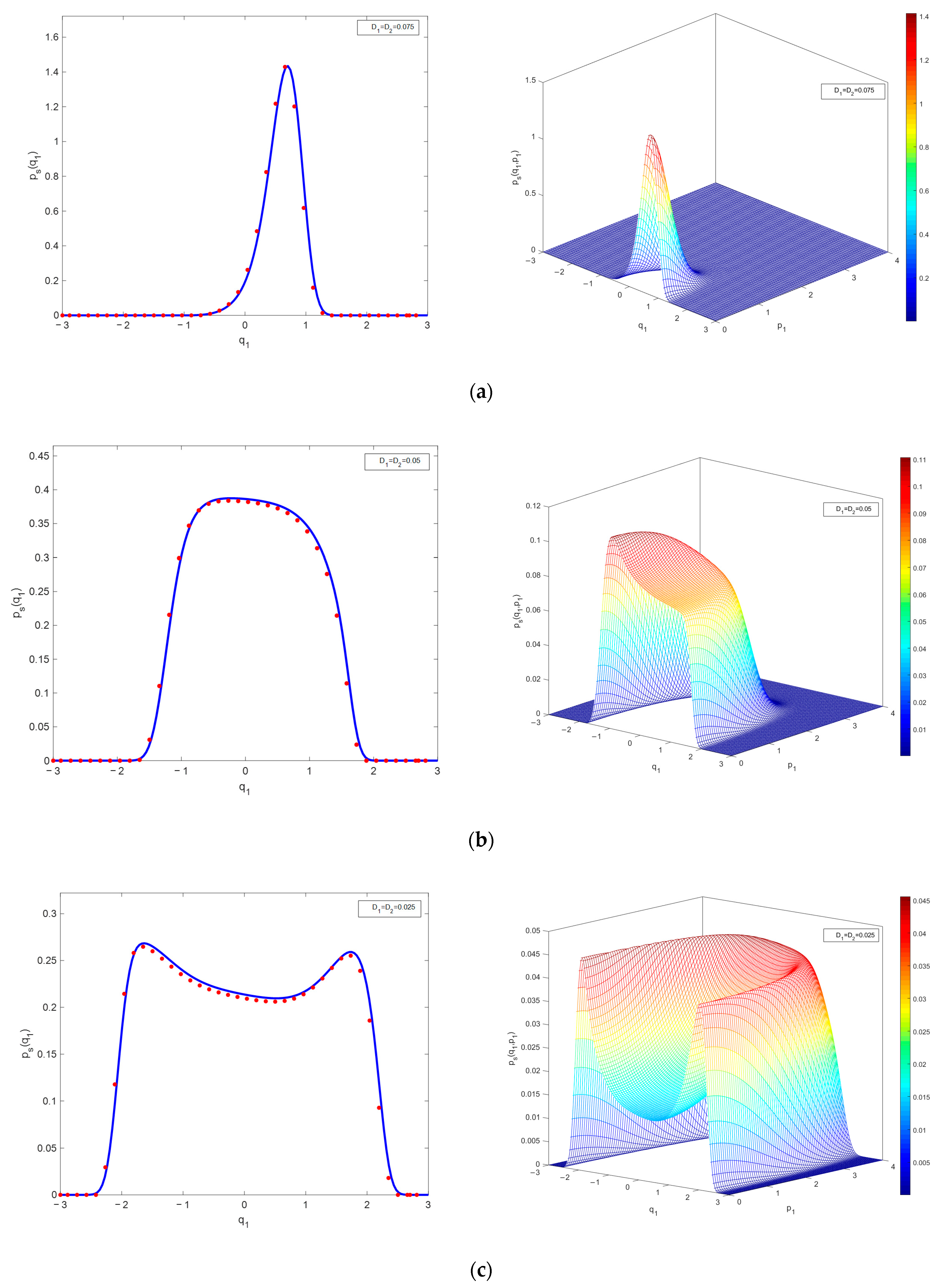
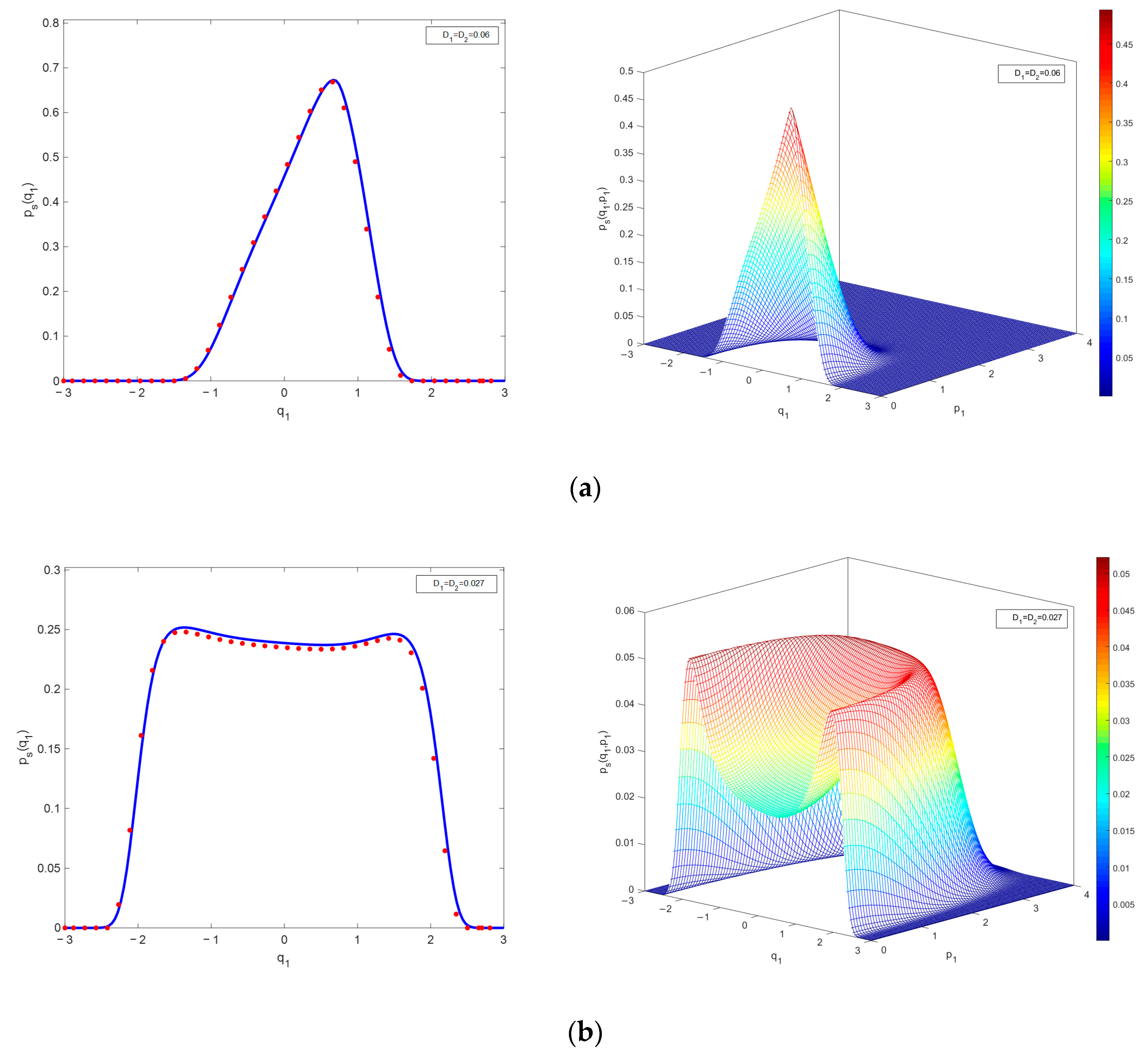
Substituting Equation (18) into Equation (14) yields the joint PDF $p_s(q_1,q_2,p_1,p_2)$, and one can obtain $p_s(q_1,p_1)$ and $p_s(q_1)$ according to Equations (16) and (17). Fix the parameters $M_1=M_2=0.23$, $P_{m1}=P_{m2}=1.5$, $E_1=E_2=1$, $Y_{12}=Y_{21}=1$, $k_1=1.2$, $k_2=6$, ${\sigma }_{12}={\sigma }_{22}=2$. Figure 4 shows the variation in the marginal probability density distribution with the damping coefficient. When $D_1=D_2=0.075$, the PDF is unimodal; decreasing the damping to $D_1=D_2=0.05$, and further to 0.025, the marginal PDF becomes bimodal, and the joint PDF becomes crater-shaped, indicating the occurrence of a P-bifurcation.

When it is a dynamic excitation, ${\sigma }_{11}\ne 0$. The one-dimensional diffusion process can be written as:

$$\begin{array}{c}dH=\left[\left({\displaystyle \frac{7}{9}}{b}_1-{\displaystyle \frac{11}{3}}{D}_{\mathrm{e}}\right)H-{\displaystyle \frac{5}{6}}{D}_e{b}_2{H}^2+{\displaystyle \frac{{\sigma }_{11}}{M_1}}\right]dt\\ +\sqrt{{\displaystyle \frac{22}{3}}{\sigma }_{11}H+({\displaystyle \frac{13}{18}}{b}_3-{\displaystyle \frac{5}{3}}{b}_2)H^2}dB(t)\end{array}$$

(21)

According to Equation (13), the corresponding $p_s(H)$ is:

$$p_s(H)=C{H}^{\left({\displaystyle \frac{3}{11M_1}}-1\right)}{\left({\displaystyle \frac{22}{3}}{\sigma }_{11}+KH\right)}^{\lambda }\exp \left(-{\displaystyle \frac{2B}{K}}H\right)$$

(22)

where

$$\lambda ={\displaystyle \frac{2A}{K}}-{\displaystyle \frac{3}{11M_1}}{\displaystyle \frac{B}{K}}+{\displaystyle \frac{22{\sigma }_{11}}{3}}{\displaystyle \frac{B}{K^2}}-1$$

(23)

The parameters A, B, K are given by (19), and their original specific forms are given by (20). Applying the steps from Equation (15) to (16) yields $p_s(q_1,p_1)$ and $p_s(q_1)$. Fix the parameters $M_1=0.13$,$M_2=0.23$, $P_{m1}=P_{m2}=1.5$, $E_1=E_2=1$, $Y_{12}=Y_{21}=1$, $k_1=1.2$, $k_2=6$, ${\sigma }_{12}={\sigma }_{22}=2$, ${\sigma }_{11}=1$. Figure 5 shows the variation in its marginal probability density distribution with the damping coefficient. When $D_1=D_2=0.06$, the damping is at a relatively strong level, $p_s(q_1)$ and $p_s(q_1,p_1)$ exhibit unimodal distributions; Decreasing the damping to $D_1=D_2=0.027$, a clear bimodal structure appears in $p_s(q_1)$, and $p_s(q_1,p_1)$ becomes crater-shaped. This indicates that under the combined action of dynamic photovoltaic excitation and stochastic power angle disturbance, damping changes can still cause the system to exhibit stochastic bifurcation behavior.

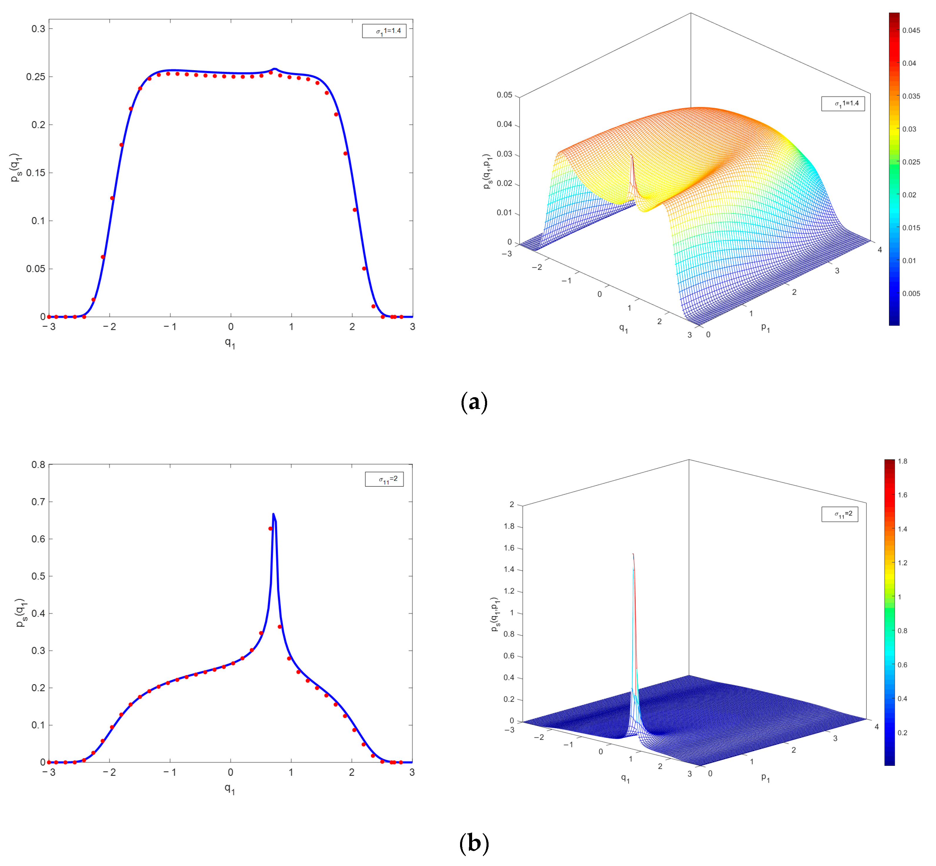
Figure 6 shows the effect of external excitation intensity ${\sigma }_{11}$ on the PDF. Here $D_1$ and $D_2$ are fixed at 0.027, $M_1$ is increased to 0.23, and other parameters remain unchanged. When ${\sigma }_{11}=1.4$, the originally bimodal structure of $p_s(q_1)$ changes, generating a new sharp peak. Further increasing ${\sigma }_{11}$ to 2 causes the small peaks on both sides of the sharp peak to degenerate, eventually evolving into a single unique sharp peak. Therefore, it can be said that as the external excitation intensity changes, the system’s motion behavior pattern transitions from a single limit cycle to one limit cycle and one attractor, and finally to the δ function. As can be seen from Figure 6, strong noise destroys the limit cycle structure of the system, which causes the “crater-shaped” potential well in Figure 4 to no longer exist. For general stochastic systems, the δ function implies a return to a deterministic state. However, at this point, the system’s damping dissipation can no longer compensate for the increase in random excitation. Therefore, in practical engineering, the influence of strong noise on power systems should be avoided.

In summary, for the system in this paper, whether under parameter excitation or combined external and parameter excitation, parameter changes can lead to stochastic bifurcation occurrence, and the bifurcation scenarios are more varied in the latter case. Additionally, due to the presence of the mechanical power term in the rotor motion equation, both excitation cases exhibit imperfect bifurcation characteristics, with the bimodal peaks showing height misalignment, which is particularly evident in Figure 4b.

5. Stochastic Reliability

Although stochastic stability analysis can describe the system’s motion behavior near the left boundary, it is still insufficient to fully explain the system’s reliability level under combined parameter and external excitation. Due to the influence of stochastic external excitation, the system’s Hamiltonian H still has the possibility of exceeding an engineering-acceptable reliability margin $H_{\mathrm{c}}$. Li and Ju [34] discussed this as the system’s “bounded fluctuation domain”. Therefore, “stochastic reliability” can be interpreted as: the probability that the system, under a certain initial condition $H_0$, remains within the “bounded fluctuation domain” ${\Omega }_H=\left(0,H_c\right]$ over time; i.e.,

$$R(t\left|H_0\right.)=P\left\{\left.H(s)\in {\Omega }_H,s\in \left(0,t\right]\right|\right.\left.H\left(0\right)=H_0\right\}$$

(24)

The backward form of the FPK equation:

$${\displaystyle \frac{\partial R}{\partial t}}=\overline{m}(H_0){\displaystyle \frac{\partial R}{\partial H_0}}+{\displaystyle \frac{1}{2}}{\overline{\sigma }}^2\left(H_0\right){\displaystyle \frac{{\partial }^{2}R}{\partial {H_0}^2}}$$

(25)

can be used to describe the reliability problem characterized by Equation (24). Since the actual system (5) involves both parameter and external excitation, the boundary conditions for Equation (25) should satisfy:

$$\left\{\begin{array}{l}R(0\left|H_0\right.)=1, H_0\in {\Omega }_H\\ R(t\left|H_c\right.)=0\\ {\displaystyle \frac{\partial R}{\partial t}}=\overline{m}\left(H_0\right){\displaystyle \frac{\partial R}{\partial H_0}}, H_0=0\end{array}\right.$$

(26)

This represents that the system is completely reliable at time zero. As time passes, the reliability function $R(t\left|H_0\right.)$ becomes 0 upon touching the boundary $H=H_{\mathrm{c}}$. Furthermore, the reliability decay rate, i.e., the conditional probability density $p\left(t\left|H_0\right.\right)$, is:

$$p\left(t\left|H_0\right.\right)=-{\displaystyle \frac{\partial R\left(t\left|H_0\right.\right)}{\partial t}}$$

(27)

We take $H_{\mathrm{c}}=0.47$ as the failure boundary of the system’s “bounded fluctuation domain” to analyze the system’s stochastic reliability. Then the reliability index can be set as

$$R(t\left|H_0\right.)=P\left\{\left.H(s)\in {\Omega }_H,s\in \left(0,t\right]\right|\right.\left.H\left(0\right)=H_0\right\}$$

Fixing $D_{\mathrm{e}}=0.08$, the statistics of reliability can be seen in

Table 1. Statistics of reliability function R (%) with fixed damping coefficient D_e = 0.08.

	t(s)	0.5	1	1.5	2	5	10	20	30
H0
0.05		99.98	99.94	99.67	99.22	96.12	92.29	85.84	79.88
0.1		99.97	99.43	98.38	97.17	91.91	87.56	81.36	75.71
0.19		98.78	94.82	91.34	88.65	80.68	76.11	70.62	65.73
0.26		92.82	84.56	79.50	76.16	67.78	63.62	59.01	54.92
0.33		76.20	65.81	60.76	57.66	50.55	47.29	43.85	40.81

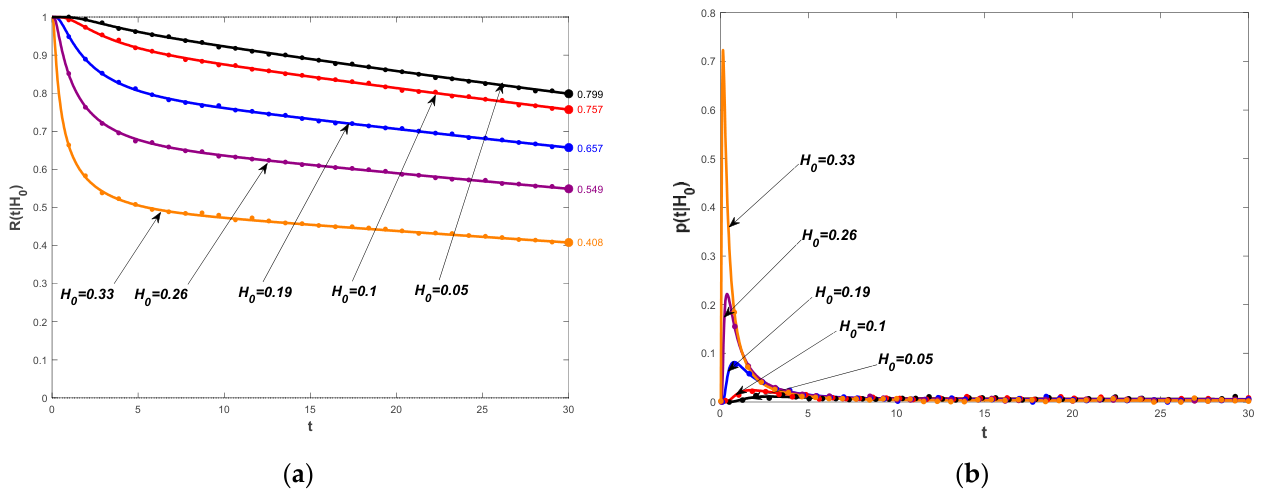
. The decreasing of reliability means the probability of the system staying in the “bounded fluctuation domain” is dropping as time moves on. We can see from Figure 7 and Table 1 that the function R decreases very rapidly at the beginning and then slows down as time progresses. From Table 1 we also know that for a certain initial energy level, e.g., $H_0$ = 0.33, it only takes 5 s for R to decrease to 50%. Figure 7 shows the decay of reliability over time under different initial energies $H_0$. Higher initial energy necessarily leads to a rapid decay in reliability. However, we find that compared to higher initial energy levels, when the initial energy is 0.05 or 0.1, the reliability hardly decreases over time, as shown in Figure 6a; when the initial energy reaches 0.19 or higher, the reliability drops quickly without much time, a phenomenon more clearly observed in Figure 6b, in which the peak of the probability density function arrives faster and is steeper as initial energy increases. Therefore, controlling the initial energy within a certain interval is necessary, as the system’s reliability decline is more gradual, allowing more time margin for fault detection.

Additionally, the damping coefficient also significantly affects stochastic reliability. Fixing $H_0=0.05$, then the reliability index can be set as

$$R(t\left|H_0\right.)=P\left\{\left.H(s)\in {\Omega }_H,s\in \left(0,t\right]\right|\right.\left.H\left(0\right)=0.05\right\}$$

The decreasing of reliability with a fixed initial energy level can be seen in

Table 2. Statistics of reliability function R (%) with fixed initial energy H₀ = 0.05.

	t(s)	1	5	10	20	30
De
0.08		99.94	96.12	92.28	85.84	79.88
0.05		99.91	93.22	86.29	75.16	65.53
0.02		99.83	88.86	77.68	60.89	47.86

. Comparing Table 1 and Table 2, we can see that variations in the damping coefficient $D_{\mathrm{e}}$ have a milder effect on R. In contrast, variations in the initial energy level $H_0$ have a more significant impact on R. Nevertheless, this difference is significant only at the early stage of the process (t < 10 s). For instance, during the same transient period from 0 to 10 s, R drops by 53% for $H_0$ = 0.33 in Table 1, whereas it drops by 23% for $D_{\mathrm{e}}$ = 0.02 in Table 2. Beyond 10 s, the effects of both $D_{\mathrm{e}}$ and $H_0$ on R become approximately linear, meaning that R decreases at an almost uniform rate over time. This suggests that for the stochastic reliability function R, controlling $H_0$ should be given higher priority than controlling parameter $D_{\mathrm{e}}$.

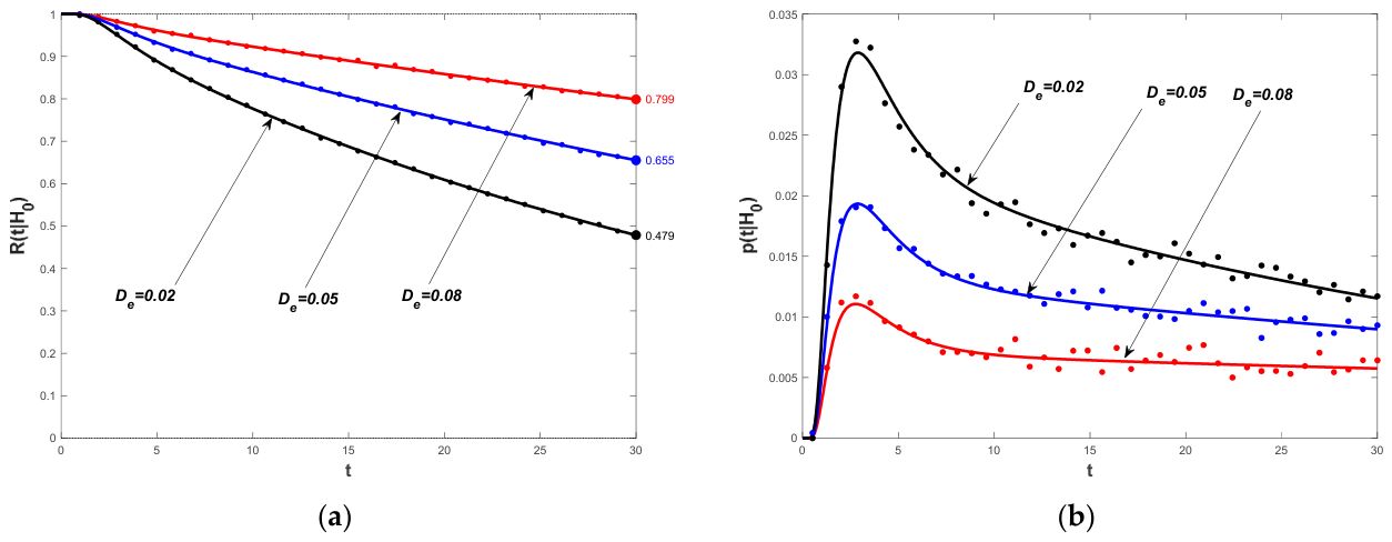
Figure 8 shows the system’s reliability under different damping coefficients $D_{\mathrm{e}}$. It can be seen that a higher damping coefficient helps improve the system’s stochastic reliability, making its decline over time slower; However, higher damping implies more energy loss. Therefore, comprehensive mixed regulation of $D_{\mathrm{e}}$ and $H_0$ can be performed. Comparing the blue curve $(H_0,D_{\mathrm{e}})=(0.05,0.05)$ in Figure 8a with the blue curve $(H_0,D_{\mathrm{e}})=(0.19,0.08)$ in Figure 7a, the final reliability decay degree of these two curves is almost equivalent at t = 30, because the larger damping compensates for the excessive decay trend caused by the larger initial energy. Similarly, to maintain stochastic reliability under smaller damping conditions, the magnitude of the initial energy $H_0$ should be reduced. Therefore, we can summarize that in the motor rotor motion system (8) under combined parameter and external excitation, stochastic reliability is influenced by parameters such as the damping coefficient and initial energy, which together organize the system’s motion behavior within the “bounded fluctuation domain”.

6. Conclusions

Based on the stochastic averaging principle, this paper has conducted several analyses on the stochastic bifurcation and reliability of a photovoltaic power system. Simulation results show that photovoltaic excitation and inherent power angle disturbances in the motor can lead to stochastic bifurcations in the power system. Particularly when both stochastic excitations act on the system simultaneously, the bifurcation behavior becomes more complex. Additionally, the study indicates that the system’s initial energy level and damping coefficient significantly impact its stochastic reliability, and controlling these two factors below certain thresholds can markedly enhance the system’s reliability level. All these phenomena demonstrate the feasibility of macro-regulation for power systems based on stochastic dynamics, and the effect of multi-parameter mixed regulation is superior to single-parameter regulation.

In recent years, some new stochastic averaging methods have been proposed. Studies on various types of random noise excitation [35] are also underway. The increasing penetration of renewable energy sources introduces more stochasticity into power grids [36]. Random fluctuations from renewable generation, load changes, and market behaviors are growing [37]. This trend calls for more analysis on stochastic behavior in dynamic systems. Traditional time averaging methods often require a clear separation of fast and slow time scales. However, in practice, this condition may not hold. To overcome this, we apply a stochastic averaging method to energy-space-based power systems. Unlike time averaging, we average over the system energy level. The system is first formulated as a Hamiltonian-like model. The total energy is treated as a slow variable. Fast oscillations are averaged out. This yields a reduced-order Itô stochastic differential equation for the energy dynamics. From this equation, we can obtain the probability density function of key system states. Our energy-space-based method can better capture the stochastic characteristics in nonlinear systems.

Our future research will focus on how to balance the fast and slow variations in different noises and how to introduce more refined noise models. More analysis can be conducted on completely integrable Hamiltonian systems and bifurcation behaviors in systems under various other types of noise excitation. Furthermore, the complete form of the FPK equation is a partial differential equation, and the bifurcation evolution behavior of the system governed by it can also be further discussed.