On the Joint Asymptotic Normality of the Method of Moments Estimators of the Two-Parameter Exponential Distribution

Abstract

Two-parameter exponential distribution has been widely used in research involving lifetime data, survival analysis, medical research, and reliability assessment. Since variables following this distribution are continuous, the population mean is often regarded as a key parameter of interest. In this paper, confidence intervals for the mean of a two-parameter exponential population are developed based on the joint asymptotic normality of the method of moments estimators, derived using the Delta method. The proposed asymptotic confidence intervals are compared with Wald-type confidence intervals in terms of coverage probability and average interval width. The performance of the proposed intervals is evaluated using Monte Carlo simulation, where particular attention is given to their coverage probability and mean interval width. The performance is further illustrated through a real-data application using daily PM2.5 concentration data from Bangkok, Thailand. Simulation, and the theoretical results indicate that the performance of estimators in the two-parameter exponential distribution improves as the sample size increases. Small samples lead to biased and unstable estimates, with wider confidence intervals and lower coverage probabilities, whereas moderate and large samples yield more accurate and stable results. For large samples, bias becomes negligible, variances approach the corresponding theoretical values, and coverage probabilities and interval widths approach the nominal level, confirming consistency and asymptotic efficiency.

1. Introduction

Statistical inference is widely used in applied research. Interval estimation is especially useful because it provides a range of possible values for the parameter of interest while considering sampling variability. Among the different parameters, the mean is often the main focus because it represents the expected value of the distribution and provides a simple summary of the population characteristics. Recent studies have further developed asymptotic inference for large-sample statistical analysis [1,2]. Nevertheless, the classical asymptotic framework under independent and identically distributed observations remains widely used in practical statistical inference.

Two-parameter exponential distribution has continuously developed and been widely applied across various fields, including reliability engineering [3], survival analysis [4], medicine [5], environmental research [6], economics, and actuarial science. For example, Barahona et al. apply a scale-mixture extension of the exponential distribution to repair-time data of airborne communications receivers [7]. Liyuan Pang et al. applied the logistic Truncated exponential skew logistic (LTESL) to three engineering datasets, including perforation measurements, component failure times, and aircraft air-conditioning system failures [8]. Reyes et al. applied the bimodal exponential distribution of vanadium concentration and flood peak exceedance data sets [9]. Collectively, these studies demonstrate the broad applicability of the distribution across diverse domains. More recently, interval estimation and parameter estimation methods for the two-parameter exponential distribution have continued to attract attention, reflecting the ongoing development of statistical inference for this distribution [10,11].

The wide range of applications of the two-parameter exponential distribution makes accurate parameter estimation particularly important. In this situation, interval estimation is important because it provides more information than a point estimate. Extensive research has investigated confidence interval estimation for the parameters of the two-parameter exponential distribution. For example, Roy and Mathew proposed an exact lower confidence limit for the reliability function of the two-parameter exponential distribution based on Type II censored data, using the generalized confidence interval approach. The study demonstrates that the proposed interval achieves the nominal coverage probability and provides a numerical procedure for its computation [12]. Subsequently, Fernández examined the generalized confidence limits for the reliability function of the two-parameter exponential distribution under failure censoring and addresses the issue that previously proposed limits may exceed unity [13]. Jiang and Wong developed exact and approximate significance functions for the scale and threshold parameters of the two-parameter exponential distribution via a renormalized $p^{*}$-formula and derived a predictive density function  [14]. Shi and Lin proposed generalized variable procedures for confidence intervals and hypothesis testing on the ratio and difference of mean lifetimes from two independent two-parameter exponential distributions [15]. Li et al. proposed a parametric bootstrap procedure to construct simultaneous confidence intervals for pairwise mean differences among multiple two-parameter exponential distributions [16]. More recently, Abdullahi and Phaphan introduced the Nakagami-Exponential distribution, a new extension of the exponential family with improved flexibility for modeling lifetime data. They investigated several theoretical and statistical properties of the proposed distribution, including parameter estimation and applications to real datasets [17].

In addition, a key issue lies in the selection of an efficient estimator, as the properties of an estimator directly affect the accuracy and reliability of the resulting confidence intervals. Various approaches have been proposed in the literature. In particular, Cohen and Helm derived a best linear unbiased estimator via an improved method of moments and evaluated its performance relative to maximum likelihood and other moment-based estimators [18]. Rahman and Pearson compared maximum likelihood estimator, unbiased linear estimators, product spacings, and quantile-based methods for parameter estimation in the two-parameter exponential distribution [19]. Rashid and Akhter investigated parameter estimation for the two-parameter exponential distribution in reliability analysis. Several estimation methods are compared, including least squares, relative least squares, ridge regression, moment-based estimators, and maximum likelihood variants [20]. Although previous studies have demonstrated substantial progress in estimation methods from multiple perspectives, the construction of confidence intervals for the population mean based directly on unbiased estimators has not been clearly addressed, particularly in the context of the two-parameter exponential distribution. Therefore, this study aims to develop confidence intervals derived from unbiased estimators of the scale and location parameters in order to fill the existing methodological gap.

The remainder of this paper is organized as follows. Section 2 presents the two-parameter exponential distribution, including its probability density function and moments. Section 3 describes the method of moments estimators for the scale and location parameters. Section 4 establishes the joint asymptotic normality of the Method of Moments (MoM) estimators via the Delta method. Section 5 derives the asymptotic properties of the population mean estimator. Section 6 describes the simulation study. Section 7 presents the simulation results and their comparison with the theoretical findings. Section 8 evaluates the accuracy of the asymptotic approximation. Section 9 illustrates the proposed method through a real-data application using PM2.5 data from Bangkok, Thailand. Finally, Section 10 concludes the paper.

2. Two-Parameter Exponential Distribution

2.1. Probability Density Function

Let $\mathrm{Expo}(\lambda ,\theta )$ denote the two-parameter exponential distribution. The probability density function of the two-parameter exponential distribution is given by

$$f(x;\lambda ,\theta )=\left\{\begin{array}{cc}{\displaystyle \frac{1}{\lambda }}exp\left\{-{\displaystyle \frac{x-\theta }{\lambda }}\right\},\hfill & \mathrm{if}x>\theta ,\hfill \\ 0,\hfill & \mathrm{otherwise},\hfill \end{array}\right.$$

(1)

where $\lambda >0$ and $\theta \in \mathbb{R}$ denote a scale parameter and a location parameter, respectively.

2.2. Raw Moments

Let random variable $X\sim \mathrm{Expo}(\lambda ,\theta )$ and $n\in \mathbb{N}$. Straightforward application of the binomial formula and Gamma function gives the raw moments of the two-parameter exponential distribution as follows:

$$\begin{array}{c}\hfill \begin{array}{c}\hfill \mathbb{E}\left[X^n\right]={\displaystyle \sum _{j=0}^n}{\displaystyle \frac{n!}{(n-j)!}}{\lambda }^j{\theta }^{n-j},\end{array}\end{array}$$

(2)

where

$$\Gamma \left(\alpha \right)={\int }_0^{\infty }{u}^{\alpha -1}{e}^{-u}du,\alpha >0.$$

Therefore, the first four raw moments can be expressed as follows:

$$\begin{array}{cc}\hfill \mathrm{For} n=1:\mathbb{E}\left[X\right]& =\lambda +\theta .\hfill \\ \hfill \mathrm{For} n=2:\mathbb{E}\left[X^2\right]& ={\theta }^2+2\lambda \theta +2{\lambda }^2.\hfill \\ \hfill \mathrm{For} n=3:\mathbb{E}\left[X^3\right]& ={\theta }^3+3{\theta }^2\lambda +6\theta {\lambda }^2+6{\lambda }^3.\hfill \\ \hfill \mathrm{For} n=4:\mathbb{E}\left[X^4\right]& ={\theta }^4+4{\theta }^3\lambda +12{\theta }^2{\lambda }^2+24\theta {\lambda }^3+24{\lambda }^4.\hfill \end{array}$$

2.3. Central Moments

Let $\mu =\mathbb{E}\left[X\right]=\lambda +\theta$. Applying the binomial formula, the central moments of the two-parameter exponential distribution can be calculated as follows:   

$$\begin{array}{c}\hfill \mathbb{E}{(X-\mu )}^n={\displaystyle \sum _{k=0}^n}{(-1)}^{n-k}\left({\displaystyle \genfrac{}{}{0pt}{}{n}{k}}\right)\mathbb{E}\left[X^k\right]{\mu }^{n-k}.\end{array}$$

(3)

The first four central moments of the two-parameter exponential distribution are required to establish the asymptotic normality of the method-of-moments (MoM) estimators.

$$\begin{array}{c}\hfill {\mu }_2={\sigma }^2={\lambda }^2,{\mu }_3=\mathbb{E}{(X-\mu )}^3=2{\lambda }^3,{\mu }_4=\mathbb{E}{(X-\mu )}^4=9{\lambda }^4,\end{array}$$

where ${\mu }_2,{\mu }_3,$ and ${\mu }_4$ denote the central moments of the distribution, not cumulants.

2.4. Statistical Properties

Several useful statistical properties of the two-parameter exponential distribution are summarized below. The cumulative distribution function (CDF), moment generating function (MGF), survival function, hazard rate function, and quantile function are given by

$$\begin{array}{c}\hfill \begin{array}{cc}\hfill F\left(x\right)& =1-exp\left(-{\displaystyle \frac{x-\theta }{\lambda }}\right),x>\theta ,\hfill \\ \hfill M_X\left(t\right)& ={\displaystyle \frac{e^{\theta t}}{1-\lambda t}},t<{\displaystyle \frac{1}{\lambda }},\hfill \\ \hfill S\left(x\right)& =exp\left(-{\displaystyle \frac{x-\theta }{\lambda }}\right),x>\theta ,\hfill \\ \hfill h\left(x\right)& ={\displaystyle \frac{1}{\lambda }},x>\theta ,\hfill \\ \hfill Q\left(p\right)& =\theta -\lambda ln(1-p),0<p<1.\hfill \end{array}\end{array}$$

In addition, the median, mode, coefficient of variation (CV), skewness, and kurtosis are

$$\mathrm{Median}=\theta +\lambda ln2,\mathrm{Mode}=\theta ,\mathrm{CV}={\displaystyle \frac{\lambda }{\lambda +\theta }},\mathrm{Skewness}=2,\mathrm{Kurtosis}=9.$$

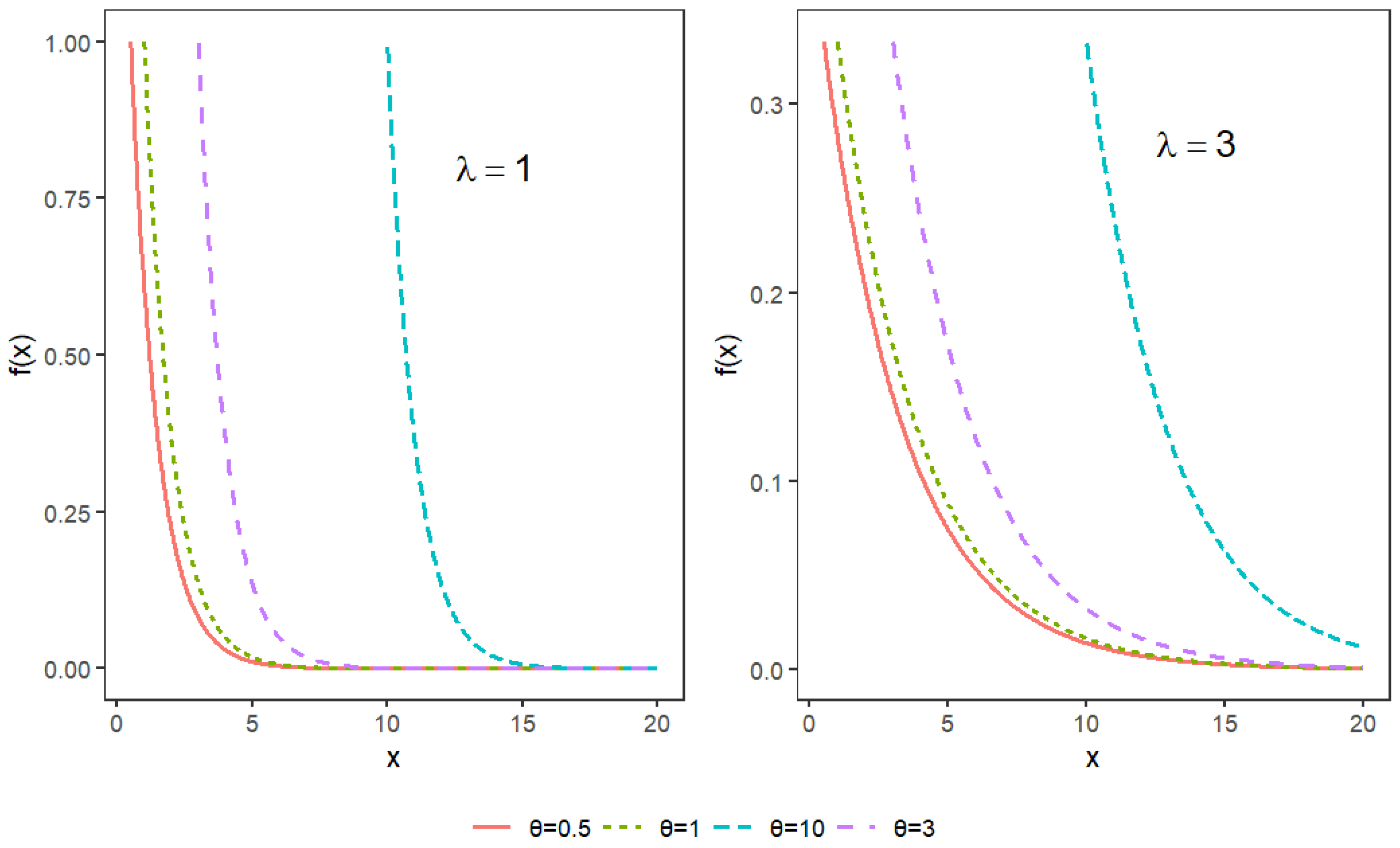
The shape of the distribution for various parameter values is illustrated in Figure 1.

3. Method of Moments Estimation

Although the maximum likelihood estimator (MLE) is generally asymptotically efficient; the MoM estimators for the two-parameter exponential distribution possess simple closed-form expressions that are directly related to the sample mean and sample variance. This simplicity facilitates the derivation of their joint asymptotic distribution through the Delta method. Moreover, the MoM estimators are asymptotically unbiased and consistent, providing a convenient basis for constructing asymptotic confidence intervals for the population mean. Let $X_1,X_2,\dots ,X_n$ be a sample from a population with the two-parameter exponential distribution. To estimate the parameters of this distribution using the MoM, the sample mean $\overline{X}$ and the sample variance $S^2$ are defined as follows:

$$\overline{X}={\displaystyle \frac{1}{n}}{\displaystyle \sum _{i=1}^n}{X}_i, \mathrm{and} S^2={\displaystyle \frac{1}{n-1}}{\displaystyle \sum _{i=1}^n}{(X_i-\overline{X})}^2.$$

The MoM involves equating the theoretical and sample moments. In this case, the MoM equations are expressed as

$$\begin{array}{cc}\hfill \mu =\lambda +\theta & =\overline{X},\hfill \\ \hfill {\sigma }^2={\lambda }^2& =S^2.\hfill \end{array}$$

Solving the system of equations for the unknown parameters $\lambda$ and $\theta$ yields the following MoM estimators, $\widehat{\lambda }$ and $\widehat{\theta }$:

$$\widehat{\lambda }=\sqrt{S^2},\widehat{\theta }=\overline{X}-\sqrt{S^2}.$$

(4)

4. Joint Asymptotic Normality of the MoM Estimators

According to the joint asymptotic normality [21,22], the random vector

$$\sqrt{n}\left(\begin{array}{c}\overline{X}-\mu \\ S^2-{\sigma }^2\end{array}\right)$$

converges in distribution as $n\to \infty$ to the bivariate normal distribution $N(\overrightarrow{0},\tilde{\Sigma })$, where $\overrightarrow{0}$ is the zero vector and $\tilde{\Sigma }$ is given by

$$\begin{array}{c}\hfill \tilde{\Sigma }=\left(\begin{array}{cc}{\sigma }^2& {\mu }_3\\ {\mu }_3& {\mu }_4-{\sigma }^4\end{array}\right)=\left(\begin{array}{cc}{\lambda }^2& 2{\lambda }^3\\ 2{\lambda }^3& 8{\lambda }^4\end{array}\right).\end{array}$$

(5)

Let $T_1=\overline{X}$ and $T_2=S^2$ be two basic statistics associated with the MoM estimators. The Delta method consists of expanding the functions $\widehat{\lambda }$ and $\widehat{\theta }$ of basic statistics into a two-dimensional Taylor series around the mathematical expectations $m_1$ and $m_2$ of $T_1$ and $T_2$ retaining only the linear terms, where

$$m_1=\mathbb{E}{T}_1=\mathbb{E}\overline{X}=\mu =\lambda +\theta , \mathrm{and} m_2=\mathbb{E}{T}_2=\mathbb{E}{S}^2={\sigma }^2={\lambda }^2.$$

(6)

From (4), the estimators $\widehat{\lambda }$ and $\widehat{\theta }$ can be expressed as functions of $\overline{X}$ and $S^2$ as follows:

$$\begin{array}{c}\hfill \widehat{\lambda }=g_1(\overline{X},S^2)=\sqrt{S^2},\widehat{\theta }=g_2(\overline{X},S^2)=\overline{X}-\sqrt{S^2},\end{array}$$

that is,

$$\begin{array}{c}\hfill g_1(t_1,t_2)=\sqrt{t_2} \mathrm{and} g_2(t_1,t_2)=t_1-\sqrt{t_2}\end{array}$$

Substituting $m_1$ and $m_2$ from (6), we obtain

$$g_1(m_1,m_2)=\sqrt{m_2}=\lambda \mathrm{and} g_2(m_1,m_2)=m_1-\sqrt{m_2}=(\lambda +\theta )-\sqrt{{\lambda }^2}=\theta .$$

Partial derivatives of $g_1(t_1,t_2)$ and $g_2(t_1,t_2)$ and there values evaluated at the mean points $m_1$ and $m_2$ are given as follows:

$$\begin{array}{c}\hfill \begin{array}{ccc}& {\displaystyle \frac{\partial g_1(t_1,t_2)}{\partial t_1}}=0,\hfill & \hfill {\displaystyle \frac{\partial g_1(m_1,m_2)}{\partial t_1}}=0,\\ & {\displaystyle \frac{\partial g_1(t_1,t_2)}{\partial t_2}}={\displaystyle \frac{1}{2\sqrt{t_2}}},\hfill & \hfill {\displaystyle \frac{\partial g_1(m_1,m_2)}{\partial t_2}}={\displaystyle \frac{1}{2\lambda }},\\ & {\displaystyle \frac{\partial g_2(t_1,t_2)}{\partial t_1}}=1,\hfill & \hfill {\displaystyle \frac{\partial g_2(m_1,m_2)}{\partial t_1}}=1,\\ & {\displaystyle \frac{\partial g_2(t_1,t_2)}{\partial t_2}}=-{\displaystyle \frac{1}{2\sqrt{t_2}}},\hfill & \hfill {\displaystyle \frac{\partial g_2(m_1,m_2)}{\partial t_2}}=-{\displaystyle \frac{1}{2\lambda }}.\end{array}\end{array}$$

Using the Delta method, the random vector ${\left(\widehat{\lambda },\widehat{\theta }\right)}^T$ is expanded into a two-dimensional Taylor series around $(m_1,m_2)$, retaining only the linear terms [22]. This yields

$$\begin{array}{c}\hfill \begin{array}{cc}\hfill \left(\begin{array}{c}\widehat{\lambda }\\ \widehat{\theta }\end{array}\right)& =\left(\begin{array}{c}{g}_1(T_1,T_2)\\ g_2(T_1,T_2)\end{array}\right)\hfill \\ & =\left(\begin{array}{c}{g}_1(m_1,m_2)\\ g_1(m_1,m_2)\end{array}\right)+\left(\begin{array}{cc}{\displaystyle \frac{\partial g_1(m_1,m_2)}{\partial t_1}}& {\displaystyle \frac{\partial g_1(m_1,m_2)}{\partial t_2}}\\ {\displaystyle \frac{\partial g_2(m_1,m_2)}{\partial t_1}}& {\displaystyle \frac{\partial g_2(m_1,m_2)}{\partial t_2}}\end{array}\right)\left(\begin{array}{c}{T}_1-m_1\\ T_2-m_2\end{array}\right)+\mathrm{Remainder}\hfill \\ & =\left(\begin{array}{c}\lambda \\ \theta \end{array}\right)+\left(\begin{array}{cc}0& {\displaystyle \frac{1}{2\lambda }}\\ 1& -{\displaystyle \frac{1}{2\lambda }}\end{array}\right)\left(\begin{array}{c}\overline{X}-(\lambda +\theta )\\ S^2-{\lambda }^2\end{array}\right)+\mathrm{Remainder}.\hfill \end{array}\end{array}$$

Moreover, $\sqrt{n}\mathrm{Remainder}\to \overrightarrow{0}$ in probability as the sample size $n\to \infty$. Therefore, the random vector $\sqrt{n}\left(\begin{array}{c}\widehat{\lambda }-\lambda \\ \widehat{\theta }-\theta \end{array}\right)$ converges to $N(\overrightarrow{0},\Sigma )$ as $n\to \infty$, where the covariance matrix is given by $\Sigma =B\tilde{\Sigma }{B}^{\prime }$, where the Jacobian matrix and the covariance matrix of the basic statistics $\overline{X}$ and $S^2$ are

$$\begin{array}{c}\hfill B=\left(\begin{array}{cc}0& {\displaystyle \frac{1}{2\lambda }}\\ 1& -{\displaystyle \frac{1}{2\lambda }}\end{array}\right).\end{array}$$

(7)

The simple multiplication of matrices in Equations (5) and (7) gives

$$\begin{array}{c}\hfill \Sigma =B\tilde{\Sigma }{B}^{\prime }=\left(\begin{array}{cc}0& {\displaystyle \frac{1}{2\lambda }}\\ 1& -{\displaystyle \frac{1}{2\lambda }}\end{array}\right)\left(\begin{array}{cc}{\lambda }^2& 2{\lambda }^3\\ 2{\lambda }^3& 8{\lambda }^4\end{array}\right)\left(\begin{array}{cc}0& 1\\ {\displaystyle \frac{1}{2\lambda }}& -{\displaystyle \frac{1}{2\lambda }}\end{array}\right)=\left(\begin{array}{cc}2{\lambda }^2& -{\lambda }^2\\ -{\lambda }^2& {\lambda }^2\end{array}\right).\end{array}$$

(8)

Therefore, the estimator $\widehat{\lambda }$ is asymptotically normal with

$$\mathrm{Asymptotic} \mathrm{mean}\left(\widehat{\lambda }\right)=\lambda ,\mathrm{Asymptotic} \mathrm{variance}\left(\widehat{\lambda }\right)=2{\lambda }^2.$$

Similarly, the estimator $\widehat{\theta }$ is asymptotically normal with

$$\mathrm{Asymptotic} \mathrm{mean}\left(\widehat{\theta }\right)=\theta ,\mathrm{Asymptotic} \mathrm{variance}\left(\widehat{\theta }\right)={\lambda }^2.$$

Moreover, the asymptotic covariance between $\widehat{\lambda }$ and $\widehat{\theta }$ is

$$\mathrm{Asymptotic} \mathrm{Cov}(\widehat{\lambda },\widehat{\theta })=-{\lambda }^2.$$

The mathematical rigorous statement is as follows:

Proposition 1. 

The method of moments estimators $\widehat{\lambda }=\sqrt{S^2}$ and $\widehat{\theta }=\overline{X}-\sqrt{S^2}$ of the parameters λ and θ of the two-parameter exponential distribution are jointly asymptotically normal with mean ${(\lambda ,\theta )}^T$ (asymptotically unbiased) and covariance matrix $\Sigma =\left(\begin{array}{cc}2{\lambda }^2& -{\lambda }^2\\ -{\lambda }^2& {\lambda }^2\end{array}\right)$. That is,

$$\sqrt{n}\left(\begin{array}{c}\widehat{\lambda }-\lambda \\ \widehat{\theta }-\theta \end{array}\right)\to N\left(\left(\begin{array}{c}0\\ 0\end{array}\right),\left(\begin{array}{cc}2{\lambda }^2& -{\lambda }^2\\ -{\lambda }^2& {\lambda }^2\end{array}\right)\right).$$

5. Asymptotic Properties of the Mean

As the mean of the two-parameter exponential distribution is $\mu =\lambda +\theta$, we suggest the following plug-in estimator of the mean, applying the MoM estimators:

$$\widehat{\mu }=\widehat{\lambda }+\widehat{\theta }.$$

Note that $\widehat{\mu }$ is asymptotically normal as a sum of two jointly asymptotically normal statistics. The following are the parameters of the asymptotic normality

$$\mathrm{Asymptotic} \mathrm{Mean}\left(\widehat{\mu }\right)=\mathrm{Asymptotic} \mathrm{Mean}\left(\widehat{\lambda }\right)+\mathrm{Asymptotic} \mathrm{Mean}\left(\widehat{\theta }\right)=\lambda +\theta =\mu ,$$

and

$$\begin{array}{c}\hfill \begin{array}{cc}\hfill \mathrm{Asymptotic} \mathrm{Variance}\left(\widehat{\mu }\right)& =\mathrm{Asymptotic} \mathrm{Variance}(\widehat{\lambda }+\widehat{\theta })\hfill \\ & =\mathrm{Asymptotic} \mathrm{Variance}\left(\widehat{\lambda }\right)+\mathrm{Asymptotic} \mathrm{Variance}\left(\widehat{\theta }\right)\hfill \\ & +2\mathrm{Asymptotic} \mathrm{Cov}(\widehat{\lambda },\widehat{\theta })\hfill \\ & ={\lambda }^2.\hfill \end{array}\end{array}$$

Therefore, $\widehat{\mu }$ is asymptotically normal $N(\mu ,{\lambda }^2)$. Mathematically rigorous statement is as follows

Proposition 2. 

The method of moments estimator of the $\widehat{\mu }=\widehat{\lambda }+\widehat{\theta }$ of the mean of the two-parameter exponential distribution is asymptotically normal with mean $\mu =\lambda +\theta$ (asymptotically unbiased) and variance ${\tau }^2={\lambda }^2$. That is,

$$\sqrt{n}(\widehat{\mu }-\mu )\to N(\mu ,{\lambda }^2).$$

Obviously, we do not know the true population parameters $\lambda$ and $\theta$. Because of that, we use their MoM estimators and obtain the following estimators for the asymptotic mean and variance:

$$\widehat{\mu }=\widehat{\lambda }+\widehat{\theta },\widehat{{\lambda }^2}={\widehat{\lambda }}^2.$$

If the sample size n tends to infinity, then for a significance level $\alpha$,

$$\mathbb{P}\left(\right|\mu -\widehat{\mu }|\le z_{\alpha /2}\lambda )\approx 1-\alpha ,$$

where $z_{\alpha /2}$ is $1-\alpha /2$-quantile of the standard normal distribution. Replacing $\lambda$ by its MoM estimator $\widehat{\lambda }$, we obtain the asymptotic equality

$$\mathbb{P}\left(\right|\mu -\widehat{\mu }|\le z_{\alpha /2}\widehat{\lambda })\approx 1-\alpha .$$

Therefore, if the sample size goes to infinity, then the interval with the endpoints

$$\begin{array}{c}\hfill \left(1\mp {\displaystyle \frac{z_{\alpha /2}}{\sqrt{n}}}\right)\widehat{\lambda }+\widehat{\theta }\end{array}$$

(9)

is the asymptotic $(1-\alpha )$-confidence interval for the mean value $\mu$.

6. Simulations Study

Let u be a random variate from the uniform distribution on (0, 1). To generate a random variate x from the two-parameter exponential distribution with parameters $\lambda$ and $\theta$, the inverse transform method is employed. The cumulative distribution function is

$$\begin{array}{c}\hfill u=F\left(x\right)=1-exp\left\{-{\displaystyle \frac{x-\theta }{\lambda }}\right\}.\end{array}$$

(10)

Solving for x, we obtain

$$\begin{array}{c}\hfill x=\theta -\lambda ln(1-u).\end{array}$$

(11)

Note that $1-u$ is also a random variate from the uniform distribution on (0, 1). Hence, a random variate from the two-parameter exponential distribution with parameters $\lambda$ and $\theta$ can be generated by transforming uniform random variables using the following Algorithm 1.

Algorithm 1: Generate two-parameter exponential random variate.

Step 1: Generate $u\sim U(0,1)$ Step 2: Set $X=\theta -\lambda lnu$.

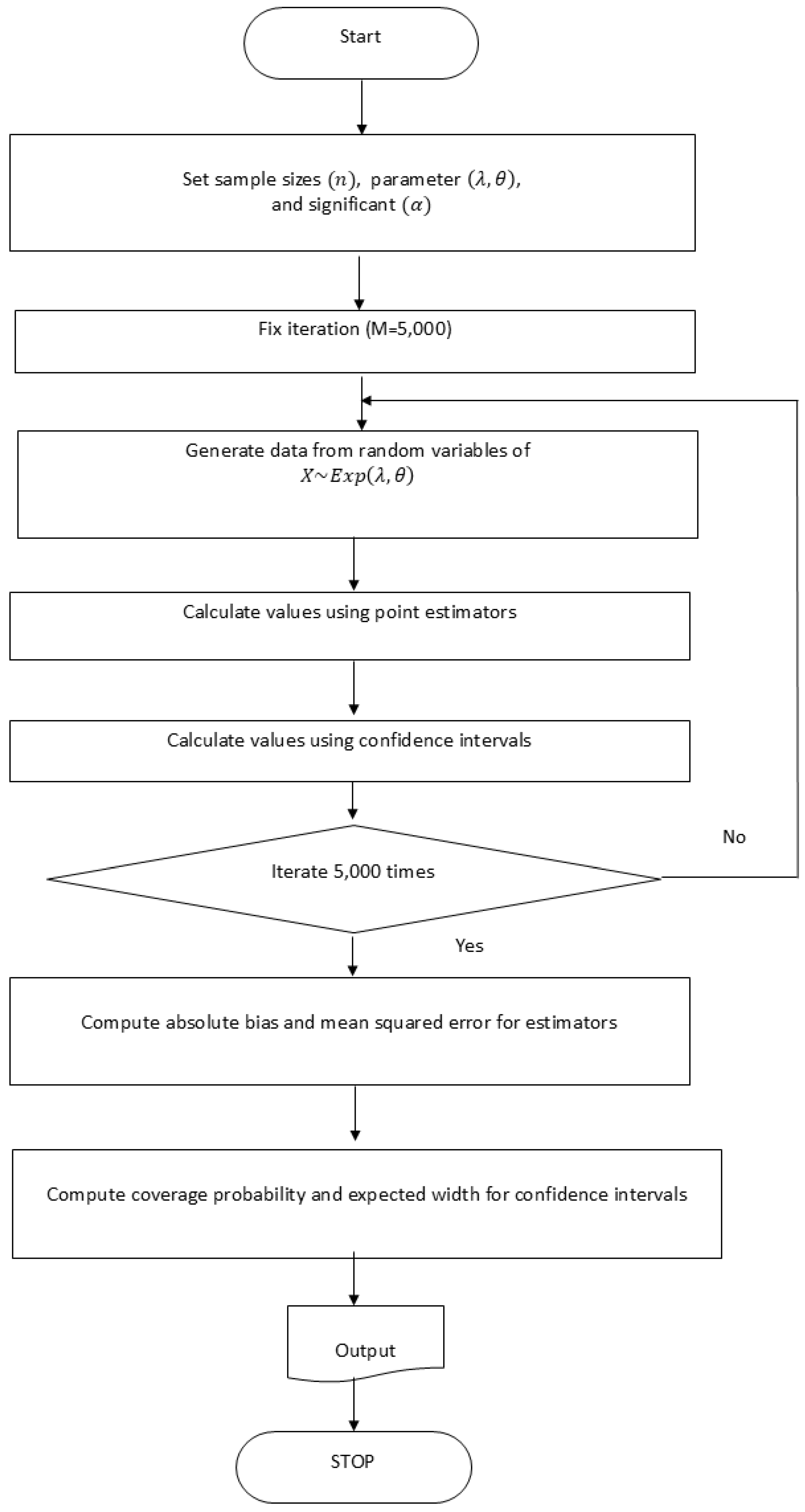
The simulation study compares the coverage probabilities and average lengths of confidence intervals for the population means of the two-parameter exponential distribution. Parameter values and sample sizes are specified, and the following steps are repeated a fixed number of times to obtain the desired results.

The parameter values were chosen to cover a range of distributional shapes and practical settings. The scale parameter $\lambda$ was set to 1 and 3 to represent low and moderate-to-high dispersion. The location parameter $\theta$ was computed as $\theta =\mu -\lambda$, where the population mean $\mu$ was fixed at 1.5, 2, 3.5, 4, 6, and 8, spanning small to large mean values commonly found in reliability, survival analysis, and environmental research. The resulting eight $(\lambda ,\theta )$ combinations provide a broad evaluation across realistic parameter settings. The population mean $\mu =\lambda +\theta$ is fixed at 1.5, 2, 3.5, 4, 6, and 8, reflecting small to large values and varying distributions. If $\lambda$ is fixed at 1 and 3, $\theta$ is computed by $\theta =\mu -\lambda$. Therefore, the values of $(\lambda ,\theta )$ are $(1,0.5)$, $(1,1)$, $(1,3)$, $(1,5)$, $(3,0.5)$, $(3,1)$, $(3,3)$, $(3,5)$. The sample size n is given as 10, 30, 50, 100, 200, and 500. The confidence level $(1-\alpha )$ is 0.95.

The simulation algorithm is as follows:

• Step 1: Fix parameters $\lambda$ and $\theta$, and sample size n.
• Step 2: Generate a sample of size n from the two-parameter exponential distribution.
• Step 3: Calculate the point estimator of parameters $\lambda$ and $\theta$ to obtain $\widehat{\lambda }$ and $\widehat{\theta }$ according to the formulae presented above. Obtain the mean estimator $\widehat{\mu }=\widehat{\lambda }+\widehat{\theta }$. Calculate the sample mean $\overline{x}$ and sample standard deviation s.
• Step 4: Compute $(1-\alpha )100\%$ asymptotic confidence intervals for mean $\mu$ according to the formulae above and denote lower and upper limits of the interval as $L^A$ and $U^A$, correspondingly.
• Step 5: Compute $(1-\alpha )100\%$ Wald confidence intervals for mean $\mu$ according to the formulae $\overline{x}\pm z_{\alpha /2}{\displaystyle \frac{s}{\sqrt{n}}}$, where $z_{\alpha /2}$ is the upper $\alpha /2$ quantile of the standard normal distribution, and denote lower and upper limits of the interval as $L^W$ and $U^W$, correspondingly.
• Step 6: Steps 1 to 6 are repeated for $M=5000$ times to obtain the 5000 estimators ${\widehat{\tau }}_i$ and confidence intervals limits $L_i^A$ and $U_i^A,i=1,2,\dots M$. This gives us M values of each characteristic ${\widehat{\mu }}_i,{\overline{x}}_i,s_i,L_i^A,U_i^A,L_i^W$, and $U_i^W,i=1,2,\dots ,M$.
• Step 7: The mean squared error (MSE) and absolute bias (ABS) for mean $\mu$ are computed by $MSE={\displaystyle \frac{1}{M}}{\sum }_{i=1}^M{({\widehat{\mu }}_i-\mu )}^2$ and $ABS={\displaystyle \frac{1}{M}}{\sum }_{i=1}^M|{\widehat{\mu }}_i-\mu |$.
• Step 8: For the asymptotic confidence interval, compute the average coverage probability (CP) and average interval width (AW) from $CP={\displaystyle \frac{\#(L_i^A\le \mu \le U_i^A)}{M}}$, and $AW={\displaystyle \frac{{\sum }_{i=1}^M(U_i^A-L_i^A)}{M}}$, where $\#(L_i^A\le \mu \le U_i^A)$ is the number of simulation runs for $\mu$ that lie within the confidence interval.

Similarly, for the Wald confidence interval, compute the average coverage probability and average interval width from $CP={\displaystyle \frac{\#(L_i^W\le \mu \le U_i^W)}{M}}$, and $AW={\displaystyle \frac{{\sum }_{i=1}^M(U_i^W-L_i^W)}{M}}$, where $\#(L_i^W\le \mu \le U_i^W)$ is the number of simulation runs for $\mu$ that lie within the Wald confidence interval.

Monte Carlo simulations are implemented in R to evaluate the coverage probabilities and expected lengths of the confidence intervals. The simulation framework is illustrated in Figure 2. In the final assessment, a method is considered preferable when its confidence interval attains a coverage probability close to the nominal level $(1-\alpha )$ while maintaining a relatively short interval length [21].

7. Comparing the Simulation and Asymptotic Results

The comparison between simulation and theoretical results indicates that for small sample sizes $n=10,30$ the estimators of $\lambda$ and $\theta$ are close to their true values but still exhibit slight biases, larger variances, and greater deviations in covariance, leading to less stable results, as shown in

Table 1. The simulation and results for small sample sizes.

			Simulation					Theory
$\mathit{n}$	$\widehat{\mathit{\lambda }}$	$\widehat{\mathit{\theta }}$	Mean ($\widehat{\mathit{\lambda }}$)	Mean ($\widehat{\mathit{\theta }}$)	Var ($\widehat{\mathit{\lambda }}$)	Var ($\widehat{\mathit{\theta }}$)	Covariance	Var ($\widehat{\mathit{\lambda }}$)	Var ($\widehat{\mathit{\theta }}$)	Covariance
10	1	0.5	0.9773	0.5236	0.1675	0.0689	−0.0679	0.2000	0.1000	−0.1000
10	1	1	0.9715	1.0273	0.1561	0.0657	−0.0630	0.2000	0.1000	−0.1000
10	1	3	0.9680	3.0315	0.1619	0.0694	−0.0656	0.2000	0.1000	−0.1000
10	1	10	0.9723	10.0281	0.1601	0.0688	−0.0641	0.2000	0.1000	−0.1000
10	3	0.5	2.9193	0.5840	1.4583	0.6092	−0.5862	1.8000	0.9000	−0.9000
10	3	1	2.9499	1.0672	1.5355	0.6494	−0.6323	1.8000	0.9000	−0.9000
10	3	3	2.9282	3.0734	1.4368	0.5839	−0.5642	1.8000	0.9000	−0.9000
10	3	10	2.9203	10.0772	1.4606	0.6126	−0.5788	1.8000	0.9000	−0.9000
30	1	0.5	0.9828	0.5127	0.0590	0.0264	−0.0259	0.0667	0.0333	−0.0333
30	1	1	0.9860	1.0126	0.0584	0.0260	−0.0258	0.0667	0.0333	−0.0333
30	1	3	0.9906	3.0106	0.0599	0.0276	−0.0272	0.0667	0.0333	−0.0333
30	1	10	0.9879	10.0131	0.0591	0.0279	−0.0269	0.0667	0.0333	−0.0333
30	3	0.5	2.9652	0.5362	0.5432	0.2486	−0.2461	0.6000	0.3000	−0.3000
30	3	1	2.9780	1.0407	0.5407	0.2491	−0.2445	0.6000	0.3000	−0.3000
30	3	3	2.9605	3.0316	0.5330	0.2453	−0.2391	0.6000	0.3000	−0.3000
30	3	10	2.9673	10.0365	0.5365	0.2423	−0.2390	0.6000	0.3000	−0.3000

. As the sample size increases to moderate levels $n=50,100$, the estimators improve, showing reduced bias, variances closer to theoretical values, and smaller discrepancies in covariance, as shown in

Table 2. The simulation and theoretical results for moderate sample sizes.

			Simulation					Theory
$\mathit{n}$	$\mathit{\lambda }$	$\mathit{\theta }$	Mean ($\widehat{\mathit{\lambda }}$)	Mean ($\widehat{\mathit{\theta }}$)	Var ($\widehat{\mathit{\lambda }}$)	Var ($\widehat{\mathit{\theta }}$)	Covariance	Var ($\widehat{\mathit{\lambda }}$)	Var ($\widehat{\mathit{\theta }}$)	Covariance
	1	0.5	0.9934	0.5061	0.0373	0.0173	−0.0173	0.0400	0.0200	−0.0200
	1	1	0.9900	1.0093	0.0371	0.0173	−0.0172	0.0400	0.0200	−0.0200
	1	3	0.9896	3.0074	0.0369	0.0171	−0.0172	0.0400	0.0200	−0.0200
50	1	10	0.9948	10.0071	0.0367	0.0178	−0.0174	0.0400	0.0200	−0.0200
	3	0.5	2.9689	0.5290	0.3347	0.1548	−0.1548	0.3600	0.1800	−0.1800
	3	1	2.9686	1.0275	0.3309	0.1538	−0.1513	0.3600	0.1800	−0.1800
	3	3	2.9620	3.0264	0.3300	0.1525	−0.1528	0.3600	0.1800	−0.1800
	3	10	2.9673	10.0301	0.3287	0.1566	−0.1535	0.3600	0.1800	−0.1800
	1	0.5	0.9929	0.5065	0.0184	0.0090	−0.0088	0.0200	0.0100	−0.0100
	1	1	0.9934	1.0065	0.0191	0.0093	−0.0092	0.0200	0.0100	−0.0100
	1	3	0.9961	3.0044	0.0194	0.0093	−0.0093	0.0200	0.0100	−0.0100
100	1	10	0.9963	10.0025	0.0190	0.0091	−0.0092	0.0200	0.0100	−0.0100
	3	0.5	2.9920	0.5113	0.1721	0.0830	−0.0827	0.1800	0.0900	−0.0900
	3	1	2.9849	1.0144	0.1747	0.0827	−0.0837	0.1800	0.0900	−0.0900
	3	3	2.9891	3.0113	0.1719	0.0838	−0.0835	0.1800	0.0900	−0.0900
	3	10	2.9850	10.0120	0.1760	0.0850	−0.0852	0.1800	0.0900	−0.0900

. For large samples $n=200,500$, the simulation results agree closely with theoretical expectations, with negligible bias, variances nearly identical to theory, and covariances in strong agreement, confirming that larger sample sizes improve the accuracy, stability, and consistency of parameter estimation in the two-parameter exponential distribution, as shown in

Table 3. The simulation and theoretical results for large sample sizes.

			Simulation					Theory
$\mathit{n}$	$\mathit{\lambda }$	$\mathit{\theta }$	Mean ( $\widehat{\mathit{\lambda }}$ )	Mean ( $\widehat{\mathit{\theta }}$ )	Var ( $\widehat{\mathit{\lambda }}$ )	Var ( $\widehat{\mathit{\theta }}$ )	Covariance	Var ( $\widehat{\mathit{\lambda }}$ )	Var ( $\widehat{\mathit{\theta }}$ )	Covariance
	1	0.5	0.9992	0.5022	0.0098	0.0047	−0.0047	0.0100	0.0050	−0.0050
	1	1	0.9977	1.0028	0.0097	0.0047	−0.0047	0.0100	0.0050	−0.0050
	1	3	0.9966	3.0025	0.0097	0.0049	−0.0048	0.0100	0.0050	−0.0050
200	1	10	0.9969	10.0027	0.0096	0.0047	−0.0047	0.0100	0.0050	−0.0050
	3	0.5	2.9962	0.5037	0.0873	0.0425	−0.0422	0.0900	0.0450	−0.0450
	3	1	2.9924	1.0103	0.0892	0.0432	−0.0435	0.0900	0.0450	−0.0450
	3	3	2.9964	3.0045	0.0864	0.0421	−0.0415	0.0900	0.0450	−0.0450
	3	10	2.9962	10.0049	0.0889	0.0440	−0.0441	0.0900	0.0450	−0.0450
	1	0.5	0.9989	0.5006	0.0040	0.0020	−0.0020	0.0040	0.0020	−0.0020
	1	1	0.9993	1.0016	0.0040	0.0019	−0.0020	0.0040	0.0020	−0.0020
	1	3	0.9993	3.0010	0.0040	0.0019	−0.0019	0.0040	0.0020	−0.0020
500	1	10	0.9990	10.0005	0.0040	0.0020	−0.0020	0.0040	0.0020	−0.0020
	3	0.5	2.9959	0.5024	0.0363	0.0181	−0.0182	0.0360	0.0180	−0.0180
	3	1	2.9964	1.0043	0.0362	0.0179	−0.0181	0.0360	0.0180	−0.0180
	3	3	2.9942	3.0049	0.0355	0.0176	−0.0174	0.0360	0.0180	−0.0180
	3	10	2.9991	10.0021	0.0364	0.0179	−0.0181	0.0360	0.0180	−0.0180

.

8. Accuracy of the Asymptotic Normality of the MoM Estimators

The findings from

Table 4. Simulation results for $n=10$ and $n=30$.

n	$\mathit{\lambda }$	$\mathit{\theta }$	Asym CI						Wald CI
			MSE		ABS		CP	AW	CP	AW
			$\widehat{\mathit{\lambda }}$	$\widehat{\mathit{\theta }}$	$\widehat{\mathit{\lambda }}$	$\widehat{\mathit{\theta }}$
	1	0.5	0.0030	0.0018	0.0545	0.0421	0.8833	1.2115	0.8861	1.2080
	1	1	0.0838	0.0054	0.2894	0.0735	0.8875	1.2042	0.8869	1.2055
	1	3	0.0203	0.0093	0.1426	0.0967	0.8758	1.1999	0.8789	1.2102
10	1	10	0.2945	0.1006	0.5427	0.3171	0.8825	1.2053	0.8846	1.2102
	3	0.5	0.7343	0.2548	0.8569	0.5048	0.8836	3.6188	0.8833	3.6591
	3	1	0.0006	0.1779	0.0247	0.4218	0.8852	3.6566	0.8799	3.5996
	3	3	30.0411	6.2491	5.4810	2.4998	0.8816	3.6298	0.8864	3.6404
	3	10	0.8539	0.5453	0.9241	0.7384	0.8789	3.6199	0.8757	3.6188
	1	0.5	0.0001	0.0091	0.0085	0.0951	0.9160	0.7034	0.9197	0.7086
	1	1	0.0073	0.0113	0.0852	0.1061	0.9236	0.7056	0.9167	0.7032
	1	3	0.0516	0.0604	0.2271	0.2457	0.9227	0.7089	0.9212	0.7051
30	1	10	0.0154	0.0470	0.1242	0.2167	0.9224	0.7070	0.9191	0.7072
	3	0.5	0.1024	0.1208	0.3200	0.3476	0.9241	2.1221	0.9232	2.1265
	3	1	0.0806	0.2886	0.2840	0.5372	0.9256	2.1313	0.9226	2.1177
	3	3	0.2868	0.2311	0.5355	0.4807	0.9174	2.1188	0.9289	2.1182
	3	10	2.0268	1.7014	1.4237	1.3044	0.9209	2.1236	0.9152	2.1064

,

Table 5. Simulation results for $n=50$ and $n=100$.

n	$\mathit{\lambda }$	$\mathit{\theta }$	Asym CI						Wald CI
			MSE		ABS		CP	AW	CP	AW
			$\widehat{\mathit{\lambda }}$	$\widehat{\mathit{\theta }}$	$\widehat{\mathit{\lambda }}$	$\widehat{\mathit{\theta }}$
	1	0.5	0.0007	0.0038	0.0261	0.0615	0.9340	0.5507	0.9346	0.5505
	1	1	0.0615	0.0374	0.2481	0.1933	0.9319	0.5488	0.9317	0.5485
	1	3	0.0612	0.0000	0.2475	0.0003	0.9324	0.5486	0.9364	0.5502
50	1	10	0.0742	0.0076	0.2723	0.0873	0.9378	0.5515	0.9304	0.5499
	3	0.5	0.1076	0.0205	0.3281	0.1433	0.9322	1.6459	0.9321	1.6456
	3	1	1.2294	0.3091	1.1088	0.5559	0.9321	1.6457	0.9289	1.6508
	3	3	1.3656	0.1222	1.1686	0.3496	0.9272	1.6420	0.9311	1.6430
	3	10	0.0485	0.0041	0.2203	0.0639	0.9350	1.6449	0.9287	1.6463
	1	0.5	0.1088	0.0154	0.3299	0.1242	0.9407	0.3892	0.9393	0.3893
	1	1	0.0049	0.0001	0.0702	0.0107	0.9406	0.3894	0.9395	0.3907
	1	3	0.1498	0.0304	0.3871	0.1743	0.9411	0.3905	0.9399	0.3900
100	1	10	0.0074	0.0000	0.0860	0.0064	0.9421	0.3905	0.9405	0.3906
	3	0.5	0.1121	0.0243	0.3348	0.1560	0.9397	1.1728	0.9404	1.1697
	3	1	0.0037	0.0870	0.0612	0.2950	0.9378	1.1701	0.9384	1.1710
	3	3	0.3537	0.1809	0.5947	0.4253	0.9411	1.1717	0.9381	1.1702
	3	10	0.0572	0.0099	0.2391	0.0993	0.9399	1.1701	0.9376	1.1710

and

Table 6. Simulation results for $n=200$ and $n=500$.

n	$\mathit{\lambda }$	$\mathit{\theta }$	Asym CI						Wald CI
			MSE		ABS		CP	AW	CP	AW
			$\widehat{\mathit{\lambda }}$	$\widehat{\mathit{\theta }}$	$\widehat{\mathit{\lambda }}$	$\widehat{\mathit{\theta }}$
	1	0.5	0.0006	0.0039	0.0254	0.0623	0.9470	0.2770	0.9435	0.2763
	1	1	0.0001	0.0014	0.0121	0.0368	0.9446	0.2765	0.9443	0.2761
	1	3	0.0321	0.0005	0.1790	0.0233	0.9482	0.2762	0.9463	0.2761
200	1	10	0.0343	0.0057	0.1852	0.0755	0.9420	0.2763	0.9414	0.2762
	3	0.5	0.0131	0.0933	0.1145	0.3055	0.9452	0.8305	0.9433	0.8284
	3	1	0.0448	0.0037	0.2117	0.0612	0.9443	0.8294	0.9445	0.8286
	3	3	0.0479	0.0327	0.2188	0.1807	0.9437	0.8305	0.9467	0.8296
	3	10	0.3212	0.0319	0.5668	0.1785	0.9460	0.8305	0.9459	0.8298
	1	0.5	0.0010	0.0003	0.0312	0.0186	0.9481	0.1751	0.9492	0.1752
	1	1	0.0040	0.0001	0.0636	0.0119	0.9465	0.1752	0.9496	0.1752
	1	3	0.0073	0.0036	0.0852	0.0601	0.9482	0.1752	0.9506	0.1752
500	1	10	0.0054	0.0037	0.0733	0.0609	0.9517	0.1751	0.9513	0.1752
	3	0.5	0.0091	0.0008	0.0954	0.0284	0.9490	0.5252	0.9502	0.5249
	3	1	0.0389	0.0088	0.1972	0.0938	0.9509	0.5253	0.9447	0.5251
	3	3	0.1083	0.0081	0.3291	0.0900	0.9453	0.5249	0.9465	0.5256
	3	10	0.0004	0.0027	0.0205	0.0523	0.9501	0.5258	0.9474	0.5251

demonstrate a clear improvement in estimator performance as the sample size grows. For small sample sizes $n=10,30$, the MSE and ABS of both $\widehat{\lambda }$ and $\widehat{\theta }$ remain relatively high, while for both asymptotic and Wald confidence intervals, CP falls short of the nominal 0.95 level and AW is wide, highlighting instability and inefficiency in estimation. There is no clear advantage of the asymptotic over Wald confidence intervals for small sample sizes. They perform in a similar fashion.

With moderate sample sizes $n=50,100$, MSE and ABS decrease significantly and for both asymptotic and Wald confidence intervals, CP values approach 0.94, and AW narrows, indicating the greater accuracy and precision of the estimators, though some variation persists for larger $\theta$ values. Starting from a moderate sample size, we see an advantage of the asymptotic over Wald confidence intervals. Asymptotic confidence intervals have a CP closer to the nominal level 0.95 and a smaller AW in most of the cases.

At large sample sizes $n=200,500$, both MSE and ABS are minimized, and for both asymptotic and Wald confidence intervals, CP values are consistently approximately at the target 0.95, and AW is much narrower, reflecting a highly precise interval estimation. There is a clear advantage of asymptotic over Wald confidence intervals for large sample sizes. An asymptotic confidence interval leads to a CP closer to the nominal level 0.95 and a smaller AW in most of the cases.

In summary, the results confirm that increasing sample size enhances estimator stability, reduces error, improves coverage reliability, and produces more efficient confidence intervals for the two-parameter exponential distribution.

9. Real-Life Example

To demonstrate the applicability of the proposed asymptotic estimation approach, real-world PM data from Bangkok, Thailand, were analyzed. This study focused on five districts: Bang Na (05T), Bang Kapi (10T), Yannawa (12T), and Wang Thonglang (61T). The dataset included daily PM concentrations from 1 January to 30 June 2025. The suitability of this distribution model was verified using the Kolmogorov–Smirnov (KS) model fit test.

Table 7. Variation of PM 2.5 in 2025 at Thailand.

Symbols	Mean	Variance	$\mathit{\lambda }$	$\mathit{\theta }$	Wald CI	Asym CI	p-Value
05T	25.345	207.937	14.420	10.925	[−4.948, 55.638]	[23.245, 27.446]	0.594
10T	25.151	203.337	14.260	10.891	[−4.472, 54.774]	[23.073, 27.228]	0.416
12T	25.400	186.453	13.655	11.745	[−1.763, 52.563]	[23.411, 27.389]	0.210
61T	25.041	177.833	13.335	11.706	[−0.866, 50.948]	[23.098, 26.984]	0.166

shows that PM 2.5 data in all districts conformed to the assumed two-parameter exponential distribution model, with p-values greater than 0.05 in all areas.

The confidence intervals constructed from the aggregated six-month data reveal clear differences between the two approaches in Table 7. The Wald-type confidence intervals are consistently wider and, in some cases, extend to unrealistic ranges due to high variability in the data. In contrast, the purpose confidence intervals remain within reasonable and interpretable bounds, indicating better precision and stability. One district exhibits a distinct pattern compared to the others, with stronger deviation in the goodness-of-fit test; however, the proposed confidence interval still provides a stable and narrower range. Overall, the results suggest that the purpose of confidence intervals is to offer more reliable and interpretable estimates, while the Wald intervals tend to overestimate uncertainty.

The monthly analysis,

Table 8. Monthly Variation of PM 2.5 in 2025 at Thailand.

Symbol	Month	Asym CI	Wald CI
	1	[−28.065, 113.568]	[37.759, 47.745]
	2	[−14.116, 83.509]	[30.444, 38.948]
05T	3	[−31.501, 88.617]	[23.96, 33.156]
	4	[6.632, 28.868]	[15.755, 19.745]
	5	[8.949, 20.696]	[13.385, 16.26]
	6	[9.885, 17.675]	[12.599, 14.961]
	1	[−25.486, 110.467]	[37.599, 47.382]
	2	[−10.331, 78.838]	[30.19, 38.317]
10T	3	[−31.485, 88.388]	[23.858, 33.045]
	4	[6.728, 28.719]	[15.74, 19.707]
	5	[9.019, 20.626]	[13.393, 16.252]
	6	[9.452, 17.402]	[12.234, 14.619]
	1	[−18.69, 100.968]	[36.549, 45.728]
	2	[−8.691, 77.956]	[30.626, 38.638]
12T	3	[−27.674, 86.158]	[24.766, 33.718]
	4	[7.741, 28.992]	[16.417, 20.317]
	5	[9.979, 21.26]	[14.21, 17.028]
	6	[9.623, 17.757]	[12.484, 14.896]
	1	[−16.536, 96.659]	[35.598, 44.525]
	2	[−7.822, 76.407]	[30.343, 38.242]
61T	3	[−28.058, 85.774]	[24.382, 33.334]
	4	[8.204, 28.229]	[16.324, 20.11]
	5	[10.071, 20.896]	[14.104, 16.864]
	6	[9.686, 17.594]	[12.45, 14.83]

, highlights the temporal variation in PM concentrations and the corresponding changes in estimation precision. In the earlier months, both types of confidence intervals tend to be wider, reflecting higher variability and instability in the data, and in some cases may include unrealistic bounds. As time progresses, the intervals become narrower across all districts, indicating increased stability in PM levels and improved accuracy in parameter estimation. Additionally, one district consistently shows narrower intervals in later months, suggesting lower variability compared to other areas. Overall, the results confirm that the purpose of confidence intervals is to provide more stable and interpretable estimates over time, whereas the Wald intervals remain sensitive to fluctuations in the data. The asymptotic confidence intervals may produce negative lower bounds for small monthly sample sizes, which is an inherent limitation of large-sample approximations. The proposed method performs reliably when the sample size is sufficiently large, as confirmed by the simulation study and the aggregated six-month analysis. The MLEs of $\lambda$ and $\theta$ yield lower MSE than the MoM estimators; however, the estimator of the population mean $\mu$ is identical under both methods since ${\widehat{\mu }}_{\mathrm{MLE}}={\widehat{\lambda }}_{\mathrm{MLE}}+{\widehat{\theta }}_{\mathrm{MLE}}=\overline{X}={\widehat{\mu }}_{\mathrm{MoM}}$. Thus, the confidence intervals for $\mu$ are identical regardless of the estimation method used.

10. Conclusions

This study develops confidence intervals for the mean of the two-parameter exponential distribution based on unbiased estimators of the scale and location parameters, and evaluates their performance through simulation and theoretical comparisons. The results clearly demonstrate that the accuracy and efficiency of estimators in the two-parameter exponential distribution improve substantially with increasing sample size. For small samples $n=10$ and 30, both $\widehat{\lambda }$ and $\widehat{\theta }$ exhibit noticeable bias, inflated variances, and larger MSE and ABS, while CP falls below the nominal level and average AW remains wide, reflecting instability and inefficiency in estimation. For moderate sample sizes $n=50$ and 100, the estimators show improved accuracy and stability, characterized by smaller bias, variances closer to theoretical values, reduced MSE and ABS, narrower intervals, and coverage probabilities near 0.95. Moreover, at large sample sizes $n=200$ and 500, the estimators align almost perfectly with theoretical expectations: bias is negligible, variances converge strongly to theoretical values, covariances match well, MSE and ABS are minimized, CP values consistently approximate 0.95, and AW is substantially reduced. These results confirm the consistency and asymptotic efficiency of the estimators, showing that larger sample sizes greatly enhance reliability, improve coverage accuracy, and yield narrower and more precise confidence intervals. Future research may extend the two-parameter exponential distribution framework to other lifetime distributions or investigate alternative estimation approaches to further enhance interval performance under small-sample conditions.

The real data application using PM 2.5 concentrations from multiple districts in Bangkok further supports these findings. The two-parameter exponential distribution provides an adequate fit to the data in most cases, and the asymptotic estimation approach is effective for modeling air pollution levels. However, the comparison between confidence interval methods reveals that Wald-type intervals tend to be overly wide and, in some situations, may produce unrealistic bounds due to high variability in the data. In contrast, the proposed purpose confidence intervals provide narrower, more stable, and more interpretable ranges. The analysis of both aggregated and monthly data indicates that interval estimation improves as data variability decreases over time, and that the proposed intervals consistently offer better performance across different conditions.

Overall, the results highlight the importance of selecting appropriate confidence interval methods in practical applications. While asymptotic approaches are theoretically appealing and perform well for large samples, alternative methods may be necessary to achieve reliable inference under high variability or moderate sample sizes. From a practical standpoint, the findings provide useful insights into the spatial and temporal behavior of PM 2.5 concentrations, which can support environmental monitoring and policy decision-making.

Future research may extend the two-parameter exponential distribution framework to other lifetime distributions or explore alternative estimation techniques, such as modified likelihood or bootstrap-based methods, to further improve confidence interval performance, particularly in small-sample settings.

References

- McCloskey, A. Hybrid confidence intervals for informative uniform asymptotic inference after model selection. Biometrika 2024, 111, 109–127. [Google Scholar]
- van der Vaart, A.W. Asymptotic Statistics; Cambridge University Press: Cambridge, UK, 1998. [Google Scholar]
- Birolini, A. Reliability Engineering: Theory and Practice; Springer: Berlin/Heidelberg, Germany, 2010. [Google Scholar]
- Al-Kutubi, H.S.; Ibrahim, N.A. On the estimation of the survival function and the parameter of the exponential life time distribution. J. Math. Stat. 2009, 5, 130. [Google Scholar] [CrossRef][Green Version]
- Al-Moisheer, A.S.; Sultan, K.S.; Mansour, M.M.M. Bayesian and classical inferences of two-weighted exponential distribution and its applications to HIV survival data. Symmetry 2026, 18, 96. [Google Scholar] [CrossRef]
- Jakeman, A.J.; Taylor, J.A.; Simpson, R.W. Modeling distributions of air pollutant concentrations—II. Estimation of one and two-parameter statistical distributions. Atmos. Environ. 1986, 20, 2435–2447. [Google Scholar] [CrossRef]
- Barahona, J.A.; Gómez, Y.M.; Gómez-Déniz, E.; Venegas, O.; Gómez, H.W. Scale mixture of exponential distribution with an application. Mathematics 2024, 12, 156. [Google Scholar] [CrossRef]
- Pang, L.; Tian, W.; Tong, T.; Chen, X. Logit truncated-exponential skew-logistic distribution with properties and applications. Modelling 2021, 2, 776–794. [Google Scholar] [CrossRef]
- Reyes, J.; Arnold, B.C.; Gómez, Y.M.; Venegas, O.; Gómez, H.W. Modified bimodal exponential distribution with applications. Axioms 2025, 14, 461. [Google Scholar] [CrossRef]
- Patra, L.K.; Petropoulos, C.; Bajpai, S.; Garg, N. Estimating Location Parameters of Two Exponential Distributions with Ordered Scale Parameters. arXiv 2024, arXiv:2411.05487. [Google Scholar]
- Wu, S.-F. Interval Estimation for the Two-Parameter Exponential Distribution Based on Upper Record Value Data Using Bayesian Approaches. Mathematics 2024, 12, 3868. [Google Scholar] [CrossRef]
- Roy, A.; Mathew, T. A generalized confidence limit for the reliability function of a two-parameter exponential distribution. J. Stat. Plan. Inference 2005, 128, 509–517. [Google Scholar] [CrossRef]
- Fernández, A.J. On calculating generalized confidence intervals for the two-parameter exponential reliability function. Statistics 2007, 41, 129–135. [Google Scholar] [CrossRef]
- Jiang, L.; Wong, A.C.M. Interval estimations of the two-parameter exponential distribution. J. Probab. Stat. 2012, 2012, 734575. [Google Scholar] [CrossRef][Green Version]
- Jianhong, S.; Hongmei, L. Inferences on the difference and ratio of the means of two independent two-parameter exponential distributions. Chin. J. Appl. Probab. Stat. 2013, 29, 87–96. [Google Scholar] [CrossRef]
- Li, J.; Song, W.; Shi, J. Parametric bootstrap simultaneous confidence intervals for differences of means from several two-parameter exponential distributions. Stat. Probab. Lett. 2015, 106, 39–45. [Google Scholar] [CrossRef]
- Abdullahi, I.; Phaphan, W. A New Nakagami-Exponential Distribution: Theoretical and Statistical Properties. WSEAS Trans. Syst. 2026, 25, 297–309. [Google Scholar] [CrossRef]
- Cohen, A.C.; Helm, F.R. Estimation in the exponential distribution. Technometrics 1973, 15, 415–418. [Google Scholar] [CrossRef]
- Rahman, M.; Pearson, L.M. Estimation in two-parameter exponential distributions. J. Stat. Comput. Simul. 2001, 70, 371–386. [Google Scholar] [CrossRef]
- Rashid, M.Z.; Akhter, A.S. Estimation accuracy of exponential distribution parameters. Pak. J. Stat. Oper. Res. 2011, 7, 217–232. [Google Scholar] [CrossRef]
- Casella, G.; Berger, R.L. Statistical Inference, 2nd ed.; Duxbury: Pacific Grove, CA, USA, 2002. [Google Scholar]
- Lehmann, E.L. Elements of Large-Sample Theory; Springer: New York, NY, USA, 1999. [Google Scholar]