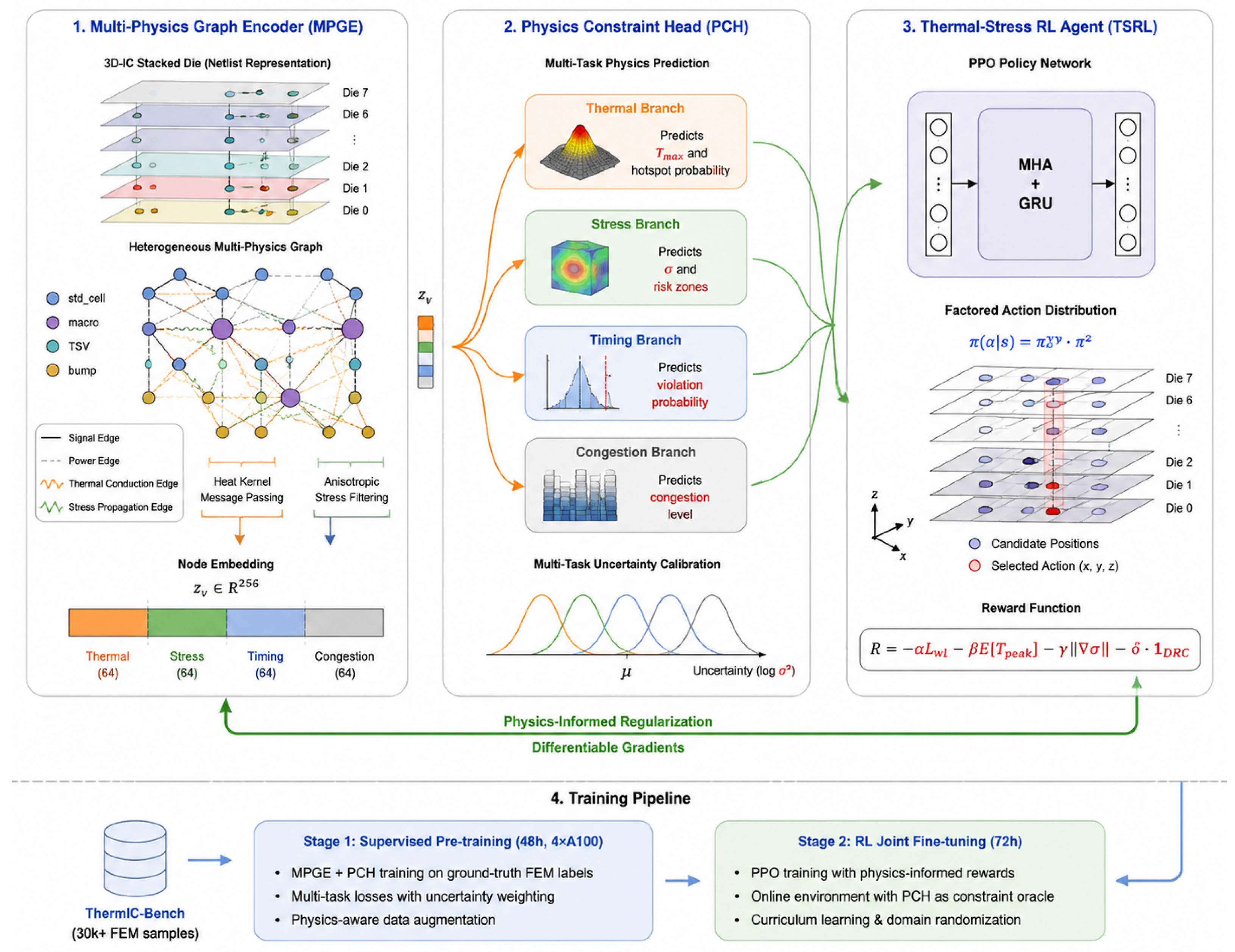
Figure 1.
Overall architecture of the ThermIC framework, including the MPGE graph encoder, the PCH constraint-prediction module, and the TSRL placement agent. The information flow is from the heterogeneous 3D netlist and material attributes to local physical-risk estimates and then to sequential placement decisions.
Figure 1.
Overall architecture of the ThermIC framework, including the MPGE graph encoder, the PCH constraint-prediction module, and the TSRL placement agent. The information flow is from the heterogeneous 3D netlist and material attributes to local physical-risk estimates and then to sequential placement decisions.
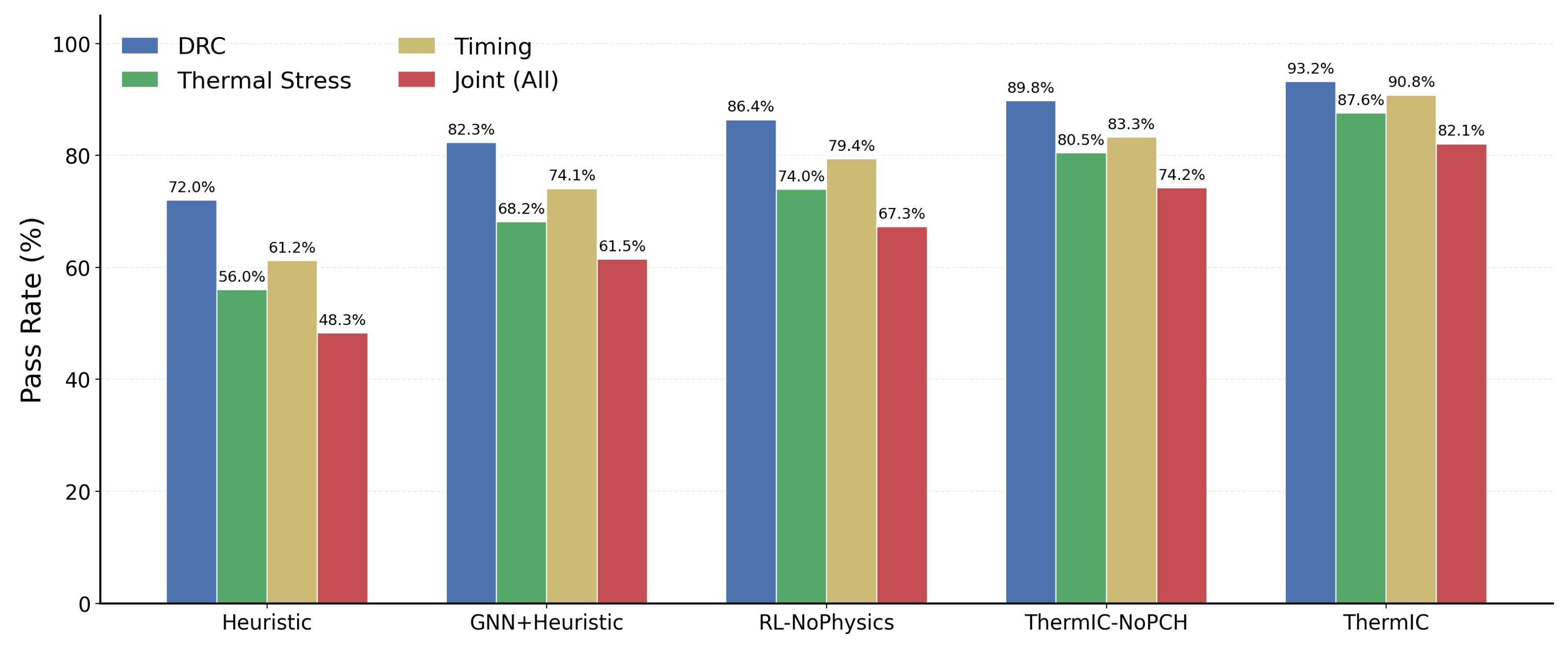
Figure 2.
The physical verification pass rate of each method is divided into DRC, thermo-mechanical stress, timing and joint pass categories.
Figure 2.
The physical verification pass rate of each method is divided into DRC, thermo-mechanical stress, timing and joint pass categories.
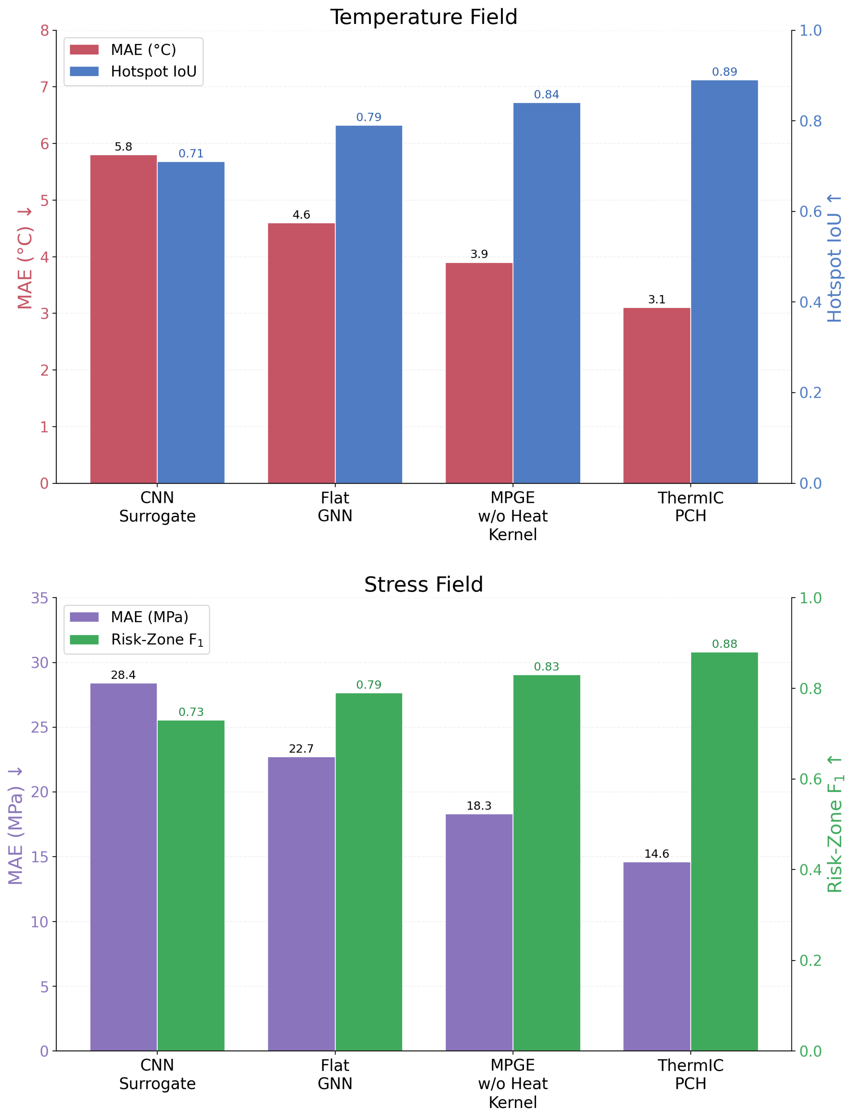
Figure 3.
Prediction accuracy comparison for the temperature field and thermo-mechanical stress field (MAE and IoU/ metrics) across four methods: CNN surrogate, flat GNN, MPGE without heat kernel, and full ThermIC PCH.
Figure 3.
Prediction accuracy comparison for the temperature field and thermo-mechanical stress field (MAE and IoU/ metrics) across four methods: CNN surrogate, flat GNN, MPGE without heat kernel, and full ThermIC PCH.
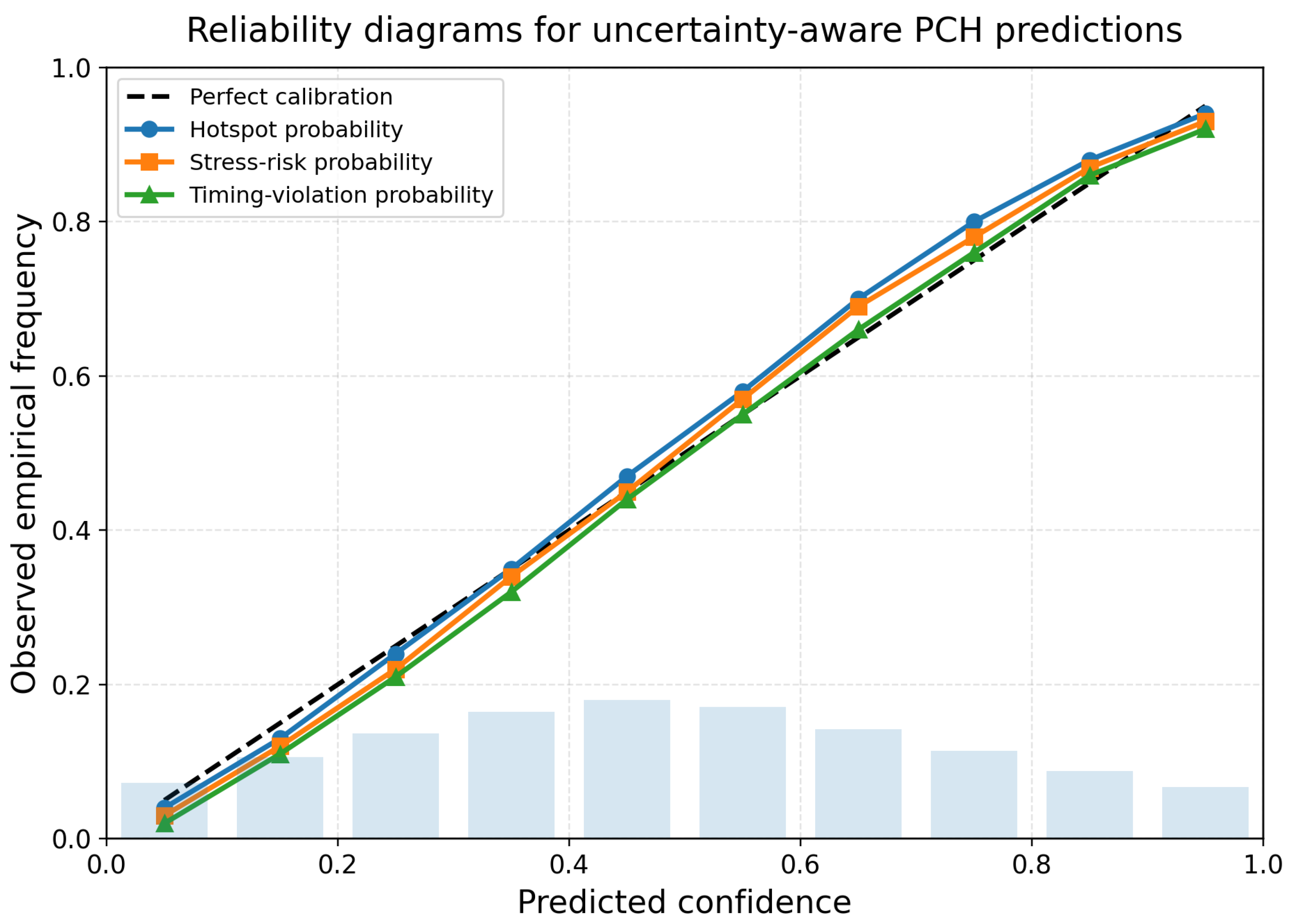
Figure 4.
Reliability diagrams for uncertainty-aware PCH predictions on the held-out test set. The diagonal line indicates perfect calibration; curves closer to the diagonal indicate better agreement between predicted confidence and empirical event frequency.
Figure 4.
Reliability diagrams for uncertainty-aware PCH predictions on the held-out test set. The diagonal line indicates perfect calibration; curves closer to the diagonal indicate better agreement between predicted confidence and empirical event frequency.
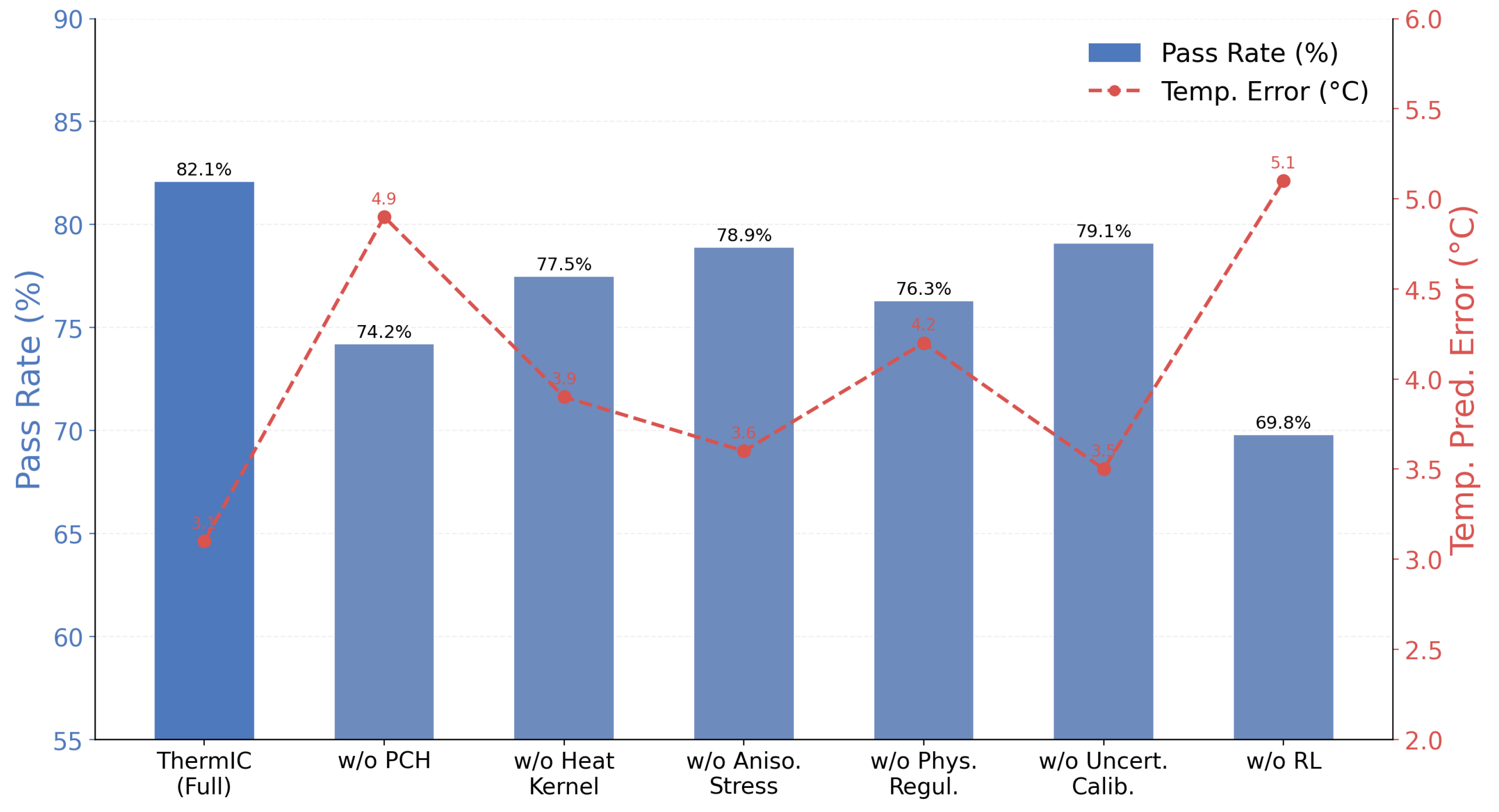
Figure 5.
Overall ablation study of ThermIC. Bars indicate physical verification pass rate, and the line indicates peak-temperature error.
Figure 5.
Overall ablation study of ThermIC. Bars indicate physical verification pass rate, and the line indicates peak-temperature error.
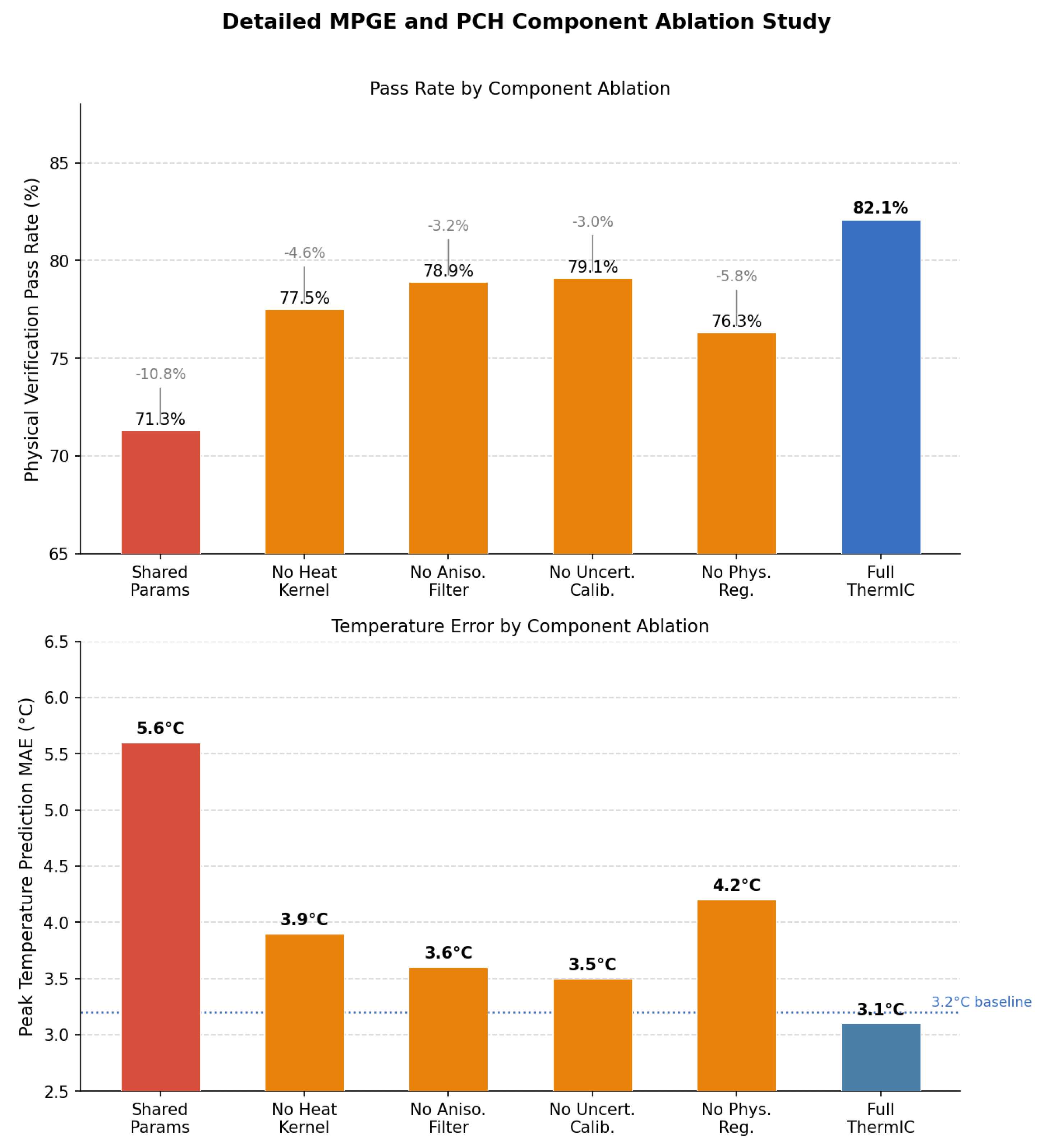
Figure 6.
Detailed MPGE and PCH component ablation across six configurations: shared-parameter edges (Shared Params), removal of heat kernel (No Heat Kernel), removal of anisotropic stress filtering (No Aniso. Filter), removal of uncertainty calibration (No Uncert. Calib.), removal of physics-informed regularization (No Phys. Reg.), and the full ThermIC model. Upper: physical verification pass rate; Lower: peak temperature prediction MAE. All ablated variants fall below the °C target line (dotted), consistent with the contribution of each component.
Figure 6.
Detailed MPGE and PCH component ablation across six configurations: shared-parameter edges (Shared Params), removal of heat kernel (No Heat Kernel), removal of anisotropic stress filtering (No Aniso. Filter), removal of uncertainty calibration (No Uncert. Calib.), removal of physics-informed regularization (No Phys. Reg.), and the full ThermIC model. Upper: physical verification pass rate; Lower: peak temperature prediction MAE. All ablated variants fall below the °C target line (dotted), consistent with the contribution of each component.
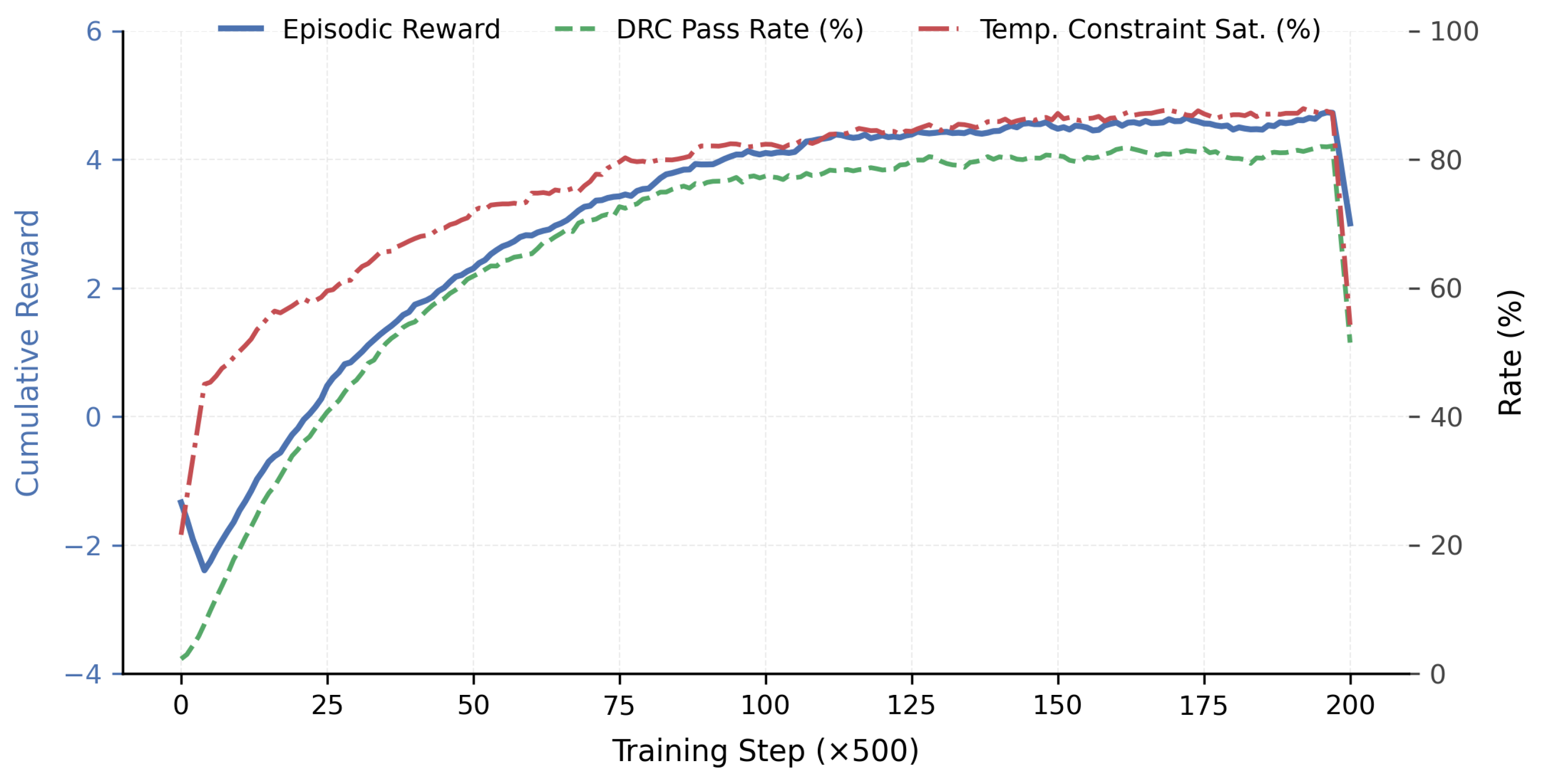
Figure 7.
Training curves of the TSRL agent during the RL joint fine-tuning stage, including cumulative reward, peak-temperature pass rate, and DRC pass rate.
Figure 7.
Training curves of the TSRL agent during the RL joint fine-tuning stage, including cumulative reward, peak-temperature pass rate, and DRC pass rate.
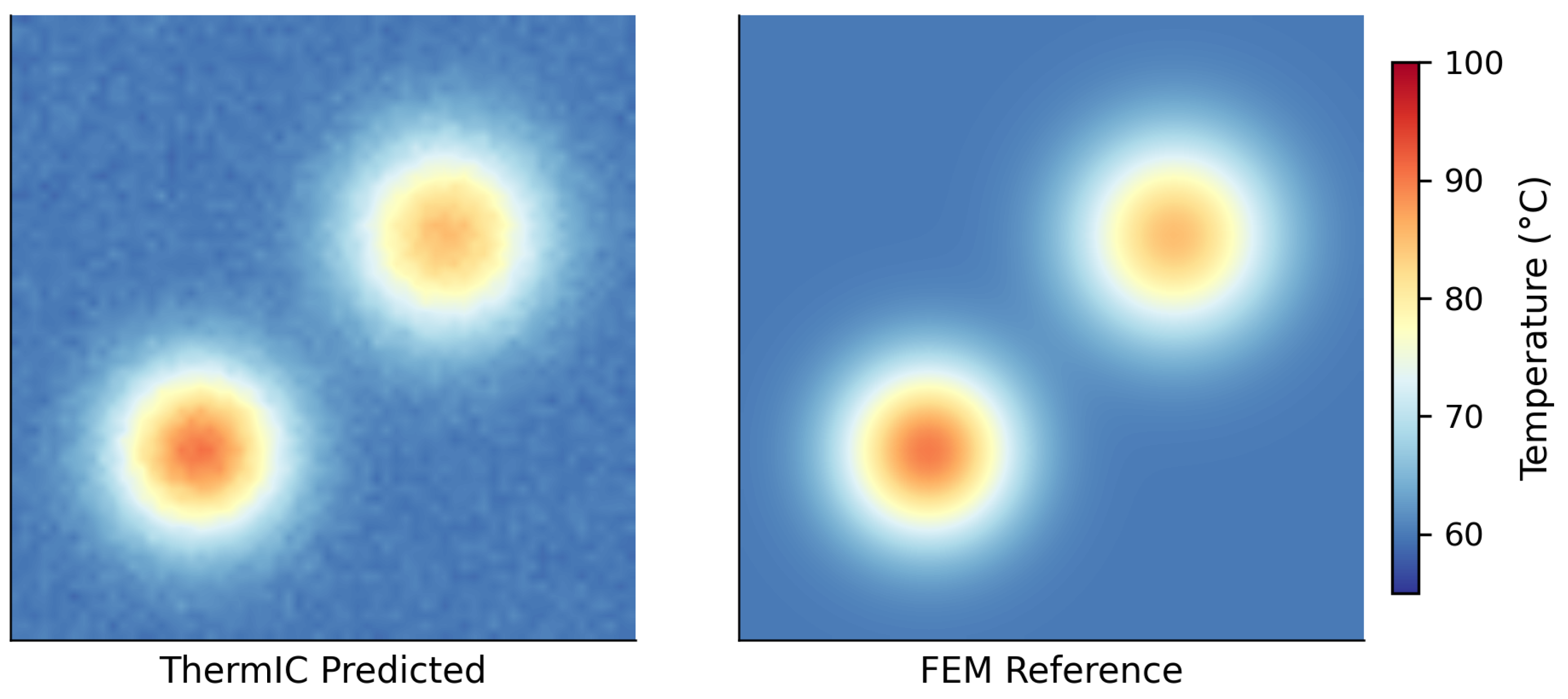
Figure 8.
Thermal map of interlayer temperature distribution. Left: PCH prediction; Right: COMSOL FEM reference.
Figure 8.
Thermal map of interlayer temperature distribution. Left: PCH prediction; Right: COMSOL FEM reference.
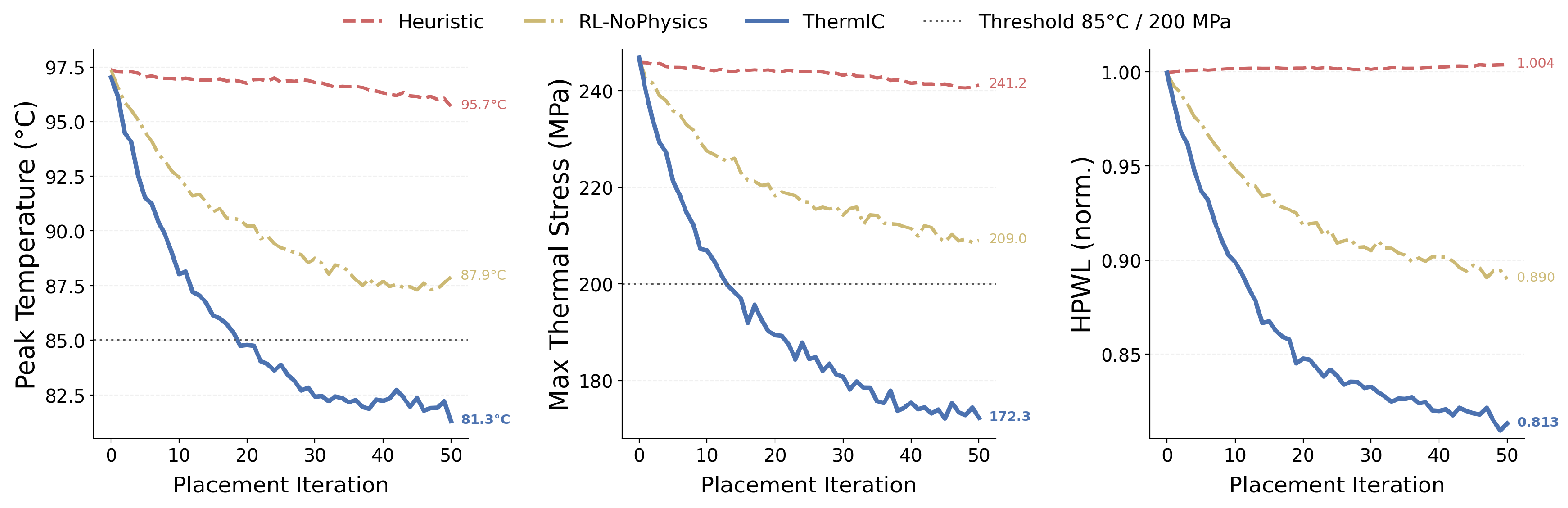
Figure 9.
Thermal–mechanical constraint optimization analysis on a representative 3D-IC design: evolution of peak temperature, maximum thermo-mechanical stress, and global wirelength throughout the optimization process for Heuristic, RL-NoPhysics, and full ThermIC.
Figure 9.
Thermal–mechanical constraint optimization analysis on a representative 3D-IC design: evolution of peak temperature, maximum thermo-mechanical stress, and global wirelength throughout the optimization process for Heuristic, RL-NoPhysics, and full ThermIC.
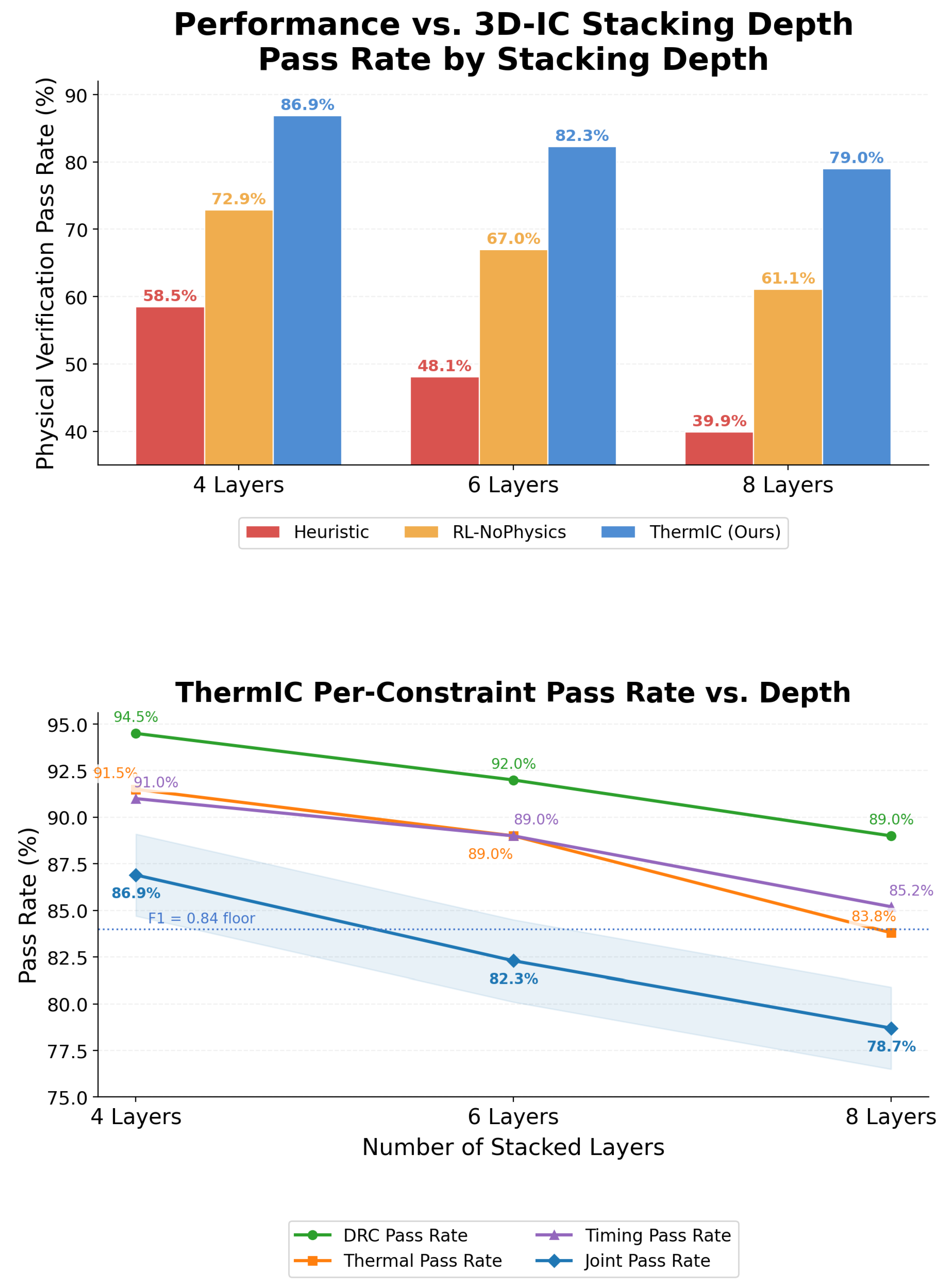
Figure 10.
ThermIC performance versus 3D-IC stacking depth. Upper: pass rate comparison of Heuristic, RL-NoPhysics, and ThermIC for 4-, 6-, and 8-tier designs. Lower: DRC, thermal, timing, and joint pass rate breakdown for ThermIC.
Figure 10.
ThermIC performance versus 3D-IC stacking depth. Upper: pass rate comparison of Heuristic, RL-NoPhysics, and ThermIC for 4-, 6-, and 8-tier designs. Lower: DRC, thermal, timing, and joint pass rate breakdown for ThermIC.
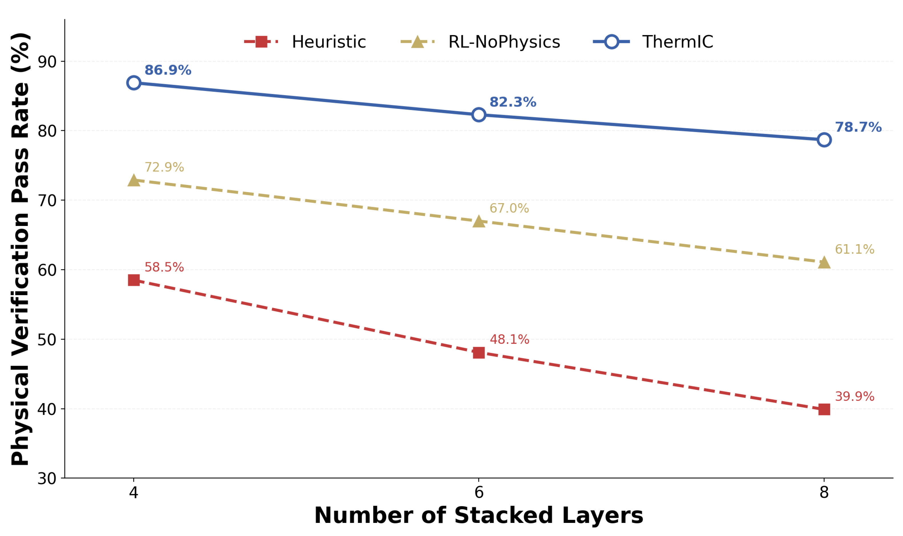
Figure 11.
Physical verification pass rate as a function of 3D-IC stacking depth for Heuristic, RL-NoPhysics, and ThermIC.
Figure 11.
Physical verification pass rate as a function of 3D-IC stacking depth for Heuristic, RL-NoPhysics, and ThermIC.
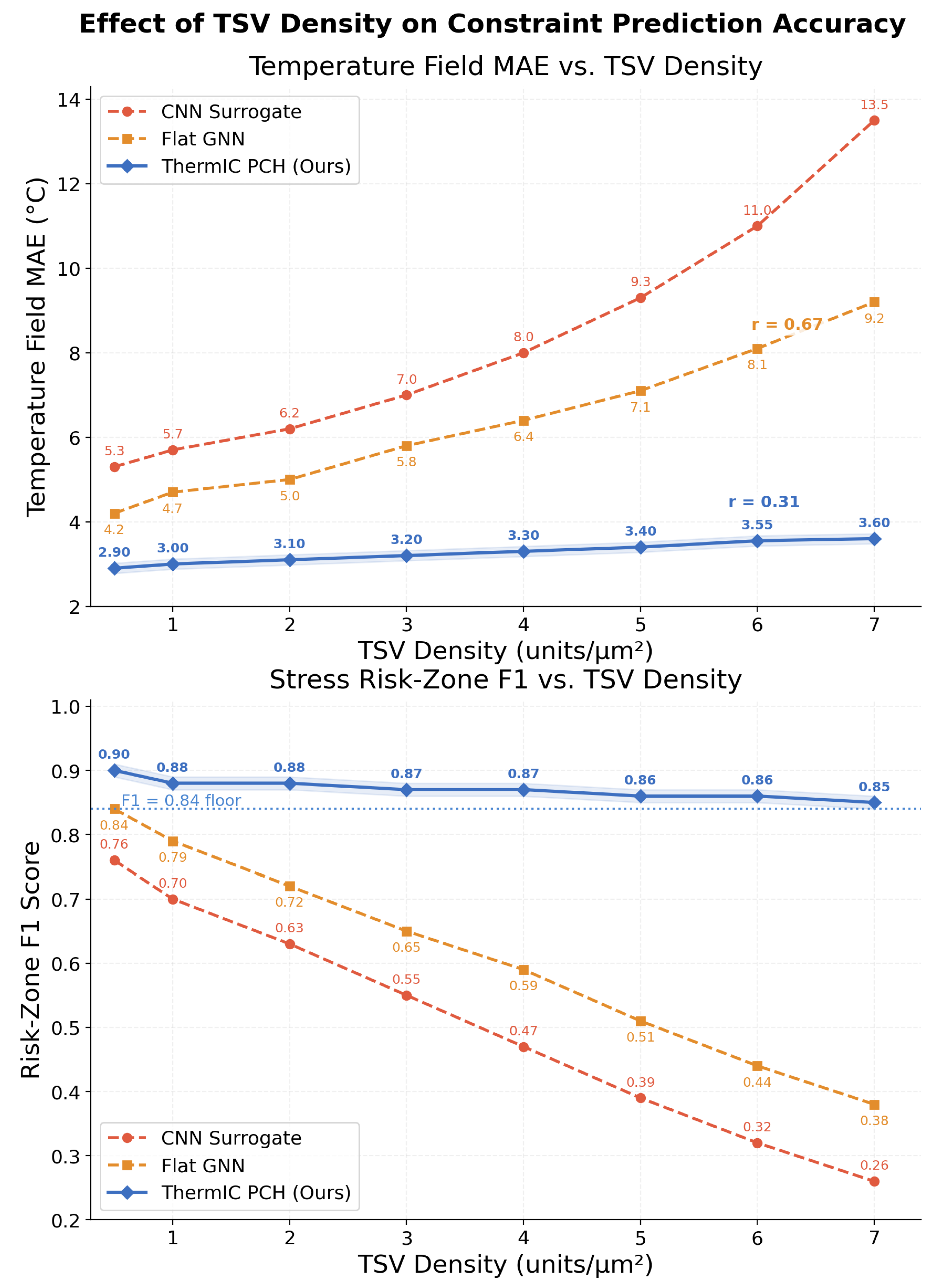
Figure 12.
Effect of TSV density on constraint prediction accuracy. Upper: temperature-field MAE versus TSV density for CNN Surrogate, Flat GNN, and ThermIC PCH. Lower: stress risk zone score for the same methods.
Figure 12.
Effect of TSV density on constraint prediction accuracy. Upper: temperature-field MAE versus TSV density for CNN Surrogate, Flat GNN, and ThermIC PCH. Lower: stress risk zone score for the same methods.
Figure 13.
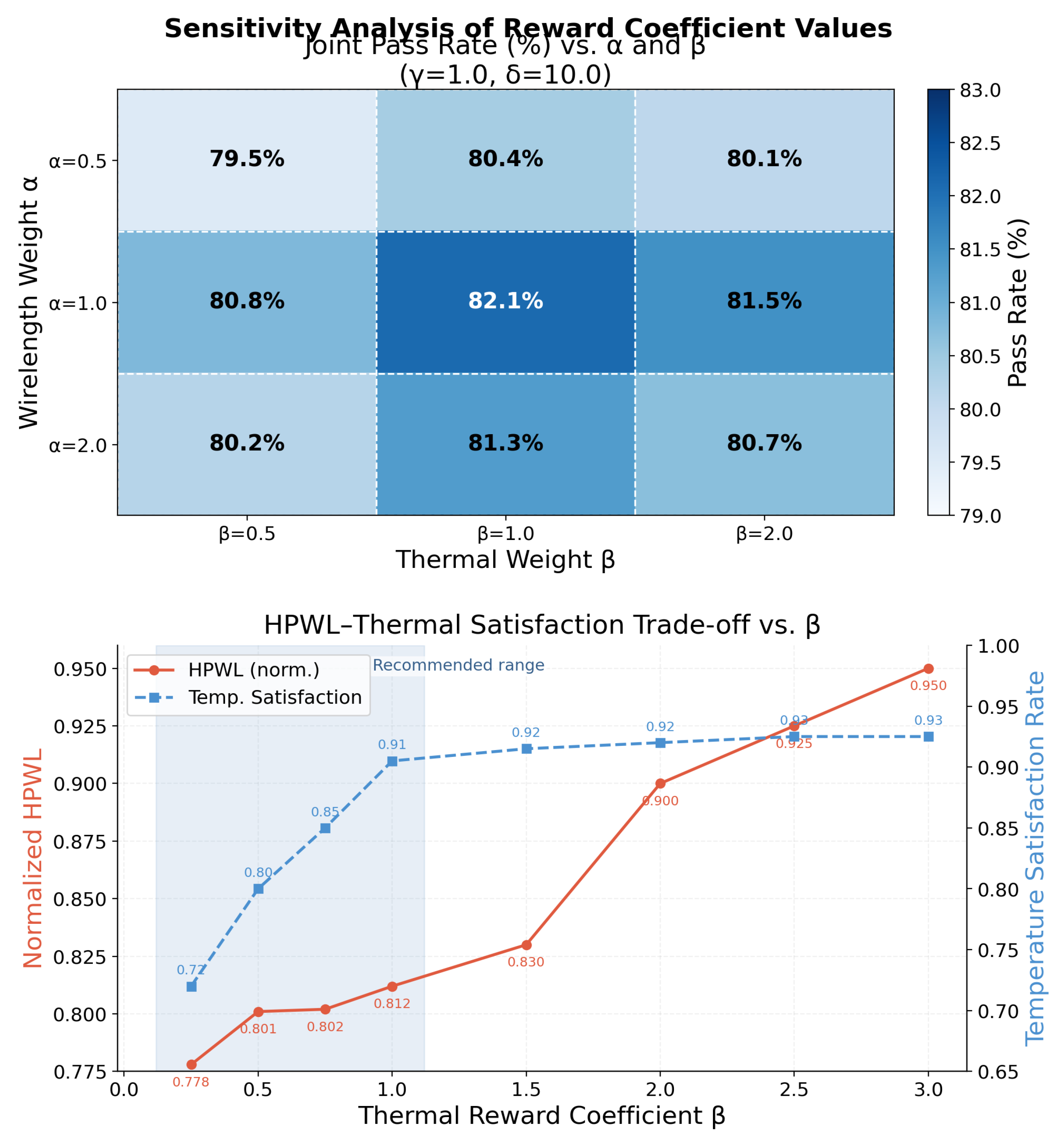
Sensitivity analysis of reward coefficient values. Upper: joint pass rate (%) heatmap over thermal weight and wirelength weight (, ); pass rates range only from to across the local 81-combination sweep, indicating local robustness around the Pareto-selected coefficient setting. Lower: trade-off between normalized HPWL and temperature satisfaction rate as varies; the shaded region marks the recommended coefficient range that simultaneously maintains HPWL and temperature satisfaction
Figure 13.
Sensitivity analysis of reward coefficient values. Upper: joint pass rate (%) heatmap over thermal weight and wirelength weight (, ); pass rates range only from to across the local 81-combination sweep, indicating local robustness around the Pareto-selected coefficient setting. Lower: trade-off between normalized HPWL and temperature satisfaction rate as varies; the shaded region marks the recommended coefficient range that simultaneously maintains HPWL and temperature satisfaction
Figure 14.
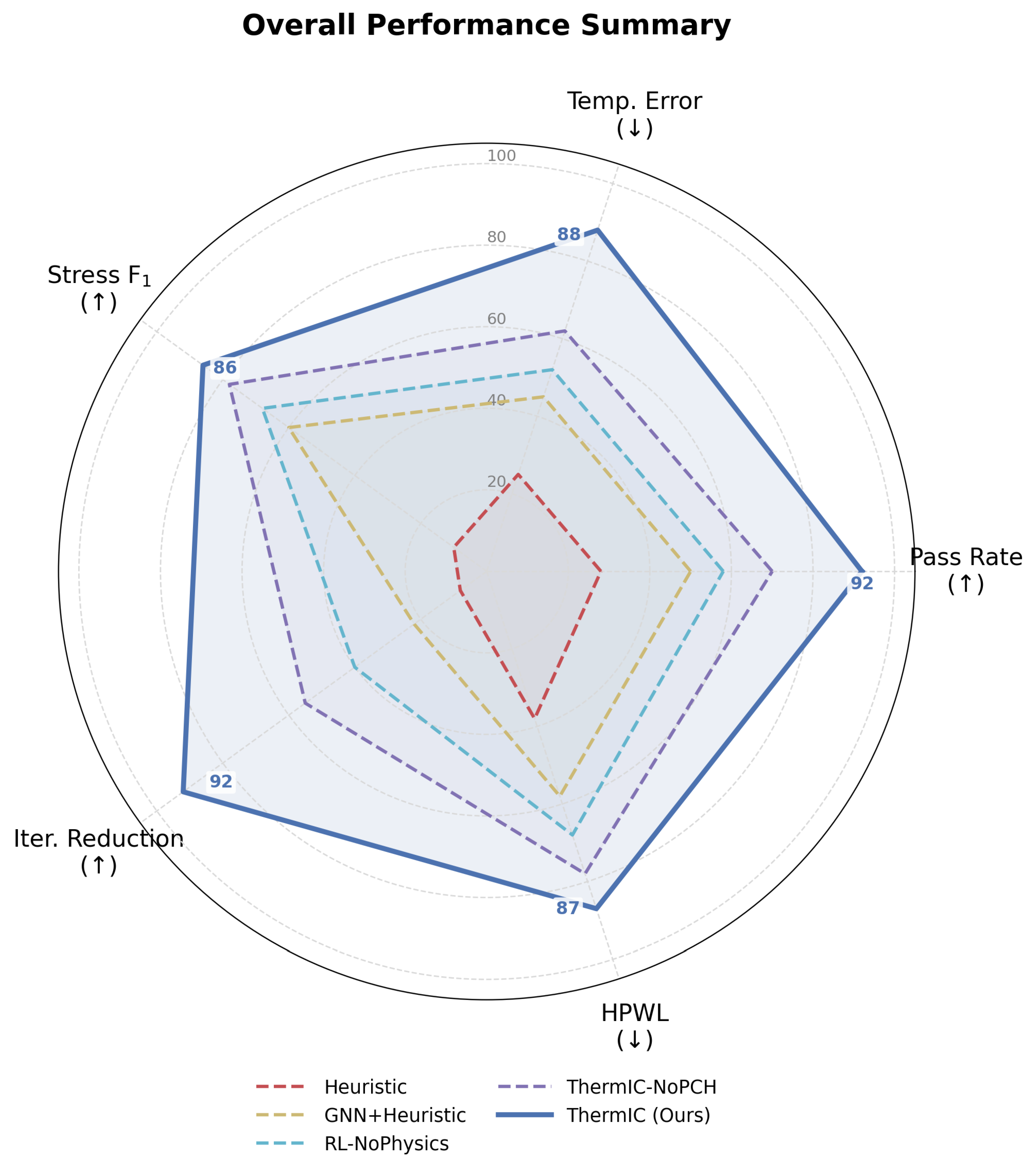
Overall performance summary radar chart across five dimensions: physical verification pass rate, temperature error (lower is better), stress prediction , design iteration reduction factor, and normalized wirelength.
Figure 14.
Overall performance summary radar chart across five dimensions: physical verification pass rate, temperature error (lower is better), stress prediction , design iteration reduction factor, and normalized wirelength.
Figure 15.
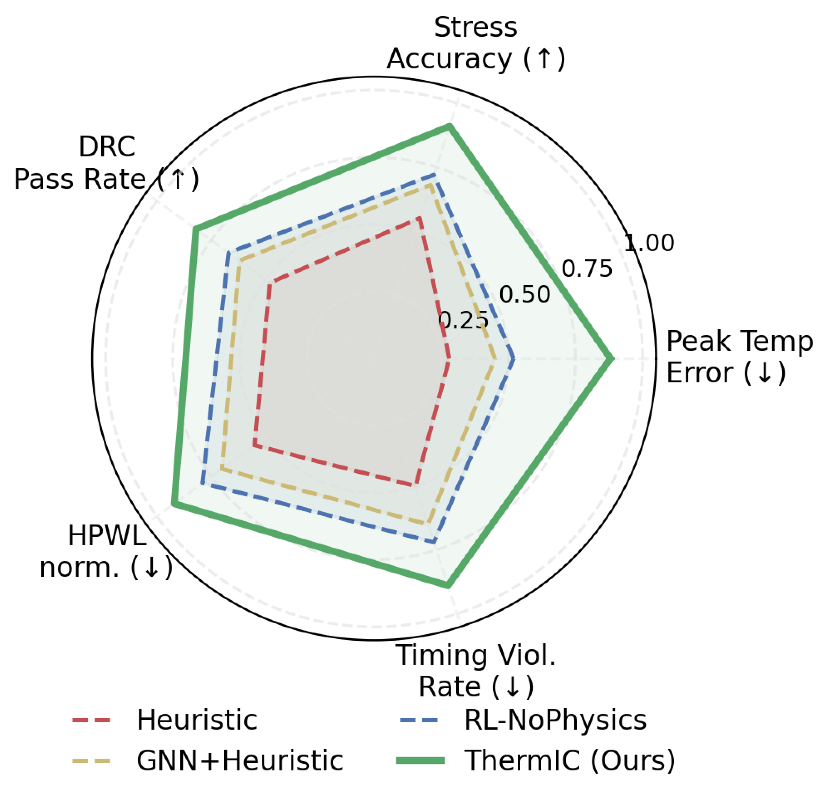
Radar chart comparing ThermIC and baseline methods across peak-temperature error, thermo-mechanical stress prediction accuracy, DRC pass rate, normalized wirelength, and timing violation rate.
Figure 15.
Radar chart comparing ThermIC and baseline methods across peak-temperature error, thermo-mechanical stress prediction accuracy, DRC pass rate, normalized wirelength, and timing violation rate.
Table 1.
Positioning of ThermIC relative to representative AI-driven placement frameworks.
Table 1.
Positioning of ThermIC relative to representative AI-driven placement frameworks.
| Framework | Main Learning Mechanism | Main Optimization Focus | Difference from ThermIC |
|---|
| Google RL placer [14] | Edge-based GCN with reinforcement learning | 2D macro placement and PPA-oriented floorplanning | ThermIC uses physically typed 3D graph channels and exposes thermal/stress risk to the policy at each placement step. |
| MaskPlace [15] | Reinforced visual representation learning | High-resolution 2D placement with wirelength, congestion, and density objectives | ThermIC does not rely on a purely visual canvas; it represents heat-flow and stress-propagation paths as graph relations in a stacked-die geometry. |
| DREAMPlace [16] | GPU-accelerated analytical placement formulated with deep-learning toolkits | Fast analytical global placement and legalization | ThermIC is not primarily an acceleration framework; it introduces differentiable multi-physics risk prediction as feedback for 3D placement decisions. |
| ChiPFormer [38] | Offline decision transformer for transferable placement | Transfer learning from fixed placement trajectories and few-shot fine-tuning on unseen 2D circuits | ThermIC shares the goal of transferable learned placement but differs by explicitly modeling coupled thermal–mechanical risk in 3D stacked layouts. |
| DREAMPlace 4.0 [39] | Timing-driven analytical placement with momentum-based net weighting | Timing-aware global and detailed placement | ThermIC considers timing jointly with thermal, stress, congestion, and DRC risks instead of optimizing timing as the primary differentiator. |
| AutoDMP [40] | DREAMPlace-based macro placement with automated multi-objective parameter tuning | Concurrent macro/cell placement and PPA-oriented exploration | ThermIC uses a learned physical-risk head as an online constraint oracle, whereas AutoDMP primarily improves macro-placement exploration and parameter tuning. |
| RoutePlacer [41] | Large-scale RouteGNN surrogate for routability-aware placement | End-to-end routability optimization and plug-in routing feedback | ThermIC uses graph prediction for thermal, stress, timing, congestion, and DRC risk in 3D-IC placement rather than routability alone. |
| TransPlace [42] | Transferable large-scale graph placement with netlist topology and position encoding | Generalizable global placement for millions of mixed-size cells | ThermIC targets stacked-die physical feasibility and uses explicitly typed heat-flow and stress-propagation edges. |
| ThermIC (this work) | Physics-typed heterogeneous graph encoding, uncertainty-aware constraint head, and thermal–stress RL policy | Joint DRC, thermal, stress, timing, and congestion-aware 3D-IC placement | The novelty is the closed-loop coupling of physical message passing, local risk prediction, and policy action selection for multi-tier layouts. |
Table 2.
Implementation-level ThermIC architecture, internal representation sizes, parameter counts, and graph-processing costs.
Table 2.
Implementation-level ThermIC architecture, internal representation sizes, parameter counts, and graph-processing costs.
| Stage | Internal Representation | Architectural Decision | Trainable Parameters | Dominant Processing Cost |
|---|
| Node/edge projection | ; edge attributes | Type-specific linear projections for standard cells, macros, TSVs, and bumps; edge features encode distance, tier gap, conductance proxy, CTE mismatch, stiffness contrast, and net degree | ∼0.32 M | |
| Relation-specific MPGE layer | with four 64-dimensional subspaces | Four edge-type operators for signal, power/current, thermal, and stress edges; residual connection, layer normalization, ReLU, and dropout after each layer | ∼0.56 M per layer; four layers ∼2.24 M | per layer |
| Heat-kernel thermal aggregation | Thermal subspace | Conductance-weighted graph heat kernel derived from the discrete heat equation; neighbor cap 32 for local thermal windows | ∼0.09 M | |
| Anisotropic stress filtering | Stress subspace | Direction-, CTE-, and stiffness-weighted stress filter separating vertical TSV-axis propagation from lateral in-plane propagation | ∼0.11 M | |
| PCH physical-risk heads | | Four independent two-layer MLP heads with width 128; uncertainty outputs for thermal and task weighting | ∼0.86–0.90 M | |
| TSRL actor–critic | Risk maps + partial placement state , , and | Four-head attention over candidate/placed nodes, GRU hidden size 256, actor and critic MLP width 128, factored 3D action distribution | ∼1.55–1.65 M | per decision step |
| Full ThermIC | MPGE + PCH + TSRL | End-to-end placement-time coupling between typed graph propagation, physical-risk prediction, and RL action selection | ∼5.2 M | Inference dominated by |
Table 3.
Default constraint thresholds used in ThermIC-Bench and their transferability.
Table 3.
Default constraint thresholds used in ThermIC-Bench and their transferability.
| Constraint | Default in this Study | Rationale in ThermIC-Bench | Transfer to Other Technologies |
|---|
| Peak temperature | °C
| Conservative hotspot boundary for the simulated stack; used to create near-threshold thermal-risk labels and to penalize excessive thermal accumulation. | Replace with the junction-temperature or package-level limit specified by the target PDK, product class, and reliability guardband. |
| Thermo-mechanical stress | from stack material limit | Determined by the weakest copper/inter-layer dielectric/bonding-interface limit in the simulated stack. | Recompute from process-specific material data, TSV geometry, bonding interface, and fatigue/yield criteria. |
| Timing slack | | Standard setup-time feasibility boundary after thermally derated timing analysis. | Replace with design-specific timing guardband, clock margin, or sign-off corner requirement. |
| DRC/LVS pass ratio | | Benchmark-level acceptance rule used to distinguish nearly legal placements from strongly violating layouts during early placement optimization. | For tape-out, replace with the sign-off rule deck requirement, normally complete DRC/LVS closure. |
Table 4.
Rationale for the relation-specific graph structure used by MPGE.
Table 4.
Rationale for the relation-specific graph structure used by MPGE.
| Relation Type | Physical/Design-Flow Rationale | Graph Construction Rule | Reason for Separation |
|---|
| Signal | Logical connectivity, wirelength, timing-path dependency, and fanout coupling | Netlist-derived cell–pin–net adjacency and critical-path membership | Messages mainly encode functional/timing dependency rather than spatial diffusion |
| Power/current | Switching-power concentration, local current demand, and IR-drop-prone neighborhoods | Power-grid neighborhood, estimated current adjacency, and power-density bins | Current demand affects heat generation and supply integrity but is not identical to signal connectivity |
| Thermal | Die-to-die heat conduction, TSV/micro-bump thermal paths, TIM resistance, and package boundary effects | Spatial thermal windows weighted by conductance proxies, layer gap, TSV proximity, and material attributes | Thermal diffusion follows distance- and conductance-dependent attenuation rather than netlist topology alone |
| Stress | CTE mismatch, stiffness contrast, TSV-induced stress concentration, and bonding-interface mechanical coupling | Anisotropic neighborhoods weighted by CTE difference, effective stiffness, vertical/lateral direction, and distance | Mechanical stress transfer is direction-dependent and should not be mixed with heat or timing messages |
Table 5.
Qualitative impact assessment of omitting explicit electromigration modelling from the current MPGE graph.
Table 5.
Qualitative impact assessment of omitting explicit electromigration modelling from the current MPGE graph.
| Potential EM-Related Case | Likely Error If EM Is Ignored | Possible Effect on Reported Results | Required Mitigation |
|---|
| High-current power-grid or TSV/bump neighborhood | Thermal risk may be captured, but local current crowding and via redundancy are not explicitly evaluated | Joint pass rate may overestimate reliability for EM-limited layouts | Post-route EM sign-off or current-density-labelled EM edge |
| Narrow long interconnect with moderate temperature | Placement may appear thermally safe while increasing current density along a critical wire segment | Potential EM false negatives not reflected in thermal/stress metrics | Line-width, duty-cycle, and current-density labels |
| Thermally hot but well-reinforced metal region | A simple current/temperature proxy may over-penalize a region with wide metal or redundant vias | Proxy EM relation may create false positives and unnecessary wirelength increase | Technology-aware EM labels rather than temperature-only proxies |
| Time-dependent material ageing | Static placement labels do not capture cumulative damage over operating history | Long-term lifetime risk remains outside the present benchmark evidence | Temperature-time, current-time, and stress-cycle reliability data |
Table 6.
Pareto-based selection procedure for the TSRL reward coefficients in Equation (
13).
Table 6.
Pareto-based selection procedure for the TSRL reward coefficients in Equation (
13).
| Step | Implementation Detail | Selection Criterion or Output |
|---|
| Candidate grid | ; | 81 reward settings evaluated on the held-out validation layouts |
| Validation objectives | Joint pass rate, normalized HPWL, thermal-violation margin, stress-gradient penalty, DRC failure rate | Objectives are normalized to avoid a single metric dominating due to scale |
| Pareto filtering | Discard settings dominated simultaneously in pass rate, HPWL, thermal/stress risk, and DRC failure | Produces a compact non-dominated set of candidate trade-offs |
| Knee-point selection | Compute distance from each non-dominated point to the normalized ideal point | Select |
| Test-set use | No coefficient tuning is performed on the test layouts | The selected coefficient vector is fixed before final evaluation |
Table 7.
Composition of the ThermIC-Bench dataset.
Table 7.
Composition of the ThermIC-Bench dataset.
| Data Type | Source | Scale | Key Features |
|---|
| OSS 3D-IC | Open3DIC/IWLS 2023 | 12 designs, 4–8 layers | TSV dist., thermal net |
| Industry-style | 3D-MCNC/ISPD derived, technology-mapped | 6 large designs | 10 k–200 k cells |
| Multi-Physics | Fluent + COMSOL | 2 k layouts/design | Temp., stress, timing |
Timing/
power | PrimeTime + RedHawk | Paired features | Path delay, IR-drop |
Table 8.
Computational complexity, memory requirement, and deployment interpretation of the main ThermIC stages.
Table 8.
Computational complexity, memory requirement, and deployment interpretation of the main ThermIC stages.
| Stage | Dominant Operation | Asymptotic Cost | Memory Driver | Deployment Interpretation |
|---|
| Graph construction | Build signal, power, thermal, and stress adjacency from layout objects | | Sparse edge lists and node attributes | Performed once per design snapshot and can be cached between placement iterations |
| MPGE–PCH inference | Relation-specific sparse message passing and multi-head risk prediction | | Node embeddings, edge indices, and activations | Main online overhead; no FEM solve is required during policy rollout |
| TSRL action scoring | Evaluate candidate 3D coordinates using policy logits and PCH risk fields | per placement step after candidate pruning | Candidate buffer and local risk maps | Cost is controlled by limiting candidates to legal bins and high-risk neighborhoods |
| Offline FEM labeling | Thermal CFD, structural mechanics, timing, and IR-drop sign-off labels | Tool- and mesh-dependent; approximately 150,000 CPU-core-hours in this study | Simulation mesh and field outputs | One-time benchmark-generation cost; not repeated for every deployment run |
| Two-stage training | Supervised MPGE–PCH pre-training and RL fine-tuning | Approximately 48 h + 72 h on 4 × A100 for this study | Training activations, replay buffer, optimizer states | Amortized offline cost; practical users can start from released checkpoints and fine-tune selectively |
Table 9.
Real-world relevance assessment and current validation boundary of ThermIC.
Table 9.
Real-world relevance assessment and current validation boundary of ThermIC.
| Evidence Layer | Validation Evidence | Supported Interpretation | Remaining Limitation |
|---|
| Benchmark scope | Simulation-based ThermIC-Bench validation without tape-out or silicon measurements | Prevents over-claiming of industrial deployment readiness | No measured thermal/stress data are available |
| Public EDA interface | Inputs mapped to cells, nets, bins, tiers, TSVs, power maps, and LEF/DEF-like geometry | The model can be connected to standard physical-design artifacts | PDK- and sign-off-deck-specific adaptation is still required |
| Open benchmark relevance | Data abstraction aligned with CircuitNet, CircuitNet 2.0, and Open3DBench | Shows compatibility with public ML-for-EDA and 3D-IC benchmark directions | Most public datasets lack coupled 3D thermal–stress labels |
| Industrial applicability | Pre-signoff placement-assistant role aimed at reducing late correction cycles | Supports practical workflow relevance under simulated sign-off checks | Foundry NDA circuits, package-specific calibration, and tape-out studies remain future work |
Table 10.
Adaptation, hyperparameter tuning, and equal-comparison protocol for modern AI-based placement baselines on ThermIC-Bench.
Table 10.
Adaptation, hyperparameter tuning, and equal-comparison protocol for modern AI-based placement baselines on ThermIC-Bench.
| Protocol Item | Adaptation Applied to RoutePlacer/TransPlace and Other Modern Baselines | Equal-Comparison Control | Purpose |
|---|
| Input conversion | LEF/DEF-like geometry, netlist, macro, bin, tier, TSV, power-density, and density-map features are converted into each method’s required graph or placement-grid format. For methods that expect 2D inputs, each tier is treated as a legal placement layer with inter-tier TSV features appended as additional node/edge attributes. | All methods receive the same training, validation, and test designs and the same placement legality masks; PCH risk fields are not provided to external baselines. | Prevents feature leakage from ThermIC’s physical-risk predictor. |
| 3D legalization | Outputs from 2D or macro-placement methods are mapped to legal 3D coordinates by a common tier-assignment and overlap-removal legalization step that respects fixed macros, TSV keep-out zones, density limits, and tier capacities. | The same legalization code and failure-handling rules are used for DREAMPlace 4.0, Google RL, MaskPlace, ChiPFormer, AutoDMP, RoutePlacer, and TransPlace. | Ensures that differences do not arise from method-specific legalizers. |
| RoutePlacer adaptation | The RouteGNN/routability surrogate is trained on the ThermIC-Bench training split using netlist, bin-density, and congestion features; its routability objective is retained, while tier assignment and thermal–stress verification are added only as external evaluation steps. | Validation tuning uses the same candidate learning rates, batch sizes, early-stopping rule, and rollout budget as other learned baselines. | Tests whether routability-aware graph placement transfers to 3D multi-physics evaluation. |
| TransPlace adaptation | The transferable graph-placement encoder is trained with ThermIC-Bench topology and position encodings; 3D tier IDs and TSV-neighborhood features are appended, but the method is not given ThermIC’s heat-kernel, stress-filter, or PCH outputs. | The same validation split selects hidden width, number of graph layers, learning rate, dropout, and placement-temperature parameters. | Tests a modern transferable large-scale graph placer under the same 3D legality constraints. |
| Hyperparameter tuning | Each learned baseline is tuned over a shared validation budget of 20 configurations, covering learning rate, hidden dimension, graph depth, dropout, placement penalty weights, and legalization penalty strength where applicable. | No test-layout labels or test-set physical-verification outcomes are used for tuning. The best checkpoint is selected by validation HPWL plus legality plus joint-verification proxy. | Avoids giving ThermIC or any baseline a larger tuning budget. |
| Evaluation backend | After placement, every method is evaluated by the same DRC, thermal, stress, timing, congestion, and joint-pass pipeline. | All reported metrics in Table 14 use the same threshold vector and the same held-out test layouts. | Makes Table 14 a comparison of resulting layouts, not of different sign-off flows. |
Table 11.
Reproducibility-oriented architecture specification of ThermIC.
Table 11.
Reproducibility-oriented architecture specification of ThermIC.
| Component | Input and Output | Architecture Setting | Key Hyperparameters | Approx. Parameters |
|---|
| Graph construction | Standard cells, macros, TSVs, bumps, nets, tiers, power maps, and material attributes → heterogeneous graph | Four edge groups: signal, power/current, thermal-conduction, and stress-propagation edges; spatial windows are used for thermal and stress neighborhoods | Node features: geometry, power, timing slack, tier index, material ID, local density; edge features: distance, layer gap, conductance proxy, CTE/stiffness mismatch | Non-trainable preprocessing |
| MPGE encoder | Heterogeneous graph | Four relation-specific message-passing layers; each layer contains relation-specific linear projection, heat-kernel aggregation, anisotropic stress filter, residual connection, layer normalization, and ReLU | Hidden dimension 256; four 64-dimensional physical subspaces; dropout 0.10; neighbor cap 32 for thermal/stress windows | ∼2.7 M |
| PCH decoder | Node embedding and local graph state → physical-risk fields | Four two-layer MLP heads for thermal, stress, timing, and congestion prediction; each head uses shared MPGE embeddings but independent output layers | MLP width 128; homoscedastic uncertainty weighting; sigmoid output for violation probability; regression heads for and stress | ∼0.9 M |
| TSRL policy | PCH risk fields and placement state → factored action distribution | Multi-head attention over placed/unplaced nodes followed by GRU state update; actor predicts and ; critic estimates state value | 4 attention heads; GRU hidden size 256; actor/critic MLP width 128; candidate pruning by legal bins and risk neighborhoods | ∼1.6 M |
| Total model | MPGE + PCH + TSRL | End-to-end differentiable risk-guided placement policy | Mixed precision can be used for inference; lower MPGE layers can be frozen for fine-tuning | ∼5.2 M |
Table 12.
Training, hyperparameter, and benchmark-generation protocol used for reproducibility.
Table 12.
Training, hyperparameter, and benchmark-generation protocol used for reproducibility.
| Item | Setting Used in This Study | Reproducibility Note |
|---|
| Software and hardware | Python 3.10, PyTorch 2.x, CUDA-enabled training, 4×NVIDIA A100 GPUs for reported training runs | Code, configuration files, random seeds, and model checkpoints are intended to be released with the benchmark package |
| Data split | Design-level split with no layout variant shared across training, validation, and test partitions; validation set used for early stopping and Pareto coefficient selection | Prevents leakage from nearly identical placement variants and supports cross-design evaluation |
| Calibration split | A calibration-only subset of 600 layouts is held out from supervised training and PPO fine-tuning; it is disjoint from the final test designs and is used only for post-hoc calibration of PCH probabilities and predictive variances | Separates calibration from final evaluation and prevents the reliability diagrams, ECE, NLL, Brier score, PICP, and MPIW values from being fitted on the test set |
| Benchmark generation | Convert physical-design objects into graph nodes/edges; sample placement perturbations by Latin hypercube sampling; filter illegal initial layouts; generate 2000 variants per design around feasible and near-boundary layouts | Sampling is biased toward thermal, stress, timing, and DRC boundary cases so that the model learns constraint margins rather than only easy passing layouts |
| Label generation | Thermal CFD/finite-volume labels, COMSOL thermo-mechanical stress labels, PrimeTime thermally derated timing labels, and RedHawk IR-drop features | FEM/CFD labels are used offline for supervision and selected validation, not inside every online RL action step |
| Feature normalization | Continuous node, edge, and field features are standardized by training-set statistics; categorical material and layer IDs are embedded | The same training-set statistics are stored and reused at validation, test, and deployment time |
| Stage 1 pre-training | AdamW optimizer; learning rate ; weight decay ; batch size 32 graphs; gradient clipping 1.0; cosine decay; early stopping on validation physical-risk loss | MPGE and PCH are trained with uncertainty-weighted multi-task losses before RL exploration starts |
| Stage 2 RL fine-tuning | PPO-style policy update; policy learning rate ; value learning rate ; clip ratio 0.20; discount factor 0.99; GAE ; entropy coefficient 0.01; value-loss coefficient 0.5 | Lower MPGE layers are frozen; upper MPGE layers, PCH heads, actor, and critic are fine-tuned with risk-aware rewards |
| Reward coefficients | Pareto-selected default , with grid-based sensitivity analysis reported separately | The selected coefficients are fixed after validation and are not tuned on the test layouts |
| Randomness control | Three independent seeds are used for model initialization, data-loader order, and policy rollouts; reported values use the same held-out test split | This reduces dependence on a single favorable RL rollout and supports future replication |
| Checkpointing and evaluation | Best checkpoint selected by validation joint-pass proxy; final metrics computed once on the held-out test designs using the full verification pipeline | Test labels are not used for model selection or reward-coefficient tuning |
Table 13.
Physical verification pass rate comparison on ThermIC-Bench.
Table 13.
Physical verification pass rate comparison on ThermIC-Bench.
| Method | Pass Rate (%) | HPWL (Norm.) | Iterations | Temp. Error (°C) |
|---|
| Heuristic | 48.3 | 1.00 | 1.00× | 8.7 |
| GNN+Heuristic | 61.7 | 0.92 | 0.78× | 6.2 |
| RL-NoPhysics | 67.4 | 0.88 | 0.64× | 5.8 |
| ThermIC-NoPCH | 74.2 | 0.83 | 0.49× | 4.9 |
| ThermIC (Ours) | 82.1 | 0.81 | 0.27× | 3.1 |
Table 14.
Expanded comparison with recent AI-based and learning-assisted placement frameworks under the shared ThermIC-Bench evaluation protocol.
Table 14.
Expanded comparison with recent AI-based and learning-assisted placement frameworks under the shared ThermIC-Bench evaluation protocol.
| Method | Adaptation to ThermIC-Bench | Joint Pass (%) | HPWL (Norm.) | Temp. Error (°C) | Stress | Iterations |
|---|
| Heuristic thermal-aware placer [5,21] | Simulated annealing with compact thermal penalty | 48.3 | 1.00 | 8.7 | 0.61 | 1.00× |
| DREAMPlace 4.0-adapted [16,39] | GPU analytical/timing-driven placement followed by 3D tier legalization and post-placement multi-physics checking | 66.5 | 0.84 | 5.3 | 0.73 | 0.56× |
| Google RL placer-adapted [14] | Graph-based macro-placement policy with added tier legalization and identical post-placement verification | 70.8 | 0.86 | 5.1 | 0.75 | 0.50× |
| MaskPlace-adapted [15] | Reinforced visual placement with 3D legalization and common thermal–stress evaluation | 72.6 | 0.85 | 4.8 | 0.77 | 0.47× |
| ChiPFormer-adapted [38] | Offline decision-transformer policy fine-tuned on ThermIC-Bench trajectories without PCH risk feedback | 75.1 | 0.83 | 4.5 | 0.79 | 0.43× |
| AutoDMP-adapted [40] | Automated DREAMPlace-based macro/cell placement with multi-objective parameter tuning and shared verification | 73.4 | 0.82 | 4.7 | 0.78 | 0.45× |
| RoutePlacer-adapted [41] | Large-scale RouteGNN routability surrogate adapted to tier-aware placement and common thermal–stress verification | 74.4 | 0.84 | 4.6 | 0.80 | 0.42× |
| TransPlace-adapted [42] | Transferable graph-based global placement with netlist/position encoding, followed by 3D legalization and shared verification | 76.2 | 0.82 | 4.3 | 0.81 | 0.40× |
| ThermIC (ours) | Physics-typed graph encoding, uncertainty-aware physical-risk prediction, and thermal–stress RL feedback | 82.1 | 0.81 | 3.1 | 0.88 | 0.27× |
Table 15.
Physical verification pass rate and runtime comparison across design scales (cell count).
Table 15.
Physical verification pass rate and runtime comparison across design scales (cell count).
| Design ID | Layers | Cells (k) | TSVs (k) | Heuristic | RL-NoPhysics | ThermIC (Ours) |
|---|
|
Pass (%)
|
WL
|
Err. (°C)
|
Time (h)
|
Pass (%)
|
WL
|
Err. (°C)
|
Time (h)
|
Pass (%)
|
WL
|
Err. (°C)
|
|---|
| D1 | 4 | 10 | 2.1 | 61.2 | 1.00 | 7.8 | 2.1 | 74.5 | 0.91 | 5.4 | 3.8 | 88.3 | 0.83 | 2.9 |
| D2 | 4 | 25 | 5.3 | 55.8 | 1.00 | 8.2 | 4.5 | 71.3 | 0.89 | 5.8 | 7.4 | 85.6 | 0.82 | 3.2 |
| D3 | 6 | 50 | 11.7 | 50.4 | 1.00 | 8.9 | 9.2 | 68.1 | 0.87 | 6.1 | 15.7 | 83.4 | 0.80 | 3.4 |
| D4 | 6 | 100 | 22.4 | 45.7 | 1.00 | 9.4 | 18.6 | 65.8 | 0.86 | 6.4 | 31.2 | 81.2 | 0.81 | 3.6 |
| D5 | 8 | 150 | 34.6 | 41.2 | 1.00 | 10.1 | 27.3 | 62.4 | 0.88 | 6.8 | 46.8 | 79.5 | 0.82 | 3.8 |
| D6 | 8 | 200 | 45.2 | 38.5 | 1.00 | 10.8 | 37.1 | 59.7 | 0.89 | 7.2 | 62.5 | 77.8 | 0.83 | 4.1 |
Table 16.
Runtime and memory scaling of ThermIC during design-time inference. Forward time is measured for one MPGE–PCH evaluation; full placement time includes sequential TSRL rollout and legality checking.
Table 16.
Runtime and memory scaling of ThermIC during design-time inference. Forward time is measured for one MPGE–PCH evaluation; full placement time includes sequential TSRL rollout and legality checking.
| Design | Cells (k) | Edges (M) | MPGE–PCH Forward (ms) | RL-NoPhysics Time (h) | ThermIC Time (h) | Peak GPU Memory (GB) |
|---|
| D1 | 10 | 0.58 | 21 | 3.8 | 4.0 | 3.1 |
| D2 | 25 | 1.42 | 46 | 7.4 | 7.8 | 4.8 |
| D3 | 50 | 3.03 | 91 | 15.7 | 16.5 | 7.4 |
| D4 | 100 | 6.18 | 177 | 31.2 | 32.8 | 11.6 |
| D5 | 150 | 9.72 | 261 | 46.8 | 49.2 | 15.9 |
| D6 | 200 | 13.04 | 340 | 62.5 | 65.7 | 20.7 |
Table 17.
Measured training, inference, memory, and rollout-cost profiling for ThermIC and baseline methods. Latency is measured per policy/risk update on the evaluated graph; rollout time is measured for a complete placement episode.
Table 17.
Measured training, inference, memory, and rollout-cost profiling for ThermIC and baseline methods. Latency is measured per policy/risk update on the evaluated graph; rollout time is measured for a complete placement episode.
| Design | Method | Offline Training or Tuning (h) | Policy/Risk Update Latency (ms) | Full Rollout Time (h) | Peak GPU Memory (GB) | Relative Rollout Cost |
|---|
| D1 (10 k cells) | Heuristic | 0.0 | 12 | 2.1 | CPU-only | 0.53× |
| D1 (10 k cells) | RL-NoPhysics | 54.6 | 17 | 3.8 | 2.4 | 0.95× |
| D1 (10 k cells) | ThermIC | 120.3 | 21 | 4.0 | 3.1 | 1.00× |
| D3 (50 k cells) | Heuristic | 0.0 | 47 | 9.2 | CPU-only | 0.56× |
| D3 (50 k cells) | RL-NoPhysics | 54.6 | 82 | 15.7 | 5.8 | 0.95× |
| D3 (50 k cells) | ThermIC | 120.3 | 91 | 16.5 | 7.4 | 1.00× |
| D6 (200 k cells) | Heuristic | 0.0 | 186 | 37.1 | CPU-only | 0.56× |
| D6 (200 k cells) | RL-NoPhysics | 54.6 | 316 | 62.5 | 17.9 | 0.95× |
| D6 (200 k cells) | ThermIC | 120.3 | 340 | 65.7 | 20.7 | 1.00× |
Table 18.
Calibration quality of PCH probabilistic predictions. ECE and MCE are reported in percentage points. Lower ECE, MCE, NLL, Brier score, and CRPS are better; PICP should be close to the nominal 90% level.
Table 18.
Calibration quality of PCH probabilistic predictions. ECE and MCE are reported in percentage points. Lower ECE, MCE, NLL, Brier score, and CRPS are better; PICP should be close to the nominal 90% level.
| Prediction Target | Model/Output Variant | ECE/Miscal. (%) | MCE (%) | NLL | Brier/CRPS | PICP@90% |
|---|
| Hotspot probability | Uncalibrated PCH logits | 7.8 | 18.4 | 0.302 | 0.083 | – |
| Hotspot probability | ThermIC calibrated PCH (temperature scaling) | 2.6 | 7.1 | 0.241 | 0.062 | – |
| Stress-risk probability | Uncalibrated PCH logits | 8.4 | 19.7 | 0.331 | 0.092 | – |
| Stress-risk probability | ThermIC calibrated PCH (temperature scaling) | 2.9 | 7.8 | 0.267 | 0.071 | – |
| Timing-violation probability | Uncalibrated PCH logits | 6.5 | 15.9 | 0.256 | 0.067 | – |
| Timing-violation probability | ThermIC calibrated PCH (temperature scaling) | 2.4 | 6.5 | 0.198 | 0.052 | – |
| Thermal regression interval | ThermIC Gaussian uncertainty (variance scaling) | 3.8 | – | 1.74 | 1.22 °C | 88.7 |
| Stress regression interval | ThermIC Gaussian uncertainty (variance scaling) | 4.5 | – | 2.06 | 6.9 MPa | 87.9 |
Table 19.
Mechanism-level validation of the heat-kernel and anisotropic-stress modules on held-out ThermIC-Bench layouts. Lower heat residual and lower location error are better; higher gradient correlation and TSV-window are better.
Table 19.
Mechanism-level validation of the heat-kernel and anisotropic-stress modules on held-out ThermIC-Bench layouts. Lower heat residual and lower location error are better; higher gradient correlation and TSV-window are better.
| Model Variant | Heat Residual | Thermal-Gradient Corr. | TSV-Window Stress | Stress Peak Loc. Error (m) |
|---|
| Flat GNN surrogate | 0.182 | 0.74 | 0.71 | 15.6 |
| MPGE w/o heat kernel | 0.137 | 0.82 | 0.80 | 11.9 |
| MPGE w/o anisotropic stress filter | 0.091 | 0.89 | 0.76 | 13.4 |
| ThermIC PCH (full) | 0.083 | 0.91 | 0.86 | 7.4 |
Table 20.
Sensitivity of ThermIC to relation-type selection in the heterogeneous graph. “EM/degradation proxy” is an exploratory current-density/temperature-history proxy and is not interpreted as sign-off electromigration validation.
Table 20.
Sensitivity of ThermIC to relation-type selection in the heterogeneous graph. “EM/degradation proxy” is an exploratory current-density/temperature-history proxy and is not interpreted as sign-off electromigration validation.
| Graph Relation Setting | Joint Pass Rate (%) | Temp. MAE (°C) | Stress-Risk | Relative MPGE Cost |
|---|
| Signal only | 68.7 | 5.0 | 0.70 | 1.00× |
| Signal + power/current | 72.6 | 4.6 | 0.74 | 1.12× |
| Signal + thermal | 76.8 | 3.7 | 0.77 | 1.19× |
| Signal + thermal + stress | 80.5 | 3.3 | 0.86 | 1.28× |
| Signal + power/current + thermal + stress (default) | 82.1 | 3.1 | 0.88 | 1.34× |
| Default + EM/degradation proxy | 82.3 | 3.1 | 0.88 | 1.49× |
Table 21.
Full-scale ablation of edge-type parameterization in MPGE. All variants use the same 256-dimensional hidden size, training schedule, and ThermIC-Bench split. Lower temperature MAE and interference index are better; higher , AUC, and joint pass rate are better.
Table 21.
Full-scale ablation of edge-type parameterization in MPGE. All variants use the same 256-dimensional hidden size, training schedule, and ThermIC-Bench split. Lower temperature MAE and interference index are better; higher , AUC, and joint pass rate are better.
| MPGE Edge-Parameterization Variant | Joint Pass Rate (%) | Temp. MAE (°C) | Stress-Risk | Timing-Violation AUC | Congestion MAE | Interference Index |
|---|
| Homogeneous shared edge operator | 73.8 | 4.5 | 0.74 | 0.82 | 0.168 | 0.41 |
| Shared operator + edge-type embedding | 76.9 | 4.0 | 0.79 | 0.85 | 0.151 | 0.34 |
| Relation-specific operators, shared latent space | 79.4 | 3.5 | 0.83 | 0.88 | 0.139 | 0.27 |
| Relation-specific operators + physical subspaces | 81.3 | 3.2 | 0.87 | 0.90 | 0.128 | 0.20 |
Full MPGE with relation-specific operators,
physical subspaces, heat kernel, and anisotropic stress filter | 82.1 | 3.1 | 0.88 | 0.91 | 0.122 | 0.18 |
Table 22.
TSV-array-configuration error analysis for the anisotropic stress filtering model. Metrics are computed in TSV-neighborhood windows on held-out layouts. Lower stress MAE, peak-error, and peak-location error are better; higher stress-risk is better.
Table 22.
TSV-array-configuration error analysis for the anisotropic stress filtering model. Metrics are computed in TSV-neighborhood windows on held-out layouts. Lower stress MAE, peak-error, and peak-location error are better; higher stress-risk is better.
| TSV Array Configuration | Approx. TSV Density/Pitch Pattern | Stress MAE (MPa) | Peak-Stress Rel. Error (%) | Peak Loc. Error (m) | TSV-Window Stress |
|---|
| Sparse random TSVs | <0.5%, nonuniform spacing | 11.8 | 6.4 | 5.2 | 0.90 |
| Regular grid TSVs | –, nearly uniform pitch | 12.6 | 7.1 | 5.9 | 0.89 |
| Peripheral/ring TSVs | –, boundary concentrated | 14.9 | 8.5 | 7.3 | 0.87 |
| Mixed-pitch TSVs | –, local pitch transition | 16.7 | 9.8 | 8.8 | 0.85 |
| Clustered TSV islands | –, local clusters | 18.4 | 11.2 | 9.6 | 0.83 |
| High-density central array | >3.0%, overlapping TSV stress fields | 21.3 | 13.7 | 11.4 | 0.80 |
Table 23.
Thermal-threshold sensitivity analysis on the held-out ThermIC-Bench test set.
Table 23.
Thermal-threshold sensitivity analysis on the held-out ThermIC-Bench test set.
| Thermal Threshold | Heuristic Joint Pass (%) | RL-NoPhysics Joint Pass (%) | ThermIC Joint Pass (%) |
|---|
| °C
| 41.6 | 60.8 | 76.4 |
| °C
| 48.8 | 67.0 | 82.1 |
| °C
| 55.3 | 72.4 | 86.8 |
Table 24.
Extended reward-coefficient stress test over a wider parameter range. Boundary cases show that ThermIC is locally robust near the Pareto knee point but degrades under extreme coefficient choices.
Table 24.
Extended reward-coefficient stress test over a wider parameter range. Boundary cases show that ThermIC is locally robust near the Pareto knee point but degrades under extreme coefficient choices.
| Coefficient Setting | | Joint Pass (%) | Norm. HPWL | Temp. Sat. (%) | DRC Pass (%) |
|---|
| Very low thermal weight | (1.0, 0.25, 1.0, 10.0) | 74.8 | 0.79 | 81.2 | 82.1 |
| Very high thermal weight | (1.0, 4.0, 1.0, 10.0) | 76.5 | 0.94 | 93.5 | 80.4 |
| Very low stress weight | (1.0, 1.0, 0.25, 10.0) | 76.8 | 0.82 | 89.5 | 82.3 |
| Very high stress weight | (1.0, 1.0, 4.0, 10.0) | 78.0 | 0.89 | 88.8 | 80.7 |
| Very low DRC penalty | (1.0, 1.0, 1.0, 2.5) | 70.6 | 0.78 | 90.2 | 69.1 |
| Selected Pareto knee | (1.0, 1.0, 1.0, 10.0) | 82.1 | 0.83 | 89.7 | 82.6 |
| Very high DRC penalty | (1.0, 1.0, 1.0, 40.0) | 77.4 | 0.90 | 88.1 | 86.7 |