Geometric Invariants: Theory for Application to Financial Time Series

Abstract

This work is devoted to the practical application of the geometric theory of dynamical systems to find invariants of a set of symmetric time series. Such series are often encountered in information systems processing large volumes of financial data, where spikes, outliers, and fluctuations are visually similar to each other, which can be explained, for example, by identical seasonal cycles or the type of economic activity. Although absolute values, amplitudes, and deviations may differ, the qualitative behaviour of such series is the same, as in oscillatory physical systems under different initial conditions and parameters. The discovered geometric invariant represents a structuring model that can be applied to the entire group of symmetric time series, providing a foundation for robust interval forecasting and the clustering of structurally similar dynamical systems. A theorem is proved establishing that the curvature of the jet space curve is a complete invariant under the group of affine transformations of the jet space coordinates and rotations. The use of translation, scaling, and rotation transformations applied to the locus of points of integral curves makes it possible to identify series that have the same qualitative behaviour up to a weak violation of symmetry. Experimental validation is performed on 25 daily bank account balance series. The proposed method achieves consistent alignment across all series.

1. Introduction

Structuralization of various phenomena is a subject of research in many modern fields of science. One of the basic principles of structural analysis [1] is the search for invariants used to identify similar objects or phenomena. Modern information systems process a huge number of time series [2] that demonstrate visually similar patterns. A natural objective is to cluster them [3] in order to model their common properties [4] and to efficiently estimate only the differences. Such an approach significantly reduces computational costs in forecasting and control [5]. Examples of such processes are seasonal fluctuations in financial time series [6], cash inventory volumes in bank branches [7], expenses in companies with the same economic activity, computer traffic series and electricity consumption [8], as well as many other phenomena that depend on the time of year or day [9].

At the same time, the concept of visual similarity is not strictly defined. Two series may be visually similar but differ when using standard metrics, and conversely, series that appear different may be generated by the same dynamical system. Similarity can be defined, for example, by a criterion or parameter characterising each time series, i.e., by some invariant. We will consider similarity of shape from the viewpoint of the qualitative theory of dynamical systems, specifically from a geometric perspective [10]. Time series are results of the action of a system with a single structure, and there exist transformations after which the series will coincide with a given accuracy. Moreover, the series are sufficiently large, and the transformation is applied to the entire series rather than its individual fragments, in contrast to methods for determining the similarity of individual fragments of a time series, such as shapelets [11]. This is especially important for big data, where modelling thousands of series by splitting them into fragments is impractical [12,13]. Thus, a notion of structural complexity is required that is invariant with respect to some class of transformations.

A key limitation of the standard approach to attractor reconstruction—Takens’ delay-coordinate embeddingis that it guarantees only topological equivalence and does not preserve metric or group properties such as rotations and other symmetries of the original system. This makes Takens embedding unsuitable for problems where geometric invariants under transformation groups are required. To overcome this, we adopt jet space reconstruction [10], where the integral curve is represented by the signal and its derivatives rather than delay coordinates. This approach exactly preserves the symmetry group of the original system. In the present work, we specialise this general jet space framework to the practically important two-dimensional case of financial time series, proving that the curvature of the jet space curve serves as a complete invariant under the group $\mathrm{G}=\mathrm{A}\mathrm{f}\mathrm{f}\left(J^1\right)\times \mathrm{S}\mathrm{O}\left(2\right)$. Thus, unlike Takens-based methods, our approach preserves rotational symmetries and provides a coordinate-invariant criterion for clustering and aligning time series.

The proposed analysis of series is based on the following principle. Suppose that each time series is generated by a system having the same qualitative structure, the invariants of which are stable under transformations. In other words, the task is to obtain an invariant and to identify transformations $g\in G$ that map the time series into some template.

Let us call a model structurally stable with respect to a transformation group if for any small perturbation of its vector field there exists a transformation group G such that the perturbed system after a coordinate change is topologically equivalent to the original one. If G consists only of the identity transformation, then this definition reduces to the classical notion of structural stability [14]. Simple examples of a structurally stable model up to a shift are often encountered in seasonal time series when shifting the model by one year [15,16], and up to scaling [17] in signal and image processing.

To search for invariants, we propose to study geometric objects—phase trajectories of dynamical systems [18]. Since the time of Poincaré, the analysis of phase trajectories has been the key to understanding the dynamics of systems [19]. The geometry of phase portraits encompasses possible system behaviour: limit cycles, equilibrium points, bifurcation points, and chaotic attractors. Their study gives a more complete picture of the functioning of a system than the form of differential equations, since one set of equations with different parameter values and initial conditions can describe completely different system behaviour. At the same time, phase trajectories, for example those with a strange attractor, illustrate chaotic unstable behaviour. By definition, the stability of equilibrium points is the convergence of nearby trajectories into a small neighbourhood of the equilibrium point. It is proposed to use as an invariant characteristic a geometric object analogous to phase trajectories—namely, integral curves in the reconstructed reduced space of the infinitesimal generator of the transformation group.

The present study consists of searching for a transformation that makes it possible to identify symmetric series and the corresponding transformation parameters with sufficient accuracy. The results can be used both for robust interval models and for stochastic modelling of a non-stationary process under the assumption of a probabilistic nature of deviations from symmetry.

The main contributions of this paper are as follows:

• For series that are assumed to have a common system structure, a procedure for finding invariants that confirms this assumption is developed.
• Unlike Takens’ delay-coordinate embedding, the proposed jet space approach preserves rotational symmetries, providing a coordinate-invariant criterion for time-series clustering.
• The concept of a system that is structurally stable with respect to a transformation group is introduced; a theorem is proved linking the derivatives recovered from a time series and geometric invariants preserving their properties in the space of derivatives; it is shown that using recovered derivatives, differential invariants are correctly applied for comparing time series.
• For application to financial data, for selected potentially similar financial time series, a method is found for aligning the series over the entire observation horizon with a certain accuracy by composing shift, scaling, and rotation transformations.

The remainder of this paper is structured as follows. Section 2 is devoted to related work, Section 3 describes the data and methods, Section 4 presents the main results, and Section 5 concludes the paper.

2. Related Works

The research rests on three pillars: group analysis of differential equations; the theory of structural stability; and the reconstruction of phase trajectories from time series.

Group analysis, which deals with transformation groups admitted by differential equations and the study of geometric invariants, traces back through Cartan to the theories of Sophus Lie (modern expositions can be found, for example, in [20,21]). Group analysis aims to discover the symmetries of analytic solutions of differential equations. Symmetries involving group transformations of system parameters attracted attention in connection with the discovery of the renormalization group in quantum field theory [22]. Finding renormalization group symmetries in a number of cases is based on transformations and invariant embedding [23]. The differential formulation of renormalization group symmetries uses an infinitesimal operator (tangent vector field), including the parameters of boundary conditions and solution parameters into the system variables. As a result, the transformation group acts not only on the variables but also on the boundary data. An important direction in differential geometry is the reduction of systems, where geometric invariants allow for reducing the dimension of the model under study. Although the study of transformation groups does not assume working with experimental data, in practical applications it becomes possible to compare invariants with each other or with known systems [24], i.e., to use reduced systems as criteria for a stable model.

For the considered problem of finding the invariants of systems that are structurally stable with respect to transformations, we assume that the time series are generated by a fibration of the solution manifold in the sense of group analysis, i.e., there exists a model from which the analysed series can be obtained by means of symmetric transformations.

Differential equations traditionally operate with another geometric object—the locus of points in phase space, namely phase trajectories (integral curves). The classical property of structural stability of dynamical systems is associated with the concept of phase trajectories. The idea of structural stability is based on the preservation of qualitative properties of a dynamical system under small perturbations of equilibrium positions and limit cycles. Preserving the qualitative picture in the entire phase space represents a completely new type of stability [25]. According to Andronov–Pontryagin, for second-order phase portraits, the concept of coarse (rough) systems [26] means that a small perturbation of a coarse (structurally stable) system transforms it into a system orbitally topologically equivalent to the original one. Peixoto showed that hyperbolicity and the absence of saddle connections are necessary and sufficient conditions for roughness [27]. For equilibrium points, the Grobman–Hartman theorem [28] is used, which studies the system in the neighbourhood of an equilibrium point, allowing one to linearize the neighbourhood of a hyperbolic point and obtain a reduction in the system in the neighbourhood to a centre manifold [29]. Shilnikov’s result [30] shows that a locally maximal invariant hyperbolic set arises in the neighbourhood of a homoclinic loop; small parameter changes lead to the formation of spiral chaos.

For multidimensional systems, structural stability properties of phase trajectories analogous to the two-dimensional phase space were introduced by Smale [31]. Although the author himself found exceptions, their use is still practical. On a compact two-dimensional manifold (for example, on a sphere or torus), a system is coarse if it satisfies the conditions of a Morse–Smale system [32]: hyperbolicity, the absence of transitions from one saddle trajectory to another, and a finite number of attractors, and they are limit sets for most trajectories. Here, hyperbolicity means that for all equilibria (nodes, saddles, foci) the linearisation has no eigenvalues with zero real part. The structural stability of diffeomorphisms and flows on compact manifolds has been one of the key topics in the qualitative theory of dynamical systems over the last few decades [33,34]. The structural stability of foliations has been studied only for certain of the simplest classes but is widely used in modern research [35,36].

At present, for higher dimensions, it has not been possible to find a sufficiently universal property similar to structural stability in the two-dimensional case. However, issues of global structural stability have been addressed in recent studies [37,38], because in the context of big data it is necessary to solve modelling problems that are insensitive to local uncertainties and perturbations in real data. Transformation groups may be among such global properties; for example, the Standard Model of particle physics is a combination of three groups (SU(3) × SU(2) × U(1)) [39]. Moreover, for the considered application, the fulfilment of the Morse–Smale conditions can be verified on trajectories reconstructed from the phase space.

Thus, in dynamical systems, phase trajectories and Lie groups are considered as geometric objects. This gives grounds to combine these concepts, especially since modern research [40] uses transformations built over Lie groups.

Operating with time series, we consider the inverse problem of modelling (constructing a model from experimental data). One of the approaches of recent decades is the reconstruction of phase portraits. The analysis of phase portraits reconstructed from time series has become one of the established research tools, applied among other things to economic processes [41]. The reconstruction of attractors of dissipative systems defined a whole area in systems with chaotic dynamics, developing methods for estimating characteristics from experimental data [42]. The procedure for reconstructing attractors used in chaotic dynamics can be applied not only to these systems but also to any dynamical systems under the same conditions and assumptions [43,44], namely, that a single observed process is indicative of the phase space, which is a set of time derivatives. Despite the strength of this assumption, attractors of classical Lorenz, Rössler, and Chua systems can be reconstructed from a single realisation. That is, by reconstructing the phase portrait of an arbitrary system satisfying the assumptions, one can obtain a visualisation of both a strange attractor and equilibrium points, limit cycles, different types of saddle-foci, which can be used for prediction [45]. The ideas of reconstruction are based on Takens’ theorem [44]; however, the main challenges are the choice of embedding dimension and time delay. Moreover, applying linear transformations to curves reconstructed by Takens’ theorem is incorrect [46]. Distortions also exist during reconstruction [47].

Using reconstructed trajectories, equations are constructed in the form of functional expansions. A major problem is that systems such as the Lorenz system generate chaos in a very narrow range of parameters; therefore, even when observing a picture topologically equivalent to the Lorenz attractor in a reconstructed attractor, it is impossible to restore the system and perform parametric identification due to the lack of robustness. The discovery and general recognition of hidden attractors as counterexamples to Kalman’s conjecture [48] provide potential for modelling, since it has been shown that in affine dynamical systems with an additive nonlinear part, free (unforced) oscillations can arise, leading to non-stationary chaotic regimes [49]. Hidden free oscillations in the system of equations used in the formulation of Kalman’s conjecture (affine systems with linear and nonlinear parts) do not necessarily exhibit strange attractors; they can also be limit cycles [50]. This makes it possible to construct a unified model for regimes with stable and unstable behaviour, depending on initial conditions. Using the description of hidden attractors allows for the generation of robust chaos. It should be noted that this theory does not operate with differential geometry and geometric invariants.

All this provides prerequisites for research on constructing geometric invariants and transformation groups from integral curves reconstructed from experimental data. A critical limitation of Takens’ theorem [44,45] for our purposes is that it does not preserve metric or group properties such as rotations. This has motivated the development of jet space reconstruction methods [51], where the signal and its derivatives are used instead of delay coordinates, allowing the exact preservation of the symmetry group of the original system. The present work builds on this jet space framework and adapts it to the two-dimensional case of financial time series, providing complete geometric invariant under affine time transformations and rotations.

3. Data and Methods

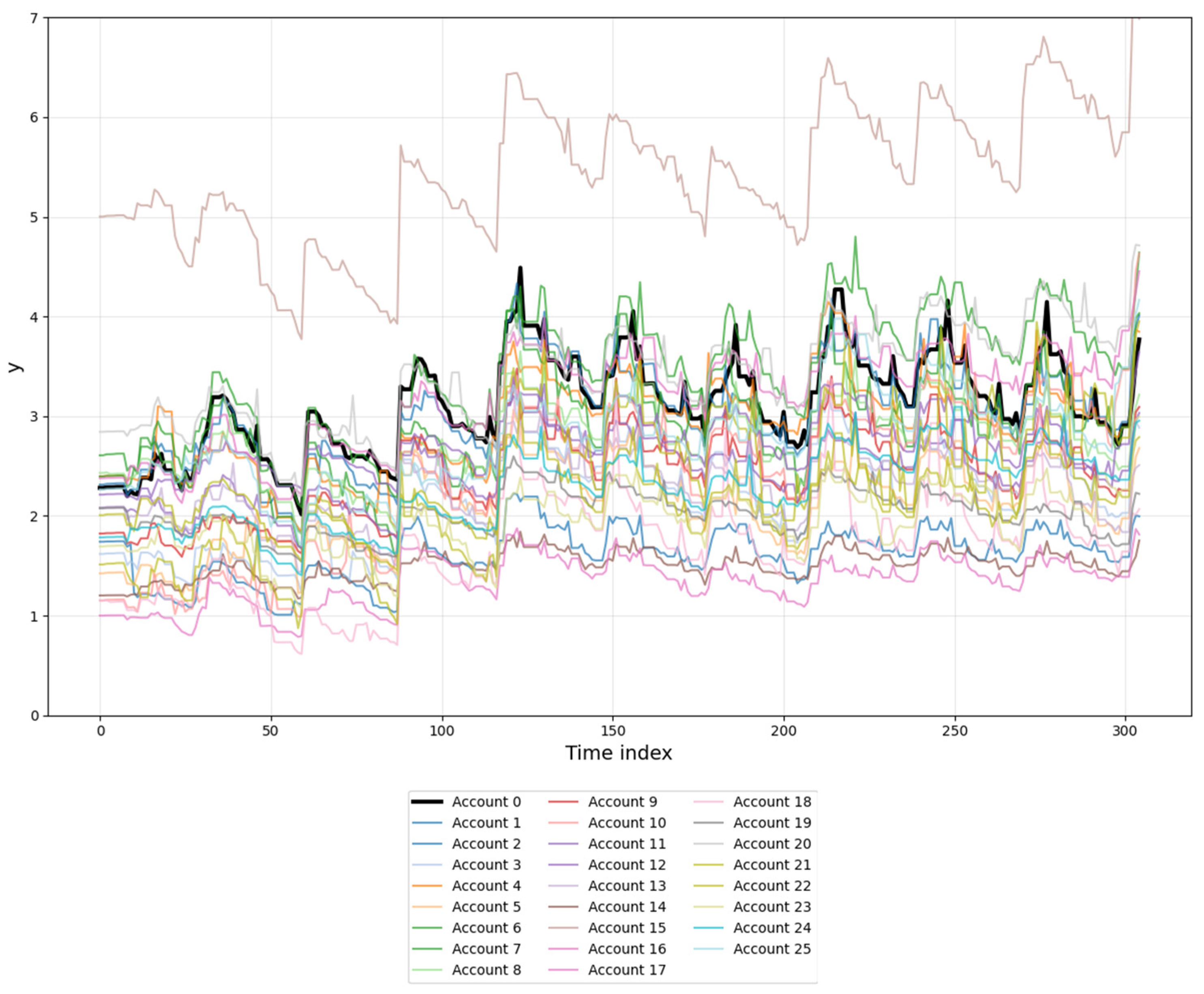
As a practical example, time series are taken representing anonymized data on daily account balances of bank customers over one year. The dataset consists of 26 accounts: one reference (Account 1) and 25 comparison series. Their dynamics are shown in Figure 1.

In contrast to the general theory of reconstruction in jet spaces of arbitrary dimension, for the analysis of financial time series it is natural to restrict ourselves to a two-dimensional phase portrait. A financial series $y\left(t\right)$ is interpreted as one coordinate of the trajectory of some dynamical system, and its derivative $\dot{y}\left(t\right)$ as the second coordinate. This approach is minimal, visual, and allows for the use of the classical apparatus of differential geometry of plane curves.

Let the time series $y\left(t\right)$ be the result of a dynamical system defined on a manifold $\mathrm{M}$ on which a Lie transformation group is defined. The infinitesimal generator of the group is a vector field that can be recovered via Lie series [52,53]. If we consider the operation with respect to time, the Lie series becomes a Taylor series. Being an invariant of the group, the series can thus characterise the transformation group. Using numerical differentiation, we consider the locus of points in the coordinate space. In turn, a corresponding transformation group can be introduced on this manifold.

Definition 1.

A model is called structurally stable with respect to $G$ if for any sufficiently small perturbation of its vector field there exists a transformation $g\in G$ such that the perturbed system is topologically equivalent to the original after a coordinate change from $G$.

In contrast to general reconstruction methods that operate in arbitrary-dimensional phase spaces (e.g., Takens’ delay embedding), for financial time series, we adopt a minimal two-dimensional representation. A time series $y\left(t\right)$ is interpreted as one coordinate of the trajectory of some underlying dynamical system, and its first derivative $\dot{y}\left(t\right)$ as the second coordinate. This choice is natural for financial data, where the shape of the series and its rate of change carry essential information about the system’s dynamics.

Formally, we consider the first jet space $J^1(\mathbb{R},\mathbb{R})$ with local coordinates $(t,y,\dot{y})$. For a given series $y\left(t\right)$, we construct the integral curve

$$r\left(t\right)=\left(y\right(t),\hspace{0.33em}\dot{y}(t){)}^{\mathrm{\top }}\in {\mathbb{R}}^2.$$

This curve is parametrised by time $t$, but its geometric shape (up to reparametrisation) is determined by the sequence of points in the $(y,\dot{y})$-plane.

The main idea of our approach is to find a transformation group $G$ acting on the coordinates $(y,\dot{y})$ such that all series in the cluster are related by elements of $G$. In our experiments, we consider the group

$$G=\mathrm{A}\mathrm{f}\mathrm{f}\left(J^1\right)\times SO\left(2\right),$$

where $\mathrm{A}\mathrm{f}\mathrm{f}\left(J^1\right)$ denotes affine transformations of the $(y,\dot{y})$ coordinates (translation and scaling), and $SO\left(2\right)$ is the group of rotations. The full group $G$ thus consists of transformations

$$\tilde{r}=S\hspace{0.17em}{R}_{\theta }\hspace{0.17em}r+b, S=\left(\begin{array}{cc}{s}_y& 0\\ 0& s_{\dot{y}}\end{array}\right), s_y>0,\hspace{0.25em}{s}_{\dot{y}}>0, R_{\theta }\in SO(2), b\in {\mathbb{R}}^2,$$

i.e., diagonal scaling (allowing different scales for $\mathrm{y}$ and $\dot{\mathrm{y}}$), rotation and translation. This group is a Lie group, and its Lie algebra generates the corresponding Lie series, which we use for search for transformations in the group.

To determine whether two curves are related by an element of $G$, we need a quantity that is invariant under the rotational part and behaves predictably under scaling. Classical differential geometry provides such a quantity: the Euclidean curvature $\kappa \left(s\right)$ as a function of the arc-length parameter $s$. It is well known that:

• Rotation of the curve leaves $\kappa \left(s\right)$ unchanged.
• Uniform scaling by a factor $\lambda$ multiplies $\kappa \left(s\right)$ by $1/\lambda$.
• Two curves with the same function $\kappa \left(s\right)$ are identical up to a rigid motion (translation and rotation).

Thus, $\kappa \left(s\right)$ is a complete invariant under the subgroup of rotations (up to translation). In practice, we work with discrete, noisy data and cannot compare $\kappa \left(s\right)$ point-wise. Instead, we compare the distributions of curvature values over the entire curve. Moreover, since the curves may differ by a general affine transformation of the $(y,\dot{y})$ coordinates (which is not a symmetry but may arise from different scales or offsets), we first normalise each curve (centre and scale) to remove these effects. After normalisation, the remaining transformation is a rotation, and the curvature distributions should coincide.

Importantly, $\kappa \left(s\right)$ depends on the derivatives of $r\left(t\right)$ up to third order ($\dot{y},\ddot{y},y^{\left(3\right)}$), hence it is an object in the third jet space $J^3$. A change in coordinates in $J^3$ (e.g., an affine transformation of the curvature values themselves) does not affect the shape of the distribution after standardisation. This justifies our procedure: we compute curvature, standardise its distribution, and compare the resulting distributions using a statistical test.

Since our method relies on Lie group transformations, we recall some basic notions. A Lie group $G$ is a smooth manifold that is also a group, with smooth multiplication and inversion. Its associated Lie algebra $\mathfrak{g}$ is the tangent space at the identity, equipped with the Lie bracket. The Lie algebra can be identified with the set of infinitesimal generators—vector fields on the manifold on which $G$ acts.

For a one-parameter subgroup $\mathrm{e}\mathrm{x}\mathrm{p}\left(tX\right)$ generated by $X\in \mathfrak{g}$, the corresponding finite transformation is obtained by exponentiating the vector field $X$:

$$\mathrm{e}\mathrm{x}\mathrm{p}(tX)r=r+tXr+{\displaystyle \frac{t^2}{2!}}{X}^{2}r+\cdots ,$$

where the action of $X$ on a point $r$ is given by the differential operator. This series is the Lie series. In practice, for matrix Lie groups, the exponential map is expressed via the matrix exponential, which converges everywhere.

In our setting, we consider the Lie algebra $\mathfrak{g}$ of the group $G=\mathrm{A}\mathrm{f}\mathrm{f}\left(J^1\right)\times SO\left(2\right)$. Its elements are vector fields on ${\mathbb{R}}^2$ that generate translations, uniform scaling, and rotations.

Theorem 1.

(Curvature as a necessary invariant for equivalence under $G$). Let $r\left(t\right)=\left(y\right(t),\dot{y}(t\left)\right)$ be a smooth curve in the $(y,\dot{y})$-plane, and let $\kappa \left(s\right)$ be its Euclidean curvature as a function of the arc-length parameter $s$. Then:

1. Invariance under rotations. If $r$ is rotated by $R_{\theta }\in SO\left(2\right)$, i.e., $\tilde{r}\left(t\right)=R_{\theta }r\left(t\right)$, then $\tilde{\kappa }\left(s\right)=\kappa \left(s\right)\hspace{0.25em}\forall s$.

2. Behaviour under the full group $G=Aff\left(J^1\right)\times SO\left(2\right)$. Up to an affine change in coordinates in $J^1$ (translation and diagonal scaling), the standardised curvature distribution is invariant.

3. Change in coordinates in $J^3$ and standardisation. The curvature $\kappa \left(s\right)$ is an object in $J^3$; comparing standardised curvature distributions is equivalent to checking equality of curvature functions up to an affine transformation in $J^3$.

Proof. 

$$

1. Rotations preserve the Euclidean metric, hence curvature (which depends only on the metric and its derivatives) is invariant.

2. For the full group $G=Aff\left(J^1\right)\times SO\left(2\right)$, we first apply an affine coordinate change in $J^1$: we centre each curve and scale each coordinate by its standard deviation. This operation is itself an element of $Aff\left(J^1\right)$ (translation and diagonal scaling). After this normalisation, all curves have unit variance in both coordinates, so any further transformation from $G$ that preserves the standardised curvature distribution must be a rotation (since translations and scalings have been removed). Rotations do not change curvature. The $z$-score standardisation of $\kappa$ removes the remaining isotropic scale factor, if any. Hence the standardised curvature distribution is invariant under the entire group $G$ up to the preliminary normalisation, which is part of the equivalence relation.

3. An affine transformation of curvature values $\tilde{\kappa }=a\kappa +b$ changes the mean and variance; standardisation makes the distributions invariant under such transformations. Thus, the standardised distribution ($z$-score) of $\kappa$ is invariant under any affine reparametrisation of the curvature values 3. □

Corollary 1.

From points 1–3 of Theorem 1—Necessary condition for equivalence under $G$. If two curves are related by a transformation from $G$ (i.e., a similarity plus translation), then their standardised curvature distributions coincide. This provides a practical necessary criterion for testing the hypothesis that the series belong to the same symmetry class. The converse is not generally true, but distributional equality is a strong indicator that can be tested statistically.

Corollary 2.

For discrete time series, numerical derivatives allow for the computation of $\kappa \left(s\right)$. If the standardised curvature distributions of two series are statistically indistinguishable (e.g., by a Kolmogorov–Smirnov test), this supports the hypothesis that the curves are related by a rotation (up to preliminary normalisation and an affine coordinate change in $J^3$). Thus, curvature provides a practical criterion for identifying structurally similar time series.

We now explicitly construct the Lie algebra $\mathfrak{g}$ of the group $G=\mathrm{A}\mathrm{f}\mathrm{f}\left(J^1\right)\times SO\left(2\right)$. Its Lie algebra $\mathfrak{g}$ is spanned by the following infinitesimal generators (vector fields on ${\mathbb{R}}^2$):

$$X_1={\partial }_y, X_2={\partial }_{\dot{y}}, X_3=y\hspace{0.17em}{\partial }_y, X_4=\dot{y}\hspace{0.17em}{\partial }_{\dot{y}}, X_5=-\hspace{0.17em}\dot{y}\hspace{0.17em}{\partial }_y+y\hspace{0.17em}{\partial }_{\dot{y}}.$$

Here $X_1,X_2$ generate translations, $X_3,X_4$ generate independent scalings along $\mathrm{y}$ and $\dot{\mathrm{y}}$, and ${\mathrm{X}}_5$ generates rotations. The corresponding finite transformation is obtained via the exponential map and has the form $r\mapsto S{R}_{\theta }r+b$ with $S=\mathrm{d}\mathrm{i}\mathrm{a}\mathrm{g}(e^{\alpha },e^{\beta })$, $R_{\theta }=e^{\theta X_5}$, and $\mathrm{b}$ from $X_1,X_2$.

These vector fields act on functions by differentiation; their action on a point $r$ is given by $X_{i}r$ evaluated at $r$. The non-zero Lie brackets are:

$$[X_1,X_3]=X_1, [X_2,X_4]=X_2, [X_1,X_5]=X_2, [X_2,X_5]=-X_1,$$

with all other brackets vanishing. In particular, $X_3$ and $X_4$ (the scaling generators) commute with each other and with ${\mathrm{X}}_5$ (the rotation generator), so the scaling and rotation parts form an abelian subalgebra.

Any element $\mathrm{X}\in \mathfrak{g}$ can be written as

$$X=\alpha X_1+\beta X_2+\gamma X_3+\delta X_4+\epsilon X_5,$$

with parameters $\alpha ,\beta ,\gamma ,\delta ,\epsilon \in \mathbb{R}$. The corresponding finite transformation is given by the exponential map. Since the scaling generators $X_3,X_4$ and the rotation generator $X_5$ commute pairwise, we have

$$\mathrm{e}\mathrm{x}\mathrm{p}(\gamma X_3+\delta X_4+\epsilon X_5)=S{R}_{\theta },$$

where

$$S=\left(\begin{array}{cc}{e}^{\gamma }& 0\\ 0& e^{\delta }\end{array}\right), {\mathrm{R}}_{\mathsf{\theta }}=\left(\begin{array}{cc}\mathrm{c}\mathrm{o}\mathrm{s}\epsilon & -\mathrm{s}\mathrm{i}\mathrm{n}\epsilon \\ \mathrm{s}\mathrm{i}\mathrm{n}\epsilon & \mathrm{c}\mathrm{o}\mathrm{s}\epsilon \end{array}\right).$$

The translation part generated by $\alpha X_1+\beta X_2$ is simply translation by $b=(\alpha ,\beta {)}^{\top }$. Because translations do not commute with scaling and rotation, the overall exponential map yields the composition

$$\mathrm{e}\mathrm{x}\mathrm{p}\left(X\right)=T_b\circ S\circ R_{\theta },$$

where the scaling and rotation are applied first, followed by the translation. Thus,

$$\mathrm{e}\mathrm{x}\mathrm{p}\left(X\right)\hspace{0.17em}r=S{R}_{\theta }\hspace{0.17em}r+b.$$

The parameters $(S,R_{\theta },b)$ uniquely determine an element of $G$ and can be recovered from $(\mathsf{\alpha },\mathsf{\beta },\mathsf{\gamma },\mathsf{\delta },\mathsf{\epsilon })$. The found parameters are precisely the coefficients of the Lie series expansion, as they determine the element $\mathrm{e}\mathrm{x}\mathrm{p}\left(X\right)\in G$.

Thus, for the applied problem of series assumed to have a common structure, the procedure for finding invariants that confirms this assumption is as follows:

1. Initial similarity assessment (affine correction in $\mathrm{y}$). We load the original data and evaluate their similarity with respect to amplitude and shifts in $y$. As a first approximation, we apply an affine transformation $y_{\mathrm{corr}}=a\hspace{0.17em}y+b$, where $a,b$ are fitted by least squares to minimise the MSE with the reference series. If the resulting $R^2$ values satisfy the researcher’s criteria, the procedure may stop; otherwise, we proceed to the next steps.

2. Derivative computation, filtering, curvature construction, and invariance test. We compute the derivatives using finite differences (invariant in the jet space):

$${\dot{y}}_i={\displaystyle \frac{y_{i+1}-y_{i-1}}{2h}}+O\left(h^2\right),$$

$${\ddot{y}}_i={\displaystyle \frac{y_{i+1}-2y_i+y_{i-1}}{h^2}}+O\left(h^2\right),$$

$$y_i^{\left(3\right)}={\displaystyle \frac{y_{i+2}-2y_{i+1}+2y_{i-1}-y_{i-2}}{2h^3}}+O(h^2),$$

with $h=1$ day.

3. In the first jet space $J^1$, we take low-pass filtered signals and compute the curvature at each point. Such filtering guarantees smoothness and extracts the main components that affect the shape of the curve in the jet space. According to Theorem 1, the curvatures $\kappa \left(s\right)$ are invariants in the jet space, but their exact coincidence is not guaranteed—only up to a coordinate change. We construct histograms of curvature distributions for each series, then scale and shift them (a permissible coordinate change). We compare the number of curvature values that match those of the reference series (within a tolerance). If the invariant is preserved, accounting for noise and filtering effects, the series pass the curvature-invariance test and can be used for further computations.

4. Construction of transformations using the Lie series for the group $G=Aff\left(J^1\right)\times SO\left(2\right)$. We seek a transformation that maps one series to another, taking into account the group $G=Aff\left(J^1\right)\times SO\left(2\right)$, where $Aff\left(J^1\right)$ acts on the $\left(y,\dot{y}\right)$ coordinates (translation and scaling) and $SO\left(2\right)$ acts as rotations. We minimise the distance between the original (unfiltered) series and the reference. For the search, we use a Lie series determined by the Lie algebra built on the group $G$. After computing the coefficients of the Lie series (since the optimisation is performed in the time domain, we can use a Taylor series with higher-order terms), the obtained coefficients allow us to compute the transformation group for each series, i.e., we obtain the shift, scaling, and rotation in the jet space $J^1$.

5. Application of the found transformations and final evaluation. We apply the found transformations to the jet space $J^1$ (without filtering or smoothing, using the first derivative from finite differences, which is invariant in the jet space). We then evaluate $R^2$. If the value meets the researcher’s goals, the series is considered symmetric to the reference.

6. Interval assessment for selected series. For the selected series (those that passed the invariance test and the final alignment), we apply the found transformations and evaluate the group and interval characteristics according to the required criteria, such as PICP (Prediction Interval Coverage Probability) and PINAW (Prediction Interval Normalised Average Width).

For curvature computation, we apply a low-pass filter to the original signal. This filtering guarantees smoothness and extracts the main shape-forming components, allowing us to estimate the curvature in the jet space J¹ without high-frequency noise distorting the result. In contrast, for the identification of the transformation (i.e., the search for the group parameters using the Lie series), we use the original, unfiltered data and compute the first derivative via finite differences. This choice is deliberate: finite differences are invariants in the discrete jet space, and any additional smoothing (such as Savitzky–Golay or Tikhonov regularisation) would alter the higher derivatives and break the invariance property that we aim to identify. The fact that the method produces consistent results across all 25 series, with correlation dimensions in the range 1.27–1.57, demonstrates its robustness on real financial data with the given daily sampling step.

4. Results

All experiments were performed on real financial data—26 daily time series of bank account balances (anonymised: Account 0 is the reference, Accounts 1–25 are test series). Each series contains 305 observations.

The results presented below correspond to the steps of the developed methodology and to the code provided in the Supplementary Materials. All computations, figures for all series, and comprehensive summary tables with criteria are available at the link. Everything can be viewed and downloaded, except for the original time series, which remain confidential.

1. Affine Correction along $Y$.

To assess the potential for aligning the series through amplitude and level adjustments, a simple affine transformation $y_{\mathrm{corr}}=a\cdot y+b$ was applied, with coefficients a and b estimated by least squares minimisation of the mean squared error with respect to the reference series. The goal was to evaluate how well the series could be matched using only amplitude scaling and vertical shift. 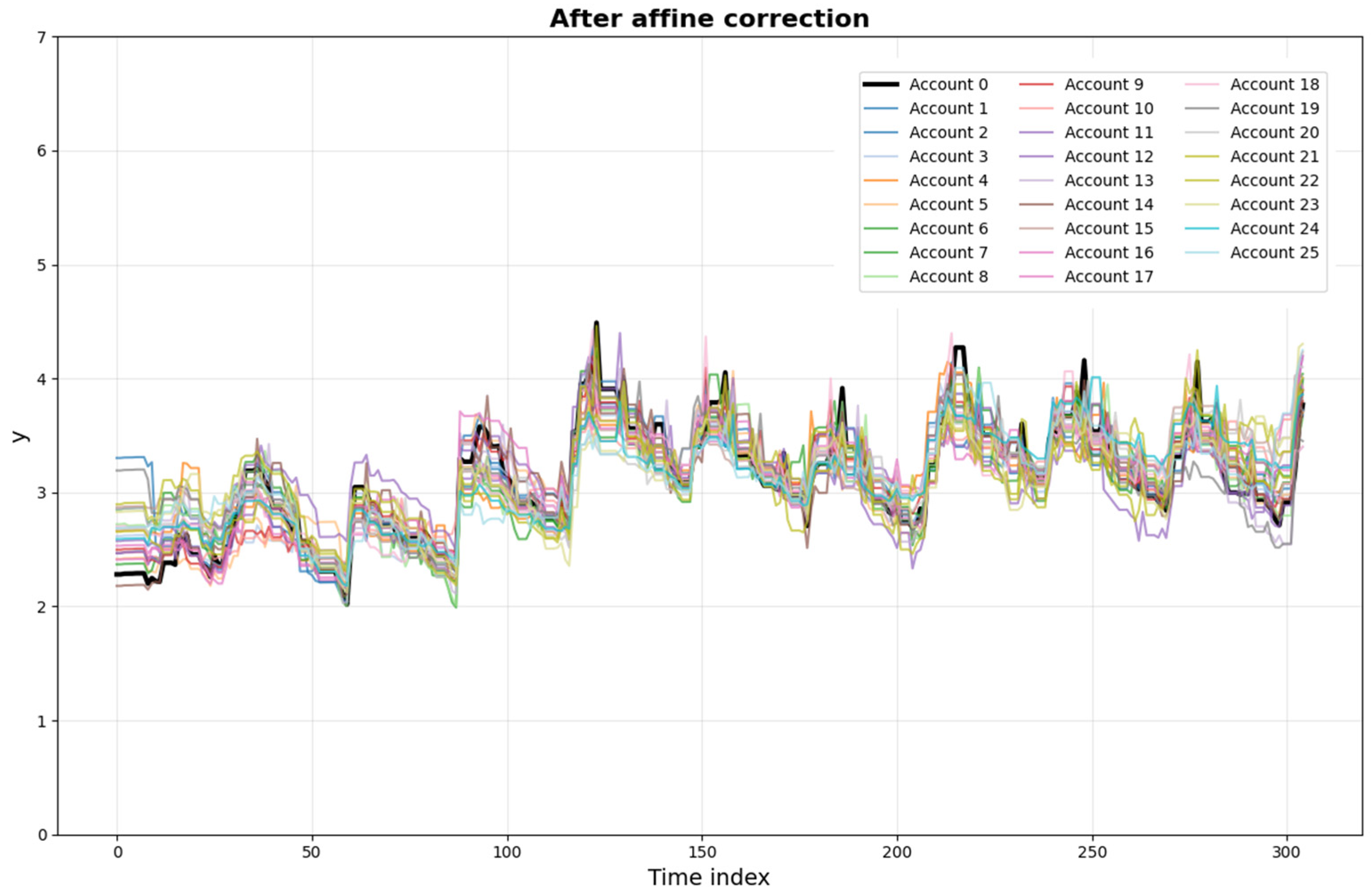The results yielded a mean coefficient of determination $R^2$ = 0.732, ranging from 0.58 to 0.88 across the 25 series. As shown in Figure 2, the spread of the series is substantially reduced after correction, with most series lying close to the reference trajectory.

Distribution of $R^2$ after affine correction:

• 12 series: $R^2>0.8$
• 8 series: $0.7\le R^2\le 0.8$
• 5 series: $0.6\le R^2<0.7$
• 1 series: $R^2<0.6$

If some series meet the researcher’s requirements for a given application, they can be selected for the cluster and used to determine the “true” financial transformations. The subsequent steps may be performed only for a subset of series; however, in this evaluation we apply further transformations to all series for completeness.

Table 1. Application of affine transformations to series.

Account	R2	MSE	RMSE	MAE	MAPE (%)	a	b
Account 1	0.6882	0.0742	0.2725	0.1816	6.1255	1.4849	0.7174
Account 2	0.8400	0.0381	0.1951	0.1504	4.8097	0.8961	0.396
Account 3	0.8071	0.0459	0.2143	0.1657	5.3818	0.8687	1.2118
Account 4	0.7013	0.0711	0.2667	0.2127	6.9877	0.8478	0.6314
Account 5	0.8104	0.0451	0.2125	0.1611	5.2338	1.0217	0.9619
Account 6	0.8157	0.0439	0.2095	0.1597	5.061	0.7173	0.6514
Account 7	0.7412	0.0616	0.2482	0.1966	6.5607	0.8338	0.6773
Account 8	0.7938	0.0491	0.2216	0.1641	5.5236	1.1761	−0.1388
Account 9	0.8356	0.0391	0.1979	0.15	4.7729	1.0256	0.6291
Account 10	0.6553	0.0821	0.2865	0.2195	7.0279	0.5059	1.8886
Account 11	0.6568	0.0817	0.2859	0.2374	7.7858	1.7469	−1.4008
Account 12	0.8396	0.0382	0.1954	0.1551	5.0534	1.0403	0.4076
Account 13	0.7741	0.0538	0.2319	0.1798	6.0818	1.2744	0.2005
Account 14	0.8808	0.0284	0.1685	0.135	4.3108	3.1164	−1.5665
Account 15	0.6411	0.0855	0.2923	0.2197	7.2696	0.5725	0.0082
Account 16	0.7716	0.0544	0.2332	0.1727	5.4808	1.706	0.8262
Account 17	0.7602	0.0571	0.2389	0.1832	5.8473	0.8594	0.3672
Account 18	0.734	0.0633	0.2517	0.1993	6.478	0.764	1.8237
Account 19	0.6485	0.0837	0.2893	0.207	7.0227	1.79	−0.5248
Account 20	0.6323	0.0875	0.2959	0.2287	7.3606	0.7627	0.506
Account 21	0.6716	0.0782	0.2796	0.225	7.2676	0.5529	1.8189
Account 22	0.6812	0.0759	0.2755	0.2226	7.661	1.2812	0.3238
Account 23	0.5782	0.1004	0.3169	0.2389	7.8803	1.1345	0.9066
Account 24	0.7196	0.0668	0.2584	0.2028	6.5085	1.0843	0.6567
Account 25	0.6196	0.0906	0.3009	0.2313	7.5734	0.8204	0.8298

reports the detailed metrics for the affine correction.

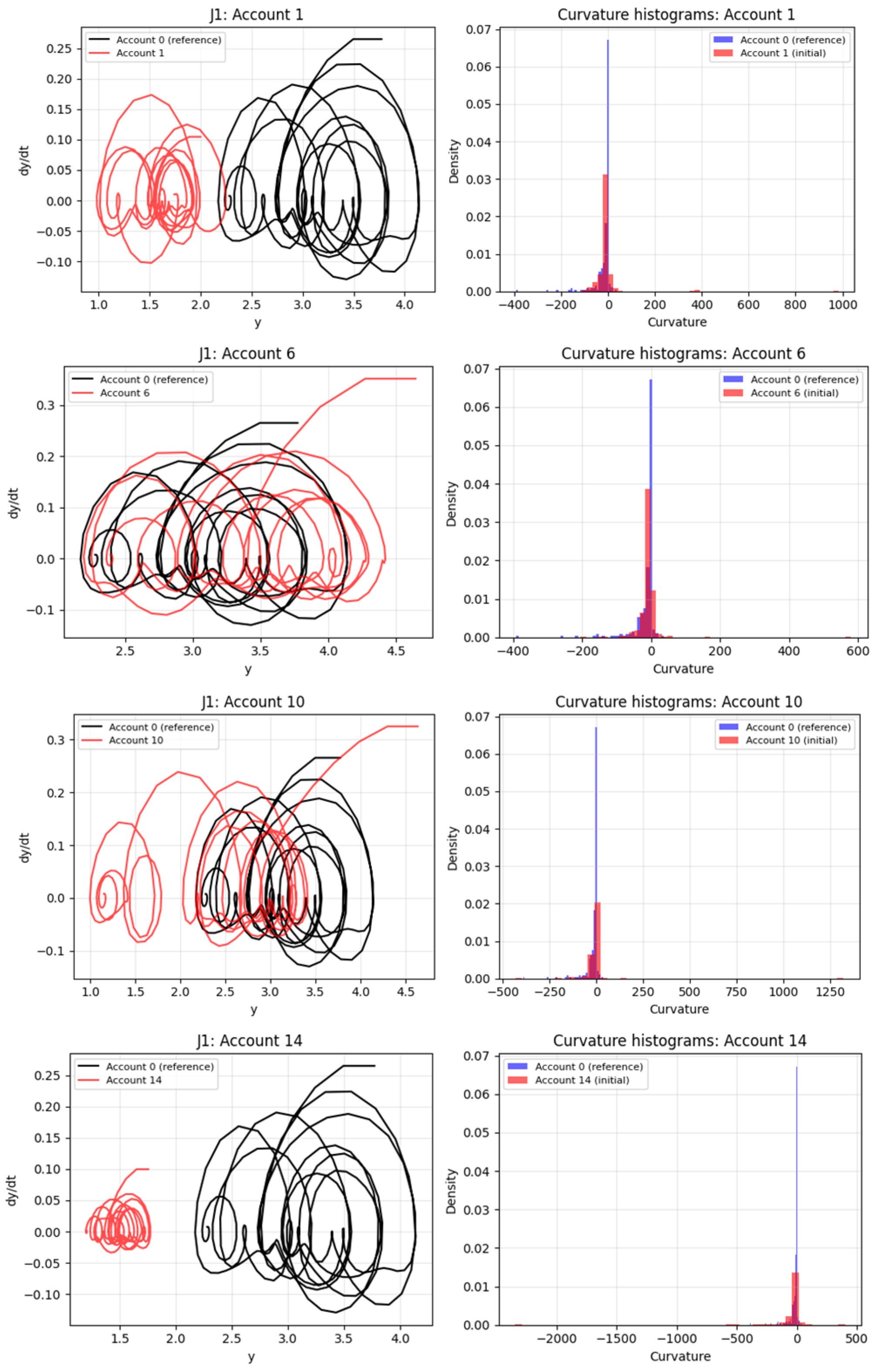
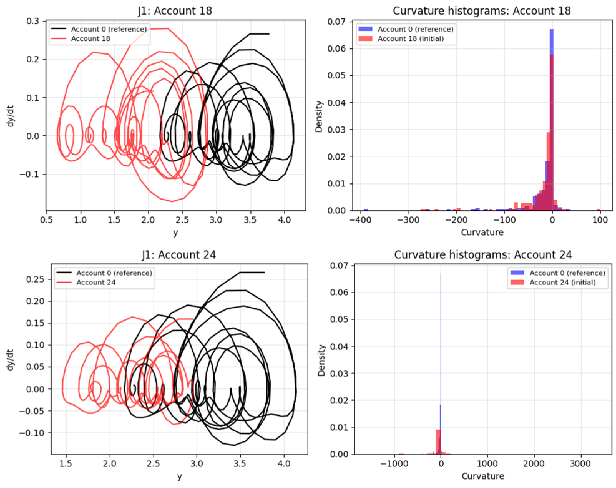
2. Curvature Test. The purpose of this step was to verify whether the distributions of curvature values for the transformed series coincide with that of the reference series. For each series, the curvature $\kappa \left(s\right)$ was computed as a function of the natural parameter s, and the empirical distributions were compared with the reference using the Kolmogorov–Smirnov test. After normalisation by mode and interquartile range, the test yielded p-values above 0.05 for all 25 series. The average fraction of matching curvature values within a 10% tolerance band was 88.7%, with the lowest value of 83.6% observed for Account 20. It is emphasised that the Kolmogorov–Smirnov test is used here as a screening tool, not as a formal equivalence test; failure to reject the null hypothesis does not prove that the distributions are identical, and no adjustment for multiple comparisons is performed. The fraction of matching curvature values within the tolerance band provides a complementary indication of similarity, but the results should be interpreted with caution. 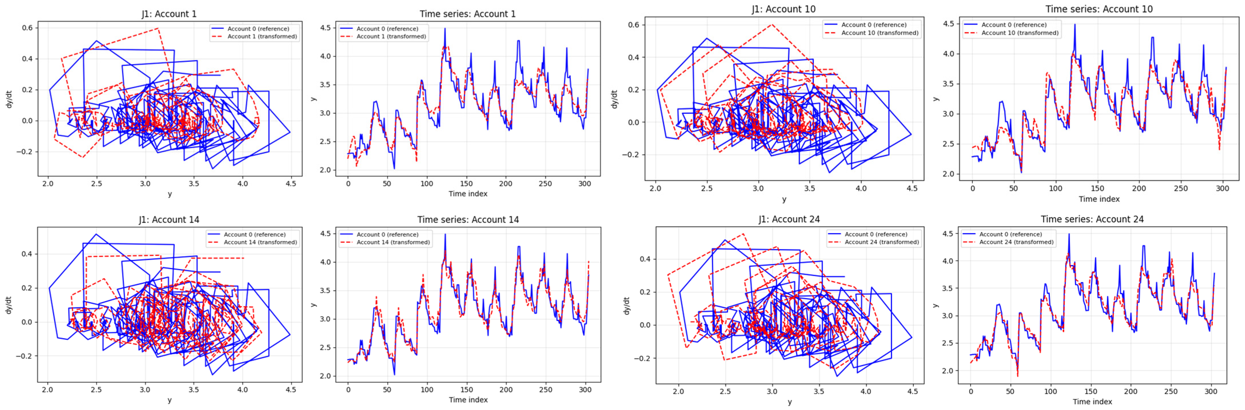Figure 3 shows some curvature plots and histograms (all figures and numbers are available via the link in the Supplementary File).

Match fractions for all series (10% tolerance of the reference range): 2 accounts—90% and more; 22 accounts = 85–90%;1 accounts (15) = 83.28%.

Thus, all series passed the curvature invariance test, confirming the existence of the desired group $G$.

3. Results of the Search for Transformations in $Aff\left(J^1\right)\times SO\left(2\right)$ Results According to the developed methodology, transformation coefficients were obtained (their values are given in

Table 2. Identification $\mathrm{A}\mathrm{f}\mathrm{f}\left(J^1\right)\times \mathrm{S}\mathrm{O}\left(2\right)$.

Account	R2	Corr	MSE	s_y	s_dy	shift_y	shift_dy	phi_deg
Account 1	0.8564	0.9254	0.0342	0.4970	0.6915	1.6799	0.0005	103.6565
Account 2	0.8978	0.9475	0.0243	0.5248	1.0423	1.0742	−0.0014	106.1235
Account 3	0.8673	0.9313	0.0316	0.5822	0.1075	1.6935	−0.0005	115.1757
Account 4	0.8344	0.9135	0.0394	0.9375	1.3974	0.8716	−0.0013	107.2220
Account 5	0.8507	0.9223	0.0355	0.1167	0.6740	2.1523	0.0007	−26.5584
Account 6	0.9207	0.9595	0.0189	0.5095	0.2015	0.7824	−0.0005	147.8324
Account 7	0.9128	0.9554	0.0208	0.8826	0.8907	0.6395	−0.0002	−129.8782
Account 8	0.9049	0.9513	0.0226	0.2303	0.2165	1.9858	−0.0005	94.8330
Account 9	0.8865	0.9415	0.0270	0.9807	0.9637	0.7311	0.0008	109.9378
Account 10	0.8580	0.9263	0.0338	1.1610	0.3572	1.0345	0.0003	48.2452
Account 11	0.8981	0.9477	0.0243	0.6225	1.9392	0.4487	0.0001	−148.6491
Account 12	0.9219	0.9367	0.0318	1.3475	1.7052	−0.2910	−0.0023	114.5646
Account 13	0.9152	0.9567	0.0202	0.2483	0.6411	1.4944	0.0007	105.8854
Account 14	0.9169	0.9575	0.0198	0.0306	2.0243	0.9656	−0.0007	55.4205
Account 15	0.8655	0.9303	0.0320	0.3051	0.9781	0.1909	−0.0008	72.8668
Account 16	0.8454	0.9195	0.0368	0.8064	0.3783	2.5212	−0.0006	−33.9530
Account 17	0.9051	0.9514	0.0226	0.2880	1.1250	0.6355	−0.0005	88.5598
Account 18	0.8757	0.9358	0.0296	0.7832	0.1415	1.9686	−0.0000	125.1550
Account 19	0.8808	0.9385	0.0284	2.1629	2.2313	−0.4666	−0.0001	110.7449
Account 20	0.8791	0.9376	0.0288	0.3143	2.4041	0.2923	−0.0014	58.2220
Account 21	0.8250	0.9083	0.0417	0.7783	0.0975	1.5336	0.0025	−113.7225
Account 22	0.9050	0.9513	0.0226	1.8895	0.7426	−0.1563	−0.0002	−149.5987
Account 23	0.7807	0.8836	0.0522	0.9229	1.3684	1.4618	−0.0011	85.4494
Account 24	0.9122	0.9551	0.0209	1.8982	0.6595	−0.7372	0.0003	14.8014
Account 25	0.8265	0.8542	0.0729	2.0437	0.0123	−1.2176	−0.0025	155.5024

). The algorithm based on Lie series can be seen in detail in the Python (Google Colab) code provided at the link. Figure 4 shows several series and their transformation in the jet space. Full results are available via the link in the attached file.

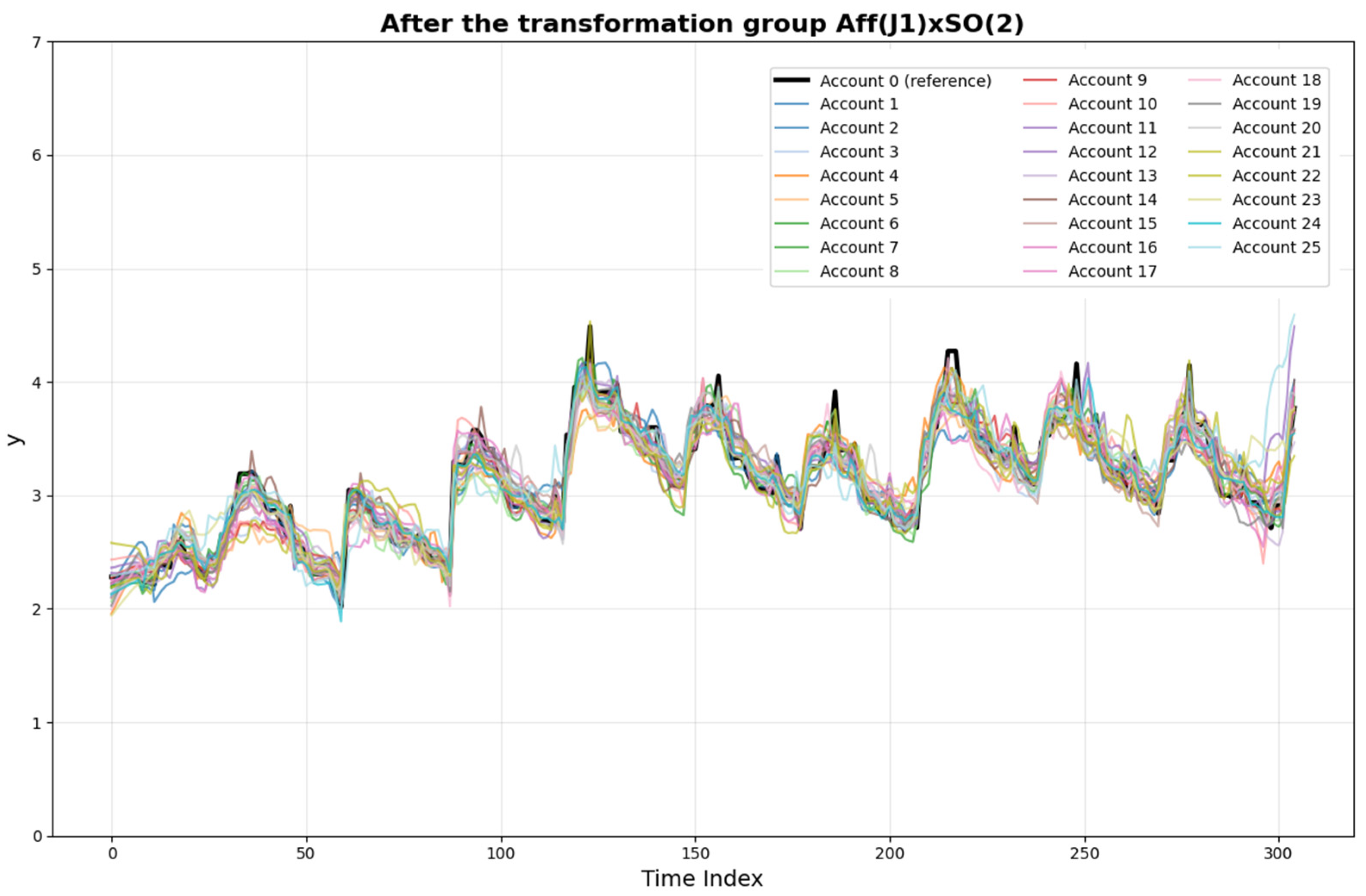
Results of the search for transformations in $Aff\left(J^1\right)\times SO\left(2\right)$ shown in Figure 5. The proposed method yielded a mean coefficient of determination $R^2$ = 0.876 after applying the transformations. This represents an average improvement of +0.144 over the affine correction baseline. For the 10 series that exhibited the poorest alignment after affine correction ($R^2$ < 0.7), the improvement ranged from +0.04 to +0.31, with the largest gains observed for the most problematic cases. The distribution of $R^2$ values after the transformation search shows that 24 series achieved $R^2$ > 0.8, and only one series fell within the range of 0.78.

A comparison was made using the Procrustes method [54] applied to the time series, which did not allow or the alignment of the series. This demonstrates that to obtain geometric invariants it is necessary to map a multidimensional model where the search for transformations is performed.

We also computed DTW distances. It is seen that our model outperforms all competitors in terms of $R^2$ for almost all series (except three series where DTW gives slightly better values). The obtained results allow us to solve the original problem—all considered series can be merged into a single cluster. For DTW alignment we used the DTAIDistance library. Negative values occur when the mean squared error after DTW exceeds the variance of the reference—this indicates that DTW fails to provide a meaningful alignment for those series under our evaluation protocol. To verify reproducibility, we also repeated the calculations with the dtw-python library; the results were analogous, ruling out artefacts of a particular implementation.

Table 3. Comparison $R^2$ across methods: affine, parametric, DTW-based, and Procrustes (The best results are indicated in bold).

Account	Affine	Group G	DTW	Procrust
Account 1	0.6882	0.8564	−5.4152	0.5561
Account 2	0.8400	0.8978	0.9486	0.6882
Account 3	0.8071	0.8673	0.4925	0.6950
Account 4	0.7013	0.8344	0.8995	0.5875
Account 5	0.8104	0.8507	0.0063	0.6504
Account 6	0.8157	0.9207	0.8346	0.6790
Account 7	0.7412	0.9128	0.8990	0.6224
Account 8	0.7938	0.9049	0.8502	0.6479
Account 9	0.8356	0.8865	0.6815	0.6507
Account 10	0.6553	0.8580	0.6406	0.5213
Account 11	0.6568	0.8981	0.6137	0.5168
Account 12	0.8396	0.9219	0.6754	0.7434
Account 13	0.7741	0.9152	0.1131	0.6138
Account 14	0.8808	0.9169	−8.2052	0.7367
Account 15	0.6411	0.8655	−7.6676	0.5408
Account 16	0.7716	0.8454	−6.6706	0.6512
Account 17	0.7602	0.9051	0.9038	0.6170
Account 18	0.7340	0.8757	0.1034	0.5699
Account 19	0.6485	0.8808	−1.1634	0.5366
Account 20	0.6323	0.8791	0.7926	0.5203
Account 21	0.6716	0.8250	0.6786	0.5649
Account 22	0.6812	0.9050	0.3376	0.6663
Account 23	0.5782	0.7807	0.1222	0.4679
Account 24	0.7196	0.9122	0.3534	0.5771
Account 25	0.6196	0.8265	0.8733	0.5697

compares $R^2$ across methods: affine, parametric, DTW-based, and Procrustes.

Experiment: Interval Forecasting: PICP and PINAW Analysis [55]. To evaluate the practical utility of the proposed alignment methods for interval forecasting, we conduct an experiment based on prediction intervals constructed around the reference series. The goal is to compare the coverage and width of intervals obtained after affine correction and after nonlinear parametric identification.

The reference series (Account 0) has a range of $2.474$ (in arbitrary units). We define a fixed prediction interval as:

$$\mathrm{Interval}=y_{\mathrm{ref}}\left(t\right)\pm \delta , \delta =0.10\times \mathrm{range}\left(y_{\mathrm{ref}}\right)=0.247.$$

Thus, the lower and upper bounds are $2.862$ and $3.357$, respectively (mean values). This interval represents a tolerance band of $\pm 10\%$ of the reference range.

For each transformed series (both affine and nonlinear), we compute the Prediction Interval Coverage Probability (PICP):

$$\mathrm{PICP}={\displaystyle \frac{1}{N}}{\displaystyle \sum _{i=1}^N}\mathbb{I}\{y_{\mathrm{pred}}(t_i)\in [y_{\mathrm{ref}}(t_i)-\delta ,\hspace{0.33em}{y}_{\mathrm{ref}}(t_i)+\delta ]\},$$

where $\mathbb{I}\{\cdot \}$ is the indicator function.

Table 4. PICP per series for affine and nonlinear transformations (PINAW = 0.2).

Account	PICP (Affine)	PICP (Nonlinear)
Account 1	0.8328	0.9115
Account 2	0.8492	0.9443
Account 3	0.7443	0.9148
Account 4	0.6754	0.9148
Account 5	0.8000	0.9246
Account 6	0.8066	0.9410
Account 7	0.7213	0.8984
Account 8	0.7410	0.8951
Account 9	0.8328	0.9246
Account 10	0.6492	0.9115
Account 11	0.5869	0.9049
Account 12	0.7705	0.8984
Account 13	0.7770	0.8721
Account 14	0.8557	0.8754
Account 15	0.6492	0.8525
Account 16	0.7508	0.8557
Account 17	0.7016	0.8525
Account 18	0.6656	0.8590
Account 19	0.6984	0.8623
Account 20	0.6033	0.8262
Account 21	0.6098	0.8590
Account 22	0.6525	0.8066
Account 23	0.6328	0.7475
Account 24	0.6557	0.7902
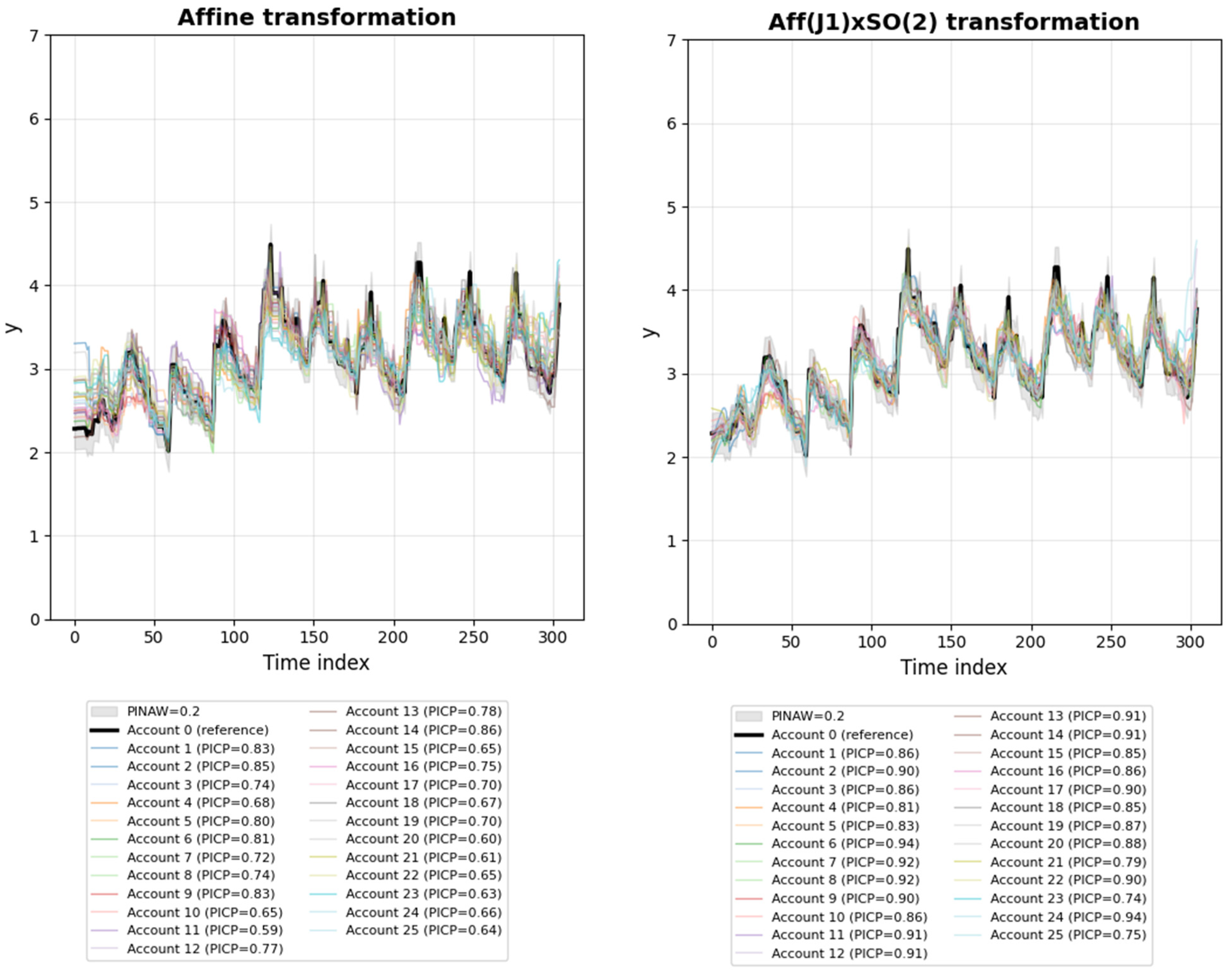
Account 25	0.6361	0.7443

reports the PICP values (PINAW = 0.2) for each of the 25 series for both methods.

Figure 6 shows the reference series, the fixed PINAW = 0.2, and all transformed series (affine on the left, $Aff\left(J^1\right)\times SO\left(2\right)$ on the right). The nonlinear transformation visibly clusters the series more tightly around the reference, especially in regions where the affine correction leaves larger deviations.

The interval forecasting experiment confirms that the transformation search not only improves the ${\mathrm{R}}^2$ and alignment quality but also provides more reliable and narrower prediction intervals. This makes the method suitable for practical applications where both coverage and interval width are critical, such as risk management and resource allocation.

5. Conclusions

A geometric method for identifying and aligning structurally similar time series has been developed, based on jet space reconstruction and Lie group theory. The main theoretical contribution is the proof that the Euclidean curvature of the integral curve in the first jet space ${\mathrm{J}}^1$ is a necessary invariant under the group $G=Aff\left(J^1\right)\times SO\left(2\right)$, which consists of translations, uniform scaling, and rotations in the $(y,\dot{y})$-plane. Unlike Takens’ delay embedding, which only guarantees topological equivalence, the proposed approach preserves metric and rotational symmetries, providing a coordinate-invariant criterion for clustering.

The practical procedure consists of three key steps: (i) the computation of derivatives and curvature from discrete series, (ii) the verification of curvature distribution invariance using the Kolmogorov–Smirnov test, and (iii) the recovery of transformation parameters (scale, rotation angle, translation) via the Lie series of the Lie algebra. The Python implementation is computationally efficient, as it operates on the entire series without fragmentation.

Experimental validation was performed on 26 daily bank account balance series (25 test series and one reference). The results confirm the effectiveness of the method. After the search for transformations in $G=\mathrm{A}\mathrm{f}\mathrm{f}\left(J^1\right)\times \mathrm{S}\mathrm{O}\left(2\right)$, the mean coefficient of determination $R^2$ increased from 0.732 (simple affine correction in $\mathrm{y}$) to 0.876, with all test series passing the curvature invariance test ($p>0.05$). The average fraction of matching curvature distributions within a 10% tolerance was 88.7%. In interval forecasting, the nonlinear alignment achieved a mean Prediction Interval Coverage Probability (PICP) of 0.8715 (compared to 0.7159 for affine correction) and a 30% reduction in the Prediction Interval Normalised Average Width (PINAW) while maintaining 100% coverage for the 95% prediction band. These results demonstrate that the geometric invariant not only enables accurate clustering but also provides a foundation for constructing narrow and robust prediction intervals.

Comparison with Procrustes analysis and DTW further highlights the advantage of working in the jet space: the proposed method consistently outperforms these baselines in terms of $R^2$, confirming that the curvature invariant captures essential structural information that is lost in amplitude-only or time-warping approaches.

It should be noted that the Kolmogorov–Smirnov test employed in the curvature invariance step serves as a necessary filter: series whose curvature distributions differ significantly from the reference are excluded from further alignment. The poor performance of DTW on the same data (Table 3) provides indirect evidence that the method does not produce spurious matches for arbitrary non-similar series. A systematic assessment of false positives on surrogate data remains beyond the scope of this work and is deferred to future research.

The developed geometric framework thus constitutes a powerful and practically applicable tool for analysing large collections of time series that share a common qualitative structure. The method can be applied in various domains, including finance, economics, and sensor data processing, where clustering, alignment, and interval forecasting are critical. Future work will explore extensions to higher-dimensional jet spaces and adaptive filtering to handle noisier data.