Fourier and Shape-Parameter Analysis of Compact Multiquadric RBF–HFD Approximations on Nonuniform Stencils

Abstract

This paper develops a compact analytical framework for multiquadric radial basis function–Hermite finite difference (MQ RBF–HFD) approximations on nonuniform meshes. The main contributions are a unified local operator formulation, uniform-grid reductions connected with compact finite difference schemes, and a Fourier and modified-wavenumber analysis for assessing spectral resolution. A local frozen-coefficient Fourier analysis is further introduced to study the effects of mesh nonuniformity and the MQ shape parameter. The shape-parameter dependence is examined through truncation-error constants, conditioning indicators, and Fourier-resolution measures. The MQ RBF–HFD formulas are also compared with PHS-polynomial RBF–FD and RBF–HFD variants, clarifying the relation between explicit shape-dependent compact weights and shape-parameter-free polynomially augmented constructions. Numerical experiments confirm the predicted convergence behavior and demonstrate the accuracy of the proposed compact analysis on small nonuniform stencils.

1. Introduction and Literature Review

The construction of accurate differentiation formulas on nonuniform meshes is one of the classical topics in numerical analysis [1]. Although polynomial finite difference (FD) formulas are simple and efficient on uniform grids, their order of accuracy may decrease substantially when the underlying mesh is irregular [2,3]. For a sufficiently smooth function g, a standard local differentiation formula at a node $x_i$ may be written as [4]:

$$g^{\left(p\right)}\left(x_i\right)\simeq \sum _{j\in {\mathcal{S}}_i}{w}_{ij}^{\left(p\right)}g\left(x_j\right),$$

(1)

where ${\mathcal{S}}_i$ is a local stencil and $w_{ij}^{\left(p\right)}$ are the corresponding FD weights. On nonuniform grids, the weights in (1) depend on the local spacings, and a small stencil may not provide the desired order of accuracy. Increasing the stencil width is one possible remedy, but it enlarges the local support of the approximation and may reduce the compact character of the resulting discretization; see, for example, the classical discussions in [5].

Radial basis function generated FD (RBF–FD) methods provide a flexible alternative to polynomial FD formulas. In RBF–FD methods, the weights in (1) are obtained by imposing exactness on RBFs rather than only on algebraic polynomials [6]. If $\varphi \left(r\right)$ is a radial kernel and $r=|x-x_j|$, a local RBF interpolant may be written as [7]:

$$s_i\left(x\right)=\sum _{j\in {\mathcal{S}}_i}{\lambda }_j\varphi \left(\right|x-x_j\left|\right).$$

In polynomially augmented RBF–FD methods [8], one instead uses

$$s_i\left(x\right)=\sum _{j\in {\mathcal{S}}_i}{\lambda }_j\varphi (|x-x_j|)+{\displaystyle \sum _{\ell =0}^d}{\chi }_{\ell }{p}_{\ell }\left(x\right),$$

where ${\{p_{\ell }\}}_{\ell =0}^d$ is a basis for a polynomial space. The local weights are then computed so that the action of the desired differential operator on $s_i$ is reproduced at $x_i$. Since the early development of RBF-FD formulas on irregular node layouts [9], this methodology has become an effective local meshfree approach for approximating differential operators on structured, unstructured, and scattered node sets [10].

A further improvement is obtained by combining RBF-FD ideas with compact or Hermite FD methodology [11]. In compact FD methods, derivative values at neighboring nodes are included in the approximation. Thus, instead of using only function values as in (1), one considers a relation of the form [5]:

$$g^{(p)}(x_i)\simeq \sum _{j\in {\mathcal{S}}_i}{a}_{ij}^{(p)}g(x_j)+\sum _{j\in {\mathcal{H}}_i}{b}_{ij}^{(p)}{g}^{(p)}(x_j),$$

(2)

where

$${\mathcal{H}}_i\subseteq {\mathcal{S}}_i\backslash \{x_i\}$$

denotes the neighboring nodes at which Hermite derivative information is used. The compact structure (2) is important because it can increase the accuracy and spectral resolution of the approximation without increasing the number of function-value nodes. Classical compact FD formulas are well known for their favorable modified-wavenumber behavior [4]. The RBF counterpart of this idea was developed in the compact RBF–FD framework of Wright and Fornberg [12], where compact FD-type formulas are generated from RBFs on scattered nodes. Further developments and applications of compact RBF-FD and Hermite-type schemes can be found in [13,14].

The present paper is based on the multiquadric (MQ) RBF–Hermite FD (RBF-HFD) weights derived in [15]. In that work, the MQ kernel [16]:

$$\varphi (r)=\sqrt{c^2+r^2},c>0,$$

(3)

was used on the three-node nonuniform stencil

$$\{x_{i-1},x_i,x_{i+1}\}=\{x_i-h,x_i,x_i+{\omega }_{i+1}h\},h>0,$$

(4)

to construct compact RBF–HFD formulas for the first and second derivatives. The first-derivative approximation was written in the form

$$\begin{array}{cc}\hfill g^{\prime }(x_i)& \simeq {\alpha }_{i-1}g(x_{i-1})+{\alpha }_{i}g(x_i)+{\alpha }_{i+1}g(x_{i+1})\hfill \\ \hfill & +{\beta }_{i-1}{g}^{\prime }(x_{i-1})+{\beta }_{i+1}{g}^{\prime }(x_{i+1}).\hfill \end{array}$$

(5)

while the second-derivative approximation was written as

$$\begin{array}{cc}\hfill g^{″}(x_i)& \simeq {\lambda }_{i-1}g(x_{i-1})+{\lambda }_{i}g(x_i)+{\lambda }_{i+1}g(x_{i+1})\hfill \\ \hfill & +{\mu }_{i-1}{g}^{″}(x_{i-1})+{\mu }_{i+1}{g}^{″}(x_{i+1}).\hfill \end{array}$$

(6)

Their local truncation errors have the form

$$\widehat{g^{\prime }}(x_i)-g^{\prime }(x_i)=C_1(c,{\omega }_{i+1};g)h^4+\mathcal{O}(h^5),$$

and

$$\widehat{g^{″}}(x_i)-g^{″}(x_i)=C_2(c,{\omega }_{i+1};g)h^3+\mathcal{O}(h^4).$$

Hence, the first-derivative formula is fourth-order accurate, whereas the second-derivative formula is third-order accurate on the compact three-node nonuniform stencil (4).

The purpose of the present paper is to develop a deeper analytical framework around the compact Formulas (5) and (6). The analysis focuses on their unified local operator structure, their uniform-grid specialization, their Fourier and modified-wavenumber behavior [17], their nonuniform frozen-coefficient Fourier symbols, their dependence on the MQ shape parameter, and their comparison with modern PHS-polynomial RBF–FD and RBF–HFD variants.

The Fourier analysis [18] starts from the uniform-grid specialization of (5) and (6). For a Fourier mode

$$g_j=exp(\mathrm{i}j\xi ),\xi =kh,$$

(7)

where k is the exact wave number and $\xi$ is the nondimensional wave number, the exact derivatives satisfy

$$g_j^{\prime }=\mathrm{i}k{g}_j,g_j^{″}=-k^2{g}_j.$$

A numerical differentiation formula defines a modified wave number $k_p^{*}$ through

$${\mathcal{D}}_p{g}_j={(\mathrm{i}{k}_p^{*})}^p{g}_j.$$

The deviation of $k_p^{*}$ from k measures the spectral resolution of the approximation. For the first derivative, we use

$${\mathcal{E}}_1(\xi )=\left|{\displaystyle \frac{k_1^{*}}{k}}-1\right|,$$

whereas for the second derivative we use

$${\mathcal{E}}_2(\xi )=\left|{\displaystyle \frac{{\left(k_2^{*}\right)}^2}{k^2}}-1\right|.$$

These quantities make it possible to compare MQ RBF–HFD formulas with classical FD, compact FD, and RBF–FD approximations on the basis of spectral resolution rather than Taylor error alone [19,20].

For nonuniform grids, the coefficients in (5) and (6) vary with the node $x_i$. Therefore, a single global Fourier symbol is no longer available. To handle this case, we use a local frozen-coefficient Fourier analysis. The local mesh ratio and shape ratio are fixed as

$$\omega ={\omega }_{i+1},\theta ={\displaystyle \frac{c}{h}}.$$

For the first derivative, the local frozen symbol has the form

$${\mathcal{D}}_1(\xi ;\omega ,\theta )={\displaystyle \frac{{\alpha }_{-}(\omega ,\theta )e^{-\mathrm{i}\xi }+{\alpha }_0(\omega ,\theta )+{\alpha }_{+}(\omega ,\theta )e^{\mathrm{i}\omega \xi }}{1-{\beta }_{-}(\omega ,\theta )e^{-\mathrm{i}\xi }-{\beta }_{+}(\omega ,\theta )e^{\mathrm{i}\omega \xi }}}.$$

(8)

The local modified wave number is then defined by

$$\mathrm{i}{k}_1^{*}(\xi ;\omega ,\theta )={\mathcal{D}}_1(\xi ;\omega ,\theta ).$$

The imaginary part of (8) describes the local dispersive behavior, while the real part describes local dissipation or growth. This local Fourier viewpoint is particularly useful because it shows how the mesh asymmetry $\omega$ and the shape ratio $\theta$ affect the compact approximation.

The MQ shape parameter c plays an important role in both accuracy and conditioning. If $M_i^{(p)}(c)$ denotes the local Hermite RBF matrix associated with the p-th derivative formula at the node $x_i$, its condition number is denoted by

$${\kappa }_i^{(p)}(c)=cond\left(M_i^{(p)}(c)\right).$$

(9)

A useful value of c should balance truncation error, conditioning, and Fourier resolution. This motivates a local selection principle of the form

$${\theta }_p^{*}=\underset{\theta \in [{\theta }_{min},{\theta }_{max}]}{arg\; min}\left\{{\gamma }_1{\mathcal{T}}_p(\omega ,\theta )+{\gamma }_{2}log\left(1+{\kappa }_i^{(p)}(\omega ,\theta )\right)+{\gamma }_3{\mathcal{R}}_p(\omega ,\theta )\right\},p=1,2,$$

(10)

where ${\mathcal{T}}_p$ is a truncation-error indicator, ${\kappa }_i^{\left(p\right)}$ is the local condition number, ${\mathcal{R}}_p$ is a Fourier-resolution indicator, and ${\gamma }_1,{\gamma }_2,{\gamma }_3\ge 0$ are balancing parameters. The criterion (10) is used in this paper as a diagnostic tool for understanding how the shape parameter affects the accuracy and stability of the local compact formulas.

The present paper also compares the MQ RBF–HFD framework with modern PHS-polynomial RBF–FD and RBF–HFD variants. In such methods, one frequently uses the shape-parameter-free polyharmonic spline kernel

$${\varphi }_{\mathrm{PHS}}\left(r\right)=r^{2m+1},m=0,1,2,\dots ,$$

(11)

together with a polynomial augmentation of the form

$$s_i\left(x\right)=\sum _{j\in {\mathcal{S}}_i}{\lambda }_j{\varphi }_{\mathrm{PHS}}(|x-x_j|)+{\displaystyle \sum _{\ell =0}^d}{\chi }_{\ell }{x}^{\ell }.$$

(12)

The use of PHS kernels with polynomial augmentation has become important in the modern RBF–FD literature because it can avoid direct shape-parameter selection while retaining high-order accuracy [21]. In the present work, the PHS-polynomial variants are not proposed as replacements for the explicit MQ RBF–HFD weights. Rather, they are used as contemporary benchmarks for comparing accuracy, conditioning, and Fourier-resolution behavior.

The main contributions of the paper can be summarized as follows. First, the uniform-grid reductions of these formulas are connected with compact FD approximations. Second, Fourier and modified-wavenumber analysis is used to study the spectral resolution of the uniform formulas. Third, a local frozen-coefficient Fourier analysis is introduced for the genuinely nonuniform case through (8). Fourth, the effect of the MQ shape parameter is examined through the condition number (9) and the selection principle (10). Fifth, the MQ RBF–HFD formulas are compared with PHS-polynomial RBF–FD and RBF–HFD variants based on (11) and (12).

The rest of the paper is organized as follows. Section 2 reviews the three-node MQ RBF–HFD weights. Section 3 introduces a unified compact RBF–HFD operator formulation. Section 4 derives the uniform-grid specialization of the weights. Section 5 presents the Fourier and modified-wavenumber analysis and then extends it to nonuniform stencils through local frozen-coefficient symbols, together with conditioning and shape-parameter indicators. Section 6 compares the MQ RBF–HFD formulas with PHS-polynomial RBF–FD and RBF–HFD variants. Numerical experiments are reported in Section 7. Finally, Section 8 gives the conclusions and discusses possible directions for future work. See Appendix A for clarifications on our notations.

2. Review of the Three-Node MQ RBF–HFD Weights

Let g be a sufficiently differentiable function on an interval $\mathsf{\Omega }\subset \mathbb{R}$. The MQ RBF used in [15] is (3). For notational compactness in this section, we use

$$\omega ={\omega }_{i+1}.$$

All formulas below are therefore written in terms of $\omega$, while the corresponding mesh ratio in the original stencil is the same quantity ${\omega }_{i+1}$.

Consider (5), if ${\mathcal{D}}_{1,i}^{\mathrm{MQHFD}}g$ denotes the right-hand side of (5), then

$${\mathcal{D}}_{1,i}^{\mathrm{MQHFD}}g={\alpha }_{i-1}g(x_{i-1})+{\alpha }_{i}g(x_i)+{\alpha }_{i+1}g(x_{i+1})+{\beta }_{i-1}{g}^{\prime }(x_{i-1})+{\beta }_{i+1}{g}^{\prime }(x_{i+1}).$$

The closed-form coefficients are

$$\begin{array}{cc}\hfill {\alpha }_{i-1}& ={\displaystyle \frac{{\omega }^2\left[\omega \left(-14c^2+31h^2\omega +62h^2\right)-28c^2-121h^2\right]}{7c^{2}h{(\omega +1)}^3}},\hfill \end{array}$$

(13)

$$\begin{array}{cc}\hfill {\alpha }_i& ={\displaystyle \frac{(\omega -1)\left(\frac{14}{\omega }-\frac{31h^2}{c^2}\right)}{7h}},\hfill \end{array}$$

(14)

$$\begin{array}{cc}\hfill {\alpha }_{i+1}& ={\displaystyle \frac{\frac{h^2\left(\omega (121\omega -62)-31\right)}{c^2}+14\left(\frac{1}{\omega }+2\right)}{7h{(\omega +1)}^3}},\hfill \end{array}$$

(15)

$$\begin{array}{cc}\hfill {\beta }_{i-1}& =-{\displaystyle \frac{{\omega }^2\left(7c^2-31h^2\omega +45h^2\right)}{7c^2{(\omega +1)}^2}},\hfill \end{array}$$

(16)

$$\begin{array}{cc}\hfill {\beta }_{i+1}& ={\displaystyle \frac{h^2(31-45\omega )\omega -7c^2}{7c^2{(\omega +1)}^2}}.\hfill \end{array}$$

(17)

The dimensional structure of these weights is

$${\alpha }_{i-1},{\alpha }_i,{\alpha }_{i+1}=\mathcal{O}\left(h^{-1}\right),{\beta }_{i-1},{\beta }_{i+1}=\mathcal{O}\left(1\right).$$

(18)

Thus, the first part of (5) has the usual derivative scaling, while the Hermite part is dimensionless and couples the unknown derivative values at the neighboring nodes.

The local truncation error associated with (5) is

$${\mathcal{D}}_{1,i}^{\mathrm{MQHFD}}g-g^{\prime }\left(x_i\right)=-{\displaystyle \frac{{\omega }^2\left(c^2{g}^{\left(5\right)}\left(x_i\right)+40g^{\left(3\right)}\left(x_i\right)\right)}{120c^2}}{h}^4+\mathcal{O}\left(h^5\right).$$

(19)

Therefore, the approximation (5) is fourth-order accurate on the three-node nonuniform stencil (4). In particular, if the local mesh ratio $\omega$ remains bounded away from zero and infinity, the leading order of the first-derivative error is governed by the factor

$$C_1(c,\omega ;g)=-{\displaystyle \frac{{\omega }^2\left(c^2{g}^{\left(5\right)}\left(x_i\right)+40g^{\left(3\right)}\left(x_i\right)\right)}{120c^2}}.$$

(20)

The error representation (19) will be used later when the shape-parameter dependence of the method is studied.

The second-derivative RBF–HFD approximation has the analogous procedure. Defining the local second-derivative operator by the right-hand side of (6), we write

$${\mathcal{D}}_{2,i}^{\mathrm{MQHFD}}g={\lambda }_{i-1}g\left(x_{i-1}\right)+{\lambda }_{i}g\left(x_i\right)+{\lambda }_{i+1}g\left(x_{i+1}\right)+{\mu }_{i-1}{g}^{″}\left(x_{i-1}\right)+{\mu }_{i+1}{g}^{″}\left(x_{i+1}\right).$$

The function-value weights for the second derivative are

$$\begin{array}{cc}\hfill {\lambda }_{i-1}& ={\displaystyle \frac{\omega {\mathcal{P}}_{\lambda ,-}(\omega ,c,h)}{98c^4{h}^2(\omega +1){({\omega }^2+3\omega +1)}^3}},\hfill \end{array}$$

(21)

$$\begin{array}{cc}\hfill {\lambda }_i& =-{\displaystyle \frac{3{\mathcal{P}}_{\lambda ,0}(\omega ,c,h)}{49c^4{h}^2{({\omega }^2+3\omega +1)}^3}},\hfill \end{array}$$

(22)

$$\begin{array}{cc}\hfill {\lambda }_{i+1}& ={\displaystyle \frac{{\mathcal{P}}_{\lambda ,+}(\omega ,c,h)}{98c^4{h}^2(\omega +1){({\omega }^2+3\omega +1)}^3}}.\hfill \end{array}$$

(23)

Here the polynomials in (21)–(23) are

$$\begin{array}{cc}\hfill {\mathcal{P}}_{\lambda ,-}(\omega ,c,h)& =14(84c^4+285c^2{h}^2-731h^4)\hfill \\ \hfill & +3(2352c^4+4914c^2{h}^2-14617h^4)\omega \hfill \\ \hfill & +(12936c^4+3444c^2{h}^2-10685h^4){\omega }^2\hfill \\ \hfill & +(7056c^4-21042c^2{h}^2+31075h^4){\omega }^3\hfill \\ \hfill & +(1176c^4+3444c^2{h}^2-37831h^4){\omega }^4\hfill \\ \hfill & +(14742c^2{h}^2+46265h^4){\omega }^5\hfill \\ \hfill & +15(266c^2{h}^2+137h^4){\omega }^6\hfill \\ \hfill & -39686h^4{\omega }^7-9744h^4{\omega }^8,\hfill \end{array}$$

(24)

$$\begin{array}{cc}\hfill {\mathcal{P}}_{\lambda ,0}(\omega ,c,h)& =7(28c^4+95c^2{h}^2-232h^4)\hfill \\ \hfill & +3(392c^4+819c^2{h}^2-2232h^4)\omega \hfill \\ \hfill & +(2156c^4+574c^2{h}^2-270h^4){\omega }^2\hfill \\ \hfill & +(1176c^4-3507c^2{h}^2+6200h^4){\omega }^3\hfill \\ \hfill & +2(98c^4+287c^2{h}^2-3663h^4){\omega }^4\hfill \\ \hfill & +(2457c^2{h}^2+6200h^4){\omega }^5\hfill \\ \hfill & +5(133c^2{h}^2-54h^4){\omega }^6\hfill \\ \hfill & -6696h^4{\omega }^7-1624h^4{\omega }^8,\hfill \end{array}$$

(25)

$$\begin{array}{cc}\hfill {\mathcal{P}}_{\lambda ,+}(\omega ,c,h)& =42(28c^4+95c^2{h}^2-232h^4)\hfill \\ \hfill & +2(3528c^4+7371c^2{h}^2-19843h^4)\omega \hfill \\ \hfill & +3(4312c^4+1148c^2{h}^2+685h^4){\omega }^2\hfill \\ \hfill & +(7056c^4-21042c^2{h}^2+46265h^4){\omega }^3\hfill \\ \hfill & +(1176c^4+3444c^2{h}^2-37831h^4){\omega }^4\hfill \\ \hfill & +(14742c^2{h}^2+31075h^4){\omega }^5\hfill \\ \hfill & +5(798c^2{h}^2-2137h^4){\omega }^6\hfill \\ \hfill & -43851h^4{\omega }^7-10234h^4{\omega }^8.\hfill \end{array}$$

(26)

The Hermite weights in (6) are

$$\begin{array}{cc}\hfill {\mu }_{i-1}& =-{\displaystyle \frac{\omega {\mathcal{P}}_{\mu ,-}(\omega ,c,h)}{{\mathcal{Q}}_{\mu }(\omega ,c)}},\hfill \end{array}$$

(27)

$$\begin{array}{cc}\hfill {\mu }_{i+1}& =-{\displaystyle \frac{{\mathcal{P}}_{\mu ,+}(\omega ,c,h)}{{\mathcal{Q}}_{\mu }(\omega ,c)}},\hfill \end{array}$$

(28)

where

$${\mathcal{Q}}_{\mu }(\omega ,c)=42c^2(\omega +1){({\omega }^2+3\omega +1)}^2,$$

and

$$\begin{array}{cc}\hfill {\mathcal{P}}_{\mu ,-}(\omega ,c,h)& =42c^2+397h^2+24(7c^2+53h^2)\omega +(126c^2+211h^2){\omega }^2\hfill \\ \hfill & -4(21c^2+379h^2){\omega }^3+(177h^2-42c^2){\omega }^4+458h^2{\omega }^5,\hfill \end{array}$$

(29)

$$\begin{array}{cc}\hfill {\mathcal{P}}_{\mu ,+}(\omega ,c,h)& =-42c^2+(458h^2-84c^2)\omega +3(42c^2+59h^2){\omega }^2\hfill \\ \hfill & +4(42c^2-379h^2){\omega }^3+(42c^2+211h^2){\omega }^4+1272h^2{\omega }^5+397h^2{\omega }^6.\hfill \end{array}$$

(30)

The dimensional scaling of the second-derivative coefficients is

$${\lambda }_{i-1},{\lambda }_i,{\lambda }_{i+1}=\mathcal{O}\left(h^{-2}\right),{\mu }_{i-1},{\mu }_{i+1}=\mathcal{O}\left(1\right).$$

(31)

Therefore, as in the first-derivative case, the compact coupling coefficients are dimensionless, while the function-value coefficients carry the correct differentiation scaling.

The local truncation error for (6) is

$$\begin{array}{cc}\hfill {\mathcal{D}}_{2,i}^{\mathrm{MQHFD}}g-g^{″}\left(x_i\right)& =-{\displaystyle \frac{\omega (2{\omega }^3+3{\omega }^2-3\omega -2)}{30c^4({\omega }^2+3\omega +1)}}\hfill \\ \hfill & \times \left(c^4{g}^{\left(5\right)}\left(x_i\right)+40c^2{g}^{\left(3\right)}\left(x_i\right)+75g^{\prime }\left(x_i\right)\right)h^3+\mathcal{O}\left(h^4\right).\hfill \end{array}$$

(32)

Thus, the second-derivative approximation (6) is third-order accurate on a general three-node nonuniform stencil. The corresponding leading error constant is

$$\begin{array}{cc}\hfill C_2(c,\omega ;g)& =-{\displaystyle \frac{\omega (2{\omega }^3+3{\omega }^2-3\omega -2)}{30c^4({\omega }^2+3\omega +1)}}\hfill \\ \hfill & \times \left(c^4{g}^{\left(5\right)}\left(x_i\right)+40c^2{g}^{\left(3\right)}\left(x_i\right)+75g^{\prime }\left(x_i\right)\right).\hfill \end{array}$$

(33)

A useful observation for the later uniform-grid analysis is that

$$2{\omega }^3+3{\omega }^2-3\omega -2=0\mathrm{when}\omega =1.$$

(34)

Consequently, the leading term in (32) vanishes on the uniform grid. This cancelation is one reason why the uniform-grid specialization of (6) has particularly favorable compact finite-difference behavior.

The flat-shape limit $c\to +\infty$ is also important. For the first derivative, (13)–(17) reduce to

$$\begin{array}{cccc}\hfill {\alpha }_{i-1}^{(\infty )}& =-{\displaystyle \frac{2{\omega }^2(\omega +2)}{h{(\omega +1)}^3}},\hfill & \hfill {\alpha }_i^{(\infty )}& ={\displaystyle \frac{2(\omega -1)}{h\omega }},\hfill \end{array}$$

(35)

$$\begin{array}{cccccc}\hfill {\alpha }_{i+1}^{(\infty )}& ={\displaystyle \frac{4\omega +2}{h\omega {(\omega +1)}^3}},\hfill & \hfill {\beta }_{i-1}^{(\infty )}& =-{\displaystyle \frac{{\omega }^2}{{(\omega +1)}^2}},\hfill & \hfill {\beta }_{i+1}^{(\infty )}& =-{\displaystyle \frac{1}{{(\omega +1)}^2}}.\hfill \end{array}$$

(36)

Similarly, the flat-shape limit of the second-derivative weights is

$$\begin{array}{cccc}\hfill {\lambda }_{i-1}^{(\infty )}& ={\displaystyle \frac{12\omega }{h^2(\omega +1)({\omega }^2+3\omega +1)}},\hfill & \hfill {\lambda }_i^{(\infty )}& =-{\displaystyle \frac{12}{h^2({\omega }^2+3\omega +1)}},\hfill \end{array}$$

(37)

$$\begin{array}{cccc}\hfill {\lambda }_{i+1}^{(\infty )}& ={\displaystyle \frac{12}{h^2(\omega +1)({\omega }^2+3\omega +1)}},\hfill & \hfill {\mu }_{i-1}^{(\infty )}& ={\displaystyle \frac{\omega ({\omega }^2-\omega -1)}{(\omega +1)({\omega }^2+3\omega +1)}},\hfill \end{array}$$

(38)

$$\begin{array}{cc}\hfill {\mu }_{i+1}^{(\infty )}& =-{\displaystyle \frac{{\omega }^2+\omega -1}{(\omega +1)({\omega }^2+3\omega +1)}}.\hfill \end{array}$$

(39)

The limiting weights (35) and (36) and (37)–(39) will be used later to connect the RBF–HFD formulas with compact FD formulas. They also provide a convenient reference when studying the influence of the finite shape ratio $c/h$.

For later analysis, it is useful to introduce the nondimensional shape ratio

$$\theta ={\displaystyle \frac{c}{h}}.$$

In terms of $\theta$, the first- and second-derivative weights may be written as rational functions of $\omega$ and $\theta$ with the dimensional scalings displayed in (18) and (31). More precisely, there exist dimensionless functions

$$A_{-}^{\left(1\right)},A_0^{\left(1\right)},A_{+}^{\left(1\right)},B_{-}^{\left(1\right)},B_{+}^{\left(1\right)}$$

and

$$A_{-}^{\left(2\right)},A_0^{\left(2\right)},A_{+}^{\left(2\right)},B_{-}^{\left(2\right)},B_{+}^{\left(2\right)}$$

such that

$$\begin{array}{cccccc}\hfill {\alpha }_{i-1}& ={\displaystyle \frac{1}{h}}{A}_{-}^{\left(1\right)}(\omega ,\theta ),\hfill & \hfill {\alpha }_i& ={\displaystyle \frac{1}{h}}{A}_0^{\left(1\right)}(\omega ,\theta ),\hfill & \hfill {\alpha }_{i+1}& ={\displaystyle \frac{1}{h}}{A}_{+}^{\left(1\right)}(\omega ,\theta ),\hfill \end{array}$$

(40)

$$\begin{array}{cccc}\hfill {\beta }_{i-1}& =B_{-}^{\left(1\right)}(\omega ,\theta ),\hfill & \hfill {\beta }_{i+1}& =B_{+}^{\left(1\right)}(\omega ,\theta ),\hfill \end{array}$$

(41)

and

$$\begin{array}{cccccc}\hfill {\lambda }_{i-1}& ={\displaystyle \frac{1}{h^2}}{A}_{-}^{\left(2\right)}(\omega ,\theta ),\hfill & \hfill {\lambda }_i& ={\displaystyle \frac{1}{h^2}}{A}_0^{\left(2\right)}(\omega ,\theta ),\hfill & \hfill {\lambda }_{i+1}& ={\displaystyle \frac{1}{h^2}}{A}_{+}^{\left(2\right)}(\omega ,\theta ),\hfill \end{array}$$

(42)

$$\begin{array}{cccc}\hfill {\mu }_{i-1}& =B_{-}^{\left(2\right)}(\omega ,\theta ),\hfill & \hfill {\mu }_{i+1}& =B_{+}^{\left(2\right)}(\omega ,\theta ).\hfill \end{array}$$

(43)

The dimensionless representation (40)–(43) is central in the following sections. In the Fourier analysis, $\omega$ controls the local mesh asymmetry, while $\theta$ controls the shape-parameter effect. In the Fourier and conditioning analyses, the same quantities influence the local spectral-resolution indicators, the shape-parameter sensitivity, and the conditioning of the local Hermite systems.

3. Unified Compact RBF–HFD Operator Formulation

In this section, we place the three-node formulas recalled in Section 2 into a unified local operator framework. Let ${\mathcal{L}}_p$ denote the p-th derivative operator,

$${\mathcal{L}}_{p}g\left(x\right)={\displaystyle \frac{d^{p}g}{d{x}^p}}\left(x\right),p=1,2,\dots .$$

For a given node $x_i$, let

$${\mathcal{S}}_i=\{x_{i,0},x_{i,1},\dots ,x_{i,n_i-1}\},$$

be a local stencil containing $x_i$. A compact Hermite approximation of ${\mathcal{L}}_{p}g\left(x_i\right)$ uses both function values and neighboring derivative values. We therefore introduce a Hermite subset

$${\mathcal{H}}_i\subseteq {\mathcal{S}}_i\backslash \left\{x_i\right\},$$

and seek an approximation of the form

$${\mathcal{L}}_{p}g\left(x_i\right)\simeq \sum _{x_j\in {\mathcal{S}}_i}{a}_{ij}^{\left(p\right)}g\left(x_j\right)+\sum _{x_j\in {\mathcal{H}}_i}{b}_{ij}^{\left(p\right)}{\mathcal{L}}_{p}g\left(x_j\right).$$

(44)

The first sum in (44) contains the usual function-value weights, whereas the second sum contains the Hermite or compact coupling weights. The Formulas (5) and (6) are special cases of (44).

For the MQ kernel (3), the local RBF–Hermite interpolant associated with ${\mathcal{S}}_i$ and ${\mathcal{H}}_i$ may be written as

$$s_i\left(x\right)=\sum _{x_{\ell }\in {\mathcal{S}}_i}{\lambda }_{\ell }\varphi (|x-x_{\ell }|)+\sum _{x_{\nu }\in {\mathcal{H}}_i}{\eta }_{\nu }{\mathcal{L}}_{p,y}\varphi (|x-y|){|}_{y=x_{\nu }},$$

(45)

where ${\mathcal{L}}_{p,y}$ means that the operator ${\mathcal{L}}_p$ acts with respect to the variable y. The Hermite interpolation conditions are

$$s_i\left(x_j\right)=g\left(x_j\right),x_j\in {\mathcal{S}}_i,$$

(46)

and

$${\mathcal{L}}_p{s}_i\left(x_j\right)={\mathcal{L}}_{p}g\left(x_j\right),x_j\in {\mathcal{H}}_i.$$

(47)

Equations (46) and (47) determine the interpolation coefficients ${\lambda }_{\ell }$ and ${\eta }_{\nu }$. To express the construction compactly, define the block matrices

$${\left({\mathsf{\Phi }}_i\right)}_{j\ell }=\varphi (|x_j-x_{\ell }|),x_j,x_{\ell }\in {\mathcal{S}}_i,$$

$${\left({\mathsf{\Psi }}_i^{\left(p\right)}\right)}_{j\nu }={\mathcal{L}}_{p,y}\varphi (|x_j-y|){|}_{y=x_{\nu }},x_j\in {\mathcal{S}}_i,x_{\nu }\in {\mathcal{H}}_i,$$

$${\left({\mathsf{\Gamma }}_i^{\left(p\right)}\right)}_{\mu \ell }={\mathcal{L}}_{p,x}\varphi (|x-x_{\ell }|){|}_{x=x_{\mu }},x_{\mu }\in {\mathcal{H}}_i,x_{\ell }\in {\mathcal{S}}_i,$$

and

$${\left({\mathsf{\Theta }}_i^{\left(p\right)}\right)}_{\mu \nu }={\mathcal{L}}_{p,x}{\mathcal{L}}_{p,y}\varphi (|x-y|){|}_{x=x_{\mu },y=x_{\nu }},x_{\mu },x_{\nu }\in {\mathcal{H}}_i.$$

The local Hermite RBF interpolation matrix is then

$$M_i^{\left(p\right)}=\left(\begin{array}{cc}{\mathsf{\Phi }}_i& {\mathsf{\Psi }}_i^{\left(p\right)}\\ {\mathsf{\Gamma }}_i^{\left(p\right)}& {\mathsf{\Theta }}_i^{\left(p\right)}\end{array}\right).$$

(48)

If

$${\mathbf{y}}_i^{\left(p\right)}={\left({\left\{g\left(x_j\right)\right\}}_{x_j\in {\mathcal{S}}_i},{\left\{{\mathcal{L}}_{p}g\left(x_j\right)\right\}}_{x_j\in {\mathcal{H}}_i}\right)}^T,$$

and

$${\mathbf{c}}_i^{\left(p\right)}={\left({\left\{{\lambda }_{\ell }\right\}}_{x_{\ell }\in {\mathcal{S}}_i},{\left\{{\eta }_{\nu }\right\}}_{x_{\nu }\in {\mathcal{H}}_i}\right)}^T,$$

then the interpolation conditions can be written as

$$M_i^{\left(p\right)}{\mathbf{c}}_i^{\left(p\right)}={\mathbf{y}}_i^{\left(p\right)}.$$

The desired approximation is obtained by applying ${\mathcal{L}}_p$ to (45) at $x=x_i$. Define

$${\mathbf{d}}_i^{\left(p\right)}={\left({\left\{{\mathcal{L}}_{p,x}\varphi (|x-x_{\ell }|){|}_{x=x_i}\right\}}_{x_{\ell }\in {\mathcal{S}}_i},{\left\{{\mathcal{L}}_{p,x}{\mathcal{L}}_{p,y}\varphi (|x-y|){|}_{x=x_i,y=x_{\nu }}\right\}}_{x_{\nu }\in {\mathcal{H}}_i}\right)}^T.$$

Then

$${\mathcal{L}}_p{s}_i\left(x_i\right)={\left({\mathbf{d}}_i^{\left(p\right)}\right)}^T{\mathbf{c}}_i^{\left(p\right)}={\left({\mathbf{d}}_i^{\left(p\right)}\right)}^T{\left(M_i^{\left(p\right)}\right)}^{-1}{\mathbf{y}}_i^{\left(p\right)}.$$

Therefore, the local RBF–HFD weight vector is

$${\mathbf{w}}_i^{\left(p\right)}={\left(M_i^{\left(p\right)}\right)}^{-T}{\mathbf{d}}_i^{\left(p\right)}.$$

(49)

Writing

$${\mathbf{w}}_i^{\left(p\right)}={\left({\left\{a_{ij}^{\left(p\right)}\right\}}_{x_j\in {\mathcal{S}}_i},{\left\{b_{ij}^{\left(p\right)}\right\}}_{x_j\in {\mathcal{H}}_i}\right)}^T,$$

one obtains exactly the compact Formula (44). Hence, the local RBF–HFD weights are characterized by the transpose solve

$${\left(M_i^{\left(p\right)}\right)}^T{\mathbf{w}}_i^{\left(p\right)}={\mathbf{d}}_i^{\left(p\right)}.$$

(50)

This representation is useful because it separates the construction of the weights from the later Fourier and conditioning analyses.

We now recover the formulas of Section 2 as special cases. For the three-node stencil (4), we take

$${\mathcal{S}}_i=\{x_{i-1},x_i,x_{i+1}\},{\mathcal{H}}_i=\{x_{i-1},x_{i+1}\}.$$

For $p=1$, the general Formula (44) becomes

$${\mathcal{L}}_{1}g\left(x_i\right)\simeq a_{i,i-1}^{\left(1\right)}g\left(x_{i-1}\right)+a_{i,i}^{\left(1\right)}g\left(x_i\right)+a_{i,i+1}^{\left(1\right)}g\left(x_{i+1}\right)+b_{i,i-1}^{\left(1\right)}{g}^{\prime }\left(x_{i-1}\right)+b_{i,i+1}^{\left(1\right)}{g}^{\prime }\left(x_{i+1}\right).$$

(51)

Comparing (51) with (5), one has

$$a_{i,i-1}^{\left(1\right)}={\alpha }_{i-1},a_{i,i}^{\left(1\right)}={\alpha }_i,a_{i,i+1}^{\left(1\right)}={\alpha }_{i+1},b_{i,i-1}^{\left(1\right)}={\beta }_{i-1},b_{i,i+1}^{\left(1\right)}={\beta }_{i+1}.$$

Thus, (13)–(17) are precisely the entries of the general weight vector (49) for the case $p=1$.

Similarly, for $p=2$, the general Formula (44) gives

$${\mathcal{L}}_{2}g\left(x_i\right)\simeq a_{i,i-1}^{\left(2\right)}g\left(x_{i-1}\right)+a_{i,i}^{\left(2\right)}g\left(x_i\right)+a_{i,i+1}^{\left(2\right)}g\left(x_{i+1}\right)+b_{i,i-1}^{\left(2\right)}{g}^{″}\left(x_{i-1}\right)+b_{i,i+1}^{\left(2\right)}{g}^{″}\left(x_{i+1}\right).$$

(52)

Comparing (52) with (6), one obtains

$$a_{i,i-1}^{\left(2\right)}={\lambda }_{i-1},a_{i,i}^{\left(2\right)}={\lambda }_i,a_{i,i+1}^{\left(2\right)}={\lambda }_{i+1},b_{i,i-1}^{\left(2\right)}={\mu }_{i-1},b_{i,i+1}^{\left(2\right)}={\mu }_{i+1}.$$

Consequently, (21)–(28) are the entries of (49) for the case $p=2$.

The consistency and accuracy of (44) may be interpreted through local moment residuals. Let

$${\delta }_{ij}=x_j-x_i,x_j\in {\mathcal{S}}_i.$$

For the monomial ${(x-x_i)}^{\ell }$, the exact value of its p-th derivative at $x_i$ is

$${\mathcal{L}}_p{(x-x_i)}^{\ell }{|}_{x=x_i}=\left\{\begin{array}{cc}p!,\hfill & \ell =p,\hfill \\ 0,\hfill & \ell \ne p.\hfill \end{array}\right.$$

The moment residual associated with (44) is therefore defined by

$$\begin{array}{cc}\hfill {\mathcal{M}}_{\ell ,i}^{\left(p\right)}& =\sum _{x_j\in {\mathcal{S}}_i}{a}_{ij}^{\left(p\right)}{\delta }_{ij}^{\ell }+\sum _{x_j\in {\mathcal{H}}_i}{b}_{ij}^{\left(p\right)}{\mathcal{L}}_p{(x-x_i)}^{\ell }{|}_{x=x_j}-{\mathcal{L}}_p{(x-x_i)}^{\ell }{|}_{x=x_i}\hfill \\ \hfill & =\sum _{x_j\in {\mathcal{S}}_i}{a}_{ij}^{\left(p\right)}{\delta }_{ij}^{\ell }+\sum _{x_j\in {\mathcal{H}}_i}{b}_{ij}^{\left(p\right)}{\displaystyle \frac{\ell !}{(\ell -p)!}}{\delta }_{ij}^{\ell -p}-p!{\delta }_{\ell p},\ell \ge p,\hfill \end{array}$$

(53)

with the convention that the second sum is zero when $\ell <p$. Here ${\delta }_{\ell p}$ is the Kronecker delta. Expanding a smooth function g around $x_i$, one obtains

$$g\left(x\right)={\displaystyle \sum _{\ell =0}^L}{\displaystyle \frac{g^{(\ell )}\left(x_i\right)}{\ell !}}{(x-x_i)}^{\ell }+\mathcal{O}\left(|x-x_i{|}^{L+1}\right).$$

(54)

Substitution of (54) into (44) gives the local error representation

$${\mathcal{D}}_{p,i}^{\mathrm{HFD}}g-{\mathcal{L}}_{p}g\left(x_i\right)={\displaystyle \sum _{\ell =0}^L}{\displaystyle \frac{g^{(\ell )}\left(x_i\right)}{\ell !}}{\mathcal{M}}_{\ell ,i}^{\left(p\right)}+\mathcal{O}\left(h_i^{L+1-p}\right),$$

where $h_i$ denotes a representative local mesh length. Hence, if

$${\mathcal{M}}_{\ell ,i}^{\left(p\right)}=0,\ell =0,1,\dots ,L-1,$$

(55)

and ${\mathcal{M}}_{L,i}^{\left(p\right)}\ne 0$, then the first nonzero Taylor contribution to the local error is governed by

$${\displaystyle \frac{g^{\left(L\right)}\left(x_i\right)}{L!}}{\mathcal{M}}_{L,i}^{\left(p\right)}.$$

Because ${\mathcal{M}}_{L,i}^{\left(p\right)}=\mathcal{O}\left(h_i^{L-p}\right)$, the local order is $L-p$.

For the first-derivative Formula (5), the moment cancelations imply that the leading nonzero contribution occurs at $L=5$, and since $p=1$, the local order is $5-1=4$, in agreement with (19). For the second-derivative Formula (6), the leading nonzero contribution on a general nonuniform stencil also occurs at $L=5$, and since $p=2$, the local order is $5-2=3$, in agreement with (32). This moment viewpoint will be useful later when the influence of the mesh ratio $\omega$ and the shape ratio $\theta =c/h$ is examined.

The compact character of (44) also explains why the three-node RBF–HFD formulas can achieve higher accuracy than standard three-node FD formulas. The derivative data in ${\mathcal{H}}_i$ provides additional degrees of freedom. These additional degrees of freedom allow more moment residuals in (53) to vanish without increasing the number of function-value nodes in ${\mathcal{S}}_i$. This is precisely the mechanism by which (5) attains fourth-order accuracy and (6) attains third-order accuracy on the compact stencil (4).

4. Uniform-Grid Specialization of the Weights

The Fourier and modified-wavenumber analysis developed in the next section requires a translation-invariant stencil. Therefore, before studying the spectral behavior of the RBF–HFD formulas, we specialize the nonuniform three-node stencil (4) to the uniform case. Throughout this section, we write

$$x_{i-1}=x_i-h,x_{i+1}=x_i+h,$$

or equivalently

$${\omega }_{i+1}=1.$$

For compactness, we use the notation

$$g_i=g\left(x_i\right),g_i^{\prime }=g^{\prime }\left(x_i\right),g_i^{″}=g^{″}\left(x_i\right).$$

(56)

Since the weights recalled in Section 2 were obtained under the asymptotic assumption $c\gg h$, it is also convenient to introduce the small dimensionless parameter

$$\epsilon ={\displaystyle \frac{h}{c}}.$$

The limit $\epsilon =h/c\to 0$ has a simple geometric interpretation. Since the MQ kernel satisfies

$$\varphi \left(r\right)=\sqrt{c^2+r^2}=c+{\displaystyle \frac{r^2}{2c}}+\mathcal{O}\left({\displaystyle \frac{r^4}{c^3}}\right),\left|r\right|=\mathcal{O}\left(h\right),$$

the variation of $\varphi$ across a local stencil becomes increasingly small when c is large compared with h. Equivalently, the local curvature of the MQ kernel satisfies ${\varphi }^{″}\left(0\right)=1/c$, and hence tends to zero as $c\to +\infty$. Thus, the flat-shape limit does not merely represent an algebraic simplification of the weights; it means that, relative to the local mesh spacing, the MQ basis functions become nearly flat. In this regime, the shape-dependent RBF–HFD weights approach the classical compact FD weights, which explains the limiting formulas obtained below. Thus, the flat-shape or large-shape-parameter limit corresponds to

$$\epsilon \to 0.$$

We first consider the first-derivative Formula (5). Substituting ${\omega }_{i+1}=1$ into (13)–(17) gives

$${\alpha }_{i-1}=-{\displaystyle \frac{1}{h}}\left({\displaystyle \frac{3}{4}}+{\displaystyle \frac{{\epsilon }^2}{2}}\right),$$

$${\alpha }_i=0,$$

$${\alpha }_{i+1}={\displaystyle \frac{1}{h}}\left({\displaystyle \frac{3}{4}}+{\displaystyle \frac{{\epsilon }^2}{2}}\right),$$

and

$${\beta }_{i-1}={\beta }_{i+1}=-\left({\displaystyle \frac{1}{4}}+{\displaystyle \frac{{\epsilon }^2}{2}}\right).$$

Therefore, the uniform-grid specialization of (5) becomes

$$g_i^{\prime }\simeq \left({\displaystyle \frac{3}{4}}+{\displaystyle \frac{{\epsilon }^2}{2}}\right){\displaystyle \frac{g_{i+1}-g_{i-1}}{h}}-\left({\displaystyle \frac{1}{4}}+{\displaystyle \frac{{\epsilon }^2}{2}}\right)\left(g_{i-1}^{\prime }+g_{i+1}^{\prime }\right).$$

Equivalently, after moving the neighboring derivative terms to the left-hand side, one obtains the compact form

$${\rho }_1\left(\epsilon \right)g_{i-1}^{\prime }+g_i^{\prime }+{\rho }_1\left(\epsilon \right)g_{i+1}^{\prime }=a_1\left(\epsilon \right)\left(g_{i+1}-g_{i-1}\right),$$

(57)

where

$${\rho }_1\left(\epsilon \right)={\displaystyle \frac{1}{4}}+{\displaystyle \frac{{\epsilon }^2}{2}},$$

and

$$a_1\left(\epsilon \right)={\displaystyle \frac{1}{h}}\left({\displaystyle \frac{3}{4}}+{\displaystyle \frac{{\epsilon }^2}{2}}\right).$$

(58)

Equations (57) and (58) show that the first-derivative RBF–HFD formula is a perturbation of the classical compact fourth-order first-derivative formula. Indeed, taking $\epsilon \to 0$ in (57) gives

$${\displaystyle \frac{1}{4}}{g}_{i-1}^{\prime }+g_i^{\prime }+{\displaystyle \frac{1}{4}}{g}_{i+1}^{\prime }={\displaystyle \frac{3}{4h}}\left(g_{i+1}-g_{i-1}\right).$$

(59)

The Taylor behavior of (57) can be made explicit. Substituting the exact values of $g_{i\pm 1}$ and $g_{i\pm 1}^{\prime }$ into the left- and right-hand sides of (57), and expanding around $x_i$, gives the residual

$$\begin{array}{cc}\hfill {\mathcal{R}}_{1,i}\left(\epsilon \right)& ={\rho }_1\left(\epsilon \right)g_{i-1}^{\prime }+g_i^{\prime }+{\rho }_1\left(\epsilon \right)g_{i+1}^{\prime }-a_1\left(\epsilon \right)\left(g_{i+1}-g_{i-1}\right)\hfill \\ \hfill & ={\displaystyle \frac{{\epsilon }^2}{3}}{h}^2{g}^{\left(3\right)}\left(x_i\right)+\left({\displaystyle \frac{1}{120}}+{\displaystyle \frac{{\epsilon }^2}{30}}\right)h^4{g}^{\left(5\right)}\left(x_i\right)+\mathcal{O}\left(h^6\right).\hfill \end{array}$$

(60)

Since $\epsilon =h/c$, the first term on the right-hand side of (60) is $h^4{g}^{\left(3\right)}\left(x_i\right)/\left(3c^2\right)$ when c is fixed with respect to h. Hence, the residual is of fourth order in the asymptotic regime $c\gg h$, consistently with the local error Formula (19). In the flat limit $\epsilon \to 0$, (60) reduces to

$${\mathcal{R}}_{1,i}\left(0\right)={\displaystyle \frac{h^4}{120}}{g}^{\left(5\right)}\left(x_i\right)+\mathcal{O}\left(h^6\right),$$

which is the standard fourth-order compact behavior associated with (59).

We next specialize the second-derivative Formula (6). Substituting ${\omega }_{i+1}=1$ into (21)–(28) gives a symmetric compact formula. The function-value weights satisfy

$${\lambda }_{i-1}={\lambda }_{i+1}=a_2\left(\epsilon \right),$$

and

$${\lambda }_i=-2a_2\left(\epsilon \right),$$

where

$$a_2\left(\epsilon \right)={\displaystyle \frac{1}{h^2}}\left({\displaystyle \frac{6}{5}}+{\displaystyle \frac{2331}{2450}}{\epsilon }^2-{\displaystyle \frac{18159}{6125}}{\epsilon }^4\right).$$

The Hermite weights satisfy

$${\mu }_{i-1}={\mu }_{i+1}=-{\rho }_2\left(\epsilon \right),$$

where

$${\rho }_2\left(\epsilon \right)={\displaystyle \frac{1}{10}}+{\displaystyle \frac{333}{700}}{\epsilon }^2.$$

Consequently, the uniform-grid specialization of (6) can be written as

$$g_i^{″}\simeq a_2\left(\epsilon \right)\left(g_{i-1}-2g_i+g_{i+1}\right)-{\rho }_2\left(\epsilon \right)\left(g_{i-1}^{″}+g_{i+1}^{″}\right).$$

Equivalently,

$${\rho }_2\left(\epsilon \right)g_{i-1}^{″}+g_i^{″}+{\rho }_2\left(\epsilon \right)g_{i+1}^{″}=a_2\left(\epsilon \right)\left(g_{i-1}-2g_i+g_{i+1}\right).$$

(61)

In the flat-shape limit $\epsilon \to 0$, (61) reduces to

$${\displaystyle \frac{1}{10}}{g}_{i-1}^{″}+g_i^{″}+{\displaystyle \frac{1}{10}}{g}_{i+1}^{″}={\displaystyle \frac{6}{5h^2}}\left(g_{i-1}-2g_i+g_{i+1}\right).$$

(62)

Thus, as in the first-derivative case, the uniform RBF–HFD formula reduces in the flat limit to a classical compact FD formula.

The residual of (61) is

$$\begin{array}{cc}\hfill {\mathcal{R}}_{2,i}\left(\epsilon \right)& ={\rho }_2\left(\epsilon \right)g_{i-1}^{″}+g_i^{″}+{\rho }_2\left(\epsilon \right)g_{i+1}^{″}-a_2\left(\epsilon \right)\left(g_{i-1}-2g_i+g_{i+1}\right)\hfill \\ \hfill & ={\displaystyle \frac{18159}{6125}}{\epsilon }^4{g}^{″}\left(x_i\right)+\left({\displaystyle \frac{19425{\epsilon }^2+12106{\epsilon }^4}{49000}}\right)h^2{g}^{\left(4\right)}\left(x_i\right)\hfill \\ \hfill & +\left({\displaystyle \frac{1}{200}}+{\displaystyle \frac{1813}{49000}}{\epsilon }^2+{\displaystyle \frac{6053}{735000}}{\epsilon }^4\right)h^4{g}^{\left(6\right)}\left(x_i\right)+\mathcal{O}\left(h^6\right).\hfill \end{array}$$

(63)

Because $\epsilon =h/c$, the first term in (63) is of order $h^4$ when c is fixed and nonzero. Thus, the apparent zero-order term in (63) is an artifact of writing the asymptotic coefficients in terms of $\epsilon$; in the regime $c\gg h$, it contributes at fourth order. In the flat limit, (63) becomes

$${\mathcal{R}}_{2,i}\left(0\right)={\displaystyle \frac{h^4}{200}}{g}^{\left(6\right)}\left(x_i\right)+\mathcal{O}\left(h^6\right).$$

Therefore, although the general nonuniform second-derivative Formula (6) has the third-order error model (32), the uniform flat-limit Formula (62) has fourth-order compact behavior. This order elevation is consistent with the cancelation (34), which occurs when $\omega =1$, [22].

It is useful to summarize the two flat-limit compact formulas that will be used as the principal reference formulas in the Fourier analysis. For the first derivative,

$${\displaystyle \frac{1}{4}}{g}_{i-1}^{\prime }+g_i^{\prime }+{\displaystyle \frac{1}{4}}{g}_{i+1}^{\prime }={\displaystyle \frac{3}{4h}}\left(g_{i+1}-g_{i-1}\right),$$

(64)

and for the second derivative,

$${\displaystyle \frac{1}{10}}{g}_{i-1}^{″}+g_i^{″}+{\displaystyle \frac{1}{10}}{g}_{i+1}^{″}={\displaystyle \frac{6}{5h^2}}\left(g_{i-1}-2g_i+g_{i+1}\right).$$

(65)

The perturbed Formulas (57) and (61) describe the influence of the finite ratio $h/c$, whereas (64) and (65) describe the dominant compact structure in the asymptotic regime $c\gg h$.

5. Local Fourier Analysis, Conditioning, and Shape-Parameter Indicators

The Fourier analysis in this section is exact for the uniform-grid specialization of the compact RBF–HFD formulas [23,24]. The idea is to freeze the local quantities $\omega ={\omega }_{i+1}$, $\theta ={\displaystyle \frac{c}{h}},$ and to study the response of the local formula to the Fourier mode

$$g(x_i+\zeta h)=exp\left(\mathrm{i}\zeta \xi \right),\xi =kh.$$

For the stencil (4), this gives

$$g\left(x_{i-1}\right)=e^{-\mathrm{i}\xi }g\left(x_i\right),g\left(x_{i+1}\right)=e^{\mathrm{i}\omega \xi }g\left(x_i\right).$$

Using the dimensionless weights introduced in (40) and (41), the local first derivative symbol is defined by

$$h{\mathcal{D}}_1(\xi ;\omega ,\theta )={\displaystyle \frac{A_{-}^{\left(1\right)}(\omega ,\theta )e^{-\mathrm{i}\xi }+A_0^{\left(1\right)}(\omega ,\theta )+A_{+}^{\left(1\right)}(\omega ,\theta )e^{\mathrm{i}\omega \xi }}{1-B_{-}^{\left(1\right)}(\omega ,\theta )e^{-\mathrm{i}\xi }-B_{+}^{\left(1\right)}(\omega ,\theta )e^{\mathrm{i}\omega \xi }}}.$$

The corresponding local modified wave number is determined from

$$\mathrm{i}{k}_1^{*}(\xi ;\omega ,\theta )={\mathcal{D}}_1(\xi ;\omega ,\theta ).$$

Thus, the imaginary part of ${\mathcal{D}}_1$ describes the local dispersive behavior, while the real part measures artificial dissipation or growth:

$${\mathcal{P}}_1(\xi ;\omega ,\theta )=Im\left(h{\mathcal{D}}_1(\xi ;\omega ,\theta )\right),{\mathcal{A}}_1(\xi ;\omega ,\theta )=Re\left(h{\mathcal{D}}_1(\xi ;\omega ,\theta )\right).$$

For an ideal nondissipative first-derivative approximation, one expects ${\mathcal{A}}_1(\xi ;\omega ,\theta )\approx 0$ and ${\mathcal{P}}_1(\xi ;\omega ,\theta )\approx \xi$ for the resolved range of wave numbers.

Similarly, using (42) and (43), the local second-derivative symbol is

$$h^2{\mathcal{D}}_2(\xi ;\omega ,\theta )={\displaystyle \frac{A_{-}^{\left(2\right)}(\omega ,\theta )e^{-\mathrm{i}\xi }+A_0^{\left(2\right)}(\omega ,\theta )+A_{+}^{\left(2\right)}(\omega ,\theta )e^{\mathrm{i}\omega \xi }}{1-B_{-}^{\left(2\right)}(\omega ,\theta )e^{-\mathrm{i}\xi }-B_{+}^{\left(2\right)}(\omega ,\theta )e^{\mathrm{i}\omega \xi }}}.$$

Since the exact second derivative of the Fourier mode is $-k^{2}g$, the local modified second wave number is defined by

$$-{\left(k_2^{*}(\xi ;\omega ,\theta )\right)}^2={\mathcal{D}}_2(\xi ;\omega ,\theta ).$$

The quantities

$${\mathcal{R}}_1(\omega ,\theta )={\left({\int }_0^{{\xi }_{max}}{\left|{\displaystyle \frac{h{\mathcal{D}}_1(\xi ;\omega ,\theta )}{\mathrm{i}\xi }}-1\right|}^{2}d\xi \right)}^{1/2},$$

(66)

and

$${\mathcal{R}}_2(\omega ,\theta )={\left({\int }_0^{{\xi }_{max}}{\left|{\displaystyle \frac{-h^2{\mathcal{D}}_2(\xi ;\omega ,\theta )}{{\xi }^2}}-1\right|}^{2}d\xi \right)}^{1/2}$$

(67)

will be used as compact measures of the local spectral-resolution error. The upper limit ${\xi }_{max}\le \pi$ is chosen according to the range of wave numbers regarded as numerically resolved. The integrands in (66) and (67) are understood in the limiting sense as $\xi \to 0$.

In the numerical experiments, the upper integration limit in (66) and (67) is chosen as

$${\xi }_{max}=\pi .$$

This value is the Nyquist limit for the nondimensional wave number $\xi =kh$. Therefore, the interval $0\le \xi \le \pi$ covers the full range of resolvable Fourier modes on the uniform reference grid. For the local frozen-coefficient analysis on nonuniform stencils, the same interval is used in order to make the spectral-resolution indicators directly comparable with the uniform-grid modified-wavenumber measures. The removable singularity at $\xi =0$ is handled by the corresponding Taylor limit of the modified wavenumber.

The same local quantities also enter the conditioning analysis. Let $M_i^{\left(p\right)}$ be the local Hermite RBF interpolation matrix defined in (48). Its condition number is

$${\kappa }_i^{\left(p\right)}(\omega ,\theta )=cond\left(M_i^{\left(p\right)}\right).$$

(68)

A large value of ${\kappa }_i^{\left(p\right)}$ indicates possible sensitivity of the local weights to perturbations, round-off errors, or an unfavorable choice of the shape parameter. On the other hand, the local truncation-error constants in (20) and (33) show that the shape parameter also affects the leading asymptotic error. Hence, a useful choice of $\theta$ should not be based only on accuracy, nor only on conditioning.

For this reason, we define the normalized local error indicators

$${\mathcal{T}}_1(\omega ,\theta )=\left|C_1(c,\omega ;g)\right|,{\mathcal{T}}_2(\omega ,\theta )=\left|C_2(c,\omega ;g)\right|,$$

where $C_1$ and $C_2$ are given by (20) and (33), respectively. Combining truncation error, conditioning, and spectral resolution leads to the local shape-parameter criterion

$${\theta }_p^{*}=\underset{\theta \in [{\theta }_{min},{\theta }_{max}]}{arg\; min}\left\{{\gamma }_1{\mathcal{T}}_p(\omega ,\theta )+{\gamma }_{2}log\left(1+{\kappa }_i^{\left(p\right)}(\omega ,\theta )\right)+{\gamma }_3{\mathcal{R}}_p(\omega ,\theta )\right\},p=1,2.$$

(69)

Here ${\gamma }_1,{\gamma }_2,{\gamma }_3\ge 0$ are balancing parameters. The first term in (69) controls the asymptotic local error, the second controls the conditioning of the RBF–HFD weights, and the third controls the local Fourier resolution. In the numerical experiments, (69) may be used either as an actual local selection rule or as a diagnostic tool for explaining why some values of $\theta$ produce more accurate and stable approximations than others.

The parameters ${\gamma }_1,{\gamma }_2,{\gamma }_3$ in (69) are not universal constants; they express the relative importance assigned to accuracy, conditioning, and spectral resolution. In practice, the three quantities should first be normalized over the admissible interval $[{\theta }_{min},{\theta }_{max}]$, for example by dividing each one by its minimum or by a representative reference value on that interval. After this normalization, a neutral default choice is

$${\gamma }_1={\gamma }_2={\gamma }_3={\displaystyle \frac{1}{3}}.$$

This choice gives equal weight to the truncation-error, conditioning, and Fourier-resolution indicators. If the closed-form MQ RBF–HFD weights are used, one may choose a slightly larger value of ${\gamma }_1$ or ${\gamma }_3$ when accuracy or spectral resolution is the main objective. On the other hand, if the weights are generated by directly solving the local Hermite systems in finite precision, ${\gamma }_2$ should be increased in order to avoid highly ill-conditioned regimes. A practical double-precision guideline is to restrict the search to values of $\theta$ for which

$${\kappa }_i^{\left(p\right)}(\omega ,\theta )u\ll 1,$$

where u is the machine unit round-off. Thus, the criterion (69) is best viewed as a scale-normalized diagnostic rather than as a universal optimization rule.

6. Comparison with PHS-Polynomial RBF–FD and RBF–HFD Variants

The MQ RBF–HFD formulas reviewed in Section 2 have the advantage of providing explicit compact weights on the three-node nonuniform stencil (4). Their coefficients depend on the mesh ratio $\omega$, the local step size h, and the MQ shape parameter c. This dependence is analytically useful, but it also raises the usual shape-parameter issue in RBF methods. For this reason, it is natural to compare the MQ RBF–HFD formulas with modern shape-parameter-free RBF–FD and RBF–HFD constructions based on polyharmonic splines augmented with polynomials [10,25].

The polyharmonic spline kernel is recalled from (11):

$${\varphi }_m\left(r\right)=r^{2m+1},m=0,1,2,\dots$$

(70)

In contrast with the MQ kernel (3), the PHS kernel (70) contains no shape parameter. High-order accuracy is obtained by augmenting the RBF approximation with a polynomial space [26]. On a local stencil ${\mathcal{S}}_i$, let

$${\mathsf{\Pi }}_d=span\{1,x,x^2,\dots ,x^d\}.$$

For better local scaling on nonuniform meshes, one may equivalently use the shifted and scaled basis

$$q_{\ell }^{\left(i\right)}\left(x\right)={\left({\displaystyle \frac{x-x_i}{h_i}}\right)}^{\ell },\ell =0,1,\dots ,d,$$

where $h_i$ is a representative local spacing around $x_i$. The PHS-polynomial local interpolant is then

$$s_i\left(x\right)=\sum _{x_j\in {\mathcal{S}}_i}{\lambda }_j{\varphi }_m\left(\right|x-x_j\left|\right)+{\displaystyle \sum _{\ell =0}^d}{\chi }_{\ell }{q}_{\ell }^{\left(i\right)}\left(x\right).$$

For the non-Hermite RBF–FD approximation of ${\mathcal{L}}_{p}g\left(x_i\right)$, the weights $w_{ij}^{\left(p\right)}$ are determined by requiring exactness of the formula

$${\mathcal{L}}_{p}g\left(x_i\right)\simeq \sum _{x_j\in {\mathcal{S}}_i}{w}_{ij}^{\left(p\right)}g\left(x_j\right),$$

on the RBF and polynomial trial functions. The corresponding augmented RBF–FD linear system is

$$\left(\begin{array}{cc}{\mathsf{\Phi }}_i& P_i\\ P_i^T& 0\end{array}\right)\left(\begin{array}{c}{\mathbf{w}}_i^{\left(p\right)}\\ {\nu }_i^{\left(p\right)}\end{array}\right)=\left(\begin{array}{c}{\ell }_i^{\left(p\right)}\\ {\pi }_i^{\left(p\right)}\end{array}\right),$$

where

$${\left({\mathsf{\Phi }}_i\right)}_{jk}={\varphi }_m(|x_j-x_k|),x_j,x_k\in {\mathcal{S}}_i,$$

$${\left(P_i\right)}_{j\ell }=q_{\ell }^{\left(i\right)}\left(x_j\right),x_j\in {\mathcal{S}}_i,\ell =0,1,\dots ,d,$$

$${\left({\ell }_i^{\left(p\right)}\right)}_k={\mathcal{L}}_{p,x}{\varphi }_m(|x-x_k|){|}_{x=x_i},x_k\in {\mathcal{S}}_i,$$

and

$${\left({\mathit{\pi }}_i^{\left(p\right)}\right)}_{\ell }={\mathcal{L}}_p{q}_{\ell }^{\left(i\right)}\left(x_i\right),\ell =0,1,\dots ,d.$$

The vector ${\mathit{\nu }}_i^{\left(p\right)}$ contains Lagrange multipliers associated with the polynomial constraints. The polynomial part of (6) enforces exactness on ${\mathsf{\Pi }}_d$, namely

$$\sum _{x_j\in {\mathcal{S}}_i}{w}_{ij}^{\left(p\right)}{q}_{\ell }^{\left(i\right)}\left(x_j\right)={\mathcal{L}}_p{q}_{\ell }^{\left(i\right)}\left(x_i\right),\ell =0,1,\dots ,d.$$

Thus, the order of the PHS-polynomial RBF–FD formula is controlled primarily by the polynomial degree d and the stencil geometry.

A PHS-polynomial RBF–HFD variant is obtained by adding Hermite derivative information in the same spirit as (44). Let ${\mathcal{H}}_i\subseteq {\mathcal{S}}_i\backslash \left\{x_i\right\}$ be the Hermite subset. We seek

$${\mathcal{L}}_{p}g\left(x_i\right)\simeq \sum _{x_j\in {\mathcal{S}}_i}{a}_{ij}^{\left(p\right)}g\left(x_j\right)+\sum _{x_j\in {\mathcal{H}}_i}{b}_{ij}^{\left(p\right)}{\mathcal{L}}_{p}g\left(x_j\right).$$

(71)

The corresponding PHS-polynomial Hermite interpolant is

$$\begin{array}{cc}\hfill s_i\left(x\right)& =\sum _{x_j\in {\mathcal{S}}_i}{\lambda }_j{\varphi }_m(|x-x_j|)+\sum _{x_{\nu }\in {\mathcal{H}}_i}{\eta }_{\nu }{\mathcal{L}}_{p,y}{\varphi }_m(|x-y|){|}_{y=x_{\nu }}\hfill \\ \hfill & +{\displaystyle \sum _{\ell =0}^d}{\chi }_{\ell }{q}_{\ell }^{\left(i\right)}\left(x\right).\hfill \end{array}$$

(72)

Using the notation of Section 3, this gives an augmented Hermite system of the form

$$\left(\begin{array}{cc}{M}_{i,\mathrm{PHS}}^{\left(p\right)}& P_{i,\mathrm{H}}^{\left(p\right)}\\ {\left(P_{i,\mathrm{H}}^{\left(p\right)}\right)}^T& 0\end{array}\right)\left(\begin{array}{c}{\mathbf{w}}_{i,\mathrm{H}}^{\left(p\right)}\\ {\mathit{\nu }}_{i,\mathrm{H}}^{\left(p\right)}\end{array}\right)=\left(\begin{array}{c}{\mathbf{d}}_{i,\mathrm{PHS}}^{\left(p\right)}\\ {\mathit{\pi }}_i^{\left(p\right)}\end{array}\right).$$

(73)

Here $M_{i,\mathrm{PHS}}^{\left(p\right)}$ is the PHS version of the Hermite matrix (48), ${\mathbf{w}}_{i,\mathrm{H}}^{\left(p\right)}$ contains both the function-value weights and the Hermite weights, and $P_{i,\mathrm{H}}^{\left(p\right)}$ contains the polynomial value and polynomial derivative constraints. More explicitly, the polynomial exactness conditions for (71) are

$$\sum _{x_j\in {\mathcal{S}}_i}{a}_{ij}^{\left(p\right)}{q}_{\ell }^{\left(i\right)}\left(x_j\right)+\sum _{x_j\in {\mathcal{H}}_i}{b}_{ij}^{\left(p\right)}{\mathcal{L}}_p{q}_{\ell }^{\left(i\right)}\left(x_j\right)={\mathcal{L}}_p{q}_{\ell }^{\left(i\right)}\left(x_i\right),\ell =0,1,\dots ,d.$$

(74)

Thus, (74) is the PHS-polynomial analogue of the moment cancelation conditions (55).

The comparison between the MQ RBF–HFD formulas and the PHS-polynomial variants will be based on four quantities. The first is the local truncation behavior. For the MQ formulas, this is described by (19) and (32). For the PHS-polynomial variants, the polynomial exactness relation (74) implies that the error is governed by the first polynomial moment not reproduced by the chosen stencil and degree d. The second quantity is conditioning. For the MQ formulas, the relevant conditioning indicator is (68), whereas for the PHS-polynomial variants we use

$${\kappa }_{i,\mathrm{PHS}}^{\left(p\right)}=cond\left(\left(\begin{array}{cc}{M}_{i,\mathrm{PHS}}^{\left(p\right)}& P_{i,\mathrm{H}}^{\left(p\right)}\\ {\left(P_{i,\mathrm{H}}^{\left(p\right)}\right)}^T& 0\end{array}\right)\right).$$

The third quantity is the local Fourier resolution. The MQ formulas are measured by (66) and (67); the same definitions can be applied to the PHS-polynomial weights after replacing the MQ coefficients by the corresponding PHS-polynomial coefficients. The fourth quantity is computational cost, which is mainly determined by the size of the local systems (6) and (73).

For a fair comparison with the compact MQ RBF–HFD formulas, the PHS-polynomial RBF–HFD variant is constructed on the same compact Hermite stencil used in (5) and (6), namely

$${\mathcal{S}}_i=\{x_{i-1},x_i,x_{i+1}\},{\mathcal{H}}_i=\{x_{i-1},x_{i+1}\}.$$

(75)

For this compact Hermite stencil, one has

$$|{\mathcal{S}}_i|=3,|{\mathcal{H}}_i|=2,|{\mathcal{S}}_i|+|{\mathcal{H}}_i|=5.$$

Therefore, the polynomial degree must satisfy

$$d+1\le |{\mathcal{S}}_i|+|{\mathcal{H}}_i|,$$

(76)

and polynomial exactness up to degree $d=4$ is compatible with the three-node Hermite stencil (75).

For an ordinary non-Hermite PHS-polynomial RBF–FD formula, however, the Hermite set is empty. Hence, the compatibility condition becomes

$$d+1\le |{\mathcal{S}}_i|.$$

Consequently, the same three-node function-value stencil would allow only $d\le 2$. Later in this paper, the PHS-polynomial RBF–FD benchmark is instead computed with $d=4$ on the five-point non-Hermite stencil

$${\mathcal{S}}_i^{\mathrm{FD}}=\{x_{i-2},x_{i-1},x_i,x_{i+1},x_{i+2}\},{\mathcal{H}}_i=⌀.$$

Thus, the PHS-polynomial RBF–HFD row uses the same compact Hermite stencil as the MQ RBF–HFD formula, whereas the PHS-polynomial RBF–FD row uses a five-point non-Hermite stencil in order to make the choice $d=4$ well-defined.

7. Numerical Experiments

This section presents numerical experiments designed to verify the theoretical properties of the compact MQ RBF–HFD formulas and to compare them with classical FD, RBF–FD, and PHS-polynomial variants. The experiments are organized so as to test five aspects of the method: local convergence, behavior on nonuniform meshes, modified-wavenumber accuracy, shape-parameter sensitivity, and comparison with PHS-polynomial RBF–FD and RBF–HFD formulas.

All computations are performed on the interval

$$\mathsf{\Omega }=[0,1].$$

For a given integer N, we denote the computational nodes by

$$0=x_0<x_1<\dots <x_N=1.$$

On uniform grids, $x_i=ih$, where

$$h={\displaystyle \frac{1}{N}}.$$

To test the behavior of the formulas on nonuniform meshes, we also use the smoothly perturbed grid

$$x_i={\displaystyle \frac{i}{N}}+{\displaystyle \frac{\delta }{N}}sin\left({\displaystyle \frac{2\pi i}{N}}\right),i=0,1,\dots ,N,$$

(77)

where $0\le \delta <1/\left(2\pi \right)$ is chosen so that the nodes remain strictly ordered. The local right-to-left mesh ratio is

$${\omega }_{i+1}={\displaystyle \frac{x_{i+1}-x_i}{x_i-x_{i-1}}},i=1,2,\dots ,N-1.$$

(78)

For the convergence experiments, the MQ shape parameter is kept fixed with respect to the mesh refinement, namely

$$c=c_0>0.$$

Consequently,

$${\displaystyle \frac{h}{c_0}}\to 0\mathrm{as}h\to 0,$$

which is consistent with the asymptotic regime $c\gg h$ used in the derivation of the MQ RBF–HFD weights. Fixed values of $\theta =c/h$ are used only in the fixed-grid shape-sensitivity experiments, not as an h-refinement convergence regime.

For a test function g, the pointwise errors for the first and second derivatives are defined by

$$e_{1,i}=\left|{\mathcal{D}}_{1,i}^{\mathrm{MQHFD}}g-g^{\prime }\left(x_i\right)\right|,$$

and

$$e_{2,i}=\left|{\mathcal{D}}_{2,i}^{\mathrm{MQHFD}}g-g^{″}\left(x_i\right)\right|.$$

The maximum and discrete $L^2$ errors are

$$E_{\infty }^{\left(p\right)}=\underset{1\le i\le N-1}{max}{e}_{p,i},p=1,2,$$

and

$$E_2^{\left(p\right)}={\left({\displaystyle \frac{1}{N-1}}{\displaystyle \sum _{i=1}^{N-1}}{e}_{p,i}^2\right)}^{1/2},p=1,2.$$

When two successive grid sizes $h_N$ and $h_{2N}$ are used, the numerical order of convergence is computed by

$${NOC}^{\left(p\right)}={log}_2\left({\displaystyle \frac{E^{\left(p\right)}\left(h_N\right)}{E^{\left(p\right)}\left(h_{2N}\right)}}\right),p=1,2.$$

Here $E^{\left(p\right)}$ may denote either $E_{\infty }^{\left(p\right)}$ or $E_2^{\left(p\right)}$.

The first group of experiments verifies the convergence behavior in the flat-shape refinement regime $c=c_0$. We use the smooth test functions

$$g_1\left(x\right)=exp\left(-100{\left(x-{\displaystyle \frac{1}{2}}\right)}^2\right)+sin\left(2\pi x\right),$$

and

$$g_2\left(x\right)=sin\left(8x\right).$$

The convergence results for $g_1$ and $g_2$ are given in

Table 1. Convergence history of the MQ RBF–HFD approximation for $g_1$ on the nonuniform mesh (77) with $\delta =0.1$ and $c=1$.

N	${\mathit{E}}_{\mathbf{\infty }}^{\mathbf{\left(}\mathbf{1}\mathbf{\right)}}$	${\mathbf{NOC}}^{\mathbf{\left(}\mathbf{1}\mathbf{\right)}}$	${\mathit{E}}_{\mathbf{\infty }}^{\mathbf{\left(}\mathbf{2}\mathbf{\right)}}$	${NOC}^{\mathbf{\left(}\mathbf{2}\mathbf{\right)}}$
40	$9.073\times {10}^{-3}$	–	$1.958\times {10}^{-1}$	–
80	$5.967\times {10}^{-4}$	3.93	$1.297\times {10}^{-2}$	3.92
160	$3.900\times {10}^{-5}$	3.94	$8.288\times {10}^{-4}$	3.97
320	$2.460\times {10}^{-6}$	3.99	$5.230\times {10}^{-5}$	3.99

and

Table 2. Convergence history of the MQ RBF–HFD approximation for $g_2\left(x\right)=sin\left(8x\right)$ on the nonuniform mesh (77) with $\delta =0.1$ and $c=1$.

N	${\mathit{E}}_{\mathbf{\infty }}^{\left(1\right)}$	${NOC}^{\left(1\right)}$	${\mathit{E}}_{\mathbf{\infty }}^{\left(2\right)}$	${NOC}^{\left(2\right)}$
40	$4.172\times {10}^{-5}$	–	$5.529\times {10}^{-5}$	–
80	$2.567\times {10}^{-6}$	4.02	$3.139\times {10}^{-6}$	4.14
160	$1.585\times {10}^{-7}$	4.02	$1.908\times {10}^{-7}$	4.04
320	$9.840\times {10}^{-9}$	4.01	$1.191\times {10}^{-8}$	4.00

, respectively. Since the perturbation parameter is $\delta =0.1$, the mesh is nonuniform but still close to uniform. Therefore, in addition to the fourth-order behavior expected from (19) for the first derivative, the second derivative may also display an almost fourth-order rate because the leading nonuniform third-order term in (32) is weakened near $\omega =1$, as explained by the cancelation (34).

The results in Table 2 confirm that the convergence behavior is not specific to the localized Gaussian–trigonometric function $g_1$. For the oscillatory smooth function $g_2\left(x\right)=sin\left(8x\right)$, both derivative approximations again exhibit approximately fourth-order convergence. This is consistent with the fourth-order first-derivative error in (19) and with the weakened leading nonuniform second-derivative term in (32) on the mildly perturbed mesh with $\delta =0.1$.

The fourth-order behavior observed for $E_{\infty }^{\left(2\right)}$ in Table 1 should therefore be interpreted as a nearly uniform-grid effect rather than as a contradiction of the generic third-order nonuniform error model (32).

The second group of experiments investigates the dependence on the mesh nonuniformity parameter $\delta$ in (77). For fixed N and fixed shape parameter c, or equivalently for the corresponding fixed-grid value of $\theta =c/h$, we compute

$$E_{\infty }^{\left(p\right)}(\delta ,\theta ),0\le \delta \le {\delta }_{max},p=1,2.$$

This test measures how the local mesh ratio ${\omega }_{i+1}$ in (78) affects the accuracy of the compact weights. The results should be displayed as plots of

$$\delta \mapsto E_{\infty }^{\left(1\right)}(\delta ,\theta ),\delta \mapsto E_{\infty }^{\left(2\right)}(\delta ,\theta ).$$

They should be interpreted together with the error constants (20) and (33). In particular, the factor multiplying $h^3$ in (32) contains the polynomial

$$2{\omega }^3+3{\omega }^2-3\omega -2,$$

which vanishes at $\omega =1$. Therefore, the second-derivative error is expected to be smaller on nearly uniform grids and more sensitive to strong mesh asymmetry.

The third group of experiments concerns the Fourier-resolution properties of the formulas. For the uniform-grid compact formulas derived in Section 4, the numerical modified wave numbers are computed by substituting the Fourier mode (7) into the compact relations. The relative resolution errors are measured by

$${\mathcal{E}}_1^{\mathrm{num}}\left(\xi \right)=\left|{\displaystyle \frac{k_1^{*}\left(\xi \right)}{k}}-1\right|,$$

and

$${\mathcal{E}}_2^{\mathrm{num}}\left(\xi \right)=\left|{\displaystyle \frac{{\left(k_2^{*}\left(\xi \right)\right)}^2}{k^2}}-1\right|.$$

The plots of ${\mathcal{E}}_1^{\mathrm{num}}\left(\xi \right)$ and ${\mathcal{E}}_2^{\mathrm{num}}\left(\xi \right)$ are computed over the full resolvable range

$$0<\xi \le {\xi }_{max}=\pi ,$$

where $\xi =\pi$ is the Nyquist limit.

In this case, one plots the local dispersive and dissipative indicators

$${\mathcal{P}}_1(\xi ;\omega ,\theta )=Im\left(h{\mathcal{D}}_1(\xi ;\omega ,\theta )\right),{\mathcal{A}}_1(\xi ;\omega ,\theta )=Re\left(h{\mathcal{D}}_1(\xi ;\omega ,\theta )\right),$$

for representative values of $\omega$ and $\theta$. A desirable first derivative formula should satisfy

$${\mathcal{P}}_1(\xi ;\omega ,\theta )\approx \xi ,{\mathcal{A}}_1(\xi ;\omega ,\theta )\approx 0,$$

on the resolved range of wave numbers.

The fourth group of experiments studies the shape-parameter sensitivity. For fixed N, $\delta$, and test function g, we compute

$$E_{\infty }^{\left(p\right)}\left(\theta \right),{\theta }_{min}\le \theta \le {\theta }_{max},p=1,2.$$

At the same time, we compute the local condition indicators

$${\kappa }_i^{\left(p\right)}({\omega }_{i+1},\theta )=cond\left(M_i^{\left(p\right)}\right),i=1,2,\dots ,N-1,$$

and summarize them through

$${\kappa }_{max}^{\left(p\right)}\left(\theta \right)=\underset{1\le i\le N-1}{max}{\kappa }_i^{\left(p\right)}({\omega }_{i+1},\theta ).$$

The purpose is to identify the interval of $\theta$ for which the error is small while the local systems remain reasonably conditioned. A useful combined diagnostic is

$${\mathcal{J}}_p\left(\theta \right)={\gamma }_1{\displaystyle \frac{E_{\infty }^{\left(p\right)}\left(\theta \right)}{{min}_{\theta }{E}_{\infty }^{\left(p\right)}\left(\theta \right)}}+{\gamma }_2{\displaystyle \frac{log(1+{\kappa }_{max}^{\left(p\right)}\left(\theta \right))}{{min}_{\theta }log(1+{\kappa }_{max}^{\left(p\right)}\left(\theta \right))}}+{\gamma }_3{\displaystyle \frac{{\mathcal{R}}_p(\omega ,\theta )}{{min}_{\theta }{\mathcal{R}}_p(\omega ,\theta )}}.$$

(79)

This is the numerical counterpart of the local criterion (69). The minimizer

$${\theta }_p^{*}=\underset{\theta \in [{\theta }_{min},{\theta }_{max}]}{arg\; min}{\mathcal{J}}_p\left(\theta \right)$$

(80)

gives a practical shape-parameter choice balancing accuracy, conditioning, and spectral resolution.

The fifth group of experiments compares the MQ RBF–HFD formulas with PHS-polynomial RBF–FD and PHS-polynomial RBF–HFD variants. For the Hermite methods, MQ RBF–HFD and PHS-polynomial RBF–HFD use the same compact stencil ${\mathcal{S}}_i=\{x_{i-1},x_i,x_{i+1}\}$ and the same Hermite set ${\mathcal{H}}_i=\{x_{i-1},x_{i+1}\}$. The non-Hermite PHS-polynomial RBF–FD benchmark uses $d=4$ on the five-point stencil ${\mathcal{S}}_i^{\mathrm{FD}}=\{x_{i-2},x_{i-1},x_i,x_{i+1},x_{i+2}\}$, while the classical FD and MQ RBF–FD benchmark rows are computed from the corresponding non-Hermite local function-value stencils.

The PHS kernel is (70), and the polynomial degree d is chosen subject to the compatibility condition (76). The comparison is based on the following quantities:

$$E_{\infty }^{\left(p\right)},E_2^{\left(p\right)},{NOC}^{\left(p\right)},{\kappa }_{max}^{\left(p\right)},{\mathcal{R}}_p.$$

See the results in

Table 3. Comparison of derivative approximations for $g_1$ on the nonuniform mesh (77) with $N=160$, $\delta =0.1$, and $c=1$ for the MQ-based formulas.

Method	${\mathit{E}}_{\mathbf{\infty }}^{\left(1\right)}$	${\mathit{E}}_{\mathbf{\infty }}^{\left(2\right)}$	${NOC}^{\left(1\right)}$	${NOC}^{\left(2\right)}$	${\mathit{\kappa }}_{max}$
FD	$2.664\times {10}^{-2}$	$3.871\times {10}^{-1}$	1.98	1.98	$3.226\times {10}^0$
RBF–FD	$2.637\times {10}^{-2}$	$3.793\times {10}^{-1}$	1.98	1.98	$2.996\times {10}^9$
MQ RBF–HFD	$3.900\times {10}^{-5}$	$8.288\times {10}^{-4}$	3.94	3.97	$1.140\times {10}^{18}$
PHS-polynomial RBF–FD	$1.635\times {10}^{-4}$	$1.993\times {10}^{-3}$	3.93	3.96	$2.553\times {10}^6$
PHS-polynomial RBF–HFD	$4.100\times {10}^{-5}$	$8.991\times {10}^{-4}$	3.94	3.97	$4.272\times {10}^{14}$

.

In Table 3, the single value ${\kappa }_{max}$ denotes the maximum condition number over all interior nodes and over the local systems used for the first- and second-derivative approximations.

The condition numbers in Table 3 should be interpreted with some care. For the FD row, ${\kappa }_{max}$ corresponds to the local polynomial moment system used to generate the finite difference weights. For the RBF–FD and PHS-polynomial rows, it corresponds to the local linear systems from which the numerical weights are computed. For the MQ RBF–HFD row, however, the reported derivative errors were computed from the explicit analytical Formulas (13)–(17) and (21)–(28), not from a direct double-precision solution of the local Hermite system (50). Thus, the value ${\kappa }_{max}\approx 1.14\times {10}^{18},$ does not mean that the explicit analytical MQ RBF–HFD weights are unstable in the reported experiment. Rather, it shows that regenerating these weights by solving the unscaled MQ Hermite systems in ordinary double precision may be unreliable. This distinction is important: one practical advantage of the closed-form MQ RBF–HFD weights is that they bypass the most ill-conditioned local linear algebra step. Therefore, if the analytical formulas are not used and the weights are instead obtained from (50), extended precision, suitable scaling, preconditioning, or a less ill-conditioned shape-parameter regime should be employed.

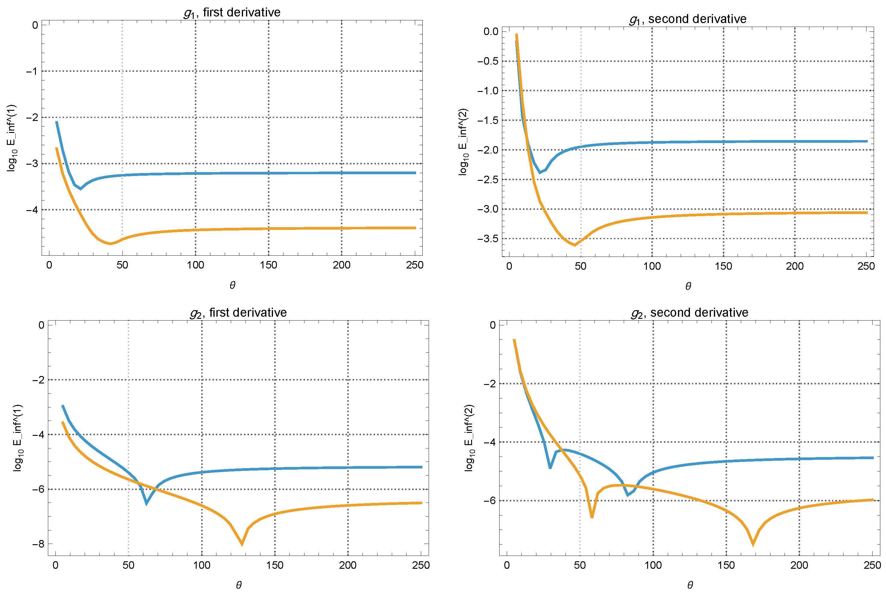
To illustrate the shape-parameter sensitivity, we plot the error curves

$$\theta \mapsto E_{\infty }^{\left(1\right)}\left(\theta \right),\theta \mapsto E_{\infty }^{\left(2\right)}\left(\theta \right),$$

for the two smooth test functions $g_1$ and $g_2$. In these tests, the nonuniform mesh (77) is used with $\delta =0.1$, and the shape parameter is written in the local form

$$c=\theta h.$$

The computations are performed for $N=80$ and $N=160$, and the results are displayed in Figure 1. The vertical axis is shown on a logarithmic scale in order to reveal the accuracy variation over the whole tested interval of $\theta$.

Figure 1 shows that the accuracy of the MQ RBF–HFD formulas depends noticeably on the shape ratio $\theta$. For both test functions and both grid sizes, the error curves exhibit an interval of favorable values of $\theta$, rather than a single universally optimal choice. Very small values of $\theta$ correspond to sharply varying MQ basis functions relative to the local mesh spacing and may increase the local truncation error. Very large values of $\theta$ move the method toward the flat-shape regime, where the weights approach their compact FD limits, but the underlying MQ Hermite systems become increasingly ill-conditioned. The observed curves therefore support the use of the combined diagnostic (79) and the selection rule (80), which balance accuracy, conditioning, and Fourier-resolution effects.

8. Conclusions and Future Work

In this paper, the analysis showed that the MQ RBF–HFD weights possess a compact structure that can be interpreted through the general local formulation (44). Their uniform-grid limits recover compact finite-difference-type formulas, while the local Fourier symbols provide insight into the effects of mesh nonuniformity and the shape ratio $\theta =c/h$. The shape-parameter criterion (69) further clarifies the balance between truncation error, conditioning, and spectral resolution.

Future work may extend the present analysis to wider compact Hermite stencils, multidimensional scattered nodes, and irregular domains. Another important direction is the development of adaptive mesh refinement strategies guided by the local truncation-error, conditioning, and Fourier-resolution indicators introduced in this paper. It would also be useful to investigate hybrid MQ–PHS compact formulations, which may combine the explicit accuracy of shape-dependent MQ weights with the robustness of shape-parameter-free PHS-polynomial augmentation. Finally, stabilized implementations based on scaling, preconditioning, or extended precision should be considered for strongly nonuniform meshes and highly ill-conditioned local Hermite systems.