Article

Lie Symmetries as a Mathematical Methodology to Identify Conservation Laws in Physiological Systems


by
Alice De Carli
1,2 and
Matteo Barberis
1,2,3,*
1
Molecular Systems Biology, School of Biosciences, Faculty of Health and Medical Sciences, University of Surrey, Guildford GU2 7XH, Surrey, UK
2
Centre for Mathematical and Computational Biology (CMCB), University of Surrey, Guildford GU2 7XH, Surrey, UK
3
Immunology, School of Biosciences, Faculty of Health and Medical Sciences, University of Surrey, Guildford GU2 7XH, Surrey, UK
*
Author to whom correspondence should be addressed.
Symmetry 2026, 18(7), 1143; https://doi.org/10.3390/sym18071143
Submission received: 25 April 2026 / Revised: 26 June 2026 / Accepted: 1 July 2026 / Published: 4 July 2026
(This article belongs to the Special Issue Integral/Differential Equations and Symmetry)

Abstract

Systems Medicine aims to understand the dynamics of physiological systems and the differences between healthy and disease states, to then bring the latter back to health. To this aim, it is critical to identify the states that allow modifying the phenotype of a model system and are robust to perturbations. Indeed, for these changes to be sustained in time, the system’s robustness shall be investigated through various analyses and their emerging results. Lie symmetry analysis—a study of fixed variable relations in a differential equations model—uncovers the model’s hidden robustness through its conservation laws. The emerging conservation laws can then be used as a series of robust invariant characteristics of the system under a specific type of perturbations. Although it holds much predictive potential for robustness investigations, the application of Lie symmetry-based conservation law analysis to physiological systems is currently unexplored. Here, we propose a novel application of Lie symmetry-based conservation law analysis to identify the conservation laws—and their existence conditions—influencing the dynamics of a system towards robust remission or relapse. This methodology is used to analyse a minimal model of rheumatoid arthritis with the aim to: (i) investigate the existence and extent of robust disease characteristics as conservation laws of the model, (ii) clinically interpret their biological viability, and (iii) inform model plausibility, testing, and selection. This novel application of the Lie symmetry analysis can retrieve the robust characteristics of physiological conditions, thus providing a new analytical contribution to the Systems Medicine field.

1. Introduction

Complexity in biological systems arises from the many molecules and mechanisms that allow such systems to express and maintain their functions. Physiological systems and their molecules are subject to naturally occurring perturbations, stemming from either mutations, environmental variations, or random fluctuations in the biochemical concentrations under scope [1]. Robustness plays an important role in such complex functional interplay [1,2,3], allowing a biological system to maintain its functionalities, despite being subject to both internal and external perturbations [3]. Indeed, a system whose state is not changed despite perturbations is called robust [1]. Robustness is widely encountered both in physical and biological systems [2,3]. For instance, in the budding yeast cell cycle, definite structural network motifs maintain their robust oscillatory behaviour under perturbations, therefore correctly ensuring cell differentiation [4,5]. Therefore, it is possible to investigate molecular mechanisms underlying cell cycle dysregulation as a proxy to understand cellular oncogenesis. Thus, investigating the robustness of biological systems allows for a better assessment of their functions by either resisting or adapting to perturbations. In the context of physiological systems, investigating robustness is key to gaining rich insights into how health and disease states adapt to treatment-like perturbations, therefore opening the floor to hypotheses of therapeutic treatment in silico. The first step towards the in silico study of a physiological system’s robustness is its formal description, to allow accurate analyses to be performed [4,6,7,8].
Systems Medicine addresses physiological systems and their functionalities, also in terms of robustness of networks arising among their components, with the aim to investigate disease dynamics and identify possible therapeutic interventions. Mathematical-based tools are needed to precisely investigate the structure and dynamics of such physiological systems [6,7,8]. Dynamical models are used to formally study complex physiological networks that are not fully understood [7,8], also in terms of their robustness [1,2,9]. Dynamical physiological models allow for the investigation of both the pathogenesis and pathophysiology of disease conditions, alongside any common underlying disease mechanisms. For instance, complex physiological networks can describe individual tumoural [10,11,12,13] and autoimmune disorder [7,14,15,16] dynamics, alongside possible interactions between them [17,18,19].
Analysing robustness trends in dynamical physiological models is key to understanding health and disease mechanisms for many in silico conditions of interest [1,2,3]. For instance, robustness analyses help address disease heterogeneity [6]. The course and prognosis of the same disease are inconsistent and largely vary among patients because both genetic and environmental factors play an important role in disease onset [7,20]. Studying robustness in in silico physiological network models enables the prediction of how an ad hoc physiological system will react and adapt to different induced treatment-based stimuli. Analysing the personalised system’s robustness response will enable a deeper understanding of the response a patient might potentially undergo upon personalised treatment [21,22]. Robustness analyses also allow investigating how treatment-induced disease states changes are maintained in time. Therefore, when engineering personalised treatment, a change from a disease state to health maintained in time will be favoured over a temporary change, which will possibly require further treatment-based stimuli to be sustained [21,23]. Numerous dynamical models exist that address disease heterogeneity and investigate personalised treatment in physiological systems by altering the environmental conditions and testing drugs as input. One such example is the study of the dynamics of different disease stages in Systemic Lupus Erythematosus (SLE) in terms of tissue-level and systemic inflammation, for different naturally occurring and treatment-based stimuli [7,14]. Finally, robustness analyses allow for the validation and evaluation of dynamical models [24,25,26]. Building a dynamical model includes choosing between alternative representations of the same qualitative behaviours featured in the system’s phenotypical landscape [25]; in this context, robustness analyses allow distinguishing between more and less plausible models by comparing clinical and experimental evidence with the robust behaviours exhibited. Therefore, by studying which robustness principles a model obeys, it is possible to refine existing dynamical models and possibly build new ones that better describe the mechanisms under investigation [24,25].
In summary, analysing robustness in physiological dynamical systems is key to fully utilising their predictive power in investigating disease and health mechanisms under varying conditions, as well as in testing novel treatment hypotheses in silico. Moreover, from a modelling perspective, robustness insights could pave the way towards a more precise mathematical reproducibility of the clinical and experimental evidence on a condition of interest via modelling evaluation and validation. However, while significantly rich, studying robustness in dynamical physiological models is not straightforward and needs to be performed through structured and precise analytical techniques, whose development field is still currently growing [1,2,3,25].
Differential equations (DEs) are widely used to investigate how dynamical systems behave as one or more of their variables change and, by extension, how robustness arises in their adaptation mechanisms to perturbations [27,28]. DEs can inform how biochemical quantities or concentrations in a system evolve in time and space, thus enabling the analysis of their time- and space-dependent behaviour. Different types of DEs can be used in dynamical modelling. Ordinary Differential Equations (ODEs) inform how a system evolves in time, thus allowing to analyse its time-dependent behaviour. To do so, ODEs incorporate time-dependent derivatives of the dependent variables in the system [8,28]. Indeed, ODEs have been used to model the temporal evolution of cell-cycle kinetics [4] and interacting cell populations [16].
Robustness in ODE models can be analytically analysed through various available tools [27,28]. Among these, conservation laws allow studying a system’s robustness in terms of its structure and internal mechanisms [2,29]. Conservation laws allow for the analytical identification of quantities or relations that do not change—thus, that are robust—under different types of perturbation [29,30,31]. For instance, a conservation law arising in closed-population Susceptible–Infected–Recovered (SIR) models accounts for the unchanging total number of individuals in the system, thus supporting robustness to changes in the total population number—with the same dynamics being reproduced irrespectively of the total population number assumed and of its possible fluctuations [26].
The conservation laws of a DE model—and therefore of an ODE model—can be derived through Lie symmetry analysis. In simple terms, a symmetry is a transformation that, when applied to an object or a system, leaves something unchanged [26,32]. In DEs, a Lie symmetry is a transformation of a model’s variables preserving its solutions [32]. Therefore, Lie symmetry analysis can be useful in model simplification, evaluation and analysis [24,26,33]. Lie symmetries are linked to conservation laws by Noether’s theorem [34], which allows the use of Lie symmetry analysis-based methods to find the conservation laws of a DE model [29,35]. The Lie symmetry-based analysis of conservation laws via Noether’s theorem has been implemented in various biological systems, such as genomics [36] and population studies [37], but is still widely unexplored in physiological systems of health and disease.
In this study, a Lie symmetry-based conservation law analysis is proposed as a novel approach for systems biology and medicine to gain insights on the robustness of physiological disease systems. While conservation laws are widely applied in scientific fields other than biology [29,30,38], their application for robustness investigation in disease and health models is currently unexplored. The discussed methodology involves an original investigation of a physiological system’s structure in terms of a set of formally derived analytical conditions. Such conditions are found to be expressed in terms of variables and experimentally based parameters augmented in the disease model. The proposed Lie symmetry-based conservation law analysis could, therefore, potentially be applied to a range of patient-specific clinical parameters towards the prediction of in silico personalised treatment approaches. Therefore, this study aims at paving the way towards the analytical application of Lie symmetry-derived conservation laws to retrieve the robust characteristics of a physiological condition of interest in terms of its mathematical model’s structure—thus providing a new analytical contribution to the Systems Medicine field. As a clinical case study, the proposed analysis is conducted on the mathematical model of cytokine-mediated inflammation in rheumatoid arthritis (RA) [16], an autoimmune disorder.
Autoimmune disorders affect approximately 10% of the global population [7,39] and are characterised by an abnormal response of the immune system in a patient’s body, usually through inflammation [7]. Currently, it is often possible to achieve drug-dependent remission in about 30% of the population affected by autoimmune diseases [40]. However, once a drug is withdrawn due to the unfeasibility of maintaining a drug treatment indefinitely, only between 10% and 20% of patients maintain remission [40]. Thus, about 50% of the patients with drug-dependent remission maintain drug-free remission, while the remaining 50% fall into relapse (see Figure 1). Therefore, it appears to be critical to analytically investigate drug-free remission so that it becomes achievable for all patients [21].
Rheumatoid arthritis (RA) is a chronic, systemic autoimmune disease affecting 1% of the UK population [41], with symptoms such as prolonged pain, inflammation, swelling and stiffness in the joints, as well as whole-body tiredness and high temperatures [41,42]. This persistent joint inflammation, both in the bone and cartilage tissues, progressively leads to joint destruction and, if left untreated, disability and early death [7,20,41]. In particular, the synovium in a patient’s joints experiences synovial hyperplasia, a condition where the layer of cells lining the joint capsule—also known as the synovial lining cells—proliferates [7]. This aberrant proliferation leads to an inflammatory response [16] mediated by the recruitment of both adaptive and innate immune cells to the inflamed site, here the synovium, partly via the production of cytokines [43,44,45,46]. Cytokines are important cellular signalling proteins and immune system mediators secreted and released by cells upon inflammation [46], kickstarting a series of defence mechanisms, thus activating various cellular responses to infection and injury [43]. Dysregulation in the production of inflammatory cytokines is largely associated with autoimmune diseases, such as RA [16,38,43,47]. In RA progression, the imbalance between pro- and anti-inflammatory cytokines—caused by an aberrant concentration of pro-inflammatory cytokines—is key to synovial hyperplasia [41,42,48,49,50,51]. A large range of cytokines has been identified in the synovium during RA onset, both clinically and experimentally, modulating the severity and the duration of the associated inflammation [38,47,52]. Among them are the pro-inflammatory cytokines Interleukin-1 (IL-1) and Tumour Necrosis Factor- α (TNF- α ) [38,42,44,48,51], and the anti-inflammatory cytokines IL-1 Receptor antagonist (IL-1Ra) and Interleukin-10 (IL-10) [38,45,47]. Pro- and anti-inflammatory cytokines interact with each other within an activator/repressor relationship [43,53,54]. Indeed, the pro-inflammatory cytokine TNF- α upregulates both its own production and that of other pro-inflammatory cytokines [42,48,51,55]. Moreover, TNF- α upregulates the production of the anti-inflammatory cytokine IL-10, thus acting as its activator. At the same time, IL-10 upregulates IL-1 Receptor (IL-1R), another anti-inflammatory cytokine, and acts as a repressor by downregulating TNF- α [38,53].
Mathematical modelling and robustness analysis of RA dynamics can help to elucidate its disease mechanisms, as well as informing decision-making within treatment administration and development [7,16]. Indeed, dynamical modelling allows studying RA dynamics at multiple spatial scales, such as the molecular, cell and joint levels [41]. For instance, a two-variable ODE model of RA [16], referred here to as the “Baker model”, has been used to describe and study the dynamics of pro- and anti-inflammatory cytokines within the inflamed synovium at the cell level via intracellular interactions [16,41]. Hill equations are embedded into the Baker model to integrate an activator/repressor dynamic [56,57], as per the experimental evidence of the interactions among pro- and anti-inflammatory cytokines [43,53,54]. The cytokine dynamics emerging from the Baker model stem from the interactions within the system and with the surrounding environment [16]. Thereafter, the authors studied RA’s heterogeneity and robustness to naturally occurring and treatment-based perturbations through the investigation of the cytokines’ dynamics in their parameter space [16]. However, the conservation laws regulating the cytokine RA-inflamed synovium system were not explored, therefore giving a partial view of the overall robustness. Indeed, the multiple behaviours observed in the pro- and anti-inflammatory cytokines’ parameter space investigated allow for the systematic classification of various model behaviours, which can then be further investigated in terms of the system’s conservation laws.
In this study, the proposed novel Systems Medicine application of Lie symmetry-based conservation law analysis is tested on the Baker model of RA to assess the system’s robustness not only in terms of its temporal dynamics, as published in [16], but also with respect to its structure-based conservation laws regulating the RA-inflamed synovium system. The aim of this case study is to uncover any robust characteristics of the Baker RA system that remain hidden in a traditional dynamics study of the model, but that can potentially be found via the novel application of a structural Lie symmetry-based conservation law analysis. Thus, a conservation law with respect to time—also known in the literature as “conservation of energy” and likened to experimental reproducibility [36,58]—emerges from the Baker model for a set of parametric conditions of validity. This conservation law is then linked via clinical and experimental evidence to the emergence of inflammation flares in RA [42,59,60,61], in particular to their unfeasible coexistence in one same disease phenotype. This insight is then used to shed light on (i) inflammation flare robustness and (ii) model evaluation and selection for the Baker model. Lastly, the proposed Lie symmetry-based methodology is argued to hold potential in paving the way towards a quantitative and potentially personalised modelling for RA patients—and more widely for other similar autoimmune disease models. In conclusion, the proposed original application of Lie symmetry analysis to the RA Baker model allows gaining novel analytical information on the onset of disease phenotypes of interest, and to further discuss the optimisation of the mathematical in silico representation of inflammation dynamics.

2. Materials and Methods

2.1. Definition of the Baker Model

The general form of the 2013 Baker et al. [16] two-variables Ordinary Differential Equations (ODEs) model
d p d t = d p p + ϕ ( p ) θ ( a ) d a d t = d a a + ψ ( p )
investigated in this paper describes the dynamics of pro- and anti-inflammatory cytokines in the synovium during rheumatoid arthritis (RA) progression, respectively described by the p ( t ) and a ( t ) time-dependent variables. The two ODEs in Equation (1) represent the change in time of both cytokines’ concentrations—mathematically described by the two derivatives with respect to time, d p d t and d a d t —via two terms:
  • The linear, natural degradation terms of both cytokines, scaled by the two pro- and anti-inflammatory cytokine-specific factors d p and d a , respectively;
  • The interaction terms between cytokines, modulated by the functions ϕ ( p ) , θ ( a ) and ψ ( p ) , which can be chosen depending on the specific type of cytokines’ dynamics and cytokine–cytokine interactions of interest.
Equation (1) assumes that all cytokines in the synovium have similar response patterns, thus considering the synovium as a spatially homogeneous collection of cells. Moreover, the model neglects other cytokines’ functions other than their natural degradation and cytokine–cytokine interactions, such as cytotoxic mechanisms [16,41].
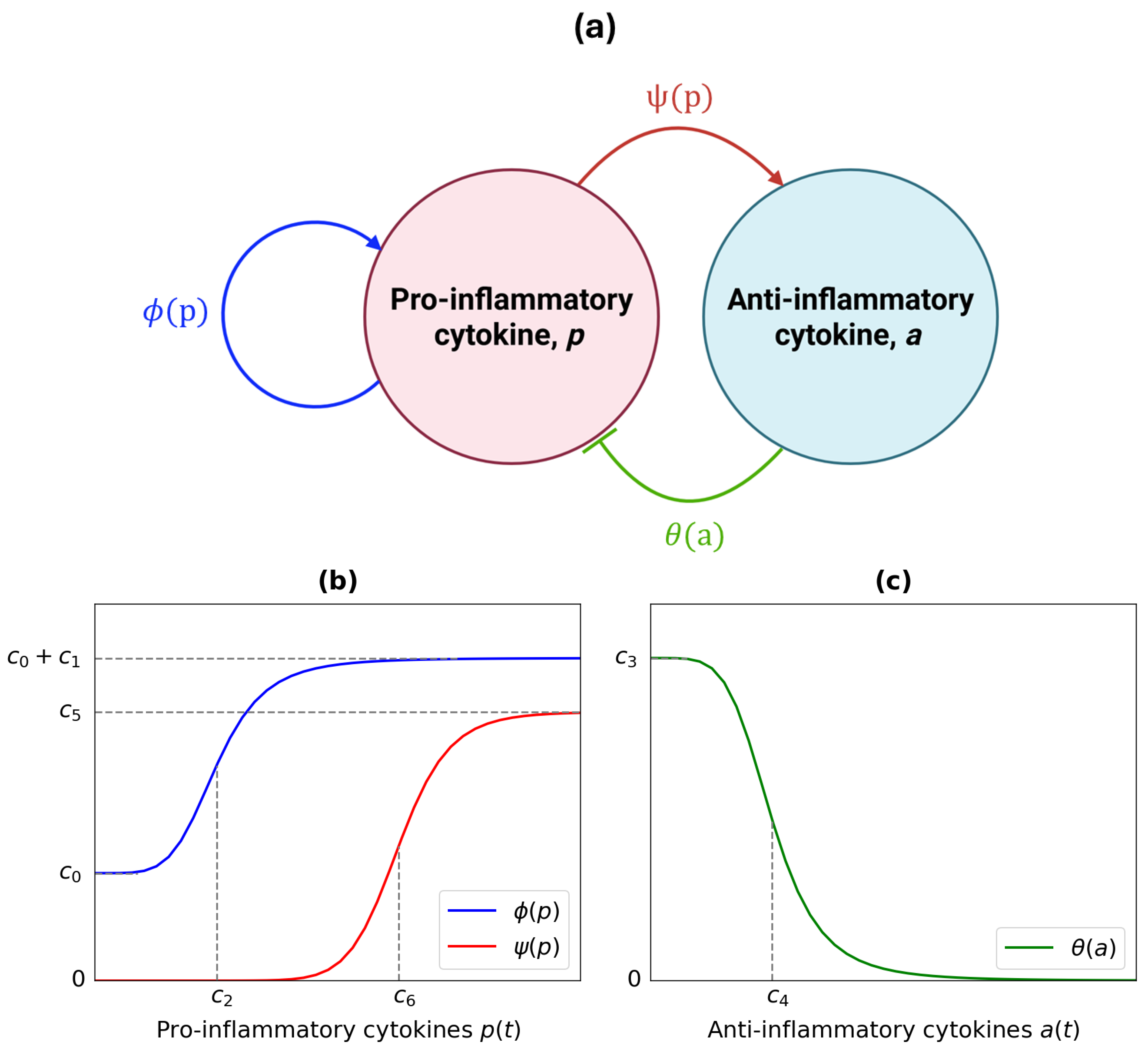
The generalised model in Equation (1) can be further defined by explicating its interaction terms [16], thus integrating some specific type of cytokine–cytokine interaction dynamics of interest. As previously discussed, experimental evidence shows that pro- and anti-inflammatory cytokines follow an activator/repressor relation on one another [16,43,53,54,55]. Consequently, embedding the Hill equations
ϕ ( p ) = c 0 + c 1 p m 1 c 2 m 1 + p m 1 θ ( a ) = c 3 c 4 m 2 c 4 m 2 + a m 2 ψ ( p ) = c 5 p m 3 c 6 m 3 + p m 3
qualitatively plotted in Figure 2 allows integrating the pro- and anti-inflammatory cytokines’ activator/repressor interactions within the model’s structure [56,57].
As a result, the dimensional model
d p d t = d p p + c 0 + c 1 p m 1 c 2 m 1 + p m 1 c 3 c 4 m 2 c 4 m 2 + a m 2 d a d t = d a a + c 5 p m 3 c 6 m 3 + p m 3
arises, where [16]:
  • c 0 , c 1 , c 2 , c 3 , c 4 , c 5 , c 6 > 0 are some constant parameters. c 0 is the basal pro-inflammation cytokines’ production rate. The 2013 Baker et al. [16] model assumes some level of inflammation to always be present in the synovium system. Therefore, c 0 > 0 allows for a basal concentration of inflammation-inducing pro-inflammatory cytokines to always be active in the system, and thus inflammation to always be included; c 1 describes the additional pro-inflammatory cytokines’ production rate due to their self-upregulation at the p saturation maximum concentration; p = c 2 is the half-maximal concentration point for the self-upregulation in pro-inflammatory cytokines’ dynamics; c 3 describes the basal inhibitory effect in the absence of anti-inflammatory cytokines; a = c 4 is the half-minimal concentration point for the pro-inflammatory cytokines’ downregulation due to the anti-inflammatory cytokines; c 5 describes the maximal activator effect of pro-inflammatory cytokines on anti-inflammatory cytokines within anti-inflammatory cytokines’ dynamics; and p = c 6 is the half-maximal concentration point for the upregulation of anti-inflammatory cytokines by pro-inflammatory cytokines within anti-inflammatory cytokines’ dynamics.
  • m 1 , m 2 , m 3 are the Hill coefficients modulating the strength of the activator/repressor responses within the pro- and anti-inflammatory cytokines’ interactions. Graphically, a larger Hill coefficient will correspond to a steeper Hill function curve in Figure 2 and vice versa.
Thanks to the Hill functions ϕ ( p ) , θ ( a ) and ψ ( p ) , the dimensional model in Equation (3) effectively describes the activator/repressor cytokines’ interactions discussed. Indeed, ϕ ( p ) and ψ ( p ) contribute positively to the growth of both pro- and anti-inflammatory cytokines, thus reflecting the activator role played by pro-inflammatory cytokines. At the same time, θ ( a ) interacts with ϕ ( p ) by hindering pro-inflammatory cytokines’ growth, consequently showing anti-inflammatory cytokines acting as repressors within the cytokines’ interactions.
To more easily investigate the dynamics yielded by Equation (3), Baker and colleagues [16] perform a nondimensionalisation on the model, reducing the number of parameters by defining new dimensionless ones. Indeed, the use of dimensionless variables and parameters allows for an easier assessment of model features, such as term sizes and physical mechanisms, and can potentially simplify the equations by taking care of negligible terms [62,63,64]. To perform a nondimensionalisation, all variables in the model are first defined in terms of their characteristic scales and their dimensionless factors. A characteristic scale is a reference value used to normalise the dimensional variable, thus to define a dimensionless factor. In general, there is no unique way to perform this step and the choice of characteristic scales is usually informed by the scientific literature on the known system’s characteristics [62,64]. Thus, the emerging
d p d t = γ p + 1 1 + a m 2 α 1 + α 2 p m 1 1 + p m 1 d a d t = a + α 4 p m 3 α 3 m 3 + p m 3
nondimensionalised model arises, where its dimensionless parameters are interpreted as [16]:
  • α 1 = c 0 = c 0 c 3 c 2 d a is the basal pro-inflammatory cytokines’ production rate;
  • α 2 = c 1 = c 1 c 3 c 2 d a is the additional pro-inflammatory cytokines’ production rate thanks to their self-upregulation;
  • α 3 = c 6 d a c 3 = c 6 c 2 is the pro-inflammatory cytokines’ concentration for half-maximal anti-inflammatory cytokines’ production;
  • α 4 = c 5 c 4 d a is the anti-inflammatory cytokines’ production rate;
  • γ = d p d a is the ratio between the pro-inflammatory cytokines’ degradation rate d p and the anti-inflammatory cytokines’ degradation d a .
In Baker et al. (2013) [16], the dimensionless parameters α 1 , α 3 and γ are determined by both the size and structure of the cytokines and the chemical environment within the host. Therefore, in a patient, these parameters are assumed to remain either fixed or changing at a much larger timescale in a patient compared to the inflammation-dependent parameters α 2 and α 4 . In particular, according to the authors [16]: (i) α 1 < < α 2 , as the background level of pro-inflammatory cytokines p production is assumed to be much smaller than the event-stimulated production α 2 . This relation between α 1 and α 2 allows the model to reflect an effective response to infection and injury; (ii) α 3 = c 6 c 2 is expected to be of order one, as the half-maximal p concentrations for both self-upregulation ( c 2 ) and a upregulation ( c 6 ) are argued to have reasonably similar values to reflect a downregulation of p; and (iii) γ = d p / d a 1 , as the two degradation rates d p and d a are argued to be similar.
Another step to further define the model in Equation (4) is choosing a value for its Hill coefficients m 1 , m 2 and m 3 [16]. This choice will modulate the strength of the activator/repressor relationship between the pro- and anti-inflammatory cytokines in the RA-inflamed synovium [16,57], thus affecting both the cytokines’ concentrations and the disease’s evolution in time. This selection is informed by a series of dynamics investigations performed on different adaptations of Equation (3) for various m 1 , m 2 , and m 3 values [16]. Therefore, the best model according to the published results has m 1 = m 2 = m 3 = 2 , since:
  • m 1 = m 2 = m 3 = 1 restricts the range of behaviours allowed by the model. In particular, m 1 = 1 prevents bifurcations and bistability from arising.
  • The two cases where m 1 > 1 (here m 1 = 2 for simplicity), m 2 = m 3 = 1 or m 2 = m 3 = 2 both allow a wider range of qualitatively equivalent behaviours to show compared to m 1 = m 2 = m 3 = 1 . However, for m 2 = m 3 = 1 , the equilibria tend to arise for larger concentrations of p and a, and are thus deemed less favourable for computational ease.
  • For m 1 , m 2 , m 3 > 2 , the shapes of the Hill functions do not change, but only their steepness does. Consequently, adopting m 1 , m 2 , m 3 > 2 does not widen the range of possible behaviours while formally complicating the model.
Following these results, the m 1 = m 2 = m 3 = 2 Hill coefficients are substituted into Equation (4) to recover
d p d t = γ p + 1 1 + a 2 α 1 + α 2 p 2 1 + p 2 d a d t = a + α 4 p 2 α 3 2 + p 2 .
Thereafter, the authors in Baker et al. (2013) [16] use Equation (5) to investigate different RA expressions and hypothetical treatment strategies through the evolutionary dynamics of pro- and anti-inflammatory cytokines.
In this study, the nondimensionalised and Hill coefficient-integrated model in Equation (5)—which will be referred to from here onwards as the “Baker2013 model”—will be used as the case study for cytokines’ dynamics in the RA-inflamed synovium. Indeed, it gives a wide range of phenotypical behaviours previously investigated by Baker and colleagues [16] that can be further studied via the proposed Lie symmetry analysis.

2.2. Lie Symmetries and Conservation Laws

In simple terms, a symmetry is a transformation that, when applied to an object or a system, leaves something unchanged [26,32]. For instance, the geometrical symmetry of an object is a transformation that preserves its structure. In general, symmetries are a fundamental aspect of many laws of nature, and they can often be encountered in everyday life. Take, for example, the shapes of butterflies and human bodies in nature, which both show geometrical bilateral symmetry. Art and architecture also often feature geometric symmetric characteristics, albeit man-made, such as mirrored facades or repeated patterns of columns and arcs.
Symmetries are not solely confined to their everyday qualitative instances. In the mathematical study of biological systems, symmetries allow for the analysis and the exploitation of the inherent regularity found in many such systems [65]. Indeed, symmetries can be used in various problems to ease their investigation [32]. In the context of modelling biological systems, geometrical symmetries can often be noticed straightforwardly and thus be easily exploited [32,33]. As an example, let us consider a tumour spheroid model [66]. First, geometrical symmetries will be found by observing the spheroid. Indeed, a series of rotations about its centre will be identified, such as 2 π , that leave the spheroid unchanged. Thereafter, it is possible to use this symmetrical characteristic to simplify the mathematical form of the tumour model under study. In particular, the spherical symmetry of tumour spheroids will allow the investigator to perform a change of variables (from Cartesian to spherical polar coordinates), which will then ease the emerging dynamics under investigations [66].
In mathematical modelling, symmetry analysis can also be extended to study the properties of Differential Equations (DEs) [26,32,67]. Symmetries applied to DEs are called Lie symmetries [26,32,67]. The origins of Lie symmetries trace back to the 19th century, when the Norwegian mathematician Sophus Lie first began to investigate the application of invariant transformations to DEs [65,68,69]. To explain what an invariant transformation is, we shall go back to the first qualitative definition of symmetries. As just discussed, a symmetry in general is an operation that leaves something unchanged [26]. This qualitative definition of symmetry can be mathematically formalised via the introduction of invariance. An object can be described as invariant under a certain transformation when such an operation leaves it unchanged. Applied to the original definition of symmetry, it can be said that an object has at least one symmetry when it is invariant under some transformation. By extension, it can thus be said that a symmetry applied to a certain system or object is an invariant transformation, when it leaves such object or system invariant, i.e., unchanged [26,33,65].
A practical example can be used to better understand what an invariant transformation is. Let us say we want to study the spread of an infectious disease in a population. It is assumed that each individual is initially susceptible to the disease, can get infected and can recover, thus gaining immunity. Moreover, it is assumed that the total population N remains constant; thus, births, immigration, emigration, and deaths are not included in this study, i.e., the population is closed. Such a scenario can be modelled via an ODE Susceptible–Infected–Recovered (SIR) model, an approach that has been widely used in mathematical epidemiology to successfully study a wide variety of contagious diseases, such as coronavirus disease 2019 (COVID-19), in a defined time window [26,70,71]. Even before formally analysing the SIR model mathematically, some observations can be made based on the qualitative understanding of the problem at hand. For instance, it can be said that no matter the exact point in time when the disease starts spreading, the infection dynamics will stay the same. In other words, no matter whether the first infected case appears (for example, today or in a month’s time), the way the disease spreads within the population will remain largely the same. Another observation is that the recovered population does not influence the spread of the disease. Indeed, it is known from the assumptions that once a person recovers, they cannot get re-infected, and thus can no longer contribute to the disease spread [70,71]. What these observations imply is that no matter the conditions imposed on the model, as long as the current assumptions hold, neither the initial infection time-point nor the recovered population number will influence the infectious dynamics of the disease. From a mathematical point of view, it can thus be said that the dynamics of the disease spread will be (i) invariant under time translations, and (ii) invariant under translations within the recovered population [26]. Now, let us move one step further in the SIR example and assume we want to study a more mathematically complex SIR model. Let us say that the previous modelling assumptions still hold, specifically that the total population N is conserved and that each recovered individual does not revert to a susceptible state. Let us also assume that the mathematical form of the SIR model is now considerably more complex to analyse compared to the first example, and would thus be more challenging to solve analytically and computationally. Nonetheless, the definition of invariant transformations as unchanging identities characterising a system allows observing that the disease spread will still be invariant under both time and recovered population translations without having to explicitly solve the now more complicated SIR model.
Let us now look at invariant transformations in the context of Lie symmetries. In the scientific literature, Lie symmetries are often referred to as just “symmetries” when the research analysis is performed around a DE or a DE system. Thus, in this paper, the terms “symmetry” and “Lie symmetry” will often be used interchangeably. Often, the equations describing a DE model can be simplified by changing its variables via a specific manipulation. This simplification principle was previously discussed in the tumour spheroids models’ example, where a change from Cartesian to spherical polar coordinates has been shown to significantly ease its investigation [66]. Finding a fit manipulation for an effective change of variables can, however, be potentially challenging. Symmetries can help in making this change-of-variables choice [26]. In particular, manipulation of variables arising from a symmetry study can transform both the dependent and independent variables of a DE model. This symmetry-informed manipulation results in a formally new, simpler DE model that reproduces the same result as the original model [26,32,67]. Formally, it can be said that this new DE model is a Lie symmetry to the original model if the applied transformation is invariant. In other words, a Lie symmetry can be found if the new DE solution set maps to the original one [26,32,67]. To better understand the implications of Lie symmetries and their connection to translational invariants, let us go back to the SIR example. It is known that, for a specific set of assumptions, the SIR model will yield at least two invariant translations, respectively concerning time and the recovered population number [26]. Thus, this result can be used to identify a change of variables which will (i) simplify the SIR model and (ii) involve the time and/or the recovered population variables. In particular, through Lie symmetry analysis, a particular variable simplification—i.e., a Lie symmetry—can be found that allows retrieving, from the solution set of the more complicated SIR model, the solution set of a simpler model [24,26,32].
Model simplification is not the only application of Lie symmetries in dynamical modelling. More specifically, Lie symmetries can help uncover the conservation laws of a model under study [2,26,37,65,67,72,73,74]. Conservation laws are powerful constraints in the dynamics of many systems present in nature [29,30,31] because they allow for the identification of some quantities or relations in a dynamical system which do not change under different types of perturbation. Their identification provides insights into the system’s dynamics and a means for the simplification of the model’s form [29,30,31]. For instance, a commonly known conservation law is the conservation of energy, stating that energy in an isolated system can never be created or destroyed but only transformed [58]. The conservation of energy has been successfully used to investigate various systems, such as early-cell metabolic pathways [75], physiologically structured population models [76] and respiratory circuits [77]. Conservation laws and Lie symmetries are tightly interconnected via Noether’s theorem [29,36,37,65,67]. First formulated in 1915 by Emmy Noether in the context of calculus of variations [34], Noether’s theorem aims to identify invariant transformations called “Noether’s symmetries” [35,36]. In its less rigorous formulation, Noether’s theorem states that every Lie symmetry held in a physical system has a corresponding conservation law [36]. In other words, a DE system admitting a Lie symmetry algebra will also allow for one or more conservation laws, which can be derived via Lie analysis. Noether’s theorem has been successfully applied to link conservation laws and symmetries to both physical and biological systems [36,37,65], for example to population models [37] and genomics [36] to discuss their arising conservation laws. To better understand how Noether’s theorem comes into play and its relationship with Lie symmetries, let us once again take the SIR model example above, and perform a three-step analysis towards the identification of its conservation laws [37]: (i) compute the Lie symmetries of the model, (ii) find the respective invariants, and (iii) identify their conservation laws. Earlier, the SIR model was discussed to be (i) Lie symmetric with respect to time and, thus, (ii) invariant to time translations [26]. Noether’s theorem then allows (iii) identifying a conservation law linked to the time translation, here energy conservation [26,36,58]. Another conservation law of the SIR model can be identified using the closed population assumption. As per the above assumption, no births, immigrations, emigrations, or deaths occur within the SIR model. Mathematically, this assumption can be expressed by augmenting the N = S + I + R equation into the SIR model, where N is the total population, and S, I and R are the susceptible, infected and recovered populations, respectively [26]. Via Lie analysis, it is then possible to (i) find, i.e., a Lie symmetry defining (ii) N as an invariant of the model. Then, Noether’s theorem [34,36] allows identifying (iii) the mass-conservation law of the SIR model [26].
To better solidify and correctly use the Lie symmetry and conservation laws concepts that have been qualitatively discussed, some mathematical formalism will now be introduced.
Definition 1.
R σ [ u ] is a system of N k-th order ODEs if
R σ [ u ] = R σ ( x , u , u , , k u ) = 0 , σ = 1 , , N ,
for one independent variable x X and m dependent variables u u ( x ) = u 1 ( x ) , , u m ( x ) U [72,73].
In Equation (6), the set of all partial derivatives p u of order p = 1 , , k of the m dependent variables u = u ( x ) with respect to the independent variable x is defined as
p u = p u μ ( x ) x p | μ = 1 , , m = u p μ | μ = 1 , , m U p , p = 1 , , k
for u ( x ) = u 1 ( x ) , , u m ( x ) [73].
Definition 2.
The total derivative D of the m dependent variables u u ( x ) = u 1 ( x ) , , u m ( x ) U with respect to the independent variable x is defined as the differential operator
D x = x + u μ x u μ , μ = 1 , , m ,
where it is implied that the repeated indices sum together [26,73].
Definition 3.
A Lie point symmetry can be defined as the variables transformation from the m dependent variables u u ( x ) = u 1 ( x ) , , u m ( x ) U with respect to the independent variable x—to the transformed variable set ( x ˜ , u ˜ μ ) , μ = 1 , , m —respectively described by the set of functions f and g μ as
x ˜ = f ( x , u , ϵ ) , ( u ˜ ) μ = g μ ( x , u , ϵ ) , μ = 1 , , m ,
which can be written in its local form as
x ˜ = x + ϵ ξ ( x , u ) + O ( ϵ 2 ) , ( u ˜ ) μ = u μ + ϵ η μ ( x , u ) + O ( ϵ 2 ) , μ = 1 , , m
where ϵ I R parametrises the curve connecting each original solution of the system R σ [ u ] to its Lie-transformed equivalent [26,72]. Equation (10) is the Taylor series to the first order in ϵ for the Lie group transformation in Equation (9), where the O ( ϵ 2 ) terms group together all higher-order terms of the series.
In Equation (10), the functions ξ ( x , u ) and η μ ( x , u ) act as individual components of the vector connecting the set of points to which the ( x , u μ ) , μ = 1 , , m variables can be mapped to by a suitable choice of ϵ and are defined as
ξ ( x , u ) = x ˜ ϵ ϵ = 0 and η μ ( x , u ) = u ˜ μ ϵ ϵ = 0 ,
for μ = 1 , , m [26,72].
Definition 4.
The Lie algebra of infinitesimal generators of symmetry, i.e., the Lie symmetry generator, for the k-th order ODE system R σ [ u ] in Equation (6) is defined as [26,73]
X = ξ ( x , u ) x + η 1 ( x , u ) u 1 + + η m ( x , u ) u m = ξ ( x , u ) x + η μ ( x , u ) u μ , μ = 1 , , m
where the functions ξ ( x , u ) and η ( x , u ) are the individual components of the vector field describing the variable transformation, as per Equation (11), considering m dependent variables u u ( x ) = u 1 ( x ) , , u m ( x ) U with respect to the independent variable x.
Definition 5.
Consider the transformations performed by some Lie algebra of infinitesimal generators of symmetry G, defined as per Definition 4. Then, in general, the action of G on a manifold Ω p is given by a differentiable map Γ : G × Ω p Ω p such that:
Γ g : ( x , u ) ( x ˜ , u ˜ ) ,
where g G is a fixed element of the Γ map, which will be referred to as a point transformation [26]—once again, considering m dependent variables u u ( x ) = u 1 ( x ) , , u m ( x ) U with respect to the independent variable x.
Definition 6.
A local invariant of the transformation group G, as defined in Definition 4, is a function I : Ω p I R such that
I ( Γ g ( x , u ) ) = I ( x , u ) ,
where the action of g G is described by the Γ map as per Definition 5 [26]—once again, considering m dependent variables u u ( x ) = u 1 ( x ) , , u m ( x ) U with respect to the independent variable x.
Definition 7.
A local conservation law of the k-th order ODE system R σ [ u ] in Equation (6) is the divergence expression
div Φ [ u ] D x Φ [ u ] = 0 ,
holding for all solutions of the ODE system. In Equation (15), D x is the total derivative with respect to the independent variable x as per Equation (8), Φ [ u ] = Φ ( x , u , u , , r u ) are known as the “fluxes of the conservation law”, and the order r of the highest-order derivative r in Φ [ u ] is known as the “differential order of the conservation law” [73].
In this study, the Lie symmetry concepts discussed here will be used to find the conservation laws emerging from the Baker2013 model in Equation (5). While the definitions above are needed to introduce the main theoretical notations and characteristics of Lie symmetries for k-th order ODE systems—as per the Baker2013 model—they are not going to be explicitly implemented in this paper. Indeed, the implementation of the computational tools presented below will allow deriving the conservation law trends of the Baker2013 model without explicitly going through the otherwise overly complex Lie symmetry analytical steps needed.

2.3. Computational Materials

Various computational techniques allow deriving the conservation laws for a system of k-th order ODEs, as per Definition 1 and Definition 7, without having to explicitly compute the Lie symmetry generators and the invariants of the model [72,73]. An example of a computational package enabling the production of such analysis is the Maple GeM software package for automated symmetry and conservation law analysis [72,73,78,79]. In general, the GeM package contains numerous powerful computational routines enabling the application of Lie symmetry and conservation law formalisms for different DE systems. Its appeal not only resides in the efficiency and accuracy of its analysis but also in the user-friendly symbolic approach it takes [72,78]. In particular, the GeM package can be used to seek the conservation laws of a DE model via four different methods, briefly described in Table 1.
In particular, the direct method uses local multipliers depending on both independent and dependent variables of the system. Then, the linear combination of the equations of the system, augmented with such multipliers, will give rise to a divergence expression for the fluxes of conservation laws of the form in Definition 7 [73].
In this study, the Maple GeM software package for automated symmetry and conservation law analysis is used to investigate the conservation laws governing the Baker2013 model in Equation (5). The computational analyses will be performed using the following tools’ versions: Maple 2024.2. Maplesoft, a division of Waterloo Maple Inc., Waterloo, ON, Canada [80,81]; and the GeM symbolic software package for general symmetry and conservation law analysis of differential equations, version 32.12 [72,73,78,79,82]. The implementation of the Maple software and the GeM package is fully reproducible, once set up as shown in the Maple script file in the Supplementary Material. Indeed, all Lie symmetry-based conservation law derivations performed in this study do not contain any non-deterministic, probabilistic or data-heavy element to them, which could potentially hinder both replicability and reproducibility. Therefore, all results of the GeM Maple package implementation found below and in the Supplementary Material—both partial and final—are fully reproducible. Moreover, the Eureka2 shared High-Performance Computing cluster, developed by the University of Surrey Research Computing Team (Guildford, UK), was used to breach local computing processing limitations, but its implementation does not influence the quality or the form of the results presented.

3. Results

In this study, the Lie symmetry methodologies discussed in Section 2.2 and Section 2.3 are used to assess how conservation laws arise in physiological systems of autoimmune disorders via a case study of rheumatoid arthritis (RA) [16], and how inflammation flares can be used as an indicator of biological feasibility.

3.1. Lie Symmetries and Conservation Law Analysis Preparation

The first step in the Lie symmetry and conservation law analysis of the Baker2013 model (Equation (5) [16]) is to rearrange its form so that it is optimal for its investigation. Let us begin by noticing that the model is a first-order Ordinary Differential Equations (ODEs) system. Definition 1 in Section 2.2 is used to define a system of N first-order ODEs
R σ [ u ] = R σ ( x , u , u ) = 0 , σ = 1 , , N ,
for one independent variable x and m dependent variables u u ( x ) = u 1 ( x ) , , u m ( x ) , where the set of all partial derivatives p u of order p = 1 , , k is defined in Equation (7) [72,73,83]. According to the scientific literature on Lie symmetries, all systems of first-order ODEs admit an infinite-dimensional Lie algebra of infinitesimal operators as in Definition 4 [32,37,84]. In other words, performing a Lie symmetry analysis on a system of first-order ODEs may potentially generate an infinite number of symmetries. Consequently, the derivation of both the Lie symmetry algebra and the conservation laws of a system of first-order ODEs is potentially expensive and non-exhaustive [32,37]. One method to manipulate the form of a system of first-order ODEs to best analyse its Lie algebra is by recasting it to a system of higher-order ODEs, whose Lie algebra is known to be finite [32,37,84]. In particular, for a first-order two-ODEs system as per the Baker2013 (Equation (5)) model, the steps below allow for this change-of-order manipulation [37]:
  • Consider the two-variable first-order ODE model to be of the form
    p ( t ) = F t , p ( t ) , a ( t ) = 0 ( i ) a ( t ) = G t , p ( t ) , a ( t ) = 0 ( i i )
  • Using ( i i ) , find an expression for p in terms of a and a only, which will be labelled ( i i i ) for ease.
  • Differentiate ( i i i ) with respect to time t in order to derive an expression for p , which will be labelled ( i v ) for ease.
  • Input ( i i i ) and ( i v ) into ( i ) and manipulate the equation in order to derive an expression for a ( t ) —i.e., d 2 a ( t ) d t 2 .
Thus, the new expression for the original first-order ODE model will be a second-order ODE in terms of a ( t ) , a ( t ) and a ( t ) only, without any loss of information. According to the scientific literature, it is then known that the Lie algebra of the recast model consists of at most eight infinitesimal generators of symmetry (Equation (12)) [32]. It is then possible to seek an exhaustive set of symmetries for the recast model, and by extension for the original first-order ODE model [32,37].
Following the steps above, the Baker2013 model (Equation (5)) is rewritten as a second-order ODE in terms of a ( t ) , a ( t ) and a ( t ) only, as shown below. The full steps taken to derive this second-order ODE are shown in Appendix A.

3.1.1. Baker2013 Change-of-Order Manipulation

  • Consider the Baker2013 model
    d p d t = γ p + 1 1 + a 2 α 1 + α 2 p 2 1 + p 2 ( i ) d a d t = a + α 4 p 2 α 3 2 + p 2 ( i i )
    in Equation (5), where its dimensionless parameters are interpreted as discussed in Section 2.1 [16]:
    (a)
    α 1 = c 0 = c 0 c 3 c 2 d a is the basal pro-inflammatory cytokines’ production rate;
    (b)
    α 2 = c 1 = c 1 c 3 c 2 d a is the additional pro-inflammatory cytokines’ production rate thanks to their self-upregulation;
    (c)
    α 3 = c 6 d a c 3 = c 6 c 2 is the pro-inflammatory cytokines’ concentration for half-maximal anti-inflammatory cytokines’ production;
    (d)
    α 4 = c 5 c 4 d a is the anti-inflammatory cytokines’ production rate;
    (e)
    γ = d p d a is the ratio between the pro-inflammatory cytokines’ degradation rate d p and the anti-inflammatory cytokines’ d a .
  • Use the ODE ( i i ) , i.e.,
    a = a + α 4 p 2 α 3 2 + p 2 ( i i )
    and algebraically manipulate it to get the expression
    p = α 3 a + a a + a α 4 ( i i i )
    for p in terms of a and a only, given a a , a + α 4 for the existence of biologically reasonable solutions.
  • Differentiate ( i i i ) with respect to t in order to derive the expression for p
    p = α 3 α 4 2 ( a + a ) 2 ( a + a ) ( a + a α 4 ) 3 ( i v ) ,
    given a a , a + α 4 for the existence of biologically reasonable solutions, once again.
  • Input ( i i i ) and ( i v ) into ( i ) such that
    α 3 α 4 2 ( a + a ) 2 ( a + a ) ( a + a α 4 ) 3 = γ α 3 a + a a + a α 4 + 1 1 + a 2 α 1 α 2 α 3 2 a + a a + a α 4 1 α 3 2 a + a a + a α 4 1
    and rearrange to derive the second-order ODE
    a = a + 2 α 4 a + a α 4 3 / 2 a a · · 1 α 3 ( 1 + a 2 ) α 1 α 2 α 3 2 a + a a 1 α 3 2 + a 1 α 3 2 α 4 γ a + a a + a α 4 ,
    given a a , a + α 4 for the existence of biologically reasonable solutions, once again.
The second-order ODE in Equation (18) is the recast Baker2013 model in Equation (5) [16], which is known to have at most an eight-dimensional Lie symmetry algebra [32]. Due to the complexity of the steps in the change-of-order manipulations for the Baker2013 model, the full algebra is shown in Appendix A.
This change of order is not the only manipulation to be performed. In fact, recasting the Baker2013 model (Equation (5) [16]) into the equivalent second-order ODE in Equation (18) allows restricting the dimension of its Lie algebra [32], but it is not sufficient to use the Maple GeM software package for automated symmetry and conservation law analysis effectively [72,73,78,79]. Indeed, the simplifications of overdetermined ODE systems performed by the GeM package are carried out via the Maple rifsimp routine [85], which does not tolerate non-transcendental functions such as powers and trigonometric functions [74,78,82]. The recast model in Equation (18) contains powers, and would thus prevent the rifsimp Maple routine from working correctly. Therefore, some arbitrary functions of the forms F a , a , G a , a and H a can be introduced and used as “placeholders” for the non-transcendental functions in the model. This manipulation will thus allow the use of the rifsimp routine within the GeM package correctly, without any loss of information [74,78,82]:

3.1.2. Baker2013 Non-Transcendental Functions Manipulation

Let us consider the previously manipulated second-order ODE in Equation (18) for the Baker2013 model (Equation (5) [16]), given a a , a + α 4 for the existence of biologically reasonable solutions. Indeed, Equation (18) contains numerous non-transcendental functions, here powers. Thus, the arbitrary functions
F : = F ( a , a ) = a + a α 4 1 / 2 = a + a α 4 G : = G ( a , a ) = a a 1 / 2 = a a H : = H ( a ) = a 2 ,
are defined and input into Equation (18) to yield
a = 2 α 4 F 3 G 1 α 3 ( 1 + H ) α 1 α 2 α 3 2 a + a a 1 α 3 2 + a 1 α 3 2 α 4 γ G F a ,
given a a , a + α 4 for the existence of biologically reasonable solutions.
The Lie symmetry and conservation law analysis of the Baker2013 model (Equation (5) [16]) can now be performed via the Maple GeM package [74,78,82] by using Equation (20).

3.2. Computation of the Fluxes of Conservation Laws

As previously discussed in Section 2.3 of the Materials and Methods, the Maple GeM software package [72,73,78,79] is used to investigate the conservation laws governing the Baker2013 model (Equation (5) [16]). In particular, the computational power provided by GeM is used via the steps below:
  • Prepare the Maple environment for GeM analysis. Specifically, input the second-order ODE (Equation (20)) for the Baker2013 model—with conditions on the arbitrary functions—derived in Section 3.1 and initialise GeM.
  • Generate the determining equations for the conservation laws. An overdetermined Differential Equations (DEs) system will be returned, possibly in terms of the conservation law multipliers Λ ( t , a ) which are specifically taken as factors in the linear combination of equations in the DE system.
  • Simplify and reduce the overdetermined DE system of conservation law-determining equations, while performing a conservation law classification analysis.
  • Solve the determining equations case-by-case. If any conservation law multipliers are present, their forms will be recovered.
  • Generate the conservation law fluxes by choosing one of the available methods, which have been briefly discussed in Section 2.2, Table 1.
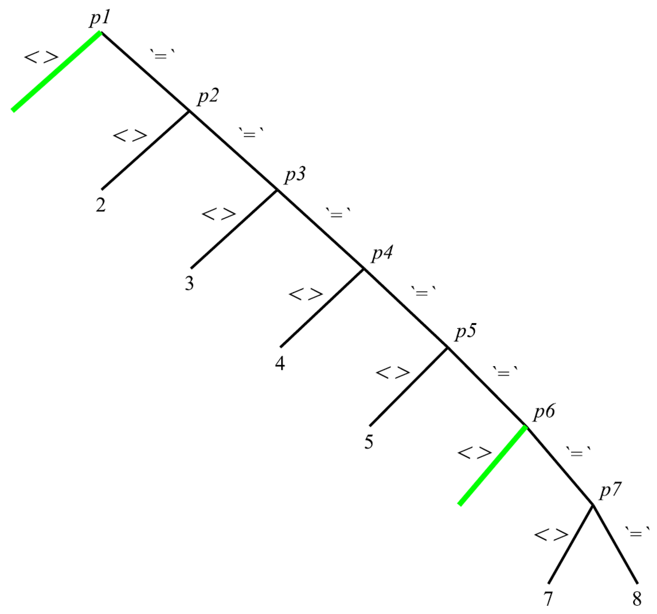
The full Maple code script following these steps and showing the full outcome of the relative computations can be found in Supplementary Materials. The resulting classification analysis for the Baker2013 model is shown in Figure 3.
Each solved determining equation is then used to determine the fluxes of conservation laws and the conservation laws (as per Definition 7 in Section 2.2) case-by-case. Table 2 summarises these results, which can be fully found as outputs to the GeM computational analysis in the Supplementary Materials.
As per the decision tree plot in Figure 3, the conservation law analysis of the Baker2013 model [16] identifies eight cases defined by the parametric conditions p 1 , p 2 , p 3 , p 4 , p 5 , p 6 and p 7 . Cases 1 and 6 differ in the conditions defining them but their conservation laws are equivalent. Both cases are solved via the “Direct” method, thus using the multiplier Λ 1 ( t , a ) = 0 to derive the two identical fluxes of conservation law Flux t = c 1 , where c 1 is an arbitrary constant. Using Definition 7—in particular div Φ [ u ] D x Φ [ u ] = 0 where Φ [ u ] = Φ ( x , u , u , , r u ) are known as the “fluxes of the conservation law”—the conservation law
c 1 D t = 0 D t = 0
can thus be written for the Baker2013 model by letting Φ [ u ] = Flux t = c 1 and simplifying the constant parameter c 1 out. The conservation law in Equation (21) describes a conservation of the time variable t within the pro- and anti-inflammatory cytokines’ dynamics. This conservation of time corresponds to conservation in energy [36,58], a well-known property of many physical and biological systems. In practical terms, conservation of energy implies that if a set of experimental assays was to be performed on the current model, their results would be reproduced in time. More formally, conservation of energy implies robustness of the predicted cytokines’ dynamics to time perturbations.
All other cases (namely, 2, 3, 4, 5, 7 and 8) yield the multiplier Λ 1 * ( t , a ) = c 1 + c 2 exp ( t ) , where c 1 and c 2 are two arbitrary constants. Due to the level of complexity of the Baker2013 model and the presence of the non-trivial multiplier Λ 1 * ( t , a ) in the unsolved flux expression, the “Direct” method cannot solve these other fluxes of conservation law. Both integration solver methods (i.e., homotopy 1 and homotopy 2) are also not compatible with these derivations, as they do not support the augmentation of arbitrary functions in the model, as discussed in Section 3.1. Thus, the scaling method is implemented by assuming a temporal symmetry generator X 1 = t from Equation (21), recovering Flux t = 0 . Consequently, no additional conservation law is found for the Baker2013 model.
In summary, the Baker2013 model predicts conservation of energy—i.e., experimental reproducibility—in some precisely defined parametric conditions of its parameter space. For the Baker2013 model to realistically reflect the evidence on RA, the results emerging from its robustness analyses must agree with its clinically observed disease phenotypes. In other words, the conservation of energy trends in the Baker2013 model must be consistent with the expected RA disease behaviours. As part of the complex RA disease phenotypic repertoire [20,47,52,59,60], inflammation flares are often clinically observed in patients [20,59,60]. Because of their oscillatory behaviour, clinical assays performed on a RA patient experiencing inflammation flares will not produce the same result consistently in time. In other words, experimental reproducibility is incompatible with inflammation flares. The Lie symmetry analysis on the Baker2013 model allows for some areas of its parameter space to not be bounded to conservation of energy (see Table 2 and Figure 3). This conditional existence of conservation of energy allows for the robust emergence of oscillatory phenotypes in the Baker2013 model, indicating that Lie symmetry allows identifying inflammation flares as an indicator of biological feasibility in RA modelling. To summarise, a comparison of the results of Lie symmetry-based conservation law analysis with the clinical RA evidence on inflammation flares allows performing a successful model evaluation check on the disease phenotypes predicted by the Baker2013 model.

4. Discussion

The aim of this paper is to explore novel analysis methods for the study of robustness in physiological modelling, and therefore to derive mathematically informed conclusions on a system’s response to perturbations. These conclusions are instrumental to propose testable predictions on the biological system under investigation. Robustness plays a key role in maintaining and adapting a system’s functionalities as a response to one or more changes in its environment [1,2,3]. Indeed, robustness holds interest in Systems Medicine, as its study allows investigating (i) how a patient’s state transitions from health to disease (and vice versa) under various stimuli, and (ii) how these changes are maintained in time [8,86,87,88]. In the context of drug-dependent remission of a disease, and its development after drug withdrawal in patients, robustness analyses enable investigating the differences between patients maintaining remission, thus achieving a robust remission state, and patients falling into relapse. Therefore, robustness analyses can assist in the identification of the mechanisms occurring in patients with drug-free remission that achieve a sustained health state, thus hypothesising how such a state may be induced.
Focussing on the ultimate aim of exploring analytical properties leading to sustained remission dynamics, this paper investigates robustness in the rheumatoid arthritis (RA) physiological system as a case study. In particular, robustness is investigated with respect to the model of pro- and anti-inflammatory cytokines in the RA-inflamed synovium published by Baker and colleagues [16]. A Lie symmetry analysis of the model is performed by investigating the conditions for the emergence of different conservation laws in the RA-inflamed synovium. Ultimately, the results are used to gain a deeper understanding of the properties characterising the system’s robustness. The Lie symmetry analytical approach identifies at most two different conservation law cases that the RA model can exhibit, alongside their parametric conditions for validity. In particular, a conservation law solely with respect to the time variable—known in the literature as “conservation of energy” and linked to experimental reproducibility [36,58]—is found for two out of the total set of eight emerging parametric combinations. This conservation law trend is then compared to the RA disease phenotypes observed clinically and experimentally [42,59,60,61] to conclude that the parameter-dependent existence of conservation of energy supports the emergence of inflammation flares in RA progression. Therefore, the Lie symmetry analysis indicates that the emergency of inflammation flares is of interest in the study of robustness, and therefore sustained RA remission or relapse, according to the conditional emergence of conservation of energy.
In other words, specific numerical parameter sets in the Baker model enable the robust emergence of experimental reproducibility in their predicted health or disease state. From a clinical point of view, each patient experiencing RA is characterised by a specific, personal set of numerical parameters that can be potentially derived from clinical testing. These numerical values can then be input into the analytical form of the conservation of energy conditions of existence derived in this paper to “personalise” the resulting insights ad hoc for a specific patient. Therefore, it will be potentially possible to identify which conservation law case is associated to the patient’s specific RA condition. In terms of remission and relapse, a patient in a state of achieved remission whose profile falls under conservation of energy validity is predicted to satisfy experimental reproducibility. Therefore, the acquired state of remission will be maintained robustly in time, i.e., any future assay performed on their RA condition will yield the same set of results. Similarly, a patient that falls into relapse and whose profile falls under conservation of energy validity is predicted to be in a robust state of relapse. On the other hand, patients whose profile is not compatible with conservation of energy validity will not be subject to experimental reproducibility, thus being in either a non-robust, evolving state of disease or a robust flaring conditions.
Considerations based on the experimental reproducibility of the findings were also used to perform model evaluation, concluding that the Baker2013 model can be used to describe the cytokine dynamics in the RA-inflamed synovium without loss of information, not only in terms of predicted temporal dynamics—as published by Baker and colleagues [16]—but also in terms of its structural robustness via its conservation laws.

4.1. Lie Symmetry Robustness Analysis Towards Sustained Drug-Free Remission in RA

The investigations performed in this paper show that a Lie symmetry-based approach can be effectively implemented to analytically derive the conservation laws of a physiological system. In particular, conservation law determination allows for the identification of the invariant parameters and variable identities within the studied system [2,29,73]. In a clinical context, the conservation laws arising from the mathematical structure of a physiological model can then be translated into the mechanisms allowing a robust characteristic of the disease to be achieved. For instance, conservation laws in a clinical context can be used to gain insights on the robust characteristics pushing a disease system towards (i) drug-dependent remission, (ii) drug-free remission maintained in time, and (iii) relapse.
In this paper, a robustness study through Lie symmetry-derived conservation laws is performed on the model of pro- and anti-inflammatory cytokines in the RA-inflamed synovium by Baker and colleagues [16] (i.e., the Baker2013 model). RA holds interest for Systems Medicine as the mechanisms governing the achievement and maintenance of both drug-dependent and drug-free remission are currently unknown [7,21,39,40]. In particular, treatment strategies that induce drug-dependent remission in (a minority of) RA patients do exist. However, this remission state is often lost upon drug withdrawal in favour of relapse [21,39,40]. To address this critical aspect, the robustness analyses proposed in this study enable a deeper analytical understanding of the RA mechanisms that may favour either robust remission or relapse in patients, thus offering a strategy towards the elucidation of RA remission mechanisms. The parameter-dependent conservation law with respect to time yielded by the Baker2013 model upon robustness analyses through Lie symmetry, often referred to as “conservation of energy” [36], reflects the conditional time-invariant property of pro- and anti-inflammatory cytokines’ dynamics in the RA-inflamed synovium. As briefly discussed in Section 3.2, conservation of energy is a well-known property of many biological systems, and it reflects the system supporting experimental reproducibility within its parameter space [36,58]. Clinically, experimental reproducibility reflects a patient’s state being robustly maintained in time in the absence of perturbations, as performing the same experimental assay at different time points, on the same patient, should not change its outcome. Consequently, conservation of energy being supported by the RA model reflects an unchanged system’s state in time that (i) is robust around its current state, and (ii) adapts to perturbations in favour of this same state. From a clinical point of view, a patient whose health or disease state is compatible with conservation of energy will be robust in time and will therefore indicate either maintained remission or severe relapse, respectively. On the other hand, a patient whose condition is not compatible with conservation of energy will not experience experimental reproducibility and will therefore be in a dynamical non-robust condition of disease—which is therefore appropriate for the application of treatment-like perturbations aiming to change this state towards remission.
In the present work, the Lie symmetry-based analysis on the RA model also shows that conservation of energy is not supported for all parametric conditions in the Baker2013 model (see Table 2 and Figure 3). Indeed, various parametrically defined conditional cases for conservation laws’ existence in the Baker2013 model do not yield any conserved quantities. This conditional “breakage” of the conservation of energy in the Baker2013 model does not support experimental reproducibility for all emerging disease phenotypes. From a clinical point of view, this conditional model characteristic can be reflected by the same patient’s disease state changing in time without the intervention of any kind of perturbation for some RA phenotypes. Indeed, from both clinical [20,47,52,59,60] and mathematical [16,41,89,90,91] points of view, RA is a complex disease, as it incorporates different disease stages and phenotypes which do not always align with experimental reproducibility. For instance, oscillatory inflammation behaviours can often be observed in RA patients. Clinically, these oscillations emerge as periodic flares of inflammation, followed by periods exhibiting a less severe inflammatory condition [16,20,41,59,60]. Sustained inflammation flares move a patient’s disease state through different degrees of disease severity repeatedly over time. Therefore, carrying out a clinical assay on a patient experiencing RA-induced inflammation flares will not yield the same results at different time points. The Lie symmetry-informed presence of parametric conditions in the Baker2013 model “breaking” conservation of energy indicates the presence of robust inflammation flares under a set of specific conditions. Therefore, a clinical interpretation of conservation of energy in the model allows for gaining insights on disease dynamics that may potentially lead to robust disease phenotypes, i.e., RA-specific inflammation flares.
The conditional presence of robust inflammation flares emerging from the proposed analysis provides a “map” towards the achievement of in silico drug-free remission in RA patients. The parameter and variable-based conditions for the emergence of the conservation of energy—as per Table 2, Figure 3 and the Supplementary Material—can be interpreted as analytical instructions for the existence of conservation of energy in the model parameter space. In future studies, these Lie symmetry investigation results could also be visualised through partitioning a system’s parameter space into areas reflecting how its conservation of energy conditions of existence change and meet.
Clinically derived data from a given patient could also potentially inform the quantitative identification of the unknown variables and parameters building the conditions of existence for conservation of energy. This further step would open room for the quantitative identification of treatment approaches built ad hoc for that individual patient. Once the parametric conditions for the existence of conservation of energy are found in terms of enumerated parameter and variable values and localised in a parameter space, it would be possible to hypothesise how to move between them—and therefore break the robust conditions around sustained disease states localised within them. The localised conservation of energy areas may then be used to inform both clinical decision-making and model evaluation. In other words, from a clinical point of view, each patient’s RA condition can be potentially defined by a set of numerical assay-derived parameters. Once input in the proposed analytical conditions of existence for conservation of energy, each patient’s state can be associated to a specific case depending on the numerically resolved parametric conditions. Thereafter, it will be potentially possible to personalise the hypothetical treatment-like perturbation that can be applied in silico towards the achievement of a robust state of remission.
To this purpose, further robustness analyses could be integrated into the proposed Lie symmetry methodology to provide additional information on sustained trends in a disease model, alongside their validity conditions. For instance, Linear Stability Analysis (LSA) is a mathematical methodology widely used to study a system’s behaviour around its equilibria [22]. In particular, LSA allows for the enumeration and quantitative identification of the stable health and disease states of a physiological model, as well as the dynamical trends around them [22]. For the Baker2013 RA model used in this paper as a case study, Baker and colleagues [16] perform a LSA to describe the dynamical characteristics of health and disease phenotypes under various mathematical conditions and perturbation hypotheses. Integrating such LSA insights into the conservation of energy results in Section 3.2 would open room for a further layer of information to be added to our current robustness investigations. For instance, it would enable the identification of the formalisms behind the emergence of different phenotypes driving—and possibly breaking—inflammation flares in the RA model parameter space. Or again, the equilibria information provided by LSA could be used to inform health and disease-specific conservation law behaviours in RA, therefore enabling more accurate and precise hypothesis-driven treatment towards sustained remission.
In summary, the Lie symmetry-based analysis performed in this paper paves the way to the quantitative investigation of (i) the existence and parametric extent of robust health- and disease-associated conservation laws, (ii) their distribution in a model’s parameter space, and (iii) the quantitative perturbations needed to move the system’s states between them. In the RA case study presented here, this approach would allow for the investigation of the conditions maintaining RA aggravation over time, thus yielding new information on RA progression in its most severe cases. This investigation would then allow a targeted exploration of the RA parameter space via treatment-like stimuli, potentially enabling practitioners to test the extent of a patient’s response to localised perturbations, e.g., reflecting a test therapy. Additional methodologies such as LSA could therefore be integrated to provide further information to the quantitative and parameter space-localised robustness insights gained via Lie symmetry analysis.

4.2. Lie Symmetry Analysis for Model Evaluation

From a more formally mathematical perspective, Lie symmetry analysis is argued to aid not only in robustness information, but also in model evaluation. From a mathematical angle, various formally different models can yield the same dynamics for one same disease condition. Model evaluation and selection are thus paramount to determine which candidate model is best able to describe both clinical and experimental evidence. However, this procedure can be challenging, as multiple models might fit evaluation and selection criteria equally well [24]. In this paper, it is argued that Lie symmetry-based conservation laws provide powerful insights into this issue. A clinical interpretation of the emerging conservation laws of a physiological model can provide rich information on the feasibility of disease phenotypes predicted by dynamical modelling, based on the underlying model structure. Indeed, the comparison of conservation laws and temporal dynamics onto the same parameter space can restrict the set of predicted disease behaviours, based on their feasible coexistence. Therefore, model evaluation and selection can be more accurately performed not only based on how well a putative model fits experimental and clinical data, but also on how well the underlying mathematical structure reflects biological feasibility.
The Baker2013 model case study gives an example of how conservation laws can aid in modelling evaluation. As we have discussed, RA is a complex disease and incorporates different disease stages and phenotypes, such as periodic flares of inflammation [16,20,41,59,60]. From a modelling selection and validation perspective, the best model sufficiently reproducing RA dynamics would admit such oscillatory behaviour. Baker and colleagues [16] show that flares in the form of limit cycles are qualitatively admitted by the Baker2013 model; thus, the published dynamical modelling provides information on the mathematical existence of flares in the RA-inflamed synovium. At the same time, the results of the conservation law analysis in Section 3.2 shows that conservation of energy is a characteristic of the Baker2013 model, and it has been argued that it is an indicator of experimental reproducibility—unlike inflammation flares. Therefore, it is foreseen that the Baker2013 model will not sufficiently reproduce RA dynamics if all its oscillatory phenotypes coexist in the same parameter space sections as conservation of energy. The conservation law analysis in Section 3.2 allows for a series of conditions where no conservation laws exist, thus breaking conservation of energy. In other words, there are conditions on the existence of the conservation of energy yielded by the Baker2013 model that allow for the reasonable existence of inflammation flares, as sustained flares could potentially lie in the parameter space areas not imposing experimental reproducibility.
In summary, the conservation of energy trends of the Baker2013 model—arising from our proposed Lie symmetry-based analysis—allow critically evaluating how well the model reflects the inflammation flare disease phenotype clinically expected [20,41,59,60]. Therefore, it is possible to conclude that the Baker2013 model can potentially reflect the oscillatory nature of RA-induced inflammation, given that its structure allows for the feasible coexistence of both experimental reproducibility—i.e., conservation of energy—and oscillatory phenotypes. In the future, a more accurate evaluation of the Baker2013 model building on these observations will involve the mapping of both oscillatory phenotypes and conservation of energy areas in its parameter space, to then visually compare how the two meet and coexist in the same phenotypic repertoire.

4.3. Modelling Perspectives

The proposed Lie symmetry methodology is not limited to Ordinary Differential Equations (ODEs) systems (such as the Baker2013 model in Equation (5)) to study their robustness characteristics and inform model evaluation. Indeed, it can be extended to all Differential Equation (DE) models of physiological systems. Lie symmetry analysis can be applied to DE models of various nature, such as higher-order and multiple-variables ODEs and Partial Differential Equations (PDEs). Indeed, while some limitations emerge with Lie symmetry analysis of first-order ODEs, the methodology can be applied to both higher-order ODE systems and PDEs. The implementation to more complex ODE and PDE physiological system is analytically equivalent, and the use of the computational tools aiding in conservation law derivation is largely unchanged [32,67,72,82]. Thus, the proposed methodology could potentially be applied to other physiological systems of different spatio-temporal scaling.
For instance, DE models of various granularity of autoimmune disorders other than RA [7] can be studied via Lie symmetry analysis. As an example, RA modelling could be investigated further to explore robust cell-led mechanisms involved in RA progression. One of the main assumptions that was made in the Baker2013 model is the simplification of all cellular behaviour variability. This assumption allows modelling the synovium as a spatially homogeneous collection of cells [16,41]. While easing the model’s definition and analysis, this assumption also prevents to gain a more in-depth understanding of the specific cell-led mechanisms involved in RA progression. Other RA models take into account the specific mechanisms involved in the disease, albeit by complicating the mathematical formalisms they use [41]. Jit and colleagues [92] used a four-variable first-order ODE model to investigate the molecular-level dynamics of Tumour Necrosis Factor- α (TNF- α ) in RA, including the formation of ligand–receptor and antigen–antibody complexes, as well as the binding process of TNF- α to cell surface receptors. Thereafter, they studied and predicted both the short- and long-term benefits of various treatment techniques inhibiting TNF- α . To do so, the authors first focused on the identification of the steady states of the RA model, distinguishing between health and pathological states in terms of TNF- α concentrations. Subsequently, they performed a parameter space exploration of the system, with the aim of reproducing various treatment conditions [41,92]. Odisharia and colleagues [90] developed a five-variable ODE model to describe interactions between B cells, T cells and cells forming in the cartilage once tocilizumab treatment is applied. The authors study this RA model by investigating the resulting dynamics numerically, including cartilage degradation, as various parameters are changed [41,90]. Using the proposed Lie symmetry-based methodology on such models, the robustness of these systems can potentially be investigated, alongside their model evaluation, thus deepening the current understanding of RA. A common set of conservation laws arising in RA models can then be potentially identified. Therefore, this common set of RA conservation laws could be used to find a common set of robust characteristics linking together different healthy and diseased steady states.
This information could be used to further define more realistic RA models. To better understand this, we can think about the case study investigated in this paper. A pre-constructed model of RA dynamics (i.e., the Baker2013 model [16]) is used to inform the conservation law analysis, explore robustness and derive model evaluation observations. However, Lie symmetry analysis results could also work in the opposite direction, i.e., informing a model with respect to the RA robustness gathered by comparing multiple models’ robustness results. This bidirectional approach could help not only in evaluating robustness and model formalisms but also in optimising the dynamics definitions embedded in the models.
Finally, data fitting may be potentially performed to estimate the model parameters and experimentally evaluate the results discussed in this paper. For a mathematical model to be biologically relevant, most—but optimally all—its parameters must be derived from clinical or experimental data. The complexity of the model will then heavily depend on the availability of the biological data used to support the parameter choices and to validate the resulting dynamics [41]. However, in RA, it is difficult to collect clinical and experimental data from in vivo and in vitro studies relevant to human research [41,93,94,95]. Indeed, RA dynamics in humans do not develop as in animals, and must therefore be induced therapeutically with a short disease lifetime in patient samples [41,94]. While such clinical trials and studies provide the optimal biologically relevant setting for RA data collection, the information that can be gathered from patients is limited [41,94]. Nonetheless, RA mathematical studies such as the ODE model by Jit and colleagues [92] use various experimental information to estimate their parameters [41]. Therefore, in spite of the currently limited availability of RA experimental data to validate the robustness analysis performed for the RA model of Baker and colleagues [16], there is room for a more accurate experimentally and clinically based parameter evaluation and investigation. Much research is currently being performed on the use and discovery of RA biomarkers data [96] and their correlation with cytokine profiles [97]. Cytokines themselves are being considered as RA biomarkers, as recent technological developments have allowed for large cytokinetic data sets to be generated from small patient body fluid volumes [98]. Therefore, in the future there will be potential room for the clinical data evaluation of the robustness observations performed for the RA case study in this paper. For instance, Nakada and colleagues [99] have recently investigated the interplay between various cytokines involved in RA progression via a data-informed quantitative ODE model to explain inter-patient variability in anti-inflammatory treatments [41]. Although this model is pharmacokinetic [99], and therefore mostly focuses on the time course of time exposure [41], the methodologies used to manipulate the experimental and clinical data could potentially be applied in the future to validate the robustness observations from this case study.
The applicative scope of this Lie symmetry robustness analysis is wider than the RA test case, and can cover other dynamical DE models of health and disease. For instance, the Lie symmetry analytical methodology can be used to unveil mechanisms of disease in cancer. Cell cycle modelling optimally fits this aim, as its dysregulation is strongly linked to oncogenesis [4,7,13,100]. Given the evolutionary conservation of the cell cycle network across eukaryotes, minimal cell cycle networks can be used to investigate key dysregulated components often mutated in disease [4]. The cell cycle can be modelled as a network of cyclin-dependent kinases, which can then be investigated in terms of its robustness properties [4,13]. The arising Lie symmetry-based conservation laws’ trends can then be interpreted in terms of the phenotypic behaviours observed in the clinical and experimental literature, therefore opening room to discussion about key robust dysregulation mechanisms in aberrant cell growth and division. For example, minimal autonomous cell cycle oscillator designs [4,101] can be used as case studies for future Lie symmetry robustness investigations. Studying shifts in these minimal models’ phenotypic regimes with respect to their ability to exhibit oscillations can then be further investigated by identifying their underlying conservation laws. This information would then give further insights into what network components and interactions remain conserved under set parametric conditions, and therefore what robust characteristics remain unchanged under phenotypic shifts in cell cycle dysregulation.

4.4. Limitations and Advances

The proposed and discussed Lie symmetry-based conservation law analysis for robustness investigations of physiological models holds room for analytical, computational and technical growth.
From an analytical perspective, the proposed Lie symmetry methodologies can be applied to find the discrete Lie point symmetries—and therefore the associated concentration laws—of all given ODEs of order higher than one and PDEs [32,37,84]. In this case, the system of ODEs or PDEs would not need any analytical preparation to account for any Lie symmetry analysis assumption, and could straightforwardly be input in a computational solver of choice (here the GeM Maple software package). However, as discussed in Section 3.1, the Lie symmetry analyses cannot be applied directly to a system of first-order ODEs. Indeed, according to the relevant literature on Lie algebra, all first-order ODEs and their systems admit an infinite-dimensional Lie algebra of infinitesimal operators—and therefore an infinite-dimensional set of conservation laws [32,37,84]. This analytical bottleneck implies that all attempts to find an exhaustive set of conservation laws for first-order ODEs would be insufficient, complex and computationally expensive. Therefore, an analytical limitation of first-order ODE systems is that these need to be algebraically manipulated and recast into an equivalent higher-order form before being computationally analysed for their conservation laws. The Baker RA model analysed in this paper as a case study represents such an example. However, as shown in Section 3.1, the analytical manipulations needed to prepare its form to Lie symmetry analyses can be performed with no issues either analytically (as done here) or computationally.
The proposed Lie symmetry-based conservation law analysis holds room for growth also from a computational perspective. First, the limitations of the computational techniques used in the Lie symmetry and conservation law analysis of the RA-inflamed synovium case study is discussed. As per Section 2.3, the Lie symmetry-based conservation law analysis has been carried out using the Maple GeM symbolic software package for general symmetry and conservation law analysis [72,73,78,79]. As previously argued, the Baker2013 model (Equation (5) [16]) cannot be directly input into the GeM package. Indeed, this model is a first-order system of ODEs of the form shown in Equation (16), and, as such, admits an infinite-dimensional Lie algebra of infinitesimal operators [32,37,84]. Therefore, a recasting is performed with respect to the two-variables first-order system of ODEs in Baker2013 to a single equivalent one-variable second-order ODE, namely Equation (18). Moreover, its form had to be further manipulated to adapt to the GeM package limitations in handling non-transcendental functions, [74,78,82] here powers. This limitation is brought by the rifsimp symbolic routine [85] used in the GeM package [74,78,82]. To do so, a series of arbitrary functions (i.e., Equation (19)) were introduced, which allowed rewriting the Baker2013 model in the GeM-friendly form in Equation (20). These change-of-order and non-transcendental functions manipulations are algebraic and must be performed analytically. In future studies, there will be room for the computational implementation of these two manipulations via Maple-based routines. This would ultimately allow a user to straightforwardly input their DE model in the GeM routine without necessarily having to cope with potentially complex analytical manipulations.
Furthermore, the potential of the GeM package for the computation of fluxes of conservation laws is limited by introducing arbitrary functions to handle non-transcendental functions in the model of interest. As per Section 2.3, the GeM package offers four different methods to compute the fluxes of conservation laws of a system of DEs, which are briefly described in Table 1. For the conservation law analysis in Section 3.2, two of these methods are employed: the “direct” and the “scaling” methods, which are the only two available flux computation methods allowing the use of arbitrary functions within the GeM package. Indeed, the two integration-based methods, “homotopy 1” and “homotopy 2”, do not support the integration of arbitrary functions. Therefore, the potential of the GeM package for the computation of fluxes of conservation laws is limited by introducing arbitrary functions to handle non-transcendental functions in the model of interest. By extension, it can be said that the rifsimp symbolic routine [85] implemented for simplification purposes in the GeM package limits the analytical potential of GeM for the computation of fluxes of conservation laws, due to non-transcendental functions’ intolerance. A future computational expansion could, therefore, include the implementation of an alternative Maple routine for the simplification of overdetermined DE systems within the GeM routine. One such package, for instance, is the Janet Maple routine, enabling the simplification of linear PDE systems [102], not unlike rifsimp.
Alternatively, other computational techniques and routines other than GeM are available to perform Lie symmetry analysis on DE systems. One such computational routine ad hoc for first-order ODE systems is the “symSys_1st_ODEs” Python and LaTeX-based project, developed by Borgqvist and colleagues [26]. As discussed in Section 3.1, all first-order ODE systems admit an infinite-dimensional Lie algebra of infinitesimal operators [32,37,84]. From a practical point of view, computing the infinitesimal generators of Lie symmetries for a system of first-order ODEs without recasting the system to a higher order will imply resorting to some kind of guess on the form of the generator being searched, which will be referred to as an “Ansatz” [26,84]. Indeed, symSys_1st_ODEs uses such Ansätze to compute the infinitesimal generators of symmetry (as Definition 4) of first-order ODE systems [26]. These Ansätze will consequently restrict the range of search to those generators that mostly agree with the form being guessed. Indeed, while symSys_1st_ODEs proves to be successful in deriving a set of infinitesimal generators of symmetry for various first-order ODE systems, such as the Susceptible–Infected–Recovered (SIR) model, its derivations are limited to polynomial Ansätze. Consequently, its search for generators of symmetry will exclude non-transcendental functions such as trigonometric functions. As far as we are aware, there is currently no analytical methodology that allows computing the complete set of all the symmetries of first-order ODEs that does not involve the input of some Ansatz. Moreover, the implementation of this project is limited by the symbolic calculations performed using the SymPy Python library [103], which can potentially lead to very long and expensive computational runs. Therefore, in this paper, the Maple GeM software package has been used for the Lie symmetry-based robustness analysis instead of symSys_1st_ODEs. Nonetheless, an in-depth comparison of the symSys_1st_ODEs and GeM packages could potentially allow integrating their individual strengths in a refined computational pipeline.
An analytical consideration on Lie symmetries may also be drawn from the work presented in this paper. All the Lie symmetry-based robustness investigations are focused on local conservation laws. As seen in Definition 7 (Section 2.2), all the derived conservation laws for the models considered in this paper depend only on the independent and the dependent variables of the system [104], and are thus local. However, conservation laws could also be written not only in terms of the system’s variables but also their derivatives and differentials [104]. Such so-called nonlocal conservation laws stem from potential systems which can be derived from the original model using its local conservation laws [74,104]. Nonlocal conservation laws usually arise in systems involving arbitrary functions and constant parameters [74], much like the Baker2013 model (Equation (5) [16]). Studying the nonlocal Lie symmetries and conservation laws of a physiological system would widen the potential of the proposed Lie symmetry-based conservation law analysis, as it would not only expand robustness studies and model evaluations but it would also allow obtaining solutions of the DE systems [104]. The GeM package includes the computational tools needed to perform such nonlocal analyses [72,73,78,79], and it would thus aid in expanding future studies in this direction.

5. Conclusions

This paper proposes the use of a Lie symmetry-based methodology towards robustness investigations and model evaluation in physiological systems. For many complex diseases, such as rheumatoid arthritis (RA), it is currently possible to clinically achieve drug-free remission for numerous patients. However, the tools to identify the mechanisms yielding drug-free remission are currently lacking [21]. Building and investigating dynamical models of disease systems, with a focus on uncovering their robustness mechanisms, may help in this task, although it requires the use of ad hoc analytical and mathematical formulations [26,32,67].
Here, Lie symmetry-based conservation law analysis is proposed as a mathematical tool to undercover the robustness characteristics of a disease model, to then inform in silico sustained drug-free remission of the disease. When investigating the development of a patient’s state from health to disease, and possibly to learn how to bring the system from disease back to health, it is key to know how the system responds to stimuli in order to understand how these disease states change with time and upon perturbation. Therefore, informed decisions based on what it is known about the physiological system’s robustness will have to be made to hypothesise how to induce a different state and to maintain that change in time—for instance, from a disease state to a drug-free remittance state. The proposed Lie symmetry-based methodology allows gaining such a robustness understanding from in silico studies of a physiological system’s model. In particular, this approach can be used to derive model-specific conservation laws, providing information on what characteristics of a system remain unchanged under various stimuli, as well as the specific conditions to be satisfied for their maintenance. Therefore, from a clinical standpoint, it would be possible to predict how the system’s structure sustains and possibly adapts to hypothetical treatment-like perturbations.
Ultimately, this Lie symmetry study can contribute to paving the way towards one of the main aims of Systems Medicine, i.e., personalised treatment of disease conditions. For example, for a patient currently undergoing medical screening towards a disease’s diagnosis, the Lie symmetry robustness analysis proposed will allow using this patient’s medical record to: (i) clinically interpret the conservation laws arising for their specific condition, (ii) enumerate their validity criteria ad hoc for the patient under study, and (iii) hypothesise how to either maintain or break one or more conservation laws towards the achievement of sustained remission. Moreover, this methodology could be applied not only to clinical practice but also to the more mathematically based side of Systems Medicine. Indeed, the resulting analysis can be used to inform currently existing disease models, to ultimately refine their predictive in silico potential. Successively, the newly refined physiological models can be practically used to inform more precise and accurate personalised treatment hypotheses.

Supplementary Materials

The following supporting information can be downloaded at: https://www.mdpi.com/article/10.3390/sym18071143/s1, Baker2013 Maple script: “Baker2013_GeM_ locconslaws_arbfun.mw” and “Baker2013_Maple_script.pdf”. The following colour legend is used in the Supplementary Material Scripts: green for notes and comments, brown for code input, and blue for code output.

Author Contributions

Conceptualisation, M.B.; methodology, M.B.; software: A.D.C.; validation, A.D.C.; formal analysis, A.D.C.; investigation, A.D.C. and M.B.; writing—review and editing, A.D.C. and M.B.; visualisation, A.D.C. and M.B.; supervision, M.B.; project administration, M.B.; funding acquisition, M.B. All authors have read and agreed to the published version of the manuscript.

Funding

This research was funded by the Systems Biology Grant of the University of Surrey to M.B. A.D.C. was funded by a studentship in Systems Biology and Medicine of the Faculty of Health and Medical Sciences (FHMS) of the University of Surrey to M.B.

Data Availability Statement

Data supporting the reported results generated and analysed in this study can be found in the main text and Supplementary Materials.

Acknowledgments

The authors thank Maria Clara Nucci for suggesting the Maple software to retrieve Lie symmetries and further reading material on their reduction, Alexey Shevyakov for sharing the GeM software package, and Irene Zorzan for checking the mathematical derivation of the linear stability analysis.

Conflicts of Interest

The authors declare no conflicts of interest.

Abbreviations

The following abbreviations are used in this manuscript:
SLESystemic Lupus Erythematosus
DEDifferential Equation
ODEOrdinary Differential Equation
SIRSusceptible–Infected–Recovered
RARheumatoid Arthritis
IL-1Interleukin-1
TNF- α Tumour Necrosis Factor- α
IL-1RaInterleukin-1 Receptor Antagonist
IL-10Interleukin-10
IL-1RIL-1 Receptor
COVID-19Coronavirus Disease 2019
PDEPartial Differential Equation
LSALinear Stability Analysis

Appendix A. Change-of-Order Manipulation

As discussed more in depth in Section 3.1, the first step in the conservation law analysis of the Baker2013 model (Equation (5) [16]) is to rearrange its form so that it is optimal for Lie symmetry investigations. In particular, two manipulations are performed: a change-of-order manipulation and a transcendental functions manipulation. Due to the complexity of the steps in the change-of-order manipulation, the full algebra is shown in this appendix.
A change-of-order manipulation allows one to recast a system of first-order Ordinary Differential Equations (ODEs) into one or more higher-order ODEs. Indeed, according to the scientific literature on Lie symmetries, all systems of first-order ODEs admit an infinite-dimensional Lie algebra of infinitesimal operators as per Definition 4 [32,37,84]. Therefore, performing Lie symmetry analysis for a system of first-order ODEs is potentially expensive and non-exhaustive [32,37]. As a result, the first-order system of ODEs analysed in this paper—i.e., the Baker2013 model [16]—is recast into the second-order ODE in Equation (18).
This change-of-order manipulation can be summarised in four steps, as discussed in Section 3.1:
  • Consider the two-variable first-order ODE model to be of the form
    p ( t ) = F t , p ( t ) , a ( t ) = 0 ( i ) a ( t ) = G t , p ( t ) , a ( t ) = 0 ( i i ) .
  • Using ( i i ) , find an expression for p in terms of a and a only, which will be labelled ( i i i ) for ease.
  • Differentiate ( i i i ) with respect to time t in order to derive an expression for p , which will be labelled ( i v ) for ease.
  • Input ( i i i ) and ( i v ) into ( i ) and manipulate the equation in order to derive an expression for a ( t ) —4 d 2 a ( t ) d t 2 .
Thus, the new expression for the original first-order ODE model will be a second-order ODE in terms of a ( t ) , a ( t ) and a ( t ) only, without any loss of information.
The full steps below show how to recast the first-order system of ODEs in the Baker2013 model (Equation (5) [16]) into an equivalent second-order ODE (Equation (18)).
  • Consider the Baker2013 model
    d p d t = γ p + 1 1 + a 2 α 1 + α 2 p 2 1 + p 2 ( i ) d a d t = a + α 4 p 2 α 3 2 + p 2 ( i i )
    in Equation (5), where its dimensionless parameters are interpreted as discussed in Section 2.1 [16]:
    (a)
    α 1 = c 0 = c 0 c 3 c 2 d a is the basal pro-inflammatory cytokines’ production rate;
    (b)
    α 2 = c 1 = c 1 c 3 c 2 d a is the additional pro-inflammatory cytokines’ production rate thanks to their self-upregulation;
    (c)
    α 3 = c 6 d a c 3 = c 6 c 2 is the pro-inflammatory cytokines’ concentration for half-maximal anti-inflammatory cytokines’ production;
    (d)
    α 4 = c 5 c 4 d a is the anti-inflammatory cytokines’ production rate;
    (e)
    γ = d p d a is the ratio between the pro-inflammatory cytokines’ degradation rate d p and the anti-inflammatory cytokines’ d a .
  • Use the ODE ( i i ) and algebraically manipulate it as
    ( i i ) a = a + α 4 p 2 α 3 2 + p 2 expand the denominator a = a α 3 2 a p 2 + α 4 p 2 α 3 2 + p 2 multiply the denominator out a α 3 2 + p 2 = a α 3 2 a p 2 + α 4 p 2 expand the terms a α 3 2 + a p 2 = a α 3 2 a p 2 + α 4 p 2 bring all p 2 terms on the left - hand side a p 2 + a p 2 α 4 p 2 = a α 3 2 a α 3 2 collect p 2 p 2 a + a α 4 = a α 3 2 a α 3 2 rearrange for p 2 p 2 = α 3 2 a + a a + a α 4 find the positive and negative roots p ± = ± α 3 a + a a + a α 4 .
    To get biologically reasonable solutions, we want p ± to be real and greater than or equal to zero. Therefore, we restrict the range of values for a to a a , a + α 4 by setting a + a a + a α 4 0 . Then, we can write the biologically reasonable expression for p in terms of a and a only, given a a , a + α 4 , as:
    p = α 3 a + a a + a α 4 . ( i i i )
  • Differentiate ( i i i ) with respect to t as
    p = d d t α 3 a + a a + a α 4 perform the differentiation = α 3 2 a + a a + a α 4 1 / 2 ( a + a ) ( a + a α 4 ) ( a + a ) ( a + a ) ( a + a α 4 ) 2 expand the terms = α 3 2 a + a a + a α 4 1 / 2 a 2 + a a α 4 a + a a + a a α 4 a a a a a a a a 2 ( a + a α 4 ) 2 simplify = α 3 α 4 2 a + a a + a α 4 1 / 2 a + a ( a + a α 4 ) 2 use a common power = α 3 α 4 2 a + a α 4 a + a · ( a + a ) 2 ( a + a α 4 ) 4 3 1 / 2 multiply through = α 3 α 4 2 ( a + a ) 2 ( a + a ) ( a + a α 4 ) 3 1 / 2 rewrite = α 3 α 4 2 ( a + a ) 2 ( a + a ) ( a + a α 4 ) 3 , ( i v )
    in order to derive the expression for p , once again given a a , a + α 4 for the existence of biologically reasonable solutions.
  • Input ( i i i ) and ( i v ) into ( i ) and rearrange such that it is possible to derive
    α 3 α 4 2 ( a + a ) 2 ( a + a ) ( a + a α 4 ) 3 = γ α 3 a + a a + a α 4 + 1 1 + a 2 α 1 α 2 α 3 2 a + a a + a α 4 1 α 3 2 a + a a + a α 4 1 i . expand the denominator in the second term of the square bracket : α 3 α 4 2 ( a + a ) 2 ( a + a ) ( a + a α 4 ) 3 = γ α 3 a + a a + a α 4 + + 1 1 + a 2 α 1 α 2 α 3 2 a + a a + a α 4 a + a α 4 α 3 2 a α 3 2 a a + a α 4 1 ii . multiply the two expanded terms in the square bracket : α 3 α 4 2 ( a + a ) 2 ( a + a ) ( a + a α 4 ) 3 = γ α 3 a + a a + a α 4 + + 1 1 + a 2 α 1 α 2 α 3 2 a + a a + a α 4 a + a α 4 a + a α 4 α 3 2 a α 3 2 a iii . simplify the resulting term : α 3 α 4 2 ( a + a ) 2 ( a + a ) ( a + a α 4 ) 3 = γ α 3 a + a a + a α 4 + 1 1 + a 2 α 1 α 2 α 3 2 a + a a + a α 4 α 3 2 a α 3 2 a iv . inside the square bracket , collect the common factors in the denominator : α 3 α 4 2 ( a + a ) 2 ( a + a ) ( a + a α 4 ) 3 = γ α 3 a + a a + a α 4 + 1 1 + a 2 α 1 α 2 α 3 2 a + a a ( 1 α 3 2 ) + a ( 1 α 3 2 ) α 4
    v . multiply out the α 3 α 4 2 term on the left - hand side of the equation : ( a + a ) 2 ( a + a ) ( a + a α 4 ) 3 = 2 γ α 4 a + a a + a α 4 + 2 α 3 α 4 ( 1 + a 2 ) α 1 α 2 α 3 2 a + a a ( 1 α 3 2 ) + a ( 1 α 3 2 ) α 4 vi . resolve the square root by elevating both sides to the power of two : ( a + a ) 2 ( a + a ) ( a + a α 4 ) 3 = 2 γ α 4 a + a a + a α 4 + 2 α 3 α 4 ( 1 + a 2 ) α 1 α 2 α 3 2 a + a a ( 1 α 3 2 ) + a ( 1 α 3 2 ) α 4 2 vii . multiply over the denominator on the left - hand side of the equation : ( a + a ) 2 = ( a + a ) ( a + a α 4 ) 3 2 γ α 4 a + a a + a α 4 + 2 α 3 α 4 ( 1 + a 2 ) α 1 α 2 α 3 2 a + a a ( 1 α 3 2 ) + a ( 1 α 3 2 ) α 4 2 viii . resolve the squared term on the left - hand side by applying a square root to both sides of the equation : a + a = a a ( a + a α 4 ) 3 / 2 2 γ α 4 a + a a + a α 4 + 2 α 3 α 4 ( 1 + a 2 ) α 1 α 2 α 3 2 a + a a ( 1 α 3 2 ) + a ( 1 α 3 2 ) α 4 ix . rearrange the above expression to derive the second - order one - variable ODE : a = a + 2 α 4 a a ( a + a α 4 ) 3 / 2 1 α 3 ( 1 + a 2 ) α 1 α 2 α 3 2 a + a a ( 1 α 3 ) + a ( 1 α 3 ) α 4 γ a + a a + a α 4 given a a , a + α 4 for the existence of biologically reasonable solutions , once again .

References

  1. Masel, J.; Siegal, M.L. Robustness: Mechanisms and consequences. Trends Genet. 2009, 25, 395–403. [Google Scholar] [CrossRef] [PubMed]
  2. Lesne, A. Robustness: Confronting lessons from physics and biology. Biol. Rev. Camb. Philos. Soc. 2008, 83, 509–532. [Google Scholar] [CrossRef] [PubMed]
  3. Kitano, H. Biological robustness. Nat. Rev. Genet. 2004, 5, 826–837. [Google Scholar] [CrossRef] [PubMed]
  4. Mondeel, T.D.G.A.; Ivanov, O.; Westerhoff, H.V.; Liebermeister, W.; Barberis, M. Clb3-centered regulations are recurrent across distinct parameter regions in minimal autonomous cell cycle oscillator designs. npj Syst. Biol. Appl. 2020, 6, 8. [Google Scholar] [CrossRef] [PubMed]
  5. Kaizu, K.; Ghosh, S.; Matsuoka, Y.; Moriya, H.; Shimizu-Yoshida, Y.; Kitano, H. A comprehensive molecular interaction map of the budding yeast cell cycle. Mol. Syst. Biol. 2010, 6, 415. [Google Scholar] [CrossRef] [PubMed]
  6. Casey, M.J.; Stumpf, P.S.; MacArthur, B.D. Theory of cell fate. Wiley Interdiscip. Rev. Syst. Biol. Med. 2020, 12, e1471. [Google Scholar] [CrossRef] [PubMed]
  7. Ugolkov, Y.; Nikitich, A.; Leon, C.; Helmlinger, G.; Peskov, K.; Sokolov, V.; Volkova, A. Mathematical modeling in autoimmune diseases: From theory to clinical application. Front. Immunol. 2024, 15, 1371620. [Google Scholar] [CrossRef] [PubMed]
  8. Ma, C.; Gurkan-Cavusoglu, E. A comprehensive review of computational cell cycle models in guiding cancer treatment strategies. npj Syst. Biol. Appl. 2024, 10, 71. [Google Scholar] [CrossRef] [PubMed]
  9. Coelho, P.M.B.M.; Salvador, A.; Savageau, M.A. Quantifying global tolerance of biochemical systems: Design implications for moiety-transfer cycles. PLoS Comput. Biol. 2009, 5, e1000319. [Google Scholar] [CrossRef] [PubMed]
  10. Schultz, A.; Mehta, S.; Hu, C.W.; Hoff, F.W.; Horton, T.M.; Kornblau, S.M.; Qutub, A.A. Identifying Cancer Specific Metabolic Signatures Using Constraint-Based Models. Pac. Symp. Biocomput. 2017, 22, 485–496. [Google Scholar] [CrossRef] [PubMed]
  11. Brady, R.; Enderling, H. Mathematical Models of Cancer: When to Predict Novel Therapies, and When Not to. Bull. Math. Biol. 2019, 81, 3722–3731. [Google Scholar] [CrossRef] [PubMed]
  12. Perche, F.; Torchilin, V.P. Cancer cell spheroids as a model to evaluate chemotherapy protocols. Cancer Biol. Ther. 2012, 13, 1205–1213. [Google Scholar] [CrossRef] [PubMed]
  13. Hamis, S.J.; Kapelyukh, Y.; McLaren, A.; Henderson, C.J.; Wolf, C.R.; Chaplain, M.A.J. Quantifying ERK activity in response to inhibition of the BRAF600E-MEK-ERK cascade using mathematical modelling. Br. J. Cancer 2021, 125, 1552–1560. [Google Scholar] [CrossRef] [PubMed]
  14. Yazdani, A.; Bahrami, F.; Pourgholaminejad, A.; Moghadasali, R. A biological and a mathematical model of SLE treated by mesenchymal stem cells covering all the stages of the disease. Theory Biosci. 2023, 142, 167–179. [Google Scholar] [CrossRef] [PubMed]
  15. Fernández Massó, J.R. Systems Medicine of Autoimmune Diseases: From Understanding Complexity to Precision Treatments. In Immune Rebalancing; Boraschi, D., Penton-Rol, G., Eds.; Academic Press: Cambridge, MA, USA, 2016; Chapter 9; pp. 173–189. [Google Scholar] [CrossRef]
  16. Baker, M.; Denman-Johnson, S.; Brook, B.S.; Gaywood, I.; Owen, M.R. Mathematical modelling of cytokine-mediated inflammation in rheumatoid arthritis. Math. Med. Biol. 2013, 30, 311–337. [Google Scholar] [CrossRef] [PubMed]
  17. Kaur, G.; Ahmad, N. On Study of Immune Response to Tumor Cells in Prey-Predator System. Int. Sch. Res. Not. 2014, 2014, 346597. [Google Scholar] [CrossRef] [PubMed]
  18. Kareva, I.; Luddy, K.A.; O’Farrelly, C.; Gatenby, R.A.; Brown, J.S. Predator-Prey in Tumor-Immune Interactions: A Wrong Model or Just an Incomplete One? Front. Immunol. 2021, 12, 668221. [Google Scholar] [CrossRef] [PubMed]
  19. Gonzalez, H.; Hagerling, C.; Werb, Z. Roles of the immune system in cancer: From tumor initiation to metastatic progression. Genes Dev. 2018, 32, 1267–1284. [Google Scholar] [CrossRef] [PubMed]
  20. Jahid, M.; Khan, K.U.; Rehan-Ul-Haq; Ahmed, R.S. Overview of Rheumatoid Arthritis and Scientific Understanding of the Disease. Mediterr. J. Rheumatol. 2023, 34, 284–291. [Google Scholar] [CrossRef] [PubMed]
  21. Coyle, C.; Ma, M.; Abraham, Y.; Mahony, C.B.; Steel, K.; Simpson, C.; Guerra, N.; Croft, A.P.; Rapecki, S.; Cope, A.; et al. NK cell subsets define sustained remission in rheumatoid arthritis. JCI Insight 2024, 9, e182390. [Google Scholar] [CrossRef] [PubMed]
  22. Neri, I.; Metz, F.L. Linear stability analysis of large dynamical systems on random directed graphs. Phys. Rev. Res. 2020, 2, 033313. [Google Scholar] [CrossRef]
  23. Bicker, J.; Alves, G.; Falcão, A.; Fortuna, A. Timing in drug absorption and disposition: The past, present, and future of chronopharmacokinetics. Br. J. Pharmacol. 2020, 177, 2215–2239. [Google Scholar] [CrossRef] [PubMed]
  24. Ohlsson, F.; Borgqvist, J.; Cvijovic, M. Symmetry structures in dynamic models of biochemical systems. J. R. Soc. Interface 2020, 17, 20200204. [Google Scholar] [CrossRef] [PubMed]
  25. Morohashi, M.; Winn, A.E.; Borisuk, M.T.; Bolouri, H.; Doyle, J.; Kitano, H. Robustness as a measure of plausibility in models of biochemical networks. J. Theor. Biol. 2002, 216, 19–30. [Google Scholar] [CrossRef] [PubMed]
  26. Borgqvist, J.; Ohlsson, F.; Baker, R.E. Symmetries of systems of first order ODEs: Symbolic symmetry computations, mechanistic model construction and applications in biology. arXiv 2022, arXiv:2202.04935. [Google Scholar] [CrossRef]
  27. Yue, R.; Dutta, A. Computational systems biology in disease modeling and control, review and perspectives. npj Syst. Biol. Appl. 2022, 8, 37. [Google Scholar] [CrossRef] [PubMed]
  28. Daun, S.; Rubin, J.; Vodovotz, Y.; Clermont, G. Equation-based models of dynamic biological systems. J. Crit. Care 2008, 23, 585–594. [Google Scholar] [CrossRef] [PubMed]
  29. Lu, P.Y.; Dangovski, R.; Soljačić, M. Discovering conservation laws using optimal transport and manifold learning. Nat. Commun. 2023, 14, 4744. [Google Scholar] [CrossRef] [PubMed]
  30. Mebratie, M.A.; Nather, R.; von Rudorff, G.F.; Seiler, W.M. Machine learning conservation laws of dynamical systems. Phys. Rev. 2025, 111, 025305. [Google Scholar] [CrossRef] [PubMed]
  31. Podobnik, B.; Jusup, M.; Tiganj, Z.; Wang, W.X.; Buldú, J.M.; Stanley, H.E. Biological conservation law as an emerging functionality in dynamical neuronal networks. Proc. Natl. Acad. Sci. USA 2017, 114, 11826–11831. [Google Scholar] [CrossRef] [PubMed]
  32. Nucci, M.C. In search of hidden symmetries. J. Phys. Conf. Ser. 2024, 2877, 012103. [Google Scholar] [CrossRef]
  33. Villaverde, A.F. Symmetries in Dynamic Models of Biological Systems: Mathematical Foundations and Implications. Symmetry 2022, 14, 467. [Google Scholar] [CrossRef]
  34. Noether, E. Invariant variation problems. Transp. Theory Stat. Phys. 1971, 1, 235–257. [Google Scholar] [CrossRef]
  35. Halder, A.K.; Paliathanasis, A.; Leach, P.G.L. Noether’s Theorem and Symmetry. Symmetry 2018, 10, 744. [Google Scholar] [CrossRef]
  36. Almirantis, Y.; Provata, A.; Li, W. Noether’s Theorem as a Metaphor for Chargaff’s 2nd Parity Rule in Genomics. J. Mol. Evol. 2022, 90, 231–238. [Google Scholar] [CrossRef] [PubMed]
  37. Nucci, M.C.; Sanchini, G. Symmetries, Lagrangians and Conservation Laws of an Easter Island Population Model. Symmetry 2015, 7, 1613–1632. [Google Scholar] [CrossRef]
  38. Liu, C.; Chu, D.; Kalantar-Zadeh, K.; George, J.; Young, H.A.; Liu, G. Cytokines: From Clinical Significance to Quantification. Adv. Sci. 2021, 8, e2004433. [Google Scholar] [CrossRef] [PubMed]
  39. Conrad, N.; Misra, S.; Verbakel, J.Y.; Verbeke, G.; Molenberghs, G.; Taylor, P.N.; Mason, J.; Sattar, N.; McMurray, J.J.V.; McInnes, I.B.; et al. Incidence, prevalence, and co-occurrence of autoimmune disorders over time and by age, sex, and socioeconomic status: A population-based cohort study of 22 million individuals in the UK. Lancet 2023, 401, 1878–1890. [Google Scholar] [CrossRef] [PubMed]
  40. Verstappen, M.; van Mulligen, E.; de Jong, P.H.P.; van der Helm-Van Mil, A.H.M. DMARD-free remission as novel treatment target in rheumatoid arthritis: A systematic literature review of achievability and sustainability. RMD Open 2020, 6, e001220. [Google Scholar] [CrossRef] [PubMed]
  41. Macfarlane, F.R.; Chaplain, M.A.J.; Eftimie, R. Quantitative Predictive Modelling Approaches to Understanding Rheumatoid Arthritis: A Brief Review. Cells 2019, 9, 74. [Google Scholar] [CrossRef] [PubMed]
  42. Guo, Q.; Wang, Y.; Xu, D.; Nossent, J.; Pavlos, N.J.; Xu, J. Rheumatoid Arthritis: Pathological mechanisms and modern pharmacologic therapies. Bone Res. 2018, 6, 15. [Google Scholar] [CrossRef] [PubMed]
  43. Marshall, J.S.; Warrington, R.; Watson, W.; Kim, H.L. An introduction to immunology and immunopathology. Allergy Asthma Clin. Immunol. 2018, 14, 49. [Google Scholar] [CrossRef] [PubMed]
  44. Choy, E.H.; Panayi, G.S. Cytokine pathways and joint inflammation in rheumatoid arthritis. N. Engl. J. Med. 2001, 344, 907–916. [Google Scholar] [CrossRef] [PubMed]
  45. Isomäki, P.; Punnonen, J. Pro- and anti-inflammatory cytokines in rheumatoid arthritis. Ann. Med. 1997, 29, 499–507. [Google Scholar] [CrossRef] [PubMed]
  46. Zhang, J.M.; An, J. Cytokines, inflammation and pain. Int. Anesthesiol. Clin. 2007, 45, 27–37. [Google Scholar] [CrossRef] [PubMed]
  47. Fujimoto, S.; Niiro, H. Pathogenic Role of Cytokines in Rheumatoid Arthritis. J. Clin. Med. 2025, 14, 6409. [Google Scholar] [CrossRef] [PubMed]
  48. Firestein, G.S.; McInnes, I.B. Immunopathogenesis of Rheumatoid Arthritis. Immunity 2017, 46, 183–196. [Google Scholar] [CrossRef] [PubMed]
  49. Kokkonen, H.; Söderström, I.; Rocklöv, J.; Hallmans, G.; Lejon, K.; Rantapää Dahlqvist, S. Up-regulation of cytokines and chemokines predates the onset of Rheumatoid Arthritis. Arthritis Rheum. 2010, 62, 283–291. [Google Scholar] [CrossRef] [PubMed]
  50. Mellado, M.; Martínez-Muñoz, L.; Cascio, G.; Lucas, P.; Pablos, J.L.; Rodríguez-Frade, J.M. T Cell Migration in Rheumatoid Arthritis. Front. Immunol. 2015, 6, 384. [Google Scholar] [CrossRef] [PubMed]
  51. Chimenti, M.S.; Triggianese, P.; Conigliaro, P.; Candi, E.; Melino, G.; Perricone, R. The interplay between inflammation and metabolism in Rheumatoid Arthritis. Cell Death Dis. 2015, 6, e1887. [Google Scholar] [CrossRef] [PubMed]
  52. Emerson, D.; Merriman, E.; Yachi, P.P. Rheumatoid Arthritis associated cytokines and therapeutics modulate immune checkpoint receptor expression on T cells. Front. Immunol. 2025, 16, 1534462. [Google Scholar] [CrossRef] [PubMed]
  53. Wautier, J.K.; Wautier, M.P. Pro- and Anti-Inflammatory Prostaglandins and Cytokines in Humans: A Mini Review. Int. J. Mol. Sci. 2023, 24, 9647. [Google Scholar] [CrossRef] [PubMed]
  54. Mühl, G.; Pfeilschifter, J. Anti-inflammatory properties of pro-inflammatory interferon-gamma. Int. Immunopharmacol. 2003, 3, 1247–1255. [Google Scholar] [CrossRef] [PubMed]
  55. Brennan, F.M.; Maini, R.N.; Feldmann, M. TNF alpha—A pivotal role in rheumatoid arthritis? Br. J. Rheumatol. 1992, 31, 293–298. [Google Scholar] [CrossRef] [PubMed]
  56. Hill, A.V. The possible effects of the aggregation of the molecules of haemoglobin on its dissociation curves. J. Physiol. 1910, 40, 4–7. [Google Scholar]
  57. Goutelle, S.; Maurin, M.; Rougier, F.; Barbaut, X.; Bourguignon, L.; Ducher, M.; Maire, P. The Hill equation: A review of its capabilities in pharmacological modelling. Fundam. Clin. Pharmacol. 2008, 22, 633–648. [Google Scholar] [CrossRef] [PubMed]
  58. Chavas, J.P. On the conservation of energy: Noether’s theorem revisited. Heliyon 2024, 10, e27476. [Google Scholar] [CrossRef] [PubMed]
  59. McWilliams, D.F.; Rahman, S.; James, R.J.E.; Ferguson, E.; Kiely, P.D.W.; Young, A.; Walsh, D.A. Disease activity flares and pain flares in an early rheumatoid arthritis inception cohort; characteristics, antecedents and sequelae. BMC Rheumatol. 2019, 3, 49. [Google Scholar] [CrossRef] [PubMed]
  60. Bykerk, V.P.; Shadick, N.; Frits, M.; Bingham, C.O., 3rd; Jeffery, I.; Iannaccone, C.; Weinblatt, M.; Solomon, D.H. Flares in rheumatoid arthritis: Frequency and management. A report from the BRASS registry. J. Rheumatol. 2014, 41, 227–234. [Google Scholar] [CrossRef] [PubMed]
  61. Mena-Vázquez, N.; Ortiz-Márquez, F.; Ramírez-García, T.; Cabeduzo-García, P.; García-Studer, A.; Mucientes-Ruiz, A.; Lisbona-Montañez, J.M.; Borregón-Garrido, P.; Ruiz-Limón, P.; Redondo-Rodríguez, R.; et al. Impact of inflammation on cognitive function in patients with highly inflammatory Rheumatoid Arthritis. RMD Open 2024, 10, e004422. [Google Scholar] [CrossRef] [PubMed]
  62. Sánchez-Pérez, J.F.; Jorde-Cerezo, G.; Fernández-Roiz, A.; Moreno-Nicolás, J.A. Mathematical Modeling and Analysis Using Nondimensionalization Technique of the Solidification of a Splat of Variable Section. Mathematics 2023, 11, 3174. [Google Scholar] [CrossRef]
  63. Valderrama-Gómez, M.A.; Parales, R.E.; Savageau, M.A. Phenotype-centric modeling for elucidation of biological design principles. J. Theor. Biol. 2018, 455, 281–292. [Google Scholar] [CrossRef] [PubMed]
  64. Segel, L.A. Simplification and Scaling. SIAM Rev. 1972, 14, 547–571. Available online: https://www.jstor.org/stable/2028428?seq=1 (accessed on 15 July 2025). [CrossRef]
  65. Oliveri, F. Lie Symmetries of Differential Equations: Classical Results and Recent Contributions. Symmetry 2010, 2, 658–706. [Google Scholar] [CrossRef]
  66. Zanoni, M.; Piccinini, F.; Arienti, C.; Zamagni, A.; Santi, S.; Polico, R.; Bevilacqua, A.; Tesei, A. 3D tumor spheroid models for in vitro therapeutic screening: A systematic approach to enhance the biological relevance of data obtained. Sci. Rep. 2016, 6, 19103. [Google Scholar] [CrossRef] [PubMed]
  67. Nucci, M.C. What symmetries can do for you. Int. J. Mod. Phys. Conf. Ser. 2015, 38, 1560076. [Google Scholar] [CrossRef]
  68. Merker, J. Theory of Transformation Groups, by S. Lie and F. Engel (Vol. I, 1888). Modern Presentation and English Translation. arXiv 2010, arXiv:1003.3202. [Google Scholar] [CrossRef]
  69. Cerniha, R.M. (Ed.) Lie and Non-Lie Symmetries: Theory and Applications for Solving Nonlinear Models; MDPI: Basel, Switzerland, 2017. [Google Scholar]
  70. Karasaridis, A.; Chalupa, A. Comparative SIR/SEIR modeling of the Antonine Plague in Rome. PLoS ONE 2025, 20, e0313684. [Google Scholar] [CrossRef] [PubMed]
  71. Marinov, T.T.; Marinova, R.S. Adaptive SIR model with vaccination: Simultaneous identification of rates and functions illustrated with COVID-19. Sci. Rep. 2022, 12, 15688. [Google Scholar] [CrossRef] [PubMed]
  72. Cheviakov, A.F. GeM software package for computation of symmetries and conservation laws of differential equations. Comput. Phys. Commun. 2007, 176, 48–61. [Google Scholar] [CrossRef]
  73. Cheviakov, A.F. Computation of fluxes of conservation laws. J. Eng. Math. 2010, 66, 153–173. [Google Scholar] [CrossRef]
  74. Cheviakov, A.F. Symbolic Computation of Nonlocal Symmetries and Nonlocal Conservation Laws of Partial Differential Equations Using the GeM Package for Maple. In Similarity and Symmetry Methods; Ganghoffer, J.F., Mladenov, I., Eds.; Lecture Notes in Applied and Computational Mechanics; Springer: Cham, Switzerland, 2014; Volume 73, pp. 165–184. [Google Scholar] [CrossRef]
  75. Ferry, J.G.; House, C.H. The stepwise evolution of early life driven by energy conservation. Mol. Biol. Evol. 2006, 23, 1286–1292. [Google Scholar] [CrossRef] [PubMed]
  76. Kooijman, S.A.L.M.; Kooi, B.W.; Hallam, T.G. The application of mass and energy conservation laws in physiologically structured population models of heterotrophic organisms. J. Theor. Biol. 1999, 197, 371–392. [Google Scholar] [CrossRef] [PubMed]
  77. Schoelmerich, M.C.; Katsyv, A.; Dönig, J.; Hackmann, T.J.; Müller, V. Energy conservation involving 2 respiratory circuits. Proc. Natl. Acad. Sci. USA 2020, 117, 1167–1173. [Google Scholar] [CrossRef] [PubMed]
  78. Cheviakov, A.F. GeM Symbolic Software Package. 2022. Available online: https://researchers.usask.ca/alexey-shevyakov/gem/ (accessed on 15 July 2025).
  79. Cheviakov, A.F. Symbolic Computation of Local Symmetries of Nonlinear and Linear Partial and Ordinary Differential Equations. Math. Comput. Sci. 2010, 4, 203–222. [Google Scholar] [CrossRef][Green Version]
  80. Bernardin, L.; Chin, P.; DeMarco, P.; Geddes, K.O.; Hare, D.E.G.; Heal, K.M.; Labahn, G.; May, J.P.; McCarron, J.; Monagan, M.B.; et al. Maple Programming Guide. 1996–2025. Available online: https://www.maplesoft.com/documentation_center/Maple2024/ProgrammingGuide.pdf (accessed on 15 July 2025).
  81. Maplesoft, A Division of Waterloo Maple Inc. Maple User Manual. 1996–2025. Available online: https://www.maplesoft.com/documentation_center/maple18/usermanual.pdf (accessed on 15 July 2025).
  82. Cheviakov, A.F. GeM Symbolic Software Package (Version 32.12 and Higher) for General Symmetry and Conservation Law Analysis of Differential Equations. 2015. Available online: https://researchers.usask.ca/alexey-shevyakov/gemfiles/gem32desc_v01.pdf (accessed on 15 July 2025).
  83. Nguyen, T.D.; Ngo, L.X.C. Liouvillian Solutions of First-Order Algebraic Ordinary Differential Equations. J. Syst. Sci. Complex. 2025. [Google Scholar] [CrossRef]
  84. Nucci, M.C.; Leach, P.G.L. The Determination of Nonlocal Symmetries by the Technique of Reduction of Order. J. Math. Anal. Appl. 2000, 251, 871–884. [Google Scholar] [CrossRef]
  85. Maplesoft, A Division of Waterloo Maple Inc. Online Help—DEtools: rifsimp. 2025. Available online: https://www.maplesoft.com/support/help/maple/view.aspx?path=DEtools%2Frifsimp (accessed on 15 July 2025).
  86. Millar-Wilson, A.; Ward, O.; Duffy, E.; Hardiman, G. Multiscale modeling in the framework of biological systems and its potential for spaceflight biology studies. iScience 2022, 25, 105421. [Google Scholar] [CrossRef] [PubMed]
  87. Berlin, R.; Gruen, R.; Best, J. Systems Medicine-Complexity Within, Simplicity Without. J. Healthc. Inform. Res. 2017, 1, 119–137. [Google Scholar] [CrossRef] [PubMed]
  88. Gustafsson, M.; Nestor, C.E.; Zhang, H.; Barabási, A.L.; Baranzini, S.; Brunak, S.; Chung, K.F.; Federoff, H.J.; Gavin, A.C.; Meehan, R.R.; et al. Modules, networks and systems medicine for understanding disease and aiding diagnosis. Genome Med. 2014, 6, 82. [Google Scholar] [CrossRef] [PubMed]
  89. Moise, N.; Friedman, A. Rheumatoid Arthritis—A mathematical model. J. Theor. Biol. 2018, 461, 17–33. [Google Scholar] [CrossRef] [PubMed]
  90. Odisharia, K.; Odisharia, V.; Tsereteli, P.; Janikashvili, N. On the Mathematical Model of Drug Treatment of Rheumatoid Arthritis. In Mathematics, Informatics, and Their Applications in Natural Sciences and Engineering; AMINSE 2017; Springer Proceedings in Mathematics & Statistics; Jaiani, G., Natroshvili, D., Eds.; Springer: Cham, Switzerland, 2019; Volume 276. [Google Scholar] [CrossRef]
  91. Matteucci, N.; Nucci, M.C. Solution of a mathematical model for the treatment of Rheumatoid Arthritis. Commun. Appl. Ind. Math. 2019, 10, 12–24. [Google Scholar] [CrossRef]
  92. Jit, M.; Henderson, B.; Stevens, M.; Seymour, R.M. TNF-alpha neutralization in cytokine-driven diseases: A mathematical model to account for therapeutic success in rheumatoid arthritis but therapeutic failure in systemic inflammatory response syndrome. Rheumatology 2005, 44, 323–331. [Google Scholar] [CrossRef] [PubMed]
  93. Sardar, S.; Andersson, Å. Old and new therapeutics for Rheumatoid Arthritis: In vivo models and drug development. Immunopharmacol. Immunotoxicol. 2016, 38, 2–13. [Google Scholar] [CrossRef] [PubMed]
  94. Mina-Osorio, P. Review: Basics of drug development in rheumatology. Arthritis Rheumatol. 2015, 67, 2581–2590. [Google Scholar] [CrossRef] [PubMed]
  95. Peck, Y.; Leom, L.T.; Low, P.F.P.; Wang, D.A. Establishment of an in vitro three-dimensional model for cartilage damage in Rheumatoid Arthritis. J. Tissue Eng. Regen. Med. 2017, 12, e237–e249. [Google Scholar] [CrossRef] [PubMed]
  96. Shapiro, S.C. Biomarkers in Rheumatoid Arthritis. Cureus 2021, 13, e15063. [Google Scholar] [CrossRef] [PubMed]
  97. Duarte-Delgado, N.P.; Segura, K.; Gómez, O.; Pulido, S.; Tovar-Sánchez, C.; Bello-Gualtero, J.M.; Fernández-Ávila, D.G.; Amado-Garzón, S.B.; Romero-Sanchez, C.; Cacciatore, S.; et al. Cytokine profiles and their correlation with clinical and blood parameters in rheumatoid arthritis and systemic lupus erythematosus. Sci. Rep. 2024, 14, 23475. [Google Scholar] [CrossRef] [PubMed]
  98. Burska, A.; Boissinot, M.; Ponchel, F. Cytokines as biomarkers in rheumatoid arthritis. Mediat. Inflamm. 2014, 2014, 545493. [Google Scholar] [CrossRef] [PubMed]
  99. Nakada, T.; Mager, D.E. Systems model identifies baseline cytokine concentrations as potential predictors of Rheumatoid Arthritis inflammatory response to biologics. Br. J. Pharmacol. 2022, 179, 4063–4077. [Google Scholar] [CrossRef] [PubMed]
  100. Hanahan, D.; Weinberg, R.A. Hallmarks of Cancer: The Next Generation. Cell 2011, 144, 636–674. [Google Scholar] [CrossRef] [PubMed]
  101. Zorzan, I.; Rojas López, A.; Malyshava, A.; Ellis, T.; Barberis, M. Synthetic designs regulating cellular transitions: Fine-tuning of switches and oscillators. Curr. Opin. Syst. Biol. 2021, 25, 11–26. [Google Scholar] [CrossRef]
  102. Blinkov, Y.; Cid, C.; Gerdt, V.; Plesken, W.; Robertz, D. The MAPLE Package Janet: II. Linear Partial Differential Equations. In Proceedings of the 6th International Workshop on Computer Algebra in Scientific Computing; Springer: Berlin/Heidelberg, Germany, 2003. [Google Scholar]
  103. SymPy Development Team. SymPy 1.14.0 Documentation. 2025. Available online: https://docs.sympy.org/latest/index.html (accessed on 15 July 2025).
  104. Xia, Y.; Geng, J.; Yao, R. Nonlocal symmetry and group invariant solutions of dissipative (2+1)-dimensional AKNS equation. Appl. Math. Lett. 2024, 152, 109028. [Google Scholar] [CrossRef]
Figure 1. Scheme of the research approach towards the achievement of sustained drug-free remission in patients affected by autoimmune diseases. Statistical data on autoimmune diseases [21,39,40] indicate that—from the top-left corner, clockwise—about 10% of a fully healthy population develops an autoimmune disease [39]. After a drug-mediated treatment is administered to this diseased 10%, drug-dependent remission results in about 30% of the patients [40]. If treatment is withdrawn [21,40], between 10% and 20% of the patients maintains remission [40] (i.e., about 50% of the patients with drug-dependent remission [21]). The remaining patient population falls into relapse. Figure created with and adapted from BioRender.com.
Symmetry 18 01143 g001
Figure 2. Activator/repressor relationship between the pro- and anti-inflammatory cytokines (respectively p and a) in the RA-inflamed synovium, as per the general Baker et al. (2013) [16] model in Equation (1). (a) Graphical representation of the activator/repressor relationship between p and a. (b,c) Examples of the qualitative forms of the Hill functions ϕ ( p ) , θ ( a ) , and ψ ( p ) with respect to the pro- and anti-inflammatory cytokines’ concentrations, respectively p and a. (b) ϕ ( p ) and ψ ( p ) plotted with respect to the pro-inflammatory cytokines’ concentration, p. ϕ ( p = 0 ) = c 0 , thus allowing a basal pro-inflammatory cytokines’ positive production rate c 0 . The ϕ ( p ) curve grows monotonically, hitting a half-maximal concentration point at p = c 2 and asymptotically reaching some saturation maximum at ϕ ( p ) = c 0 + c 1 . Similarly, ψ ( p ) grows monotonically from ψ ( p = 0 ) = 0 , hitting a half-maximal concentration point at p = c 6 and asymptotically reaching some saturation maximum at ψ ( p ) = c 5 . (c) θ ( a ) plotted with respect to the anti-inflammatory cytokines’ concentration, a. θ ( a ) decreases monotonically from some maximum θ ( a = 0 ) = c 3 , hitting a half-minimal concentration point at a = c 4 and asymptotically reaching a minimum at a = 0 . Figure adapted from Baker et al. (2013) [16] and generated using Python 3.12.7.
Symmetry 18 01143 g002
Figure 3. Classification of cases for the conservation law analysis of the Baker2013 model (Equation (5) [16]). The results from the classification analysis are graphically presented via a decision tree plot. Each branch in the tree corresponds to a different case, defined by a series of parameter conditions. Green branches correspond to equivalent conservation law analysis results, although their parametric conditions differ. The tree plot can be read from the top down, starting from the first condition, labelled p 1 . The “<>” branch corresponds to the case holding for p 1 0 ; on the other hand, the “=” branch corresponds to the case holding for p 1 = 0 . As the tree plot branches down, more conditions will be added to the previous ones, thus generating new cases as stemming branches. The full analytical form of all parameters can be found in Supplementary Materials. Figure generated using Maple 641 2024.2 [80,81] and the GeM symbolic software package 32.13 [72,73,78,79].
Symmetry 18 01143 g003
Table 1. Summary of the four methods for conservation law derivation available in the Maple GeM software package for automated symmetry and conservation law analysis [72,73,78,79]. Table adapted from Cheviakov (2010) [73].
MethodBrief Description
DirectMethod available for simpler multipliers and DE systems, possibly involving arbitrary functions. Its computational complexity lies in resolving an overdetermined Partial Differential Equations (PDEs) system to derive the fluxes of conservation laws.
Homotopy 1Method available for complicated multipliers and DE systems, not involving arbitrary functions, rather one-dimensional integration to compute the fluxes of conservation laws.
Homotopy 2Method available for complicated multipliers and DE systems, not involving arbitrary functions, rather one-dimensional integration to compute the fluxes of conservation laws. Compared to Homotopy 1, Homotopy 2 is more general and may give more complicated flux expressions.
Scaling symmetryMethod available for complicated multipliers and DE systems, possibly involving arbitrary functions. Only method involving repeated differentiations.
Table 2. Summary of the conservation law analysis results of the Baker2013 model (Equation (5) [16]). Each case is labelled as per the decision tree plot in Figure 3 and the conditions of all cases are summarised. The full analytical form of all parameters can be found in Supplementary Materials.
CaseConditionsSolution MethodMultipliers Λ 1 ( t , a ) Fluxes of Conservation Law
1 p 1 0 Direct0 Flux t = c 1
2 p 1 = 0 , p 2 0 Scaling c 1 + c 2 exp ( t ) Flux t = 0
3 p 1 = p 2 = 0 , p 3 0 Scaling c 1 + c 2 exp ( t ) Flux t = 0
4 [ p 1 , p 3 ] = 0 , p 4 0 Scaling c 1 + c 2 exp ( t ) Flux t = 0
5 [ p 1 , p 4 ] = 0 , p 5 0 Scaling c 1 + c 2 exp ( t ) Flux t = 0
6 (as 1) [ p 1 , p 5 ] = 0 , p 6 0 Direct0 Flux t = c 1
7 [ p 1 , p 6 ] = 0 , p 7 0 Scaling c 1 + c 2 exp ( t ) Flux t = 0
8 [ p 1 , p 7 ] = 0 Scaling c 1 + c 2 exp ( t ) Flux t = 0
Disclaimer/Publisher’s Note: The statements, opinions and data contained in all publications are solely those of the individual author(s) and contributor(s) and not of MDPI and/or the editor(s). MDPI and/or the editor(s) disclaim responsibility for any injury to people or property resulting from any ideas, methods, instructions or products referred to in the content.