Effect of Phase Shift on the Dynamics and Stability of Power Networks

Abstract

Power grids are complex networks; their dynamics have strong nonlinearity due to the symmetry breaking in their topological structure. Synchronization stability, which is essential for secure and reliable operation, is the focus of this study. In this paper, the effects of phase shift on dynamics and stability in symmetry-breaking power networks are investigated. To clarify the influence of phase shift parameters, power networks of different sizes and topological structures are systematically analyzed, including a two-node power network, the Nepal power network, and the UK power network. The results show that phase shift significantly changes the collective dynamical behaviors of power networks, leading to transitions from frequency synchronization to complete synchronization or desynchronization under different parameter conditions. Moreover, the stability region shrinks as the phase shift increases. The stability transition region is further found to be strongly related to network size, topological structure, and the spatial distribution of generators and consumers in the power network. The results indicate that the stronger the symmetry-breaking in a power network, the more significant the impact of the phase shift parameter on the dynamics and stability. The results of the basin stability analysis for the power system provide quantitative support for this result and reveal the mechanism of power system instability under the effect of phase shift parameters. These findings provide a deeper understanding of the effect of phase shift on the dynamics of symmetry-breaking power networks and offer new insights into synchronization stability and structural design in complex power systems.

1. Introduction

Power grids, which are complex artificial networks, play important roles in people’s lives and production [1,2,3]. Due to its nonlinearity and special structure, it exhibits complex dynamics, leading to various dynamic effects [4,5]. In fact, the safe operation and synchronization stability of power generators are major concerns in a power system.

So far, many researchers have investigated synchronization stability in power grids from different engineering and network dynamics perspectives [6,7,8,9,10,11]. For example, Demello et al. [6] investigated the stability of synchronous machines under small perturbations. Their results provided explanations for the effects of thyristor-type excitation systems and suggested stabilization requirements for such systems. Filatrella et al. [9] studied the dynamics of a power grid using a Kuramoto-like model. In addition, Gupta et al. [11] presented an adaptive power system stabilizer in the generator to cancel negative damping.

It should be emphasized that studying the synchronization stability of power grids using network dynamics approaches is crucial and universally applicable. Many researchers have applied various methods to study power grids [12,13,14,15,16,17,18,19]. For example, Shahperi et al. [16] analyzed the vulnerability of power grids in Iran using a network science approach, combining grid network topology and centrality measures with real and physical characteristics of the power grid.

In such studies, three main models are used to examine collective dynamics in power grids: the effective network (EN) model [20], the structure-preserving (SP) model [21], and the synchronous motor (SM) model [22,23,24]. In fact, the synchronous motor (SM) model, in which the network nodes are treated as oscillators, is similar to the famous Kuramoto oscillator model [25,26], which has been used to study synchronization and phase transitions in complex networks [27,28,29,30,31]. For example, Liu’s team studied synchronization and phase transition in complex networks using the classical Kuramoto model under different conditions [30,31].

Based on these models, many excellent studies on collective dynamics of power networks have been conducted from different perspectives in the past several years, such as their synchronization stability [32,33,34,35,36,37,38,39,40,41,42], vulnerability, robustness, cascading failure, and control [43,44,45,46,47,48,49,50], studied by considering their topological structure [19,32,33,34,35,36,37], decentralized power sources [38,39,40], generator parameters [41,42], etc. For example, Refs. [19,33,34] discussed the stability of synchronization by adding or removing a line in the topology structure and showed that synchronization, in addition to improvement, can exhibit opposite behaviors and disappear. Refs. [36,37] presented a nonlinear method, basin stability, for assessing a power grid’s ability to withstand large disturbances. Their results indicate which network structure should be avoided: specifically, a dead end. Refs. [39,40] investigated replacing large power generators with small distributed generators and showed that distributed power sources can facilitate synchronization, but further facilitation makes the system more sensitive to disturbances. Arinushkin et al. [41] studied the effect of nonlinear damping on power grid dynamics and showed that it can enhance stability under sudden disturbances. Frasca et al. [46] discussed the control of dynamically induced cascading failures in power grids and demonstrated that their control strategy can prevent them. Furthermore, Ref. [47] discussed the dynamic characteristics of modern power networks, where conventional and renewable energy sources coexist, which are represented by second- and first-order oscillators (without inertia), respectively.

In fact, synchronization in power-grid networks can be interpreted as a type of dynamics emerging from collective interactions among coupled oscillators. The formation and maintenance of synchronized states are closely associated with symmetry-breaking in the nodes and structure of power networks [51,52]. In realistic power networks, symmetry breaking is more pronounced; the dynamics and stability of power networks are studied from different perspectives, which are important and meaningful.

With the development of technology and society, the power network has grown larger and more complex. In fact, ohmic losses in transmission lines are ubiquitous; therefore, the study of dynamics and stability of lossy power grids has long been a central focus of research. Actually, phase shift is the line impedance angle; it reflects the relative magnitude of the line resistance and reactance. In Ref. [23], the Motter team presented a unified theoretical framework to systematically compare three commonly used models of power grid synchronization dynamics with phase shift, clarifying their respective applicability conditions and physical assumptions. For more details, see the reference. Within this framework, it is practically meaningful to explore how the phase-shift parameter affects the dynamics and stability of complex power networks, as this provides insights into real-world power system design and operation. The influence of phase shift on the dynamics of a single-machine power system has been studied, and the results showed that the synchronization stability and dynamics of a power system with small damping can be significantly affected by the phase shift [42]. In this paper, the effects of phase shift on dynamics and synchronization stability in symmetry-breaking power networks are systematically investigated. To adequately explain the effects of phase shift parameters, network sizes and structures, and node distributions, these factors will be considered in a simulation using (1) a two-node power network (two nodes, a generator, and a consumer); (2) the Nepal power network (15 nodes of a complex network); and (3) the British power network (120 nodes of a complex network). This study will clarify the effect of phase shift on the collective dynamics of power networks with different symmetry breaking.

2. Models and Methods

As shown in Ref. [23], the mathematical equation of the synchronous motor (SM) model of the power grids with phase shift parameters, which is similar to the second-order Kuramoto model, can be expressed as

$$\left\{\begin{array}{c}{\dot{\delta }}_i={\omega }_i \\ {\displaystyle \frac{2H_i}{{\mathsf{\Omega }}_r}}{\dot{\omega }}_i=P_i-{\displaystyle \frac{D}{{\mathsf{\Omega }}_r}}{\omega }_i-k{\displaystyle {\sum }_{i=1}^n}{A}_{ij}\sin ({\delta }_i-{\delta }_j-{\alpha }_{ij})\end{array} i=1\dots n\right.$$

(1)

In this model, δ_i is the phase at node i measured in a reference frame that co-rotates with the grid’s rated frequency Ω_r, and ω_i denotes i’s frequency deviation from Ω_r, P_i represents the mechanical power for the generator (P_i > 0) or consumer (P_i < 0) and satisfies ${\displaystyle {\sum }_{i=1}^n}{P}_i=0$. In addition, D and H are the damping and inertia coefficients, respectively, and A_ij is the adjacency matrix, where A_ij = 1 indicates that two nodes are connected, and A_ij = 0 otherwise. Phase shift α_ij is the line impedance angle, which reflects the relative magnitude of the line resistance and reactance, which is defined as

$${\mathsf{\alpha }}_{\mathrm{ij}}=\arctan {\displaystyle \frac{G_{\mathit{ij}}}{B_{\mathit{ij}}}}=\mathrm{a}\mathrm{r}\mathrm{c}\mathrm{t}\mathrm{a}\mathrm{n}{\displaystyle \frac{R_{\mathit{ij}}}{X_{\mathit{ij}}}}$$

(2)

where R_ij and X_ij are the resistance and reactance, the impedance is Z_ij = R_ij + jX_ij, the admittance is Y_ij = G_ij + jB_ij, and G_ij and B_ij are the conductance and susceptance of the transmission line between nodes i and j. This shows that α quantifies the phase lag due to resistive losses.

Moreover, the term $k{A}_{\mathrm{ij}} = \left|E_{\mathrm{i}}{E}_{\mathrm{j}}{Y}_{\mathrm{ij}}\right|$ defines the electrical strength or weight of the coupling link between any two nodes in the synchronous machine network model. It is directly determined by the power grid’s physical parameters (voltage magnitudes and line impedances) and governs the system’s ability to withstand disturbances and maintain synchronization. E_i and E_j are the voltage magnitudes of the generator and consumer, respectively. As a result, the term $k{\displaystyle {\sum }_{i=1}^n}{A}_{\mathit{ij}}\sin ({\mathsf{\delta }}_i\text{-}{\mathsf{\delta }}_j\text{-}\mathsf{\alpha })$ represents the electromagnetic power, i.e., the output power, and is the active power of the generator or consumer.

It should be emphasized that internal node voltage magnitude E_i, damping, and inertia for all the nodes are assumed homogeneous, and the parameter phase shift α is set as a constant in this study.

It is noted that when the inertia terms are negligible (overdamped limit) and the phase-shift parameters are set to zero, the second-order SM models reduce to the first-order Kuramoto model [30], which are shown in Equation (3).

$$\dot{\mathsf{\delta }}={\mathsf{\Omega }}_i+k{\displaystyle {\sum }_{i=1}^n}{A}_{ij}\mathrm{s}\mathrm{i}\mathrm{n}({\delta }_i-{\delta }_j)$$

(3)

Here, the inertia and damping, as well as any phase shift in the coupling, can be ignored.

The Kuramoto model can be seen as a special case of the SM model, with no voltage dynamics and no frequency dependence in the coupling. Conversely, the SM model generalizes the Kuramoto model by incorporating inertia (which captures the transient response of synchronous machines) and phase-shift parameters (which account for line resistance and the associated phase lag in power transmission). This generalization is essential for studying realistic power grids, where both inertia and ohmic losses play crucial roles in synchronization stability.

In this study, a simple and effective synchronization degree is introduced to show the dynamic evolution process for the power networks, like the famous order parameter r [34,35], which is called the error function ξ(ω). It is defined as

$$\xi (\mathsf{\omega })={\displaystyle \frac{1}{n}}{\displaystyle \sum _{i=1}^{\mathrm{n}}}\left|{\mathsf{\omega }}_1-{\mathsf{\omega }}_{\mathrm{i}}\right|$$

(4)

where n is the number of nodes in the network. Synchronization is achieved when ξ(ω) ≈ 0; otherwise, no synchronization is detected.

In addition, basin stability S is computed to provide a quantitative measure of the stability changes in the power system [36]. Basin stability is a non-local and nonlinear measure defined as the volume of the basin of attraction of a stable state within the entire state space, which is S of M_s, where S is the set of points in state space from which the grid’s dynamics converge to synchronous operating mode M_s.

In the study, basin stability S_i is a number that captures the probability that the grid returns to M_s after a random perturbation that initially affects only node i. It quantifies the probability that a system, subjected to a random perturbation, will return to its original stable state. A larger value of S indicates a higher probability of system recovery, which implies stronger stability.

In this paper, T initial value vectors, that is, δ₀ and ω₀, are randomly drawn from the box B = [δ_s − 2π, δ_s + 2π] × [−100, 100], and then integrated. (1) For all of them, count the number I of initial value vectors from which the dynamics converge to M_s. Then, I/T ∈ [0, 1] estimates the basin stability S of M_s.

3. Simulation, Results, and Discussion

In the numerical simulation, the time series of phase δ and angular frequency ω are calculated using the fourth-order Runge–Kutta method. The time step is h = 0.01, and the initial values are set as δ = 0 and ω = 0.

To comprehensively demonstrate the influence of phase shift on the dynamics of power networks, the following considers different sizes and structures. They are (I) a two-node power network (two nodes: a generator and a consumer); (II) the Nepal power network (15 nodes in a complex network); and (III) the British power network (120 nodes in a complex network).

3.1. Case I: Two-Node Power Network

3.1.1. Phase Shift α = 0

In this section, a simple model is considered in which the power network consists of only two nodes (namely, the generator and the consumer). In order to elucidate the effect of the phase shift parameter, the dynamics of the power system with a phase shift of $\alpha =0$ will be analyzed first.

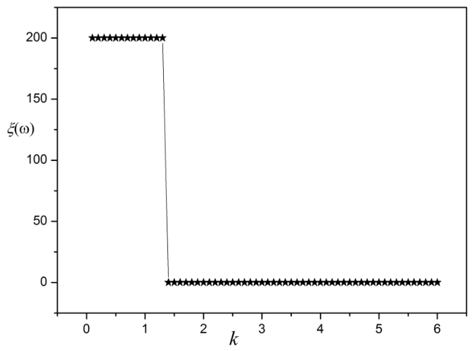
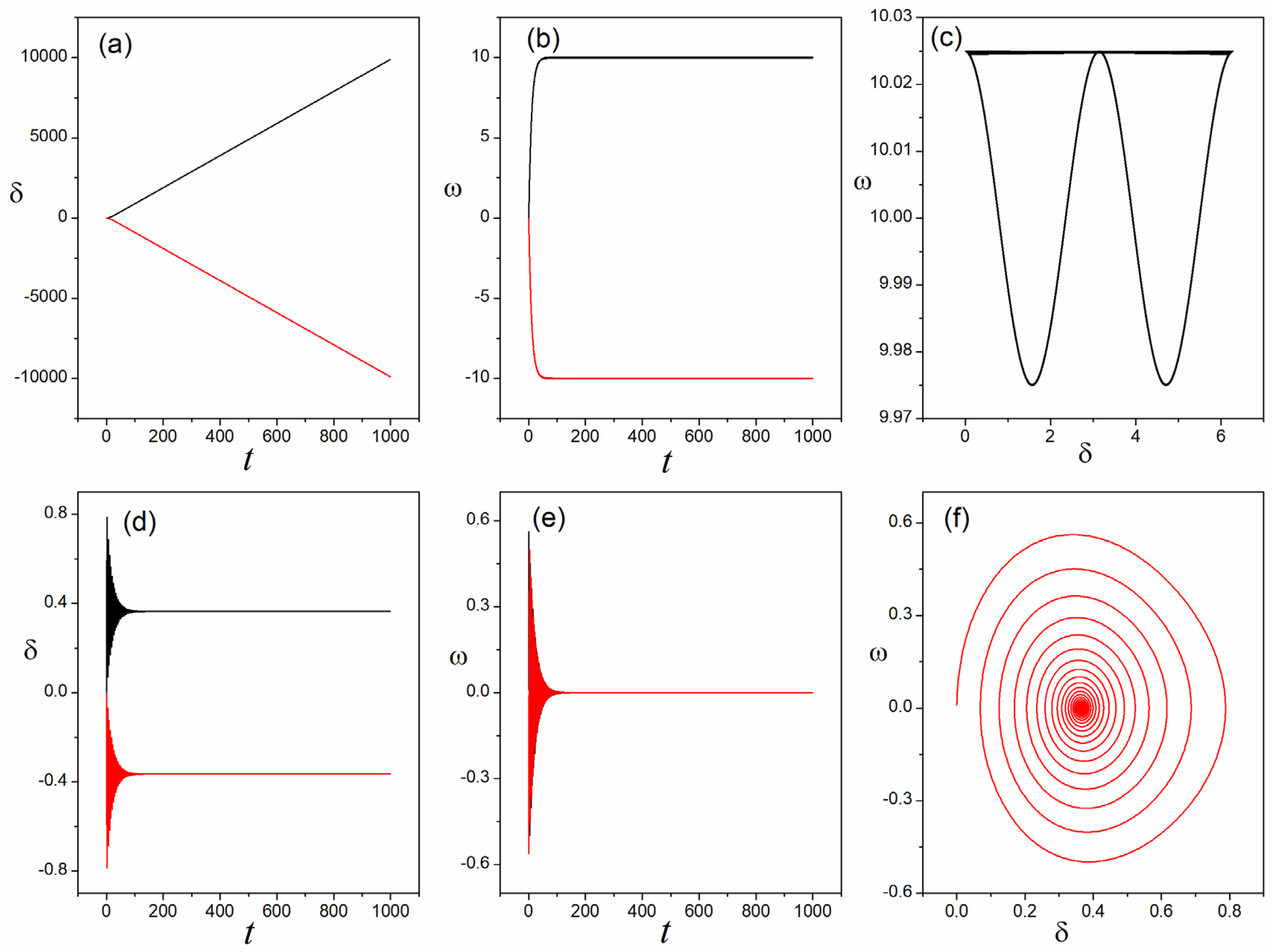
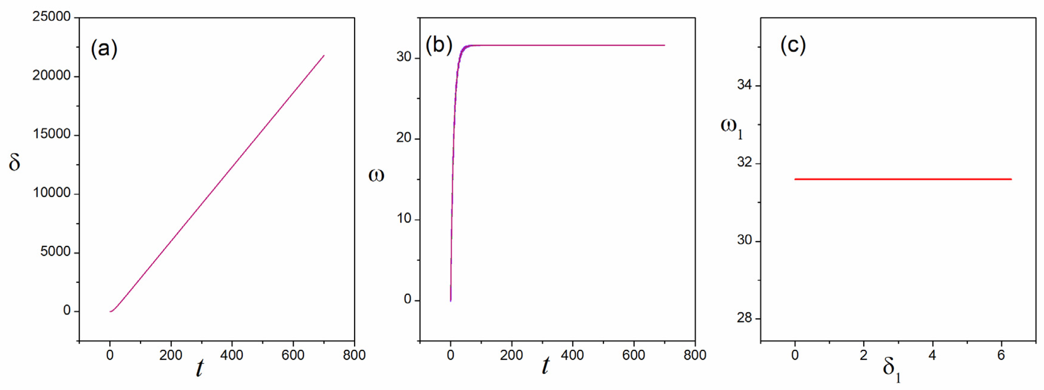
Firstly, the evolution of the error function ξ(ω) with increasing coupling intensity k is analyzed; the results are shown in Figure 1. It is confirmed that perfect frequency synchronization can be achieved when $k\ge 1.4$. This means that the critical coupling intensity of the network is k_c = 1.4 (i.e., at ξ(ω) ≈ 0). As a result, the time series of phase δ, angular frequency ω, and phase diagram for the sampled nodes with different parameters are calculated to show the dynamical behaviors of the power system; the results are shown in Figure 2a–f.

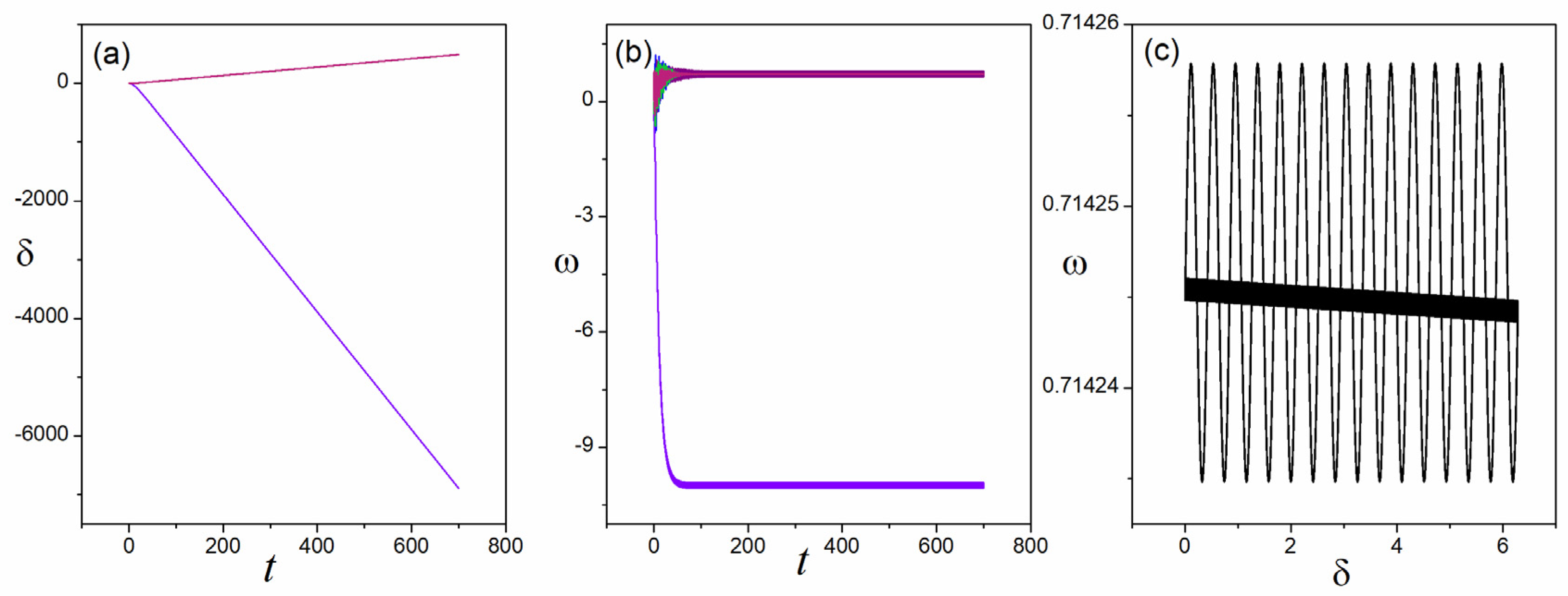
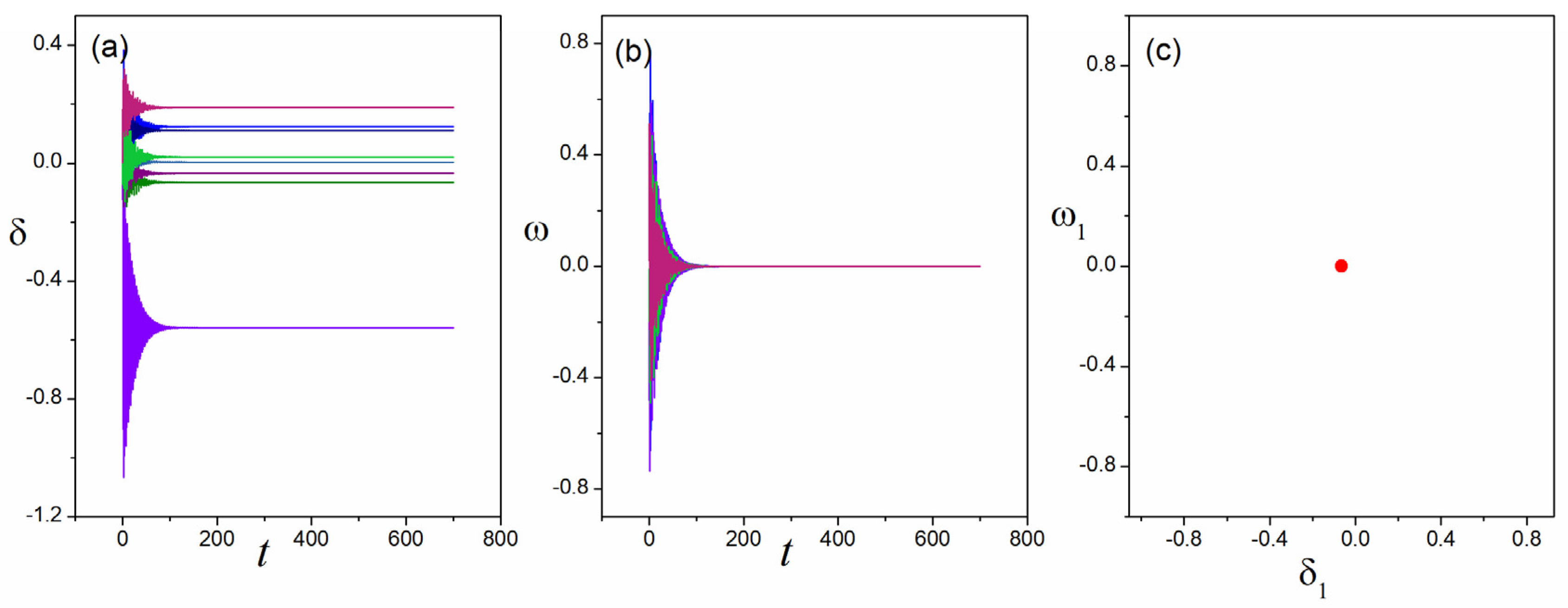
From Figure 2a–c, it can be seen that as time increases, the phase diverges while the angular frequency ω reaches a constant non-zero value. Also, the phase diagram shows a limit cycle, indicating desynchronization under these conditions. However, the results in Figure 2d–f show that with increasing time, the phase δ reaches a constant value while the angular frequency ω reaches zero. Also, the phase diagram is a fixed point, indicating that frequency synchronization is achieved. These results provide a good representation of the dynamic evolution characteristics in the power system with phase shift α = 0.

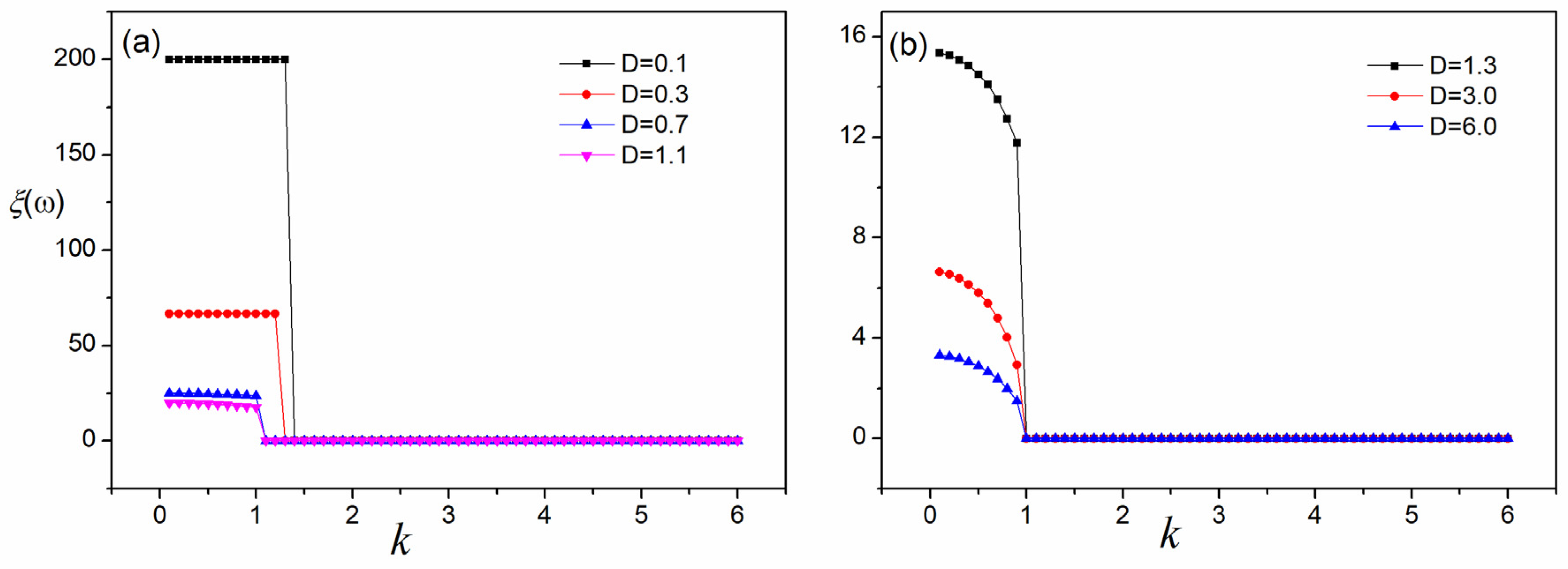
Furthermore, it is confirmed that the synchronization stability of a power system is also affected by damping. Hence, the variation in the error function ξ(ω) against the coupling intensity k is evaluated for different values of damping D. The results are shown in Figure 3. It can be seen that the intensity of the critical coupling k_c decreases with the increase in damping D as long as D < 1.3 and then remains constant. This means that critical damping exists and is equal to D_c = 1.3, that is, the system with small damping shows weak stability.

3.1.2. Phase Shift α ≠ 0

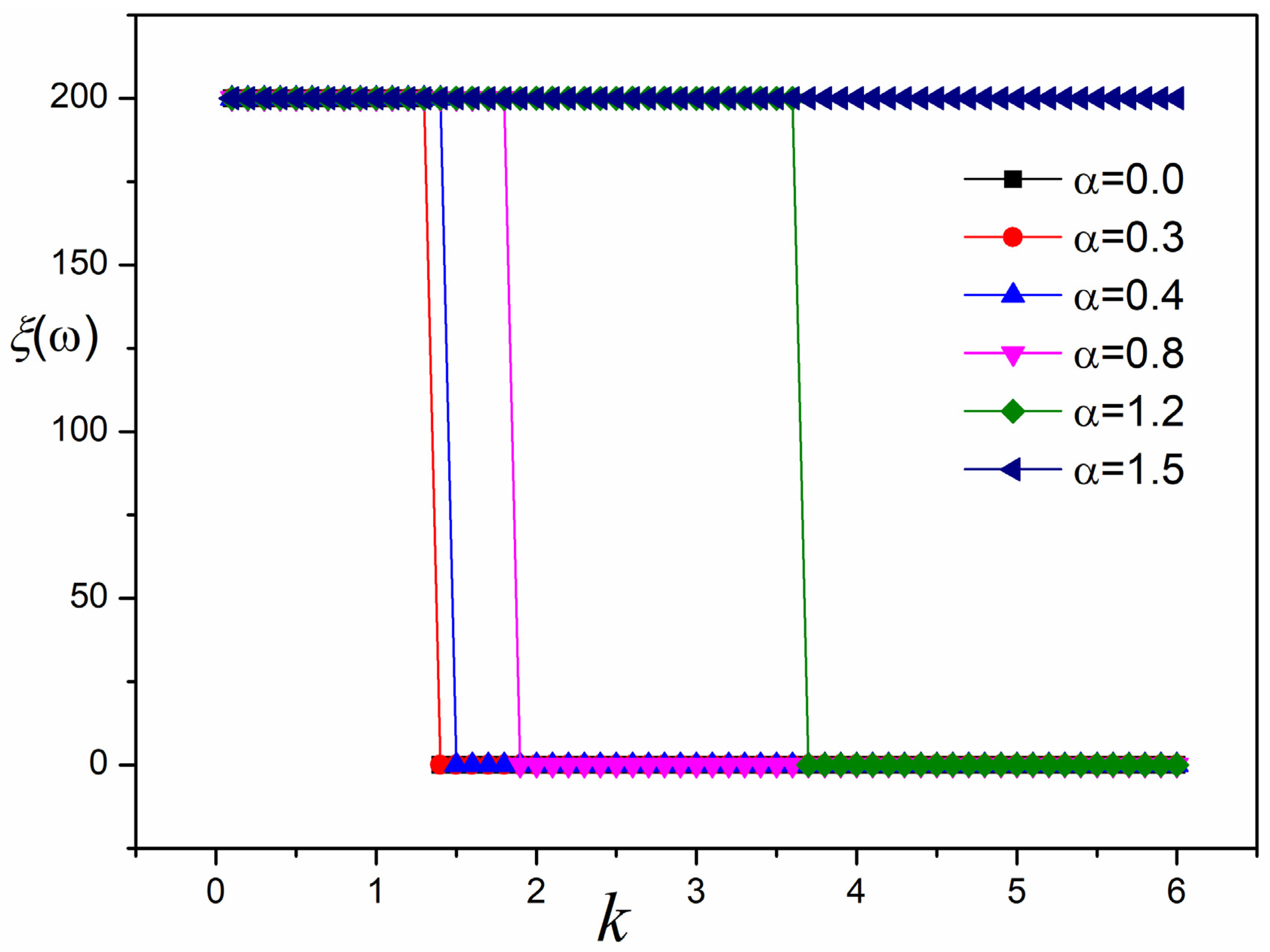
Based on the results shown above, the effect of phase shift (i.e., α ≠ 0) on the mode transition of collective dynamics in the power networks is discussed in the following. First, the value of the error function ξ(ω) is calculated for different coupling intensities k under different phase shift parameters α; the results are shown in Figure 4.

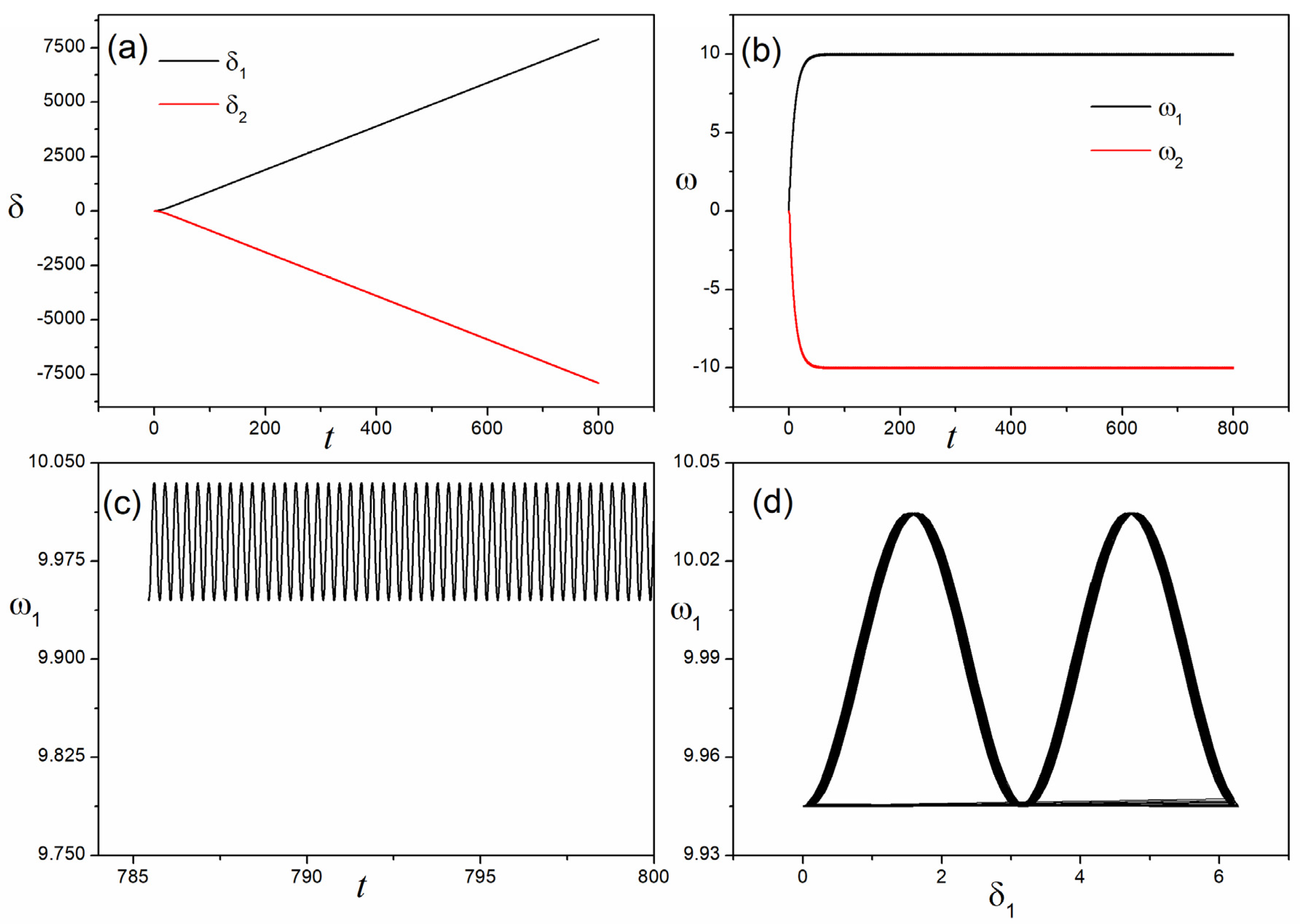
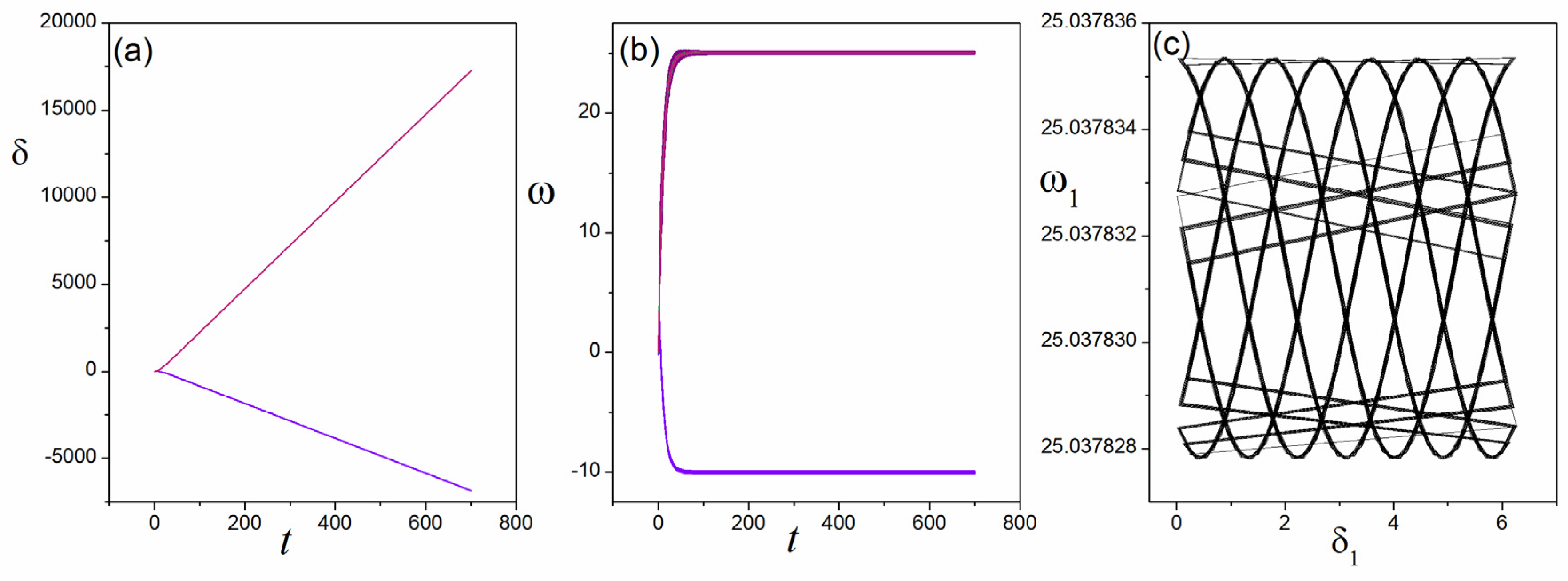
From Figure 4, it can be seen that the critical coupling intensity, k_c, increases with increasing phase shift. This means that the synchronization stability of the system depends on the phase shift parameter, and as the phase shift increases, the stability region of the system gradually decreases. Furthermore, it has been shown that the mode transition from synchronization to desynchronization can be detected in the network under the influence of a phase shift. Here, the time series and phase diagrams of the sampled nodes are calculated to explain the system’s dynamics; the results are plotted in Figure 5 and Figure 6.

From Figure 5, it is confirmed that the desynchronization state is detected, with the phase δ diverging and the angular frequency ω oscillating over time. Compared to the results shown in Figure 2a–c, it is interesting to note that the angular frequency ω is in a higher oscillation frequency state, which indicates that there is a mode transition from synchronization to desynchronization due to the phase shift.

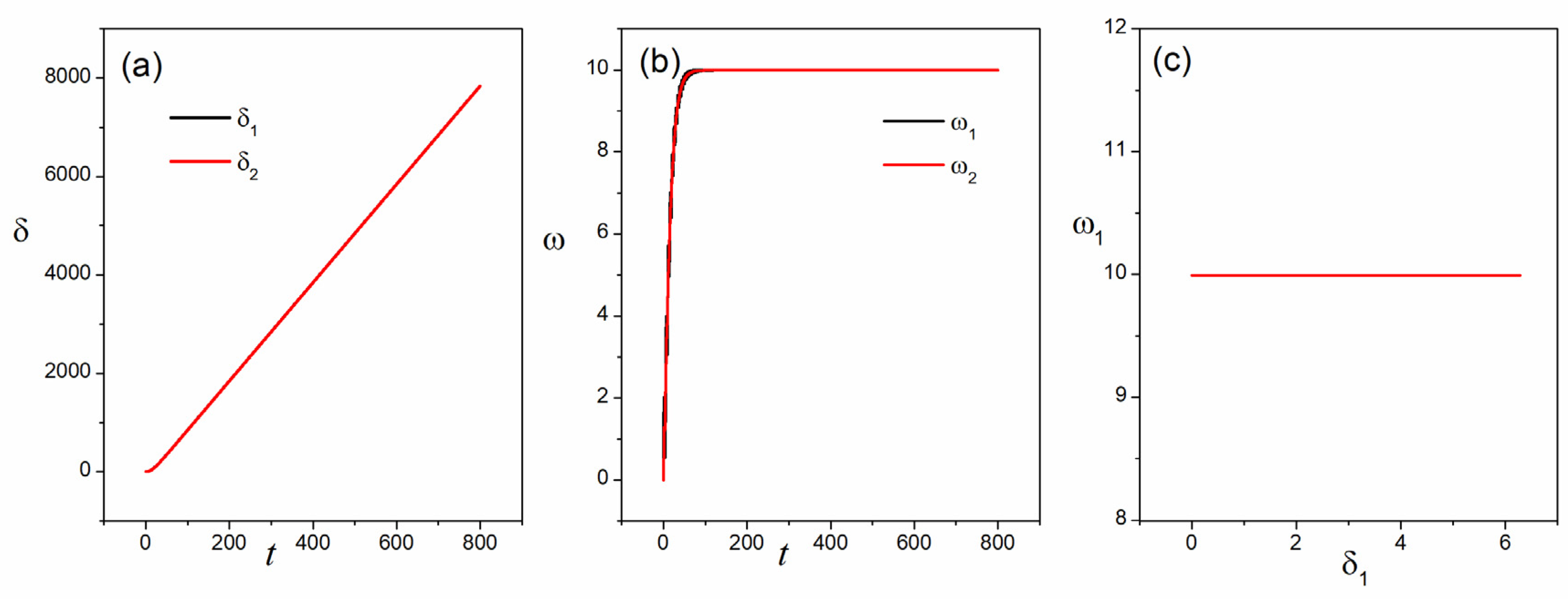
Furthermore, by taking the stable region parameters shown in Figure 4 (ξ(ω) ≈ 0), a new type of dynamic behavior, i.e., complete synchronization, is observed in the network, in which the phase δ of each node maintains the same step and the angular frequency ω reaches a constant value as time increases (see Figure 6). Compared with the results shown in Figure 2d–f, it is proved that the dynamical behaviors of the power network are completely changed by phase shift parameters, which change from frequency synchronization to complete synchronization.

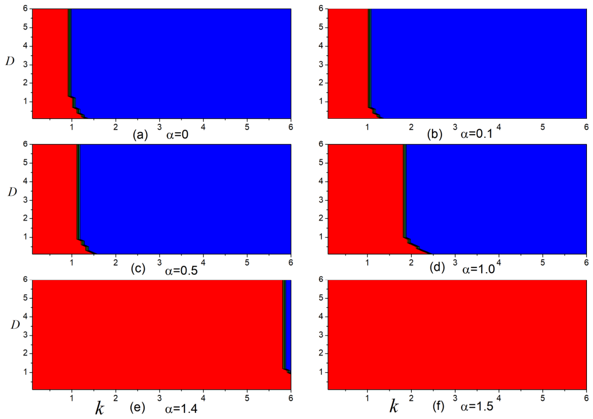
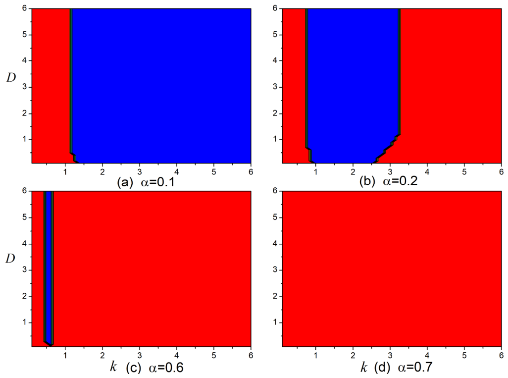
Based on these results, the distribution of system states in D–k phase space with different phase shifts α is calculated. The results are shown in Figure 7. From Figure 7, it can be seen that the synchronization stability region of the power network (blue region) continuously decreases with increasing phase shift α, and the synchronization state cannot be reached. Meanwhile, it is found that the dynamics of the system with small damping are more sensitive to phase shift and have little effect when choosing a small phase shift parameter (α ≤ 0.3).

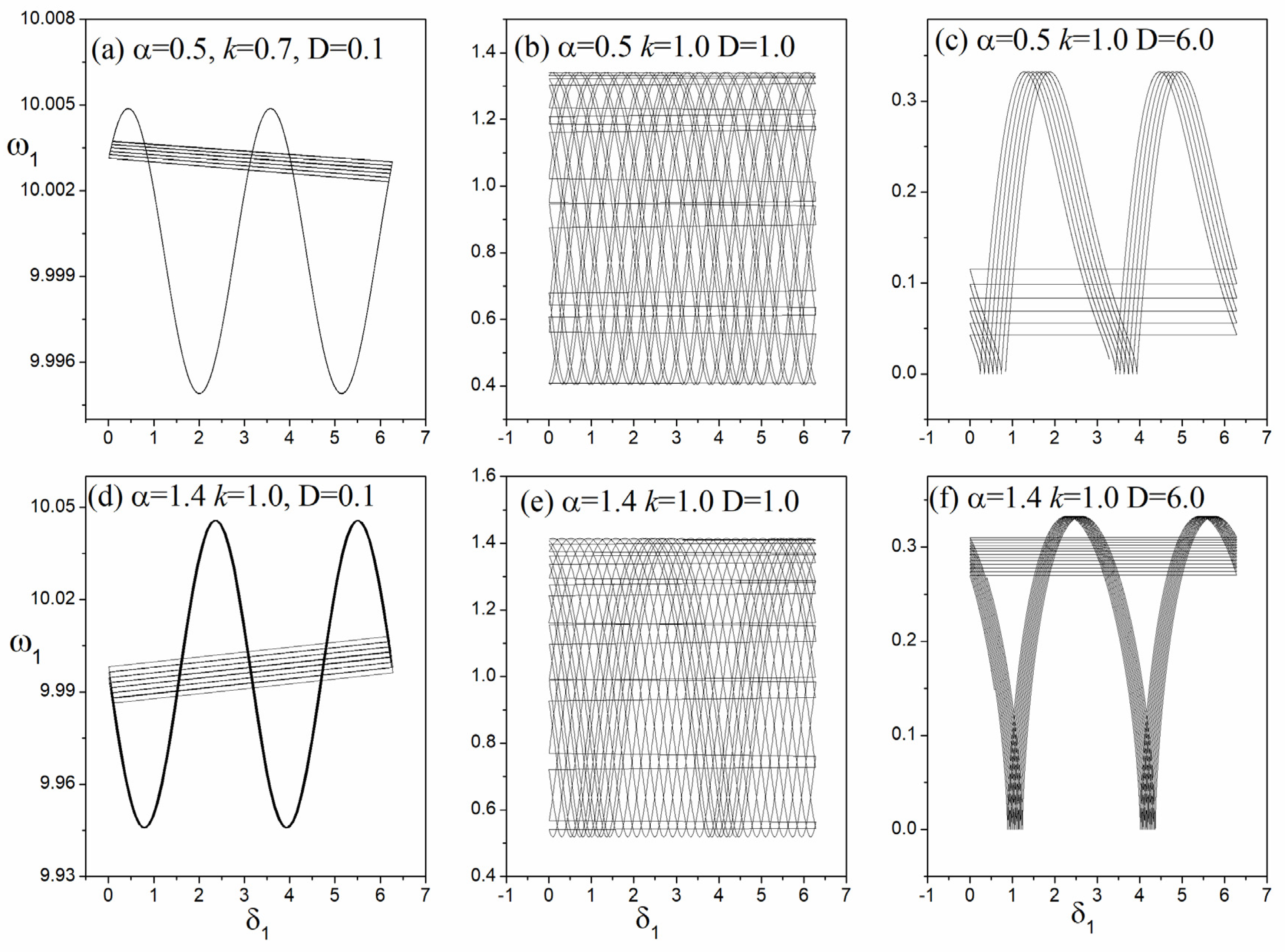
In addition, a large number of simulations have been performed, yielding other interesting results. For example, as shown in Figure 8, different phase diagrams can be identified in the unstable region under different parameter selections.

All these results indicate that the two-node power system exhibits much more complex dynamics than the single-machine power system, due to the phase-shift parameter [42]. Consequently, it is necessary to quantitatively analyze the changes in stability of the power system under the influence of phase-shift parameters and to explore the mechanism by which the system loses stability.

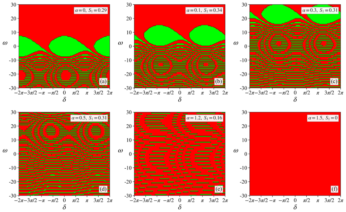
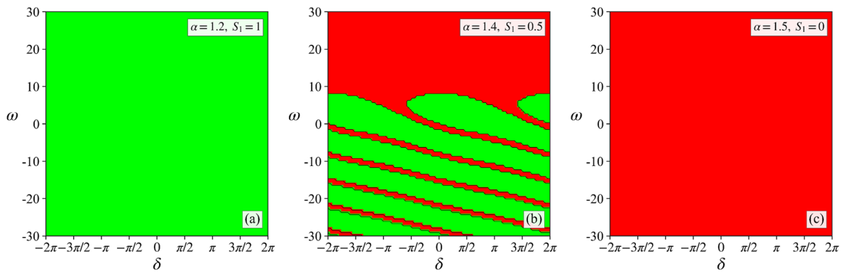
Next, we will quantitatively analyze changes in system stability under the effect of the phase-shift parameter by calculating basin stability. To better present the results, we will separately compute the basin stability for the power system with small damping and for the power system with large damping; the results are plotted in Figure 9 and Figure 10. Here, the number of initial value vectors, T = 2500, that is, δ₀ and ω₀, are randomly drawn from box B = [δ_s − 2π, δ_s + 2π] × [−100, 100].

Figure 9 and Figure 10 show the basin stability results for a generator with different phase-shift parameter α values, with damping D = 0.1 and D = 1, respectively. It is interesting to find in Figure 9 that the stability region (or basin of attraction) moves progressively to larger phase differences as the phase-shift parameter α increases. For instance, at α = 0.1, the system exhibits a finite stability measure (S₁ = 0.34); however, as α is raised to 1.5, the stability measure drops to zero, indicating that the stable operating point has shifted outside the physically meaningful range. That is why the stability region of the power system reduces with the increasing phase shift. This migration of the stability region reflects the deteriorating effect of line losses on synchronization.

Furthermore, the basin stability for a generator with large damping (D = 1) is calculated, and the results are shown in Figure 10. It can be confirmed that the same results are obtained in Figure 10. As the phase-shift parameter increases, the basin of attraction gradually shifts to larger phase separations and eventually disappears entirely beyond a critical threshold. However, a large damping coefficient endows the system with strong stability, making it relatively insensitive to changes in the phase shift parameter. This result not only provides a quantitative analysis of changes in power system stability but also offers strong evidence for the results presented in Figure 7.

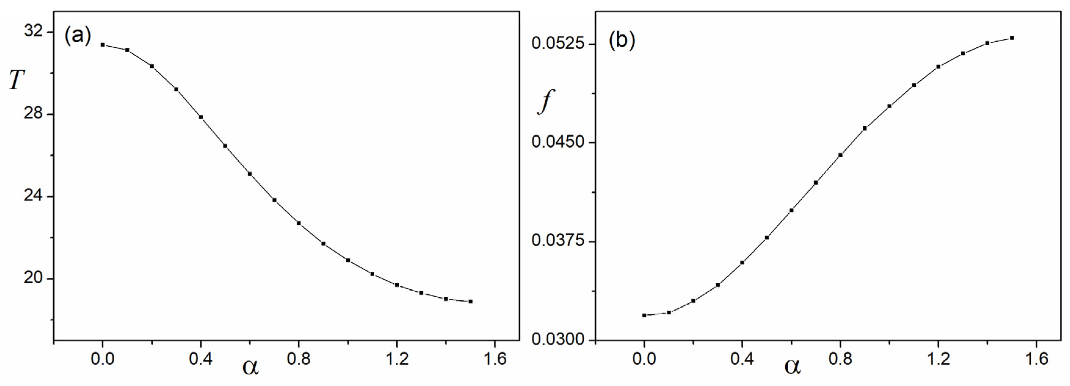
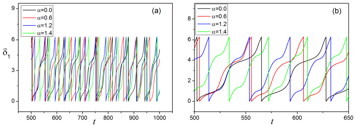
In other words, the results reveal the mechanism by which the system loses stability under the effect of the phase-shift parameter. Therefore, the oscillation period T, the oscillation frequency f of the angular frequency ω, and phase δ with different phase shifts α are calculated to give the answer; the results are shown in Figure 11 and Figure 12.

In Figure 11, the oscillation period T and the oscillation frequency f are calculated for the angular frequency ω with different phase shifts α. The results show that the oscillation period T of angular frequency ω decreases as the phase shift increases (i.e., the oscillation frequency f increases). This means that the larger the phase shift parameter α, the higher the angular frequency ω. Moreover, it is proved in Figure 12 that the phase difference manifests between phase δ of distinct nodes in a power network while different phase shifts (line resistance) α are selected. That is why, under the effect of the phase shift parameter, the system’s stable operating point shifts outside the physically meaningful range and then loses stability.

In summary, it is confirmed that interesting and distinct results are observed in the two-node power system due to the phase shift. The conclusions are as follows: (1) Complete synchronization, rather than frequency synchronization, is detected in the power network. (2) The larger the phase shift, the more sensitive the stability of the power network is, and it can completely lose stability. (3) The basin stability is calculated and quantitatively analyzes the system stability changes, and then provides the underlying mechanism for the power system to lose stability due to the effect of the phase shift parameter.

3.2. Case II Nepal Power Network

In this section, the more complex Nepal power network, consisting of a 15-node network, will be used for further discussion. Here, the evolution of dynamical behaviors and the stability of the power system with different phase shifts are also analyzed.

At first, the time series of phase δ and angular frequency ω of the power network are calculated with phase shift α = 0, and the results are shown in Figure 13 and Figure 14.

The results in Figure 13 and Figure 14 show the characteristics of the dynamic evolution of nodes in desynchronization and synchronization states in a power network with appropriately selected parameters. The results show that frequency synchronization is induced in the power network with a phase shift α = 0.

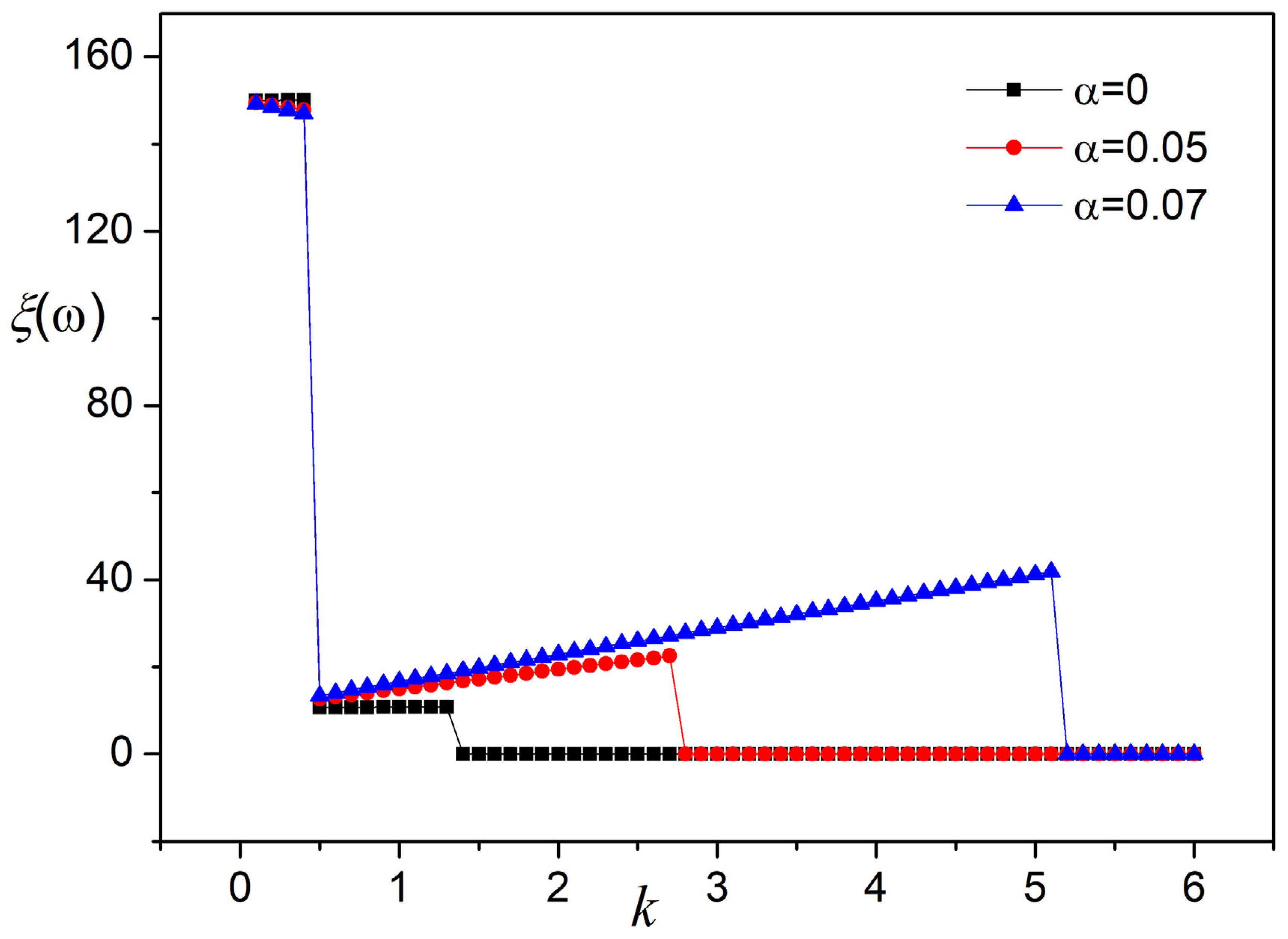
Based on this, the variation in error function ξ(ω) against the coupling intensity k is also evaluated for different phase shifts α, and the results are plotted in Figure 15.

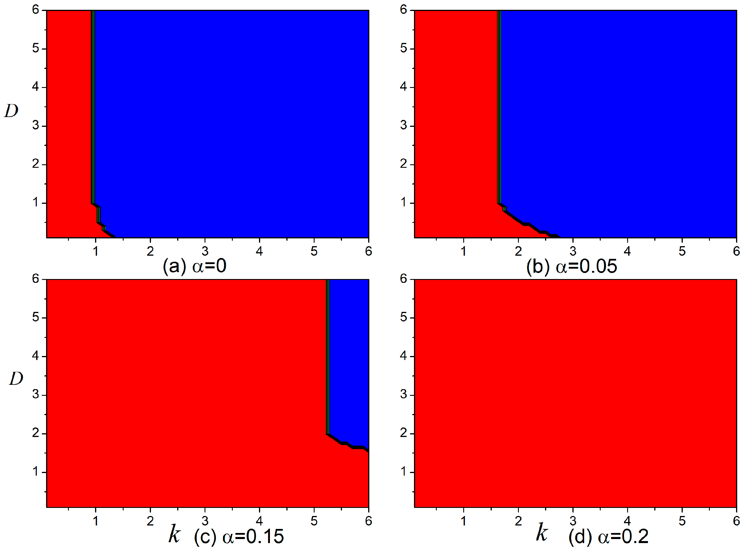
Interestingly, Figure 15 shows that the critical coupling intensity k_c increases significantly with increasing phase shift, even for very small phase shifts. This means that the stability of the more complex power network is more sensitive to the phase shift parameter α. As a result, the state distribution of power grids in the D–k phase space with different phase shifts is also calculated, and the results are shown in Figure 16.

As shown in Figure 16, the instability region of the network expands with increasing phase shift and becomes completely unstable at a small phase shift. Compared to a two-node power network, the results show that the stability of the Nepal power network is much more sensitive to phase shifts. Here, the time series is computed for the sampled nodes in the power network to investigate whether other dynamic behaviors occur. The results are shown in Figure 17 and Figure 18. According to these figures, complete synchronization and diverse desynchronization dynamical behaviors can be observed in the stable and unstable regions, respectively, as in the two-node power system.

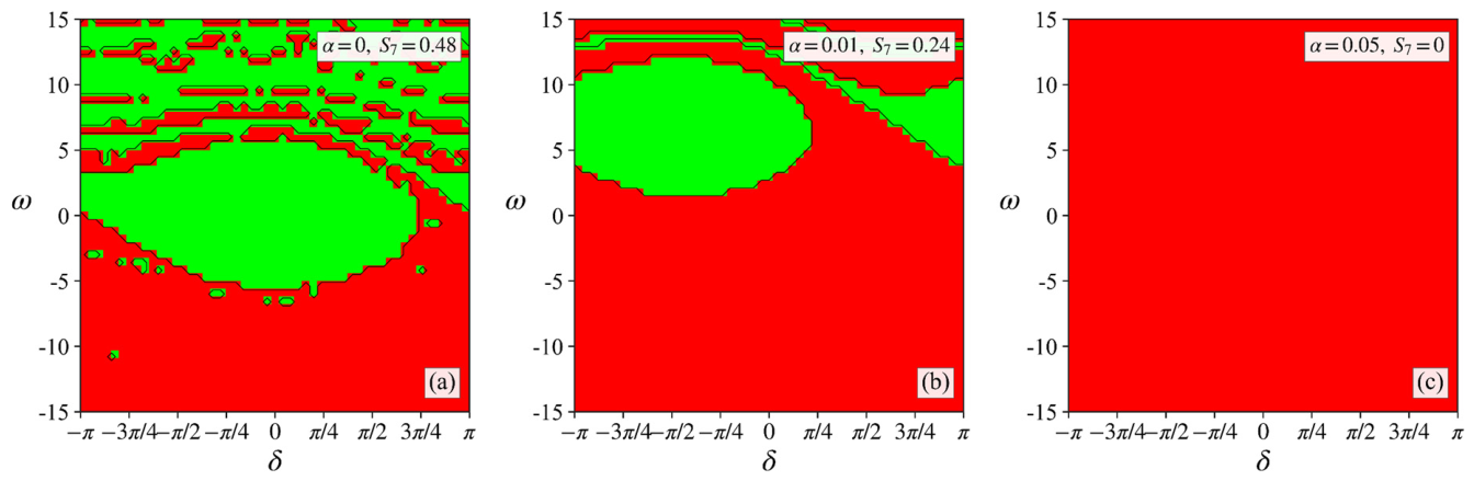
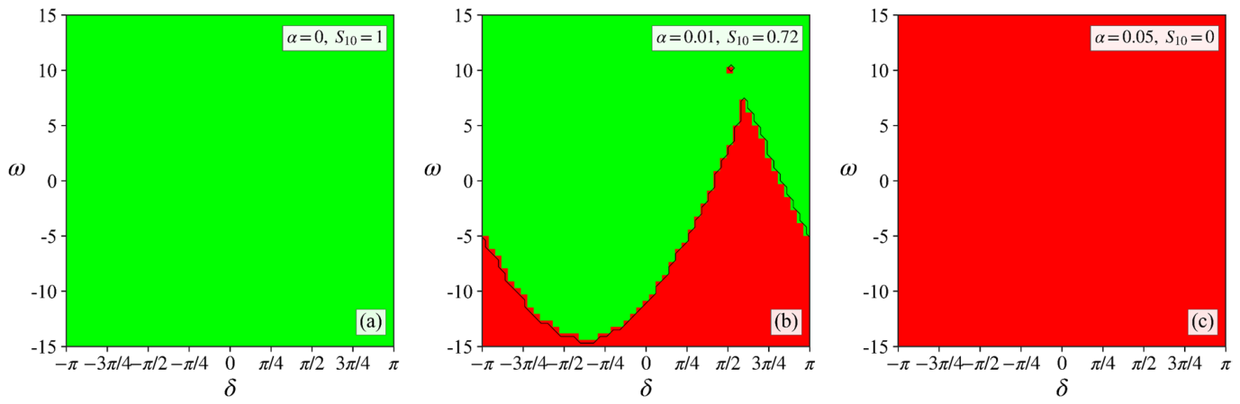
In this section, the basin stability of the power system is also calculated to quantitatively analyze changes in system stability, which are affected by phase shift parameters. To better present the results, the basin stability S_i for nodes with different degrees in the power network is calculated, and the results are plotted in Figure 19 and Figure 20. Here, the number of initial value vectors, T = 2500, that is, δ₀ and ω₀, are randomly drawn from box B = [δ_s − 2π, δ_s + 2π] × [−100, 100].

Figure 19 and Figure 20 show the results of basin stability for different nodes with different phase-shift parameters α selected, with nodes n = 7 (smallest degree = 1) and n = 10 (largest degree = 13), respectively.

As shown in Figure 19, the results are similar to those in Figure 9, with the stability region (or basin of attraction) moving progressively to larger phase differences as the phase-shift parameter α increases. It is interesting to note that as α is raised to 0.05, the stability measure drops to zero, indicating that the stable operating point has shifted outside the physically meaningful range, with a very small phase shift.

Furthermore, the basin stability for nodes with the largest degree is also calculated; the results are shown in Figure 20. It is found that though nodes with large degrees possess comparatively broader stability domains, their stability is eventually lost as the phase shift parameter increases, and the values are very small. These results show that the stability of the power system is sensitive to network size under the effect of phase shift and provide good evidence for the results shown in Figure 16.

More importantly, this result elucidates the mechanism by which the system loses stability under the influence of the phase-shift parameter.

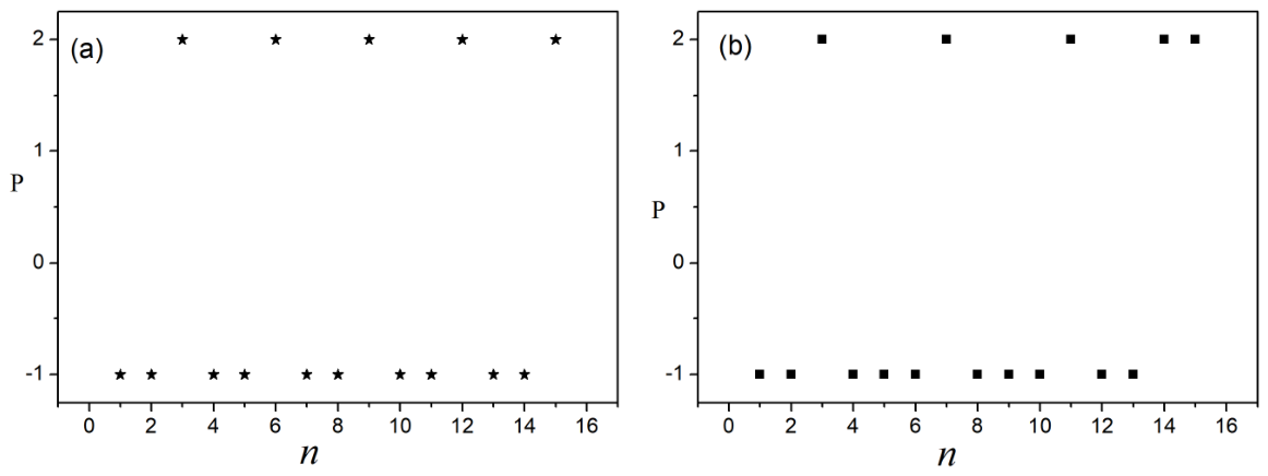
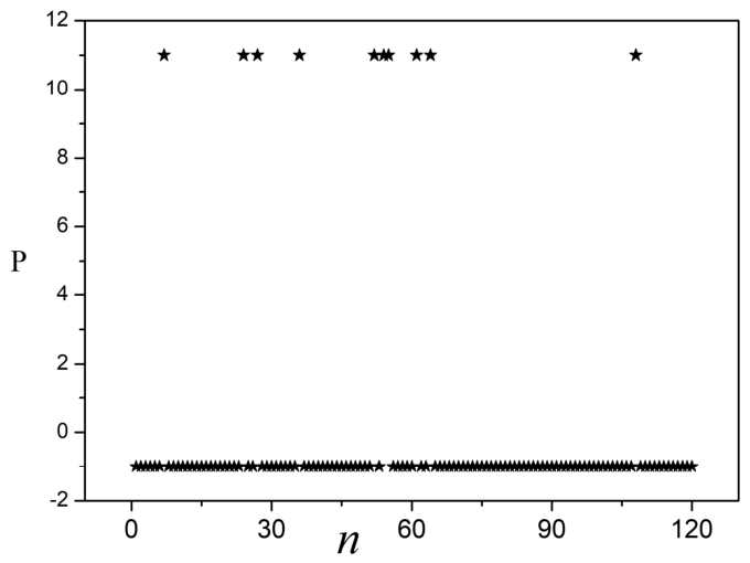
In fact, an interesting thing to note is that the stability of the complex power network can also be affected by the distribution of nodes (generators and consumers) in the network. That is, the instability area’s growth process can exhibit different evolutions with increasing phase shift (see Figure 21).

Compared with the results shown in Figure 16, Figure 21 confirms that although the power system’s stability region decreases with increasing phase shift, the evolutionary behavior differs. The reason is that the change in the distribution of generator locations in the power network, as shown in Figure 22, results in a need to further explore the relationship between system stability changes and the distribution of nodes. It can be concluded that the dynamical behavior in the much more complex network is affected by additional factors, which will be interesting to investigate further.

3.3. Case III UK Power Network

As shown above, the results indicate that the power system’s stability is sensitive to phase shifts, and the transition from frequency synchronization to complete synchronization can be induced by it. Hence, the case of a larger power system, the UK power network, which consists of 120 nodes, is discussed to explore whether this result is universally applicable.

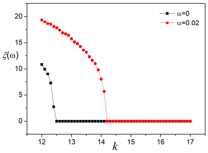
At first, the evolution of the error function ξ(ω) of the power system with different phase shifts is calculated to show changes in synchronization stability, which are shown in Figure 23. Interestingly, it is proved that the critical coupling strength of the system increases significantly. In contrast, a very small phase shift parameter is selected.

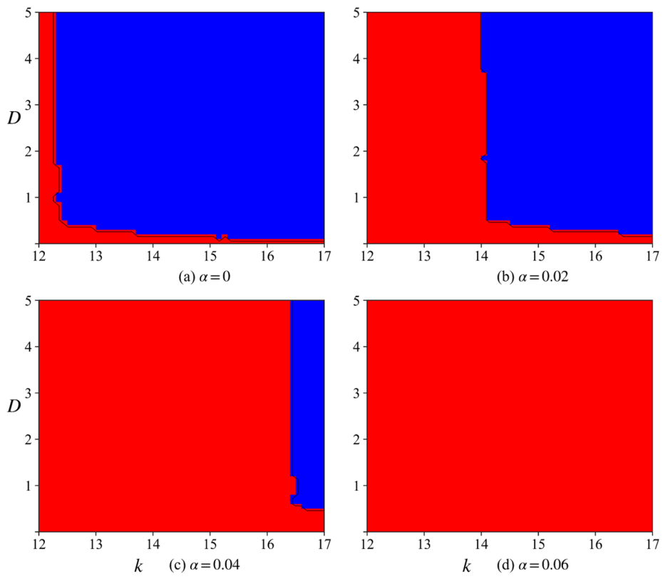
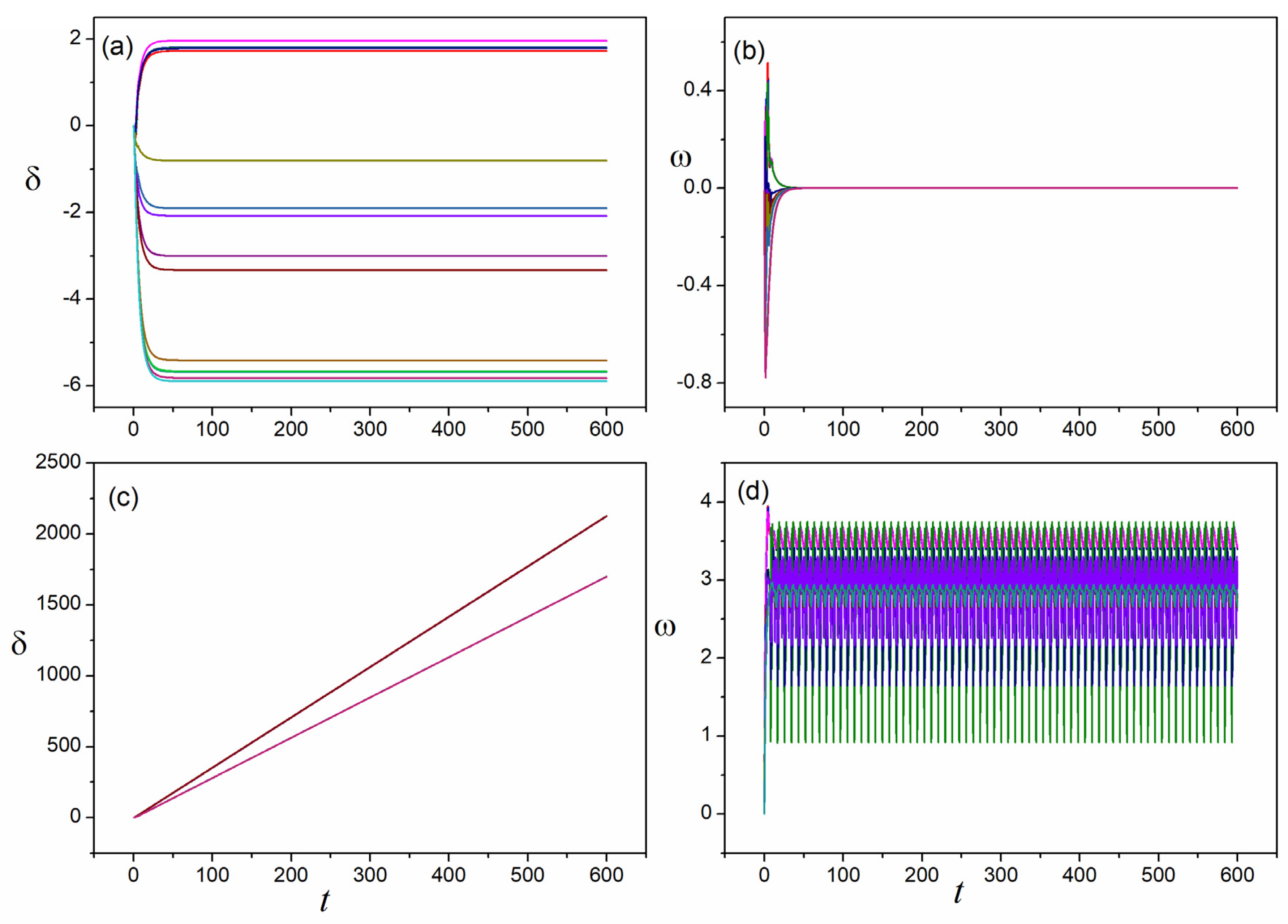
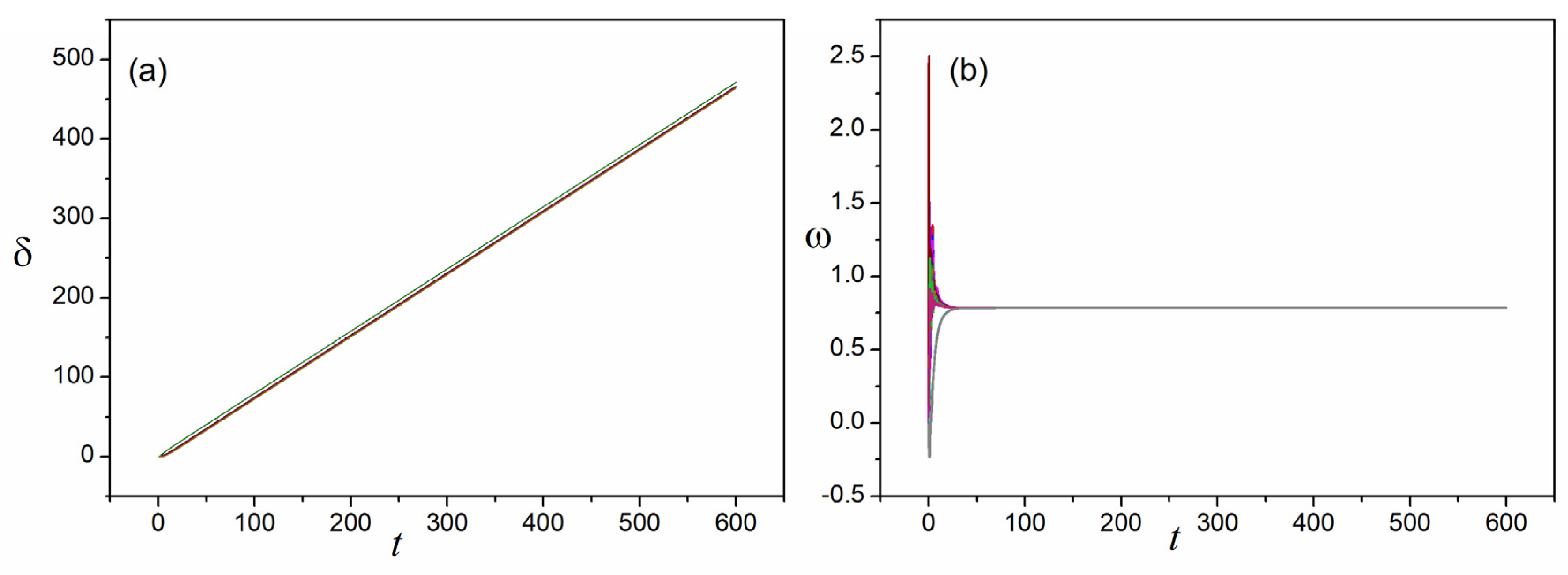
Therefore, the state distribution in the D–k phase space with different phase shifts is also calculated to give the overall evolutionary characteristics and synchronization stability of the power system, shown in Figure 24. The node distribution in the network is plotted in Figure 25. It is confirmed that the stability region decreases with increasing phase shift. The system completely loses synchronization with a very small α of 0.06. Combining the results shown in Figure 7, Figure 16, and Figure 24, it is shown that the system’s stability is sensitive to the network size under the effect of the phase shift parameter. Furthermore, the results indicate that complete synchronization, rather than frequency synchronization, can be induced in the stable region due to the effect of phase shift, as shown in Figure 26 and Figure 27.

4. Conclusions

In the modern era, power grids are becoming increasingly large and complex, resulting in more complicated collective dynamics and stability behaviors due to the significant manifestation of symmetry-breaking in the power network. Therefore, it is of great significance and necessity to continuously investigate the dynamics and stability of lossy power networks from various perspectives.

In this paper, the effects of phase-shift parameters, which represent ohmic losses in transmission lines, on the dynamics and stability of power networks with different sizes and topological structures are systematically investigated. In the study, three representative power networks are considered: a two-node power network (one generator and one consumer), the Nepal power network (15 nodes), and the UK power network (120 nodes) to demonstrate changes in network size and topological structure. Moreover, the error function and basin stability are calculated to qualitatively and quantitatively analyze the system dynamics and stability.

The results indicate that a variety of interesting dynamical behaviors can emerge in power networks under the influence of phase shift, compared with the conventional single-machine power system [42]. Firstly, complete synchronization rather than frequency synchronization can be induced in the network due to phase shifts. These different synchronization behaviors can be interpreted as transitions between different dynamical symmetry states in complex power networks. Secondly, the stability of the power network is strongly influenced by phase-shift parameters, and the stability evolution shows significant sensitivity to network scale, topological structure, damping, and node spatial distribution. It can be concluded that (1) the unstable region of the power network continuously expands with increasing phase shift; (2) the synchronization stability becomes increasingly sensitive to phase shift as the network size increases; and (3) the stability of the power system is significantly affected by the spatial distribution of generators and consumers in the network. These results reflect the deteriorating effect of line losses on synchronization. In other words, these results confirm that line losses can systematically reduce the stability region and ultimately destroy synchrony in power networks.

Furthermore, the results for basin stability not only quantitatively analyze the changes in system stability under the effect of the phase shift parameter but also reveal the mechanism underlying the loss of stability, namely, the shift in the stable operating point outside the physically meaningful range. Of course, it is proven that the system’s stable operating point shifts outside the physically meaningful range because the phase-shift parameter not only intensifies frequency oscillations but also induces phase differences between nodes in the power network.

It can be seen that the more pronounced the symmetry-breaking in a power network, the more significant the effect of the phase-shift parameter on the network’s dynamics and stability. The insights obtained in this paper are meaningful for further studies on synchronization dynamics, operation, and design of complex power systems.

5. Open Problem

While the present study provides fundamental insights into the effect of the phase-shift parameter on synchronization and stability within the widely adopted oscillator-based power network framework, several important open questions remain to be addressed in future investigations. For example, the mechanism underlying the transition from frequency synchronization to competitive synchronization should be explored and subjected to theoretical analysis; then, the relationships among node distribution, network stability, and phase-shift parameters should be investigated and quantitatively analyzed. Moreover, the heterogeneity of damping, inertia, transmission lines, and voltage variations should be considered in further studies to better align the research with the characteristics of actual power networks and ensure that the results are applicable to real power grids.

References

1. Abedi, A.; Gaudard, L.; Romerio, F. Review of major approaches to analyze vulnerability in power system. Reliab. Eng. Syst. Saf. 2019, 183, 153–172. [Google Scholar] [CrossRef]
2. Zio, E.; Aven, T. Uncertainties in smart grids behavior and modeling: What are the risks and vulnerabilities? How to analyze them? Energy Policy 2011, 39, 6308–6320. [Google Scholar] [CrossRef]
3. Olmi, S.; Gambuzza, L.V.; Frasca, M. Multilayer control of synchronization and cascading failures in power grids. Chaos Solitons Fractals 2024, 180, 114412. [Google Scholar] [CrossRef]
4. Ajjarapu, V.A.B.L.; Lee, B. Bifurcation theory and its application to nonlinear dynamical phenomena in an electrical power system. IEEE Trans. Power Syst. 2002, 7, 424–431. [Google Scholar]
5. Arapostathis, A.; Sastry, S.; Varaiya, P. Global analysis of swing dynamics. IEEE Trans. Circuits Syst. 2003, 29, 673–679. [Google Scholar]
6. Demello, F.P.; Concordia, C. Concepts of synchronous machine stability as affected by excitation control. IEEE Trans. Power Appar. Syst. 1969, 88, 316–329. [Google Scholar] [CrossRef]
7. Paganini, F.; Lesieutre, B.C. Generic properties, one-parameter deformations, and the BCU method [power system stability]. IEEE Trans. Circuits Syst. I Fundam. Theory Appl. 2002, 46, 760–763. [Google Scholar]
8. Chiang, H.D. Direct Methods for Stability Analysis of Electric Power Systems: Theoretical Foundation, BCU Methodologies, and Applications; John Wiley & Sons: Hoboken, NJ, USA, 2011. [Google Scholar]
9. Filatrella, G.; Nielsen, A.H.; Pedersen, N.F. Analysis of a power grid using a Kuramoto-like model. Eur. Phys. J. B 2008, 61, 485–491. [Google Scholar] [CrossRef]
10. Ma, J.; Sun, Y.; Yuan, X.; Kurths, J.; Zhan, M. Dynamics and collapse in a power system model with voltage variation: The damping effect. PLoS ONE 2016, 11, e0165943. [Google Scholar] [CrossRef] [PubMed]
11. Yousef, A.M.; Kassem, A.M. Optimal power system stabilizer-based enhancement of synchronizing and damping torque coefficients. In WSEAS Transactions on Power Systems; WSEAS: Athens, Greece, 2012. [Google Scholar]
12. Dorogovtsev, S.N.; Goltsev, A.V.; Mendes, J.F. Critical phenomena in complex networks. Rev. Mod. Phys. 2008, 80, 1275–1335. [Google Scholar] [CrossRef]
13. Hu, G.; Hu, J.; Kang, K.; Xu, X.; Ren, Y. Identifying important nodes based on neighborhood multi order multi attribute in complex networks. Phys. Scr. 2025, 100, 055211. [Google Scholar] [CrossRef]
14. Pagani, G.A.; Aiello, M. The power grid as a complex network: A survey. Phys. A Stat. Mech. Its Appl. 2013, 392, 2688–2700. [Google Scholar] [CrossRef]
15. Forsberg, S.; Thomas, K.; Bergkvist, M. Power grid vulnerability analysis using complex network theory: A topological study of the Nordic transmission grid. Phys. A Stat. Mech. Its Appl. 2023, 626, 129072. [Google Scholar] [CrossRef]
16. Shahpari, A.; Khansari, M.; Moeini, A. Vulnerability analysis of power grid with the network science approach based on actual grid characteristics: A case study in Iran. Phys. A Stat. Mech. Its Appl. 2019, 513, 14–21. [Google Scholar] [CrossRef]
17. Costa, L.D.F.; Oliveira, O.N., Jr.; Travieso, G.; Rodrigues, F.A.; Villas Boas, P.R.; Antiqueira, L.; Viana, M.P.; Correa Rocha, L.E. Analyzing and modeling real-world phenomena with complex networks: A survey of applications. Adv. Phys. 2011, 60, 329–412. [Google Scholar] [CrossRef]
18. Dörfler, F.; Chertkov, M.; Bullo, F. Synchronization in complex oscillator networks and smart grids. Proc. Natl. Acad. Sci. USA 2013, 110, 2005–2010. [Google Scholar] [CrossRef] [PubMed]
19. Zou, Y.; Wang, R.; Gao, Z. Improve synchronizability of a power grid through power allocation and topology adjustment. Phys. A Stat. Mech. Its Appl. 2020, 548, 122956. [Google Scholar] [CrossRef]
20. Motter, A.E.; Myers, S.A.; Anghel, M.; Nishikawa, T. Spontaneous synchrony in power-grid networks. Nat. Phys. 2013, 9, 191–197. [Google Scholar] [CrossRef]
21. Bergen, A.R.; Hill, D.J. A structure preserving model for power system stability analysis. IEEE Trans. Power Appar. Syst. 1981, 100, 25–35. [Google Scholar] [CrossRef]
22. Lozano, S.; Buzna, L.; Díaz-Guilera, A. Role of network topology in the synchronization of power systems. Eur. Phys. J. B 2012, 85, 231. [Google Scholar] [CrossRef]
23. Nishikawa, T.; Motter, A.E. Comparative analysis of existing models for power-grid synchronization. New J. Phys. 2015, 17, 015012. [Google Scholar] [CrossRef]
24. Dorfler, F.; Bullo, F. Kron reduction of graphs with applications to electrical networks. IEEE Trans. Circuits Syst. I Regul. Pap. 2012, 60, 150–163. [Google Scholar] [CrossRef]
25. Epstein, I.R.; Showalter, K. Nonlinear chemical dynamics: Oscillations, patterns, and chaos. J. Phys. Chem. 1996, 100, 13132–13147. [Google Scholar] [CrossRef]
26. Yuan, D.; Zhang, M.; Yang, J. Dynamics of the Kuramoto model in the presence of correlation between distributions of frequencies and coupling strengths. Phys. Rev. E 2014, 89, 012910. [Google Scholar] [CrossRef]
27. Acebrón, J.A.; Spigler, R. Adaptive frequency model for phase-frequency synchronization in large populations of globally coupled nonlinear oscillators. Phys. Rev. Lett. 1998, 81, 2229. [Google Scholar] [CrossRef]
28. Trees, B.R.; Saranathan, V.; Stroud, D. Synchronization in disordered Josephson junction arrays: Small-world connections and the Kuramoto model. Phys. Rev. E 2005, 71, 016215. [Google Scholar] [CrossRef]
29. Dorfler, F.; Bullo, F. Synchronization and transient stability in power networks and nonuniform Kuramoto oscillators. SIAM J. Control Optim. 2012, 50, 1616–1642. [Google Scholar] [CrossRef]
30. Zhang, J.; Boccaletti, S.; Liu, Z.; Guan, S. Synchronization of phase oscillators under asymmetric and bimodal distributions of natural frequencies. Chaos Solitons Fractals 2020, 136, 109777. [Google Scholar] [CrossRef]
31. Boccaletti, S.; Almendral, J.A.; Guan, S.; Leyva, I.; Liu, Z.; Sendiña-Nadal, I.; Wang, Z.; Zou, Y. Explosive transitions in complex networks’ structure and dynamics: Percolation and synchronization. Phys. Rep. 2016, 660, 1–94. [Google Scholar] [CrossRef]
32. Khramenkov, V.; Dmitrichev, A.; Nekorkin, V. Partial stability criterion for a heterogeneous power grid with hub structures. Chaos Solitons Fractals 2021, 152, 111373. [Google Scholar] [CrossRef]
33. Lacerda, J.C.; Freitas, C.; Macau, E.E. Elementary changes in topology and power transmission capacity can induce failures in power grids. Phys. A Stat. Mech. Its Appl. 2022, 590, 126704. [Google Scholar] [CrossRef]
34. Witthaut, D.; Timme, M. Braess’s paradox in oscillator networks, desynchronization and power outage. New J. Phys. 2012, 14, 083036. [Google Scholar]
35. Witthaut, D.; Timme, M. Nonlocal failures in complex supply networks by single link additions. Eur. Phys. J. B 2013, 86, 377. [Google Scholar] [CrossRef]
36. Menck, P.J.; Heitzig, J.; Kurths, J.; Joachim Schellnhuber, H. How dead ends undermine power grid stability. Nat. Commun. 2014, 5, 3969. [Google Scholar] [CrossRef] [PubMed]
37. Schultz, P.; Heitzig, J.; Kurths, J. Detours around basin stability in power networks. New J. Phys. 2014, 16, 125001. [Google Scholar] [CrossRef]
38. Rohden, M.; Sorge, A.; Witthaut, D.; Timme, M. Impact of network topology on synchrony of oscillatory power grids. Chaos 2014, 24, 013123. [Google Scholar] [CrossRef] [PubMed]
39. Rohden, M.; Sorge, A.; Timme, M.; Witthaut, D. Self-organized synchronization in decentralized power grids. Phys. Rev. Lett. 2012, 109, 064101. [Google Scholar] [CrossRef] [PubMed]
40. Xi, Z.; Feng, G.; Cheng, D.; Lu, Q. Nonlinear decentralized saturated controller design for power systems. IEEE Trans. Control Syst. Technol. 2003, 11, 539–547. [Google Scholar]
41. Arinushkin, P.A.; Vadivasova, T.E. Nonlinear damping effects in a simplified power grid model based on coupled Kuramoto-like oscillators with inertia. Chaos Solitons Fractals 2021, 152, 111343. [Google Scholar] [CrossRef]
42. Li, F.; Liu, S.; Li, X. Effect of phase shift on the dynamics of a single-machine infinite-bus power system. Phys. A Stat. Mech. Its Appl. 2023, 616, 128594. [Google Scholar]
43. Molnar, F.; Nishikawa, T.; Motter, A.E. Asymmetry underlies stability in power grids. Nat. Commun. 2021, 12, 1457. [Google Scholar] [CrossRef] [PubMed]
44. Gao, X.; Peng, M.; Chi, K.T. Robustness analysis of cyber-coupled power systems with considerations of interdependence of structures, operations and dynamic behaviors. Phys. A Stat. Mech. Its Appl. 2022, 596, 127215. [Google Scholar] [CrossRef]
45. Gao, X.; Peng, M.; Chi, K.T. Impact of wind power uncertainty on cascading failure in cyber–physical power systems. Phys. A Stat. Mech. Its Appl. 2021, 583, 126358. [Google Scholar] [CrossRef]
46. Frasca, M.; Gambuzza, L.V. Control of cascading failures in dynamical models of power grids. Chaos Solitons Fractals 2021, 153, 111460. [Google Scholar] [CrossRef]
47. Park, J.; Kahng, B. Hybrid synchronization with continuous varying exponent in modernized power grid. Chaos Solitons Fractals 2024, 186, 115315. [Google Scholar] [CrossRef]
48. Che, Y.; Zhang, Z.J.; Cheng, C. Physical–statistical learning in resilience assessment for power generation systems. Phys. A Stat. Mech. Its Appl. 2023, 615, 128584. [Google Scholar] [CrossRef]
49. Huo, L.; Chen, X. Higher-order motif-based time series classification for forced oscillation source location in power grids. Nonlinear Dyn. 2023, 111, 20127–20138. [Google Scholar]
50. Emery, E.; Bercegol, H.; Jonqueres, N.; Aumaître, S. Complex network analysis of transmission networks preparing for the energy transition: Application to the current French power grid. Eur. Phys. J. B 2024, 97, 201. [Google Scholar] [CrossRef]
51. Lopes, A.M.; A. Tenreiro Machado, J. Symmetry in Complex Systems. Symmetry 2020, 12, 982. [Google Scholar] [CrossRef]
52. Franco, R.; Diego, G.; Riccardo, B. Complex Networks and Symmetry II: Reciprocity and Evolution of World Trade. Symmetry 2010, 2, 1710–1744. [Google Scholar] [CrossRef]
Figure 1. Evolution of the frequency error function ξ(ω) versus the coupling intensity k (D = 0.1, α = 0). Note that the critical coupling intensity of the power system is kc = 1.4.
Symmetry 18 01125 g001
Figure 2. Time series of phase δ, angular frequency ω, and phase diagram for sampled nodes in the power grid network (D = 0.1 and α = 0): (ac) k = 0.5; (df) k = 1.5. Frequency synchronization could be detected when k ≥ 1.4.
Symmetry 18 01125 g002
Figure 3. (a,b) Evolution of the error function ξ(ω) versus the coupling intensity k for different values of damping D. Note that the critical damping is Dc = 1.3, and the system with small damping shows poor stability.
Symmetry 18 01125 g003
Figure 4. Variation in frequency error function ξ(ω) versus coupling intensity k for different phase shifts α (D = 0.1). Note that the critical coupling intensity kc increases with the increase in phase shift α.
Symmetry 18 01125 g004
Figure 5. (a,b) Time series of phase δ and angular frequency ω, (c) enlarged view of the angular frequency ω from figure (b), and (d) phase diagram for δ and ω. The parameters are set as D = 0.1, k = 1.5, and α = 0.8. A desynchronization state is observed in the power system under the appropriate parameter.
Symmetry 18 01125 g005
Figure 6. (a,b) Time series of phase δ and angular frequency ω; (c) phase diagram for δ and ω. The parameters are set as D = 0.1, k = 2.0, and α = 0.8. New dynamical behaviors, characterized by complete rather than frequency synchronization, are observed due to phase shifts.
Symmetry 18 01125 g006
Figure 7. Power system state distribution in Dk phase space. The blue diagram represents the stable state, and the red one shows the unstable state (D, k ∈ (0, 6]; interval is 0.1). In the power system, the unstable region expands as the phase shift increases.
Symmetry 18 01125 g007
Figure 8. Phase diagram of sampled nodes in the power grid network with different parameters selected in the unstable region (red region in Figure 7). Different kinds of dynamical behaviors can be detected in the unstable region with different parameters selected.
Symmetry 18 01125 g008
Figure 9. (af) The green color indicates the basin of attraction S of the synchronous operating mode Ms of the generator for α = 0, 0.1, 0.3, 0.5, 1.2, 1.5 at P1 = 1, P2 = −1, k = 8, and D = 0.1. The red color indicates non-synchronizing initial values. S is measured relative to B = [δs − 2π, δs +2π] × [−30, 30].
Symmetry 18 01125 g009
Figure 10. (ac) The green color indicates the basin of attraction S of the synchronous operating mode Ms of the generator for α = 1.2, 1.4, 1.5 at P1 = 1, P2 = −1, k = 8, and D = 1.0. The red color indicates non-synchronizing initial values. S is measured relative to B = [δs − 2π, δs + 2π] × [−30, 30].
Symmetry 18 01125 g010
Figure 11. (a,b) Variation in oscillation period T and oscillation frequency f of the angular frequency ω with increasing phase shift, respectively, D = 6.0 and k = 0.8. The larger the phase shift α, the higher the oscillation frequency of the angular frequency ω.
Symmetry 18 01125 g011
Figure 12. (a) Variation in time series of phase δ with time for different phase shift parameters α, (b) enlarged view of the phase δ from figure (a) (D = 6.0 and k = 0.8). A phase difference is detected in the time series of phase δ due to the phase shift (line resistance) α.
Symmetry 18 01125 g012
Figure 13. (a,b) Time series of phase δ and angular frequency ω, and (c) phase diagram for sampled nodes in Nepal power network. (D = 0.1, k = 0.8, and α = 0). An unstable state is observed in the power network under appropriate parameter values.
Symmetry 18 01125 g013
Figure 14. (a,b) Time series of phase δ and angular frequency ω; (c) phase diagram for sampled nodes in Nepal power network (D = 0.1, k = 2.0, and α = 0). A stable state is observed in the power grid network with a phase shift α = 0.
Symmetry 18 01125 g014
Figure 15. Variation in frequency error function ξ(ω) with the coupling intensity k for different phase shifts α (D = 0.1). The critical coupling intensity, kc, increases with increasing phase shift, α.
Symmetry 18 01125 g015
Figure 16. Power system state distribution in Dk phase space. The blue diagram represents the stable state, while the red one indicates the unstable state ( D ,   k     ( 0 ,   6 ] ; interval is 0.1). For the power system, the unstable region expands with phase shift: (a) α = 0, (b) α = 0.05, (c) α = 0.15, and (d) α = 0.2.
Symmetry 18 01125 g016
Figure 17. (a,b) Time series of phase δ and angular frequency ω; (c) phase diagram for sampled node in the power network (D = 0.1, k = 5.5, and α = 0.07). Complete synchronization, rather than frequency synchronization, is observed in the power grid network due to phase shifts.
Symmetry 18 01125 g017
Figure 18. (a,b) Time series of phase δ and angular frequency ω; (c) phase diagram for sampled node in the power network (D = 0.1, k = 4.0, and α = 0.07). A desynchronization state is induced in the network under proper parameter shifts, where α is selected.
Symmetry 18 01125 g018
Figure 19. (ac) The green color indicates the basin of attraction S of the synchronous operating mode Ms of the generator for α = 0, 0.01, and 0.05 with P7 = −1, k = 8 and D = 0.1; its degree is d7 = 1. The red color indicates non-synchronizing initial values. S is measured relative to B = [δs − 2π, δs + 2π] × [−100, 100]. The degree of this node is the smallest, at d7 = 1.
Symmetry 18 01125 g019
Figure 20. (ac) The green color indicates the basin of attraction S of the synchronous operating mode Ms of the generator for α = 0, 0.01, and 0.05 with P10 = −1, k = 8, and D = 0.1. The red color indicates non-synchronizing initial values. S is measured relative to B = [δs − 2π, δs + 2π] × [−100, 100]. The degree of this node is the largest, at d10 = 13.
Symmetry 18 01125 g020
Figure 21. Power system state distribution in Dk phase space with different distributions of P for nodes (generator and consumer) in the power system. The blue diagram represents the stable state, while the red one indicates the unstable state ( D ,   k     ( 0 ,   6 ] ; interval is 0.1). The stability of the power system with phase-shift effects is sensitive to the distribution of generators and consumers in the power grid.
Symmetry 18 01125 g021
Figure 22. Adjacency matrices and the values of Pi (generator/consumer) for each node in the Nepal power network (15 nodes): (a) for the results shown in Figure 16; (b) for the results plotted in Figure 21.
Symmetry 18 01125 g022
Figure 23. Variation in frequency error function ξ(ω) versus coupling intensity k for different phase shifts α (D = 1.0). Note that the critical coupling intensity kc increases significantly with a very small phase shift α selected.
Symmetry 18 01125 g023
Figure 24. Power system state distribution in Dk phase space. The blue diagram represents the stable state while the red one indicates the unstable state ( D     ( 0 ,   5 ] ,   and   k     [ 12 ,   17 ] ; interval is 0.1). For the power system, the unstable region expands with a phase shift: (a) α = 0, (b) α = 0.02, (c) α = 0.04, and (d) α = 0.06.
Symmetry 18 01125 g024
Figure 25. Adjacency matrices and the values of Pi (generator/consumer) for each node in the British power network (120 nodes).
Symmetry 18 01125 g025
Figure 26. Time series of phase δ and angular frequency ω for sampled nodes in the UK power network (n = 120, D = 1.0, k = 13), (a,b) α = 0, and (c,d) α = 0.1. The power grid network loses synchronization due to a phase shift.
Symmetry 18 01125 g026
Figure 27. (a,b) Time series of phase δ and angular frequency ω of node in the UK power network (n = 120, D = 1.0, k = 15, and α = 0.02). Complete synchronization, rather than frequency synchronization, is induced by the phase shift.
Symmetry 18 01125 g027
Disclaimer/Publisher’s Note: The statements, opinions and data contained in all publications are solely those of the individual author(s) and contributor(s) and not of MDPI and/or the editor(s). MDPI and/or the editor(s) disclaim responsibility for any injury to people or property resulting from any ideas, methods, instructions or products referred to in the content.