


Abstract
The Aharonov–Bohm (AB) effect is one of the most striking features of quantum physics, and it is of critical importance to elucidate the role of the electromagnetic potential and its physical meaning. In spite of the fact that it was first proposed in 1949, up to now it has only been demonstrated for electrons and neutrons. We propose the realization of an experiment to study the AB effect for the antiproton, which will have the double feature of being a non-elementary charged particle and at the same time an antiparticle. The experiment will be conducted in collaboration with the ASACUSA (Atomic Spectroscopy And Collisions Using Slow Antiprotons) group at the CERN AD (Antiproton Decelerator), making use of a slow antiproton beam.
1. Introduction
The Aharonov–Bohm (AB) effect is a quantum interference phenomenon showing that electromagnetic potentials can have observable consequences through the phase of a charged-particle wave function, even when the particle propagates in regions where the corresponding classical fields vanish and no Lorentz force acts on it. The idea was first formulated, in the form of a gedanken experimental scheme, by Ehrenberg and Siday in 1949 [1], and was later developed by Aharonov and Bohm in 1959, who emphasized its conceptual significance and its role in revealing the fundamental status of electromagnetic potentials in quantum physics [2].
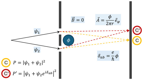
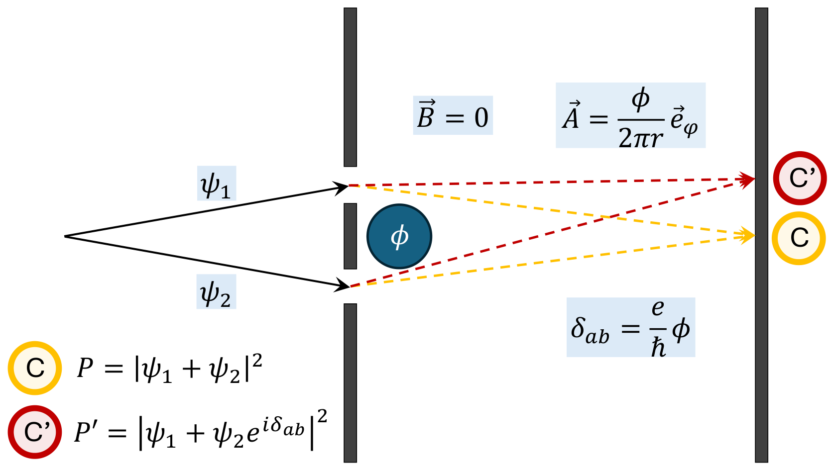
In the standard magnetic AB configuration, typically realized in a two-slit interferometric geometry, a coherent charged-particle beam is split into two components that (using a classical language) propagate along different paths and are then recombined, while a confined magnetic flux is placed between the two paths (Figure 1). In the ideal case, the magnetic field is confined within the solenoid and therefore vanishes in the region accessible to the particles, whereas the vector potential A is non-zero. As a result, the relative phase of the two wave-function components is shifted by an amount determined by the magnetic flux enclosed by the interferometer, even though no classical force acts along either path.
Figure 1.
An example of the geometry for an experiment aimed at verifying the magnetic AB effect. With respect to the no-flux case (C), the presence of the magnetic flux and the magnetic potential induces a phase shift () between the two wave functions 1 and 2. The two respective interference probabilities P and then differ by the AB phase factor .
Even before its experimental demonstration, the AB effect generated a lively debate between theoreticians and experimentalists, thoroughly described in ref. [3], and prompted several experimental investigations, culminating with the 1986 experiment of Tonomura and colleagues [4]. This clear demonstration of the effect, obtained by excluding the magnetic field from the electron classical path with the help of a superconducting film, was then supplemented by additional experiments devoted to the verification of the “zero force” condition. This verification was made through a careful study of the arrival times of the electrons in the Caprez experiment [5], with the direct demonstration that no electromagnetic forces were acting on the propagation of the particle wave-packet.
In parallel with these developments, theoretical studies highlighted the connection between the AB effect and the broader concept of geometric (Berry’s) phases in quantum mechanics [6]. The AB effect belongs to that subset of geometrical effects that are called topological, since they depend only the general topology of the system (and not on the details of the geometrical path classically followed by the particles). Moreover, in 2016 the effect was demonstrated in the original two-slit Ehrenberg–Siday configuration, as in Figure 1, by G. Pozzi and collaborators [7]; they made use of a uniformly magnetized bar with uniform cross-section, whose effect is the same as that of a straight, ideally infinite solenoid.
From an experimental point of view, in addition to the demonstration of the electric AB effect with electrons (see Appendix A), related interferometric studies have also been performed with neutrons. Since the neutron is electrically neutral, these experiments do not constitute direct realizations of the standard charge-based magnetic AB effect considered here. Rather, they involve AB-type phase phenomena associated with the neutron magnetic dipole moment, such as the Aharonov–Casher effect [8], where a magnetic moment encircles an electric charge distribution and the scalar AB analogue is produced by a pulsed magnetic field. For completeness, a brief discussion of these neutron experiments and of their conceptual distinction from the charged-particle AB effect is given in Appendix B.
Despite this extensive experimental and theoretical background, the magnetic AB effect for charged particles has so far been demonstrated for a single elementary particle of the Standard Model: the electron. It has never been studied with another charged particle, and in particular never with a composite charged hadron, such as the antiproton.
First of all, this would constitute a test of the wave-like nature of the antiproton, in addition to the well-known case of hadron scattering, low energy antiproton scattering [9] and protonium lifetime studies [10].
Secondly, such an experiment would confirm that the sign of a particle’s electromagnetic coupling does not alter the topological, field-free nature of quantum phase shifts, therefore studying in a novel way the gauge invariance for composite particles. This would be relevant for the CVC (Conserved Vector Current) concept and the Ward–Takahashi identity [11,12] describing how gauge symmetry restricts the quantum interaction of particles. The interest in interferometric studies with antiprotons is well recognized in the literature (see, e.g., Ref. [13]).
A further objective of the experiment is to investigate the dependence of the interference pattern on the direction of magnetization, and hence on the sign of the enclosed magnetic flux. A left-right asymmetry was recently observed in a high-statistics AB experiment with electrons [14], indicating a dependence on the sign of the magnetization. This effect has been suggested to originate from a breakdown of the paraxial approximation normally used in scattering theory, as proposed by Shelankov [15] and further discussed by Berry [16].
The detection of the AB effect relies on the observation of a phase-induced change in the interference pattern produced by a grating configuration. For this reason, the first step of the present study is the direct demonstration of quantum interference with antiprotons in the proposed grating configuration. This would represent the second observation of matter-wave interference with an antiparticle, after the positron interferometry experiment reported in 2019 [17], and would provide the necessary experimental basis for the subsequent measurement of the antiproton AB phase.
2. Experimental Strategy
In order to study the AB effect with the antiproton, the realization of quantum interference is a necessary precondition. Given the mass of the particle, it is important to use a low-energy beam, such as the one that is available at the CERN ASACUSA experiment. In ASACUSA, antiprotons coming from the CERN accelerator system are trapped and cooled in the MUSASHI Penning–Malmberg trap [18]. This allows the subsequent formation of a slow antiproton beam with a kinetic energy of about 250 eV.
This slow antiproton beam has already been used in another experimental study [19] and, given its low energy, has a de Broglie wavelength of
in the non-relativistic approximation. The beam has a velocity of 220,000 m/s and an intensity in the range of particles/s, for an overall spill duration of 10 s. In these conditions the total statistical accumulation will be of incoming antiprotons every 130 s, which is the repetition rate of the CERN Antiproton Decelerator, which supplies the ASACUSA setup [20].
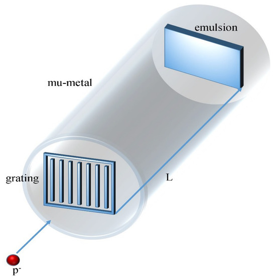
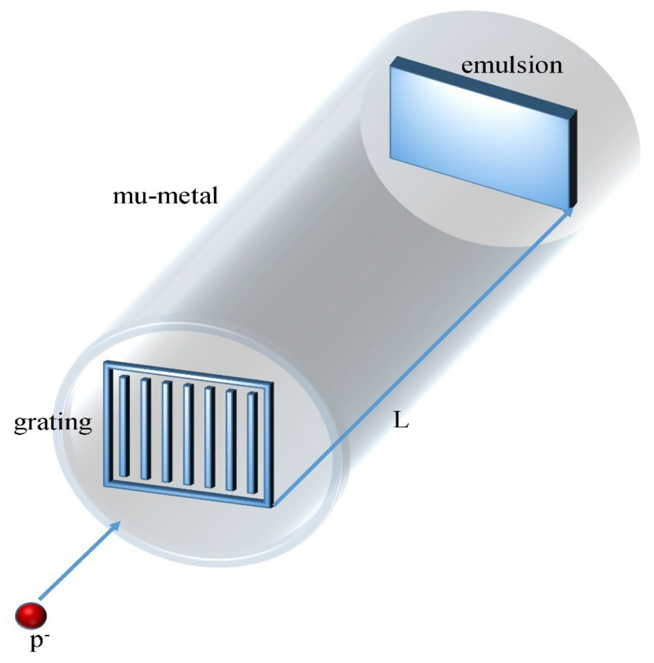
The incoming antiprotons will be studied in a 1 m long interferometer, schematically shown in Figure 2. Given the beam velocity, the transit time will be about 5 s and the mean particle arrival rate is around 100 s−1; therefore, one can safely conclude that the experiment will work in single-particle mode. This is another novelty of this approach with respect to the work done with electrons.
Figure 2.
General scheme of the AIABE setup. The grating generates a diffraction pattern to be recorded in the emulsion detector. The system is 1 m long and will be enclosed in a mu-metal shield to mitigate the effect of the Earth’s magnetic field.
Detecting with good resolution an antiproton interference pattern is a prerequisite for the demonstration of the AB effect. For this reason, as a first step, we propose a Fraunhofer diffraction experiment according to the conceptual scheme presented in Figure 2.
Given the de Broglie wavelength under consideration, a 100 nm grating structure would diffract at 18 m after a 1 m flight length. The detection therefore appears feasible with a very-high-resolution detector. For this reason, we propose the use of emulsion detectors, to be used as integrators of the diffraction signal. Emulsion films have a superior space resolution, in our case better than 1 m [21,22], and they can detect the impact point of antiprotons by reconstructing the relevant annihilation pions.
While traveling through the interferometer, the antiproton will be subjected to the Earth’s magnetic field, which requires the presence of a mu-metal shielding. The deflection of a 250 eV antiproton traveling 1 m in the Earth magnetic field is of the order of 1 cm, which is reduced to only 10 m by the kind of mu-metal used in [17]. In principle, a static magnetic field does not compromise the experiment, since it only produces an overall shift of the interference pattern. However, its space variations and fluctuations in time can be problematic. For this reason we assume a shielding factor of , as achieved with the shielding employed in [17].
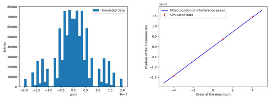
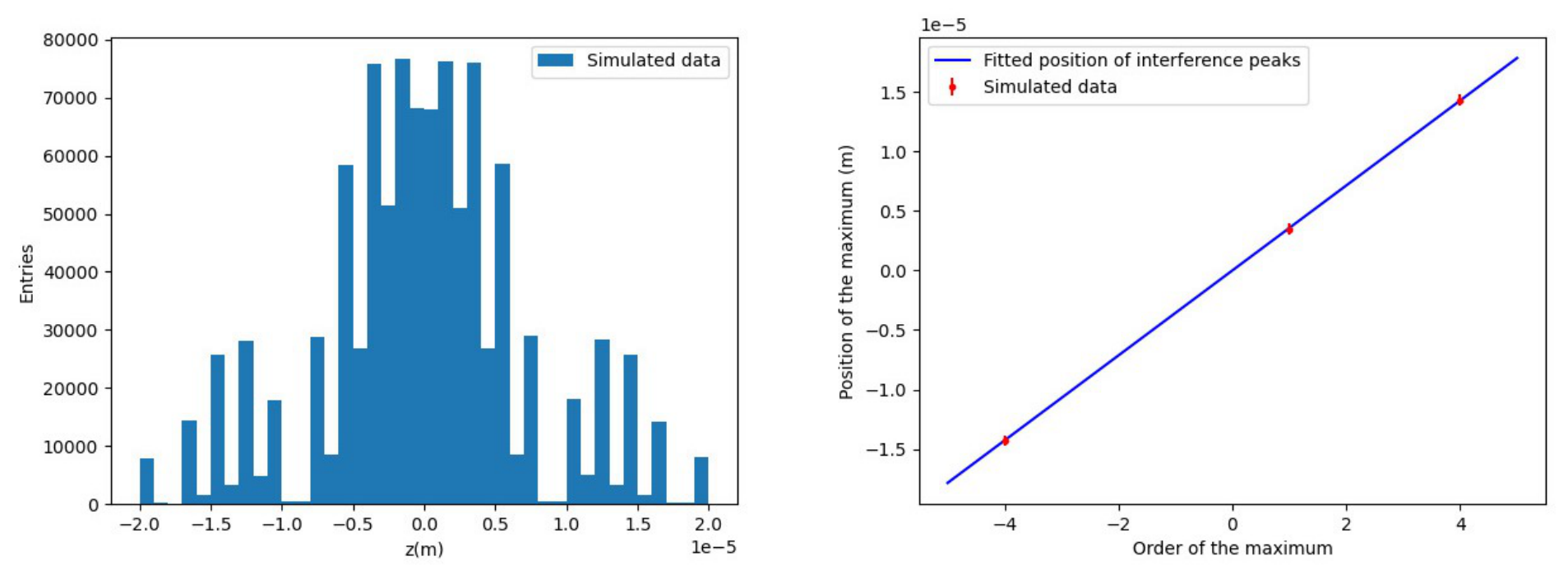
Following the scheme of Figure 2, a first direct demonstration of antiproton interferometry can be obtained by a Fraunhofer interference–diffraction experiment with material grating. In order to substantiate this idea, a simulation was made assuming a material grating with slits, each having an aperture of 200 nm and an inter-slit distance of 10 m. A 250 eV antiproton beam impinging on the grating would produce an interference pattern on the emulsion (after 1 m flight path), such as the one shown in Figure 3 (left). The simulation assumes 106 detected particles and includes effects of energy and space resolution of the emulsion.
Figure 3.
Simulation of the effect of a 250 eV antiproton beam of 106 particles and a grating with slits, each having a 200 nm aperture and with an inter-slit distance of 10 m. (Left) Distribution of the impact points on the detector after 1 m flight path following the grating. (Right) Three points of the impact distribution are fit to the theoretical curve to obtain the de Broglie wavelength. The simulation includes effects such as energy and detector resolution.
Given the geometric configuration, and the open fraction of the grating (about 2%), an amount of impinging antiprotons is necessary to produce the pattern in the figure, which is achievable with 3–4 days of data taking at the Antiproton Decelerator.
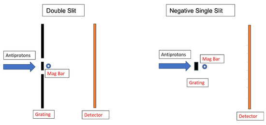
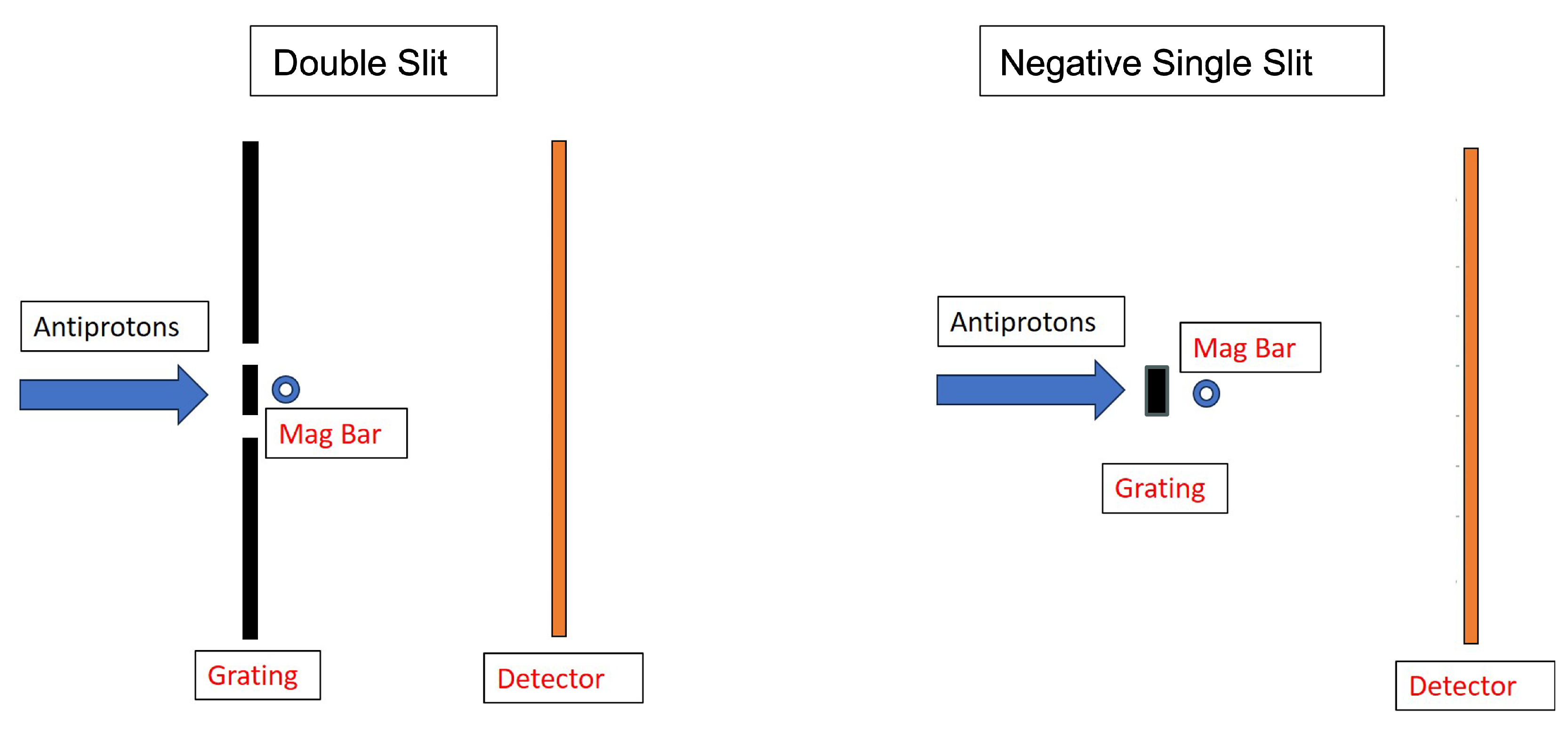
Once antiproton interferometry has been demonstrated, the next logical step is the demonstration of the AB effect. This will be achieved following the conceptual scheme presented in Figure 4, where the classical double slit configuration as well as an anti-configuration (small obstacle instead of a grating with slits) are shown.
Figure 4.
The configurations for the AB experiment. On the left hand side the classical Young style configuration is shown. In our experiment we will instead use configurations of the type shown on the right, with a “negative” single obstacle configuration giving the same interferometric result of a single slit diffraction setup (Babinet principle) and allowing a much higher antiproton flux to reach the detector.
To properly simulate the AB effect in our proposed configuration, we have modeled the wave mechanical free-space propagation of the antiproton wavefront from the (anti)slit(s) by solving analytically the Fresnel–Kirchhoff integral in the paraxial approximation all the way from Fresnel to Fraunhofer, following the standard image formation scheme universally adopted in optics [23].
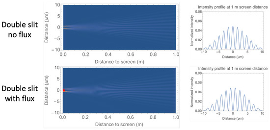
Under these conditions, the interference–diffraction of the 250 eV antiprotons would produce a theoretical pattern on the detector, as shown in Figure 5, where the difference between the two cases consists in a single unit of magnetic flux. The pattern of the minima and maxima are within the range of sensitivity of the emulsion detector even after 50 cm of propagation.
Figure 5.
The interference and diffraction system generated by a two slit system under the condition on the left-side of Figure 4, opening 500 nm, inter-slit distance 1 m and 1 m distance from the detector/screen. The difference is of a single unit of magnetic flux (red dot).
In a configuration like this, let us consider the following (realistic) parameters:
- Slit opening nm;
- Inter-slit distance m for the double slit case;
- Grating-detector distance of 1 m.
The working principle of the emulsion detector is based on the measurement of the antiproton impact point (see Figure 5) through the reconstruction of the annihilation tracks produced by the outgoing pions. This technique relies on tracing, within the emulsion, the tracks produced by the annihilation of the antiproton. The 2–3 pions typically produced leave distinct tracks that can be reconstructed as discussed in [21,22]. According to this reconstruction technique, the expected uncertainty in the reconstructed antiproton impact position is about one micron.
However, the use of a classical two-slit configuration with material gratings has the significant disadvantage of reducing the incoming antiproton flux. In addition, antiprotons stopped by materials generate pions, and that background can be important.
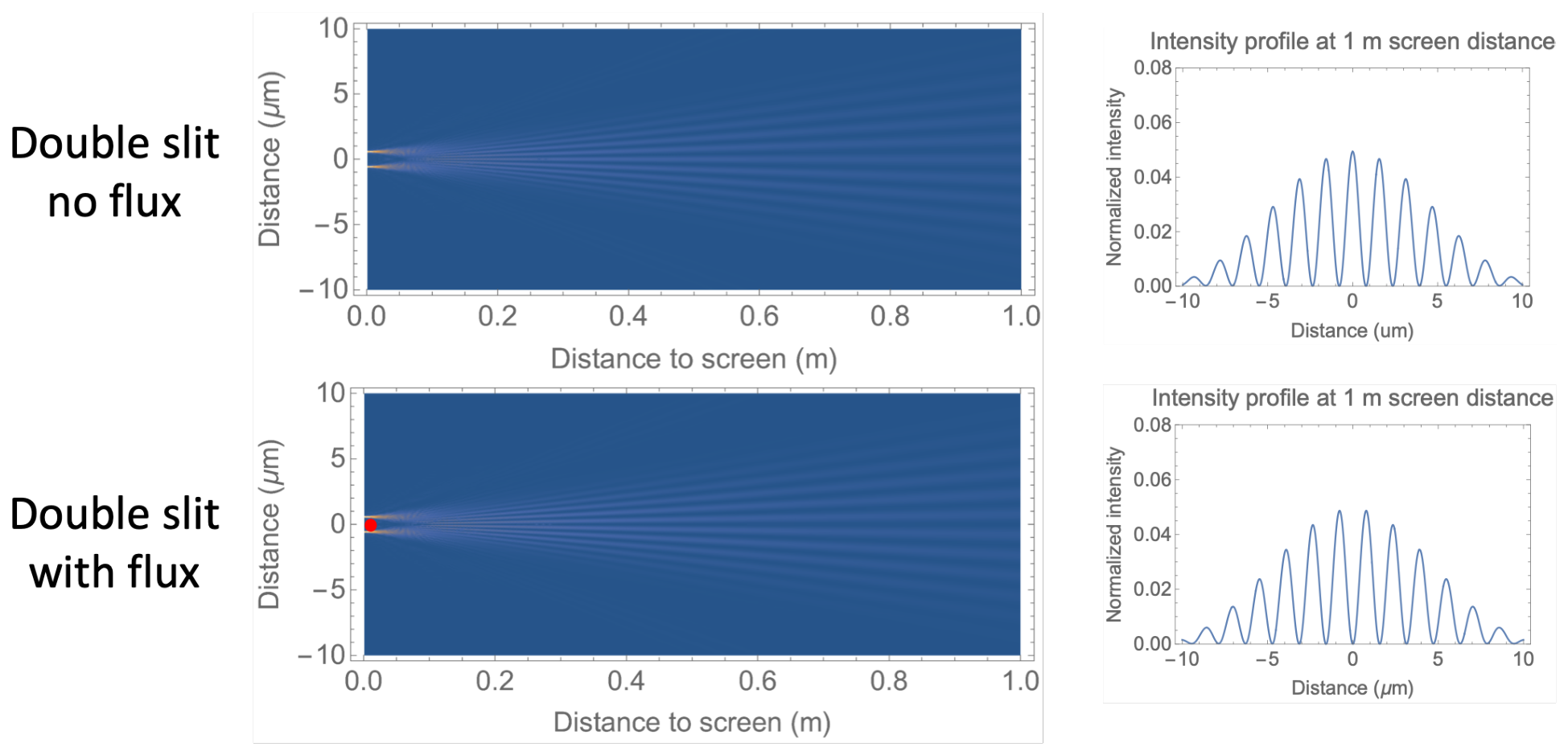
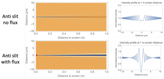
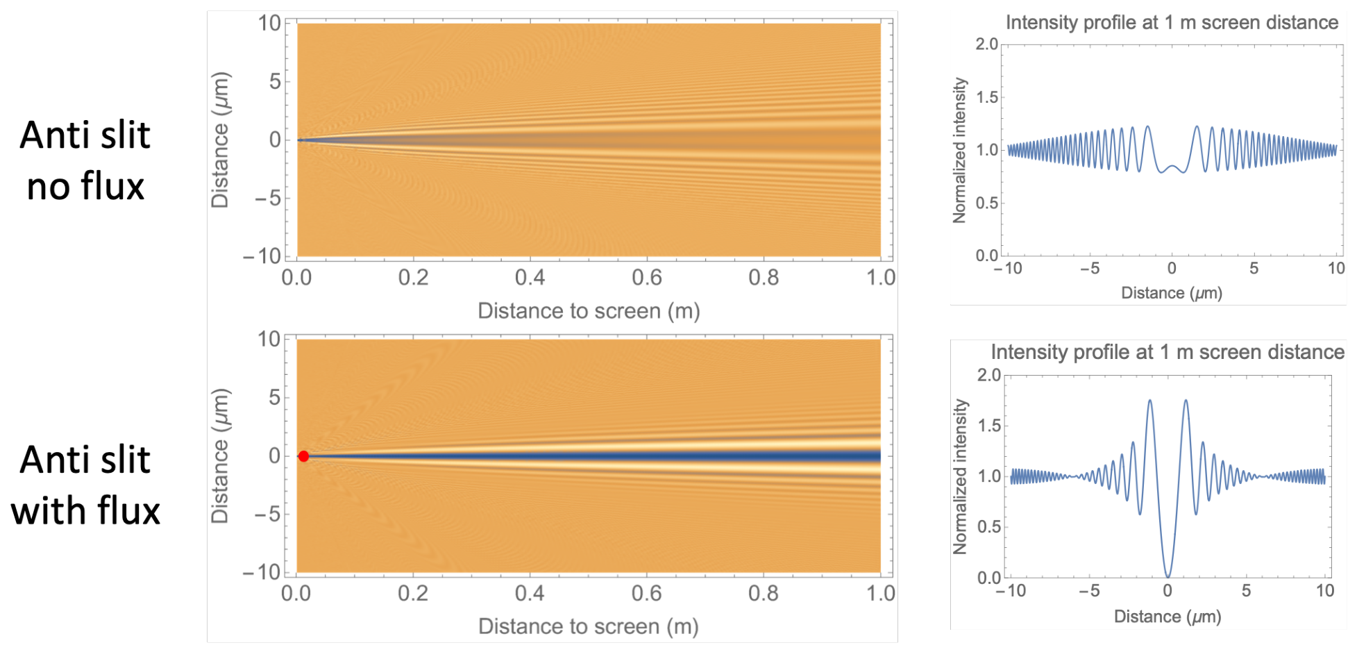
In order to overcome these problems, we will use a configuration like the one shown on the right-hand side of Figure 4. The interferometric result of a configuration of this type is shown in the lower part of Figure 6. By contrast, the upper part of Figure 6 illustrates the case with no magnetic flux present.
Figure 6.
The configurations for the AB experiment would produce an interference and diffraction pattern indicated in the figure, after propagation to the detector. The upper part refers to the presence of the obstacle alone (150 nm wide), while the lower part includes the magnetized bar generating one unit of magnetic flux (red dot).
As the magnetic element, we will use the bars developed for the AB experiment with electrons, as in [7,24]. Therefore, we propose a configuration like the one outlined in the right part of Figure 4, producing the interference pattern displayed in Figure 6.
The study of the magnetic AB effect will be conducted by varying the angle of inclination of the magnetized bar, so that the amount of magnetic flux enclosed by the path of the particles can be varied continuously.
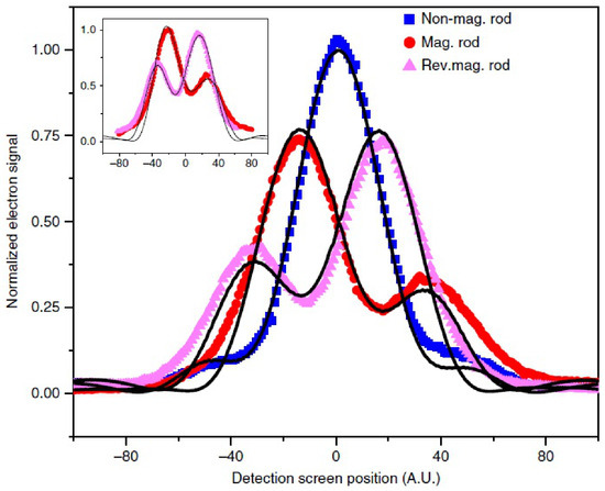
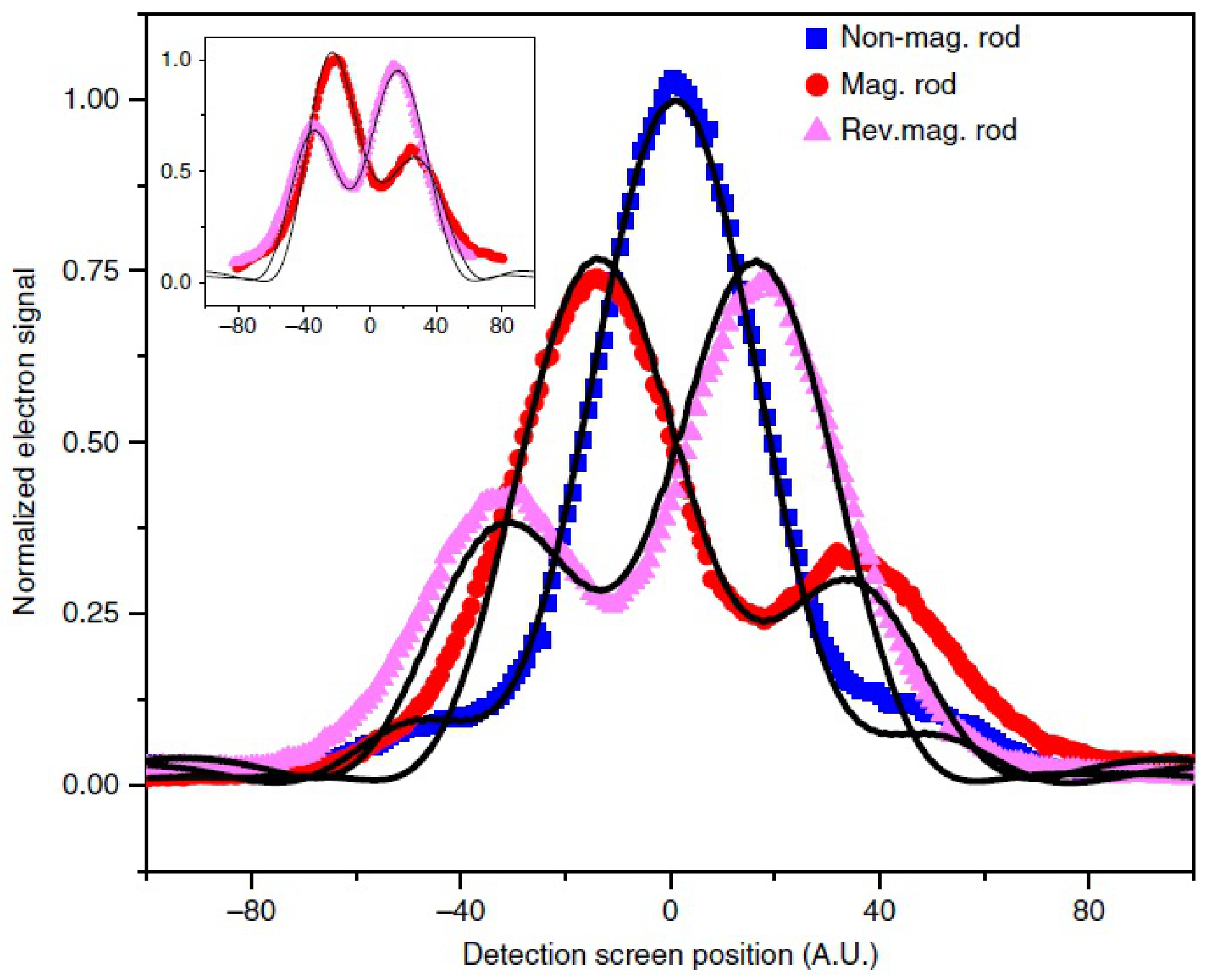
The specific signature of the AB effect will be the asymmetry between the two cases of currents described in [14] and shown in Figure 7, corresponding to a rotation of the magnetic bar by 180 degrees. In addition, all the intermediate rotation angles will be available, including 90 degrees, which produces the case of zero magnetic flux and provides a normalization of the effect.
Figure 7.
Symmetry reversal of the AB effect with electrons from the experiment in [14] with electrons. The electron beam was impinging on a single magnetized rod and the AB effect shown here refers to two different signs obtained by rotating the magnetic rod by 180 degrees. The inset contains only the two configurations with the magnetic rod, while the figure also shows for comparison the blank (no-rod) configuration. Figure from ref. [14], reprinted with permission from the author.
3. Conclusions
We propose the exploration of antiproton interferometry in conjunction with the AB effect, by making use of the slow antiproton beam available at the ASACUSA setup in the CERN Antiproton Decelerator.
The experiment, divided into a first demonstration of antiproton interferometry and a following demonstration of the AB effect, is intended to study this quantum–mechanical phenomenon with a non-elementary antiparticle.
Author Contributions
Conceptualization, A.A., M.N.B., F.C., G.D.L., V.T. (Valeri Tioukov) and L.V.; methodology, T.A., M.B., N.D., R.F., S.M. (Stefano Migliorati) and T.N.; software, G.R.; resources, S.F., A.G., G.C.G., V.G., M.L., V.M., S.M. (Simone Masci) and V.T. (Valerio Toso); writing—original draft, M.G.; writing—review and editing, M.G., G.M., F.M. and M.R. Author Fabrizio Castelli passed away prior to the publication of this manuscript. All other authors have read and agreed to the published version of this manuscript.
Funding
This research received no external funding.
Data Availability Statement
The raw data supporting the conclusions of this article will be made available by the authors on request.
Acknowledgments
We would like to thank the ASACUSA Collaboration for considering the possibility of conducting this experiment in the frame of their experimental apparatus at CERN. This paper is dedicated to the memory of our colleague and co-author Fabrizio Castelli, who passed away during the preparation of this work. Finally, we also thank Herman Batelaan for the useful discussions.
Conflicts of Interest
The authors declare no conflicts of interest.
Appendix A. The Aharonov-Bohm Effect
The Aharonov–Bohm effect refers to the quantum-mechanical situation that arises when particles pass through regions where the potentials and A are nonzero, whereas the physical fields (electric field E and magnetic field B) are zero and therefore no force is present in the classical sense.
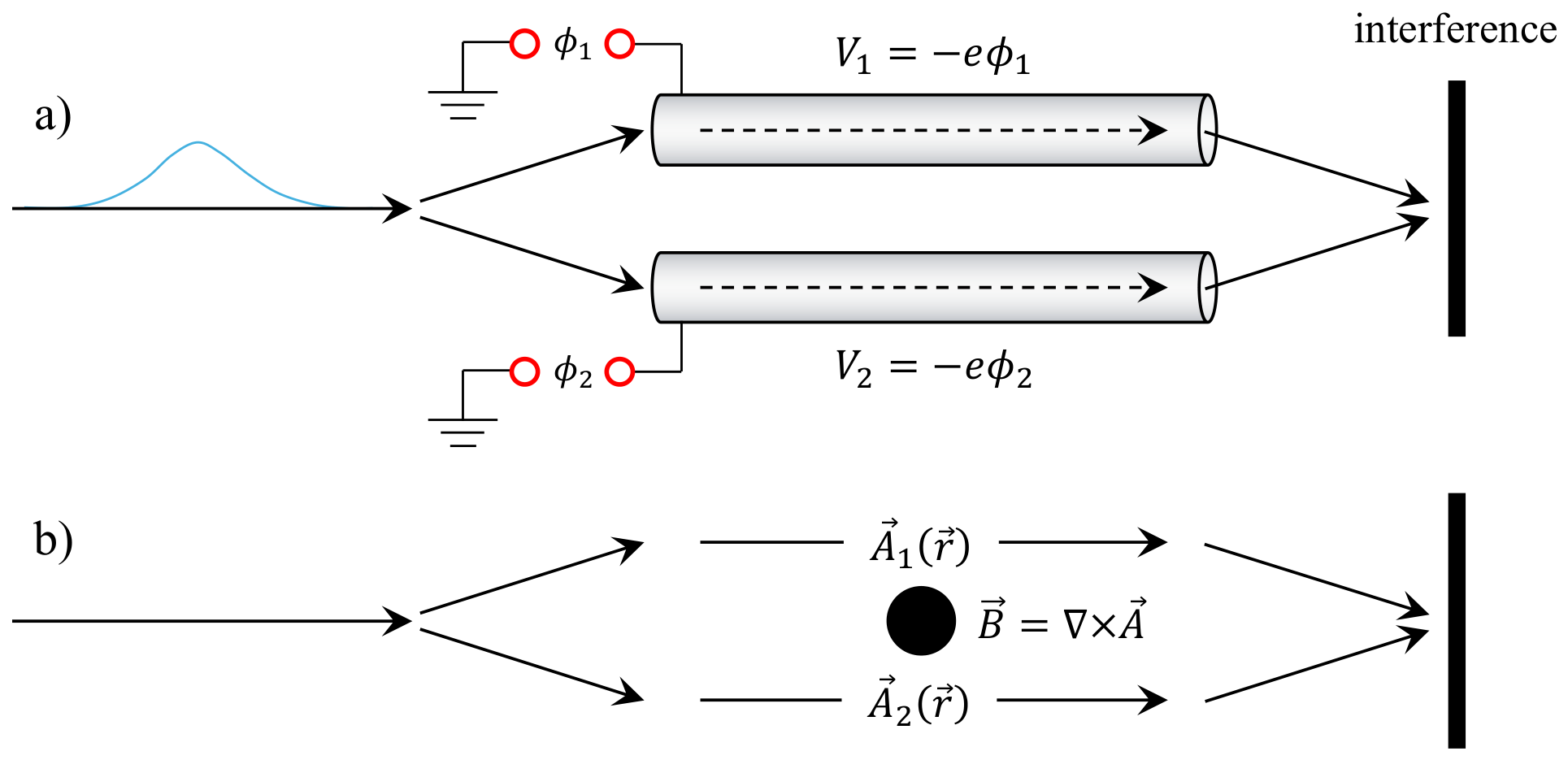
For a charged particle, the wave function describing its dynamics can be expressed in such a way that the electromagnetic potentials and A appear in its phase. For example, an electron wave packet traveling in a region of potential energy , acquires a phase . This follows directly from the Hamiltonian, which in this case is . The AB effect in this case is shown in Figure A1a, where the wavefunction is split into two wave packets that (in the classical sense) will follow two different paths within two different conducting cylinders.
When the electron wave packets are inside the cylinders, one can turn on the potentials and , which are switched off just before they leave the cylinders. The packets now have acquired a phase which is and ( being the crossing time of the cylinders). These two phases differ if . Now note that the electric field E acting on the packet classical path is always zero. Then, instead of experiencing E directly (and therefore a force), the particle is only subjected to the potential associated to E. The difference in the electrostatic potential of course has physical effects when the two wave packets are recombined; these effects were observed for the first time (demonstration of the electric AB effect) only in 1998 [25].
The situation in Figure A1b is similar in spirit but concerns the most common case of the magnetic AB effect. We split the wave packet into two separate wave packets, then let them pass in a region where there is a solenoid. Since the field is confined inside the solenoid, while .
It is noteworthy that quantum mechanical waves are sensitive to potentials, which are not gauge-invariant quantities. Consider the gauge transformation , where is an arbitrary function of space and time. The wavefunction must change accordingly so that the transformation has no physical effect. This is one of the features that distinguishes classical particles from quantum particles.
Figure A1.
(a) Schematic representation of the so-called electric Aharonov–Bohm effect. After the wave packet has been split, the two parts pass in the region where and are different from zero. The electric field E is zero inside the cylinders (but not everywhere). (b) Schematic representation of the magnetic Aharonov–Bohm effect; again we split the wave packet in two and then we let it pass in a region where A is nonzero while B = 0 due to the presence of an ideal solenoid. The only part where the magnetic field is nonzero is inside the solenoid.
In regions where , to obtain the effect brought by we only need to calculate a phase by integrating over a convenient path. Consider the time-dependent Schrödinger equation for a particle with charge q in a region where , such as a path around the solenoid
The solution to this equation is given by the solution times a phase factor
In fact, inserting the solution in (A1) one has
This shows that the effect on the wave function caused by in a region where is accounted for by a phase factor.
The typical geometry for an experiment on the magnetic AB effect is the one shown in part b) of Figure A1. The field (pointing outside of the page) is present only in the region inside the solenoid, while outside the cylinder , so particles experience but not . In the region where , where a is the radius of the solenoid, we have
where points counterclockwise. Then, at the point of closest approach, the “lower” component of points in the same direction of momentum of the wave packet, while the “upper” part points in the opposite direction; so phase shifts are introduced for both wave packets: in one case it advances the phase, in the other case it delays the phase.
Since the interference pattern depends on the phase, when we recombine the two packets we will see an effect due to the solenoid. We interpret this by saying that the vector potential has a physical effect on the system. In fact, the presence of results in a phase difference
We can reverse the limit of the second integral to obtain
By using Stokes’ theorem we see that the phase difference depends on the magnetic flux
with the quantum of magnetic flux.
Appendix B. Neutron Interferometry and AB-Type Phase Effects
It is appropriate to briefly recall the main results obtained in the search for AB–type effects using neutrons. Since the neutron is electrically neutral, the standard magnetic and electric AB effects discussed in Appendix A are not directly applicable. However, the neutron possesses an intrinsic magnetic dipole moment associated with its spin 1/2. This enables the occurrence of closely related quantum phase phenomena, which have been extensively investigated by neutron interferometry experiments [26]. In 1981, the group of Greenberger performed a neutron interferometry experiment explicitly designed to test the magnetic AB configuration with a solenoid, analogous to that used for charged particles [27]. No measurable phase shift was observed. The experiment set an upper bound showing that any AB phase for the neutron is smaller than about of that for a particle with charge e. This result provided a stringent experimental confirmation that the magnetic AB effect is intrinsically linked to electric charge, and simultaneously constrained the possible electric charge of the neutron to extremely small values.
In 1984, Aharonov and Casher predicted that a neutral particle carrying a magnetic dipole moment should acquire a quantum phase when moving around a distribution of electric charge [8]. In this configuration, a neutron encircling a charged wire experiences no net classical force, yet its wave function acquires a non-dispersive phase
which ultimately depends only on the total charge enclosed by the trajectory, in close analogy with the magnetic AB effect for charged particles.
However, it is worth emphasizing an important conceptual difference. In the laboratory frame, the Aharonov–Casher (AC) phase can be interpreted as a geometric or topological effect. In the neutron rest frame, however, the electric field is transformed into an effective magnetic field that couples locally to the neutron magnetic moment, leading to a spin-dependent dynamical phase. The accumulated phase can therefore be viewed as arising from the integral of this local interaction along the path. This contrasts with the magnetic AB effect for charged particles, where the AB phase arises in the absence of any local gauge-invariant interaction term in the region accessible to the particle.
The first experimental verification of the AC effect was achieved in 1989 by Cimmino et al. using a neutron interferometer, observing a phase shift in quantitative agreement with the theoretical prediction [28].
A further development concerned the analogue of the electric (or scalar) AB effect for neutrons. Although neutrons are neutral, their magnetic moment implies a magnetic potential energy . A neutron with spin parallel to a uniform static magnetic field undergoes a constant energy shift and, when traversing such a region, accumulates a phase without experiencing deflection or spin precession, in close analogy with an electron propagating in a region of constant electric potential.
In an interferometric configuration where a short magnetic-field pulse was applied synchronously to only one arm of the interferometer, a relative phase shift was observed in 1992 by Allman et al. [29], consistent with
That experiment employed an unpolarized neutron beam, consisting of two sub-populations with opposite spin orientation. Peshkin subsequently pointed out that, in this situation, the observed phase shift could in principle be interpreted as arising from the local interaction of the magnetic dipole with the time-dependent magnetic field (i.e., an ordinary Zeeman coupling), without the need to invoke a genuine AB-type mechanism [30].
A few years later the experiment was repeated by Lee et al. using a polarized neutron beam and an optimized setup [31]. In this case the scalar AB phase was observed in agreement with the predicted phase shift, exhibiting the expected linear dependence on the time integral of the magnetic field.
In summary, for neutrons both the Aharonov–Casher effect and the scalar AB analogue have been experimentally observed, whereas the standard magnetic AB effect is absent to very high precision. Unlike the case of charged particles, however, the physical interpretation of these neutron-induced phase shifts remains the subject of ongoing debate. Several authors emphasize that they can be entirely reduced to locally acting interactions between the neutron magnetic dipole moment and electromagnetic fields (in an appropriate reference frame), and therefore do not constitute a genuinely new topological effect [32]. Others, by contrast, stress that the observed phase shifts are coherent, non-dispersive quantum phenomena involving no net work performed on the particle, and thus share the defining characteristics of Aharonov–Bohm–type effects [33].
Neutron interferometry therefore provides a useful comparison, but it should not be regarded as a direct analogue of the standard magnetic AB effect for a charged particle. This distinction further highlights the interest of testing the charge-based magnetic AB phase with a massive, composite, charged antiparticle such as the antiproton, as proposed in the present work.
Appendix C. More on the Physical Meaning of the AB Effect
As we have seen, the AB effect can be interpreted as the interaction with a potential (and not a classical field), indicating that the potentials have a more fundamental role in quantum physics. And of course while the value of in the magnetic AB effect is gauge-dependent, the line-integral (the phase shift) is a gauge-invariant physical reality that affects the downstream interference pattern.
As outlined in [26], a genuine effect of the AB type must have the typical signature of being independent from the particle velocity (kinetic energy). In fact, if the AB phase shift depended on the energy, the different components of the wave packet (having different velocities) would be affected in different ways, thereby deforming (or delaying) the wave packet-which is the typical action of a force. In fact the phase shift is independent of the energy or velocity of the particle, as was also demonstrated experimentally by Caprez [5].
This distinction between shift of the phase (without force) and shift of the wave packet (with an acting force) is the key difference between topological and dynamical effect in quantum physics.
References
- Ehrenberg, W.; Siday, R.E. The Refractive Index in Electron Optics and the Principles of Dynamics. Proc. Phys. Soc. B 1949, 62, 8. [Google Scholar] [CrossRef] [Scilit]
- Aharonov, Y.; Bohm, D. Significance of Electromagnetic Potentials in the Quantum Theory. Phys. Rev. 1959, 115, 485. [Google Scholar] [CrossRef] [Scilit]
- Olariu, S.; Popescu, I.I. The quantum effects of electromagnetic fluxes. Rev. Mod. Phys. 1985, 57, 339. [Google Scholar] [CrossRef] [Scilit]
- Tonomura, A.; Osakabe, N.; Matsuda, T.; Kawasaki, T.; Endo, J. Evidence for Aharonov-Bohm effect with magnetic field completely shielded from electron wave. Phys. Rev. Lett. 1986, 56, 792. [Google Scholar] [CrossRef] [Scilit] [PubMed]
- Caprez, A.; Barwick, B.; Batelaan, H. Macroscopic Test of the Aharonov-Bohm effect. Phys. Rev. Lett. 2007, 99, 210401. [Google Scholar] [CrossRef] [Scilit] [PubMed]
- Berry, M.V. Quantal Phase Factors Accompanying Adiabatic Changes. Proc. R. Soc. Lond. Ser. 1984, A 392, 45. [Google Scholar] [CrossRef] [Scilit]
- Pozzi, G.; Boothroyd, C.B.; Tavabi, A.H.; Yücelen, E.; Dunin-Borkowski, R.E.; Frabboni, S.; Gazzadi, G.C. Experimental realization of the Ehrenberg-Siday thought experiment. Appl. Phys. Lett. 2016, 108, 083108. [Google Scholar] [CrossRef] [Scilit]
- Aharonov, Y.; Casher, A. Topological Quantum Effects for Neutral Particles. Phys. Rev. Lett. 1984, 53, 319–321. [Google Scholar] [CrossRef] [Scilit]
- Knudsen, H.; Kristiansen, H.-P.E.; Thomsen, H.D.; Uggerhøj, U.I.; Ichioka, T.; Møller, S.P.; Hunniford, C.A.; McCullough, R.W.; Charlton, M.; Kuroda, N.; et al. Ionization of Helium and Argon by Very Slow Antiproton Impact. Phys. Rev. Lett. 2008, 101, 043201. [Google Scholar] [CrossRef] [Scilit] [PubMed]
- Amsler, C. Proton-antiproton annihilation and meson spectroscopy with the Crystal Barrel. Rev. Mod. Phys. 1998, 70, 1293. [Google Scholar] [CrossRef] [Scilit]
- Ward, J.C. An Identity in Quantum Electrodynamics. Phys. Rev. 1950, 78, 182. [Google Scholar] [CrossRef] [Scilit]
- Takahashi, Y. On the generalized Ward Identify. Il Nuovo Cim. 1957, 6, 371. [Google Scholar] [CrossRef] [Scilit]
- Müller, S.R.; Nedelec, P.; Oberthaler, M.K. From classical xenon fringes to hydrogen interferometry. New J. Phys. 2020, 22, 073060. [Google Scholar] [CrossRef] [Scilit]
- Becker, M.; Guzzinati, G.; Béché, A.; Verbeeck, J.; Batelaan, H. Asymmetry and non-dispersivity in the Aharonov-Bohm effect. Nat. Comm. 2019, 10, 1700. [Google Scholar] [CrossRef] [Scilit] [PubMed]
- Shelankov, A.L. Magnetic force exerted by the Aharonov-Bohm line. Europhys. Lett. 1998, 43, 623. [Google Scholar] [CrossRef] [Scilit]
- Berry, M.V. Aharonov-Bohm beam deflection: Shelankov’s formula, exact solution, asymptotics and an optical analogue. J. Phys. A Math. Gen. 1999, 32, 5627. [Google Scholar] [CrossRef] [Scilit]
- Sala, S.; Ariga, A.; Ereditato, A.; Ferragut, R.; Giammarchi, M.; Leone, M.; Pistillo, C.; Scampoli, P. First demonstration of antimatter wave interferometry. Sci. Adv. 2019, 5, eaav7610. [Google Scholar] [CrossRef] [Scilit] [PubMed]
- Kuroda, N.; Torii, H.A.; Nagata, Y.; Shibata, M.; Enomoto, Y.; Imao, H.; Kanai, Y.; Hori, M.; Saitoh, H.; Higaki, H.; et al. Development of a monoenergetic ultraslow antiproton beam source for high-precision investigation. Phys. Rev. Spec. Top. 2012, 15, 024702. [Google Scholar] [CrossRef] [Scilit]
- Amsler, C.; Breuker, H.; Bumbar, M.; Cerwenka, M.; Costantini, G.; Ferragut, R.; Fleck, M.; Giammarchi, M.; Gligorova, A.; Gosta, G.; et al. Antiproton annihilation at rest in thin solid targets and comparison with Monte Carlo simulations. Eur. Phys. J. A 2024, 60, 225. [Google Scholar] [CrossRef] [Scilit] [PubMed]
- Hunter, E.D.; Bumbar, M.; Amsler, C.; Bayo, M.; Breuker, H.; Cerwenka, M.; Costantini, G.; Ferragut, R.; Giammarchi, M.; Gligorova, A.; et al. Optimizing antihydrogen production via slow plasma merging. Phys. Plasmas 2026, 33, 032119. [Google Scholar] [CrossRef] [Scilit]
- Ariga, A.; Ariga, T.; De Lellis, G.; Ereditato, A.; Niwa, K. Nuclear Emulsions. In Particle Physics Reference Library; Fabjan, C., Schopper, H., Eds.; Springer: Cham, Switzerland, 2020. [Google Scholar] [CrossRef] [Scilit]
- Alexandrov, A.; Buonaura, A.; Consiglio, L.; D’Ambrosio, N.; De Lellis, G.; Di Crescenzo, A.; Galati, G.; Lauria, A.; Montesi, M.C.; Tioukov, V.; et al. A new generation scanning system for the high-speed analysis of nuclear emulsions. J. Instrum. 2016, 11, P06002. [Google Scholar] [CrossRef] [Scilit]
- Born, M.; Wolf, E. Principle of Optics, 6th ed.; Pergamon Press: Oxford, UK, 1980. [Google Scholar]
- Gazzadi, G.C.; Mulders, H.; Trompenaars, P.; Ghirri, A.; Affronte, M.; Grillo, V.; Frabboni, S. Focused electron beam deposition of nanowires from cobalt tricarbonyl nitrosyl (Co(Co)3NO) precursor. J. Phys. Chem. C 2011, 115, 19606. [Google Scholar] [CrossRef] [Scilit]
- van Oudenaarden, A.; Devoret, M.H.; Nazarov, Y.V.; Mooij, J.E. Magneto-electric Aharonov–Bohm effect in metal rings. Nature 1998, 391, 768. [Google Scholar] [CrossRef] [Scilit]
- Zeilinger, A. Generalized Aharonov-Bohm Experiments with Neutrons. In Fundamental Aspects of Quantum Theory; NATO ASI Series; Springer: Boston, MA, USA, 1986; Volume 144, p. 311. [Google Scholar] [CrossRef] [Scilit]
- Greenberger, D.M.; Atwood, D.K.; Arthur, J.; Shull, C.G.; Schlenker, M. Is There an Aharonov-Bohm Effect for Neutrons? Phys. Rev. Lett. 1981, 47, 751–754. [Google Scholar] [CrossRef] [Scilit]
- Cimmino, A.; Opat, G.I.; Klein, A.G.; Kaiser, H.; Werner, S.A.; Arif, M.; Clothier, R. Observation of the topological Aharonov–Casher phase shift by neutron interferometry. Phys. Rev. Lett. 1989, 63, 380–383. [Google Scholar] [CrossRef] [Scilit] [PubMed]
- Allman, B.E.; Cimmino, A.; Klein, A.G.; Opat, G.I.; Kaiser, H.; Werner, S.A. Scalar Aharonov–Bohm experiment with neutrons. Phys. Rev. Lett. 1992, 68, 2409–2412. [Google Scholar] [CrossRef] [Scilit] [PubMed]
- Peshkin, M. Comment on “Scalar Aharonov–Bohm experiment with neutrons”. Phys. Rev. Lett. 1992, 69, 2017. [Google Scholar] [CrossRef] [Scilit] [PubMed]
- Lee, W.-T.; Motrunich, O.; Allman, B.E.; Werner, S.A. Observation of Scalar Aharonov–Bohm Effect with Longitudinally Polarized Neutrons. Phys. Rev. Lett. 1998, 80, 3165–3168. [Google Scholar] [CrossRef] [Scilit]
- Peshkin, M.; Lipkin, H.J. Topology, Locality, and Aharonov-Bohm Effect with Neutrons. Phys. Rev. Lett. 1995, 74, 2847–2850. [Google Scholar] [CrossRef] [Scilit] [PubMed]
- Cimmino, A.; Allman, B.E.; Klein, A.G.; Kaiser, H.; Werner, S.A. High precision measurement of the topological Aharonov–Casher effect with neutrons. Nucl. Instrum. Methods Phys. Res. A 2000, 440, 579–584. [Google Scholar] [CrossRef] [Scilit]
Disclaimer/Publisher’s Note: The statements, opinions and data contained in all publications are solely those of the individual author(s) and contributor(s) and not of MDPI and/or the editor(s). MDPI and/or the editor(s) disclaim responsibility for any injury to people or property resulting from any ideas, methods, instructions or products referred to in the content. |
© 2026 by the authors. Licensee MDPI, Basel, Switzerland. This article is an open access article distributed under the terms and conditions of the Creative Commons Attribution (CC BY) license.