Figure 1.
The
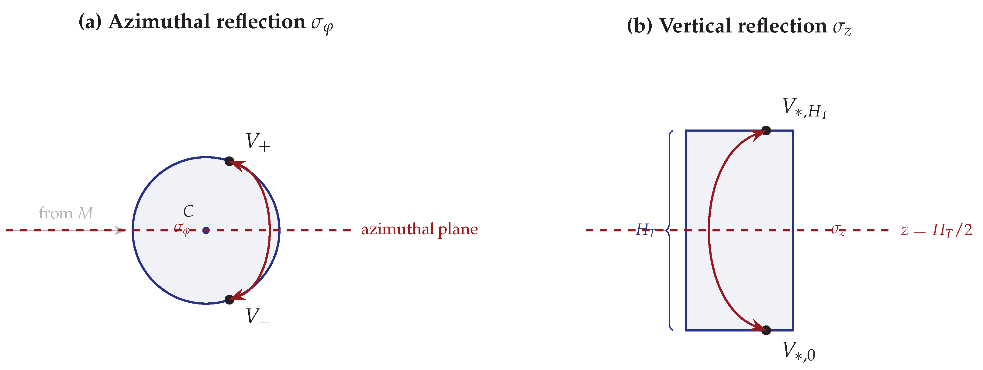
mirror symmetry group acting on the cylindrical silhouette. (
a) The azimuthal reflection
across the vertical plane containing the missile–target bearing exchanges the two tangent points
. (
b) The vertical reflection
across the cylinder’s mid-height plane exchanges the top and bottom endpoints. Because
and
commute and each is of order two, they generate a group isomorphic to the Klein four-group
, whose four-element orbit is precisely
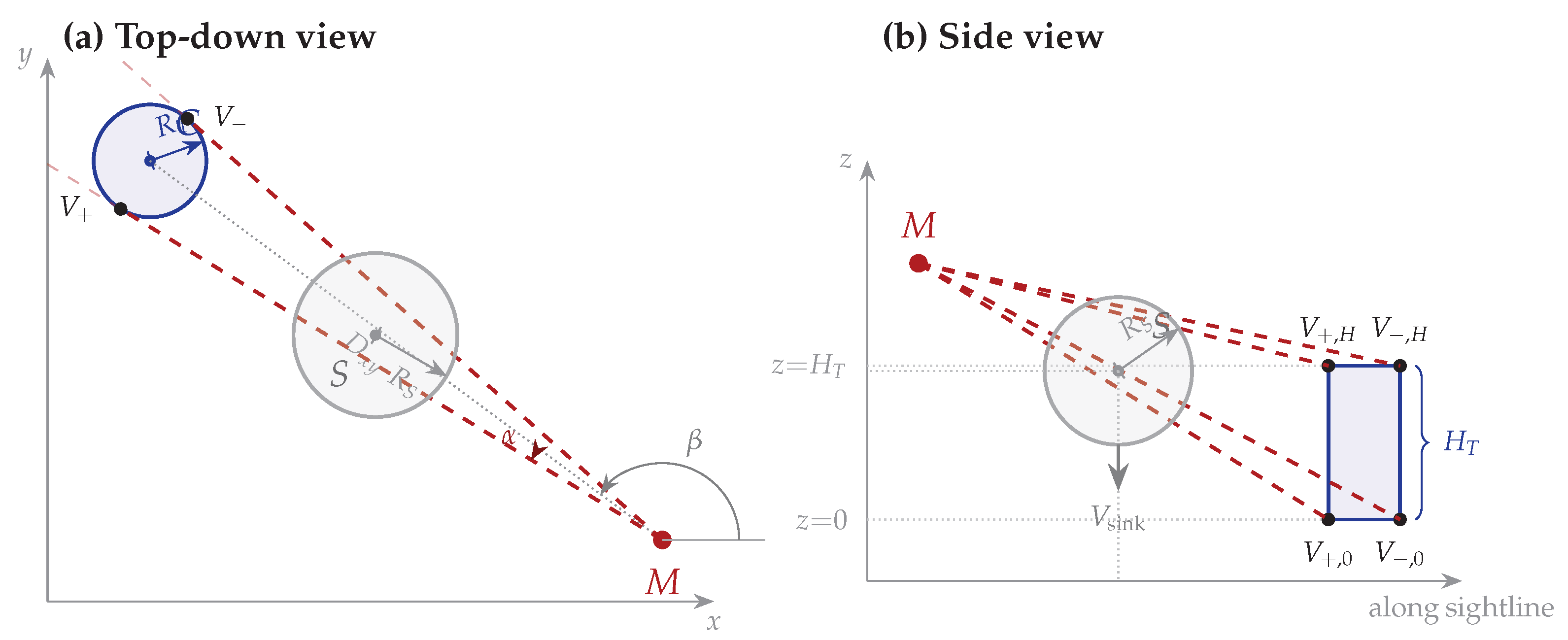
. These four points are precisely the extreme sightline targets that will be formally introduced in
Section 2.4 as Equation (
8).
Figure 1.
The
mirror symmetry group acting on the cylindrical silhouette. (
a) The azimuthal reflection
across the vertical plane containing the missile–target bearing exchanges the two tangent points
. (
b) The vertical reflection
across the cylinder’s mid-height plane exchanges the top and bottom endpoints. Because
and
commute and each is of order two, they generate a group isomorphic to the Klein four-group
, whose four-element orbit is precisely
. These four points are precisely the extreme sightline targets that will be formally introduced in
Section 2.4 as Equation (
8).
Figure 2.
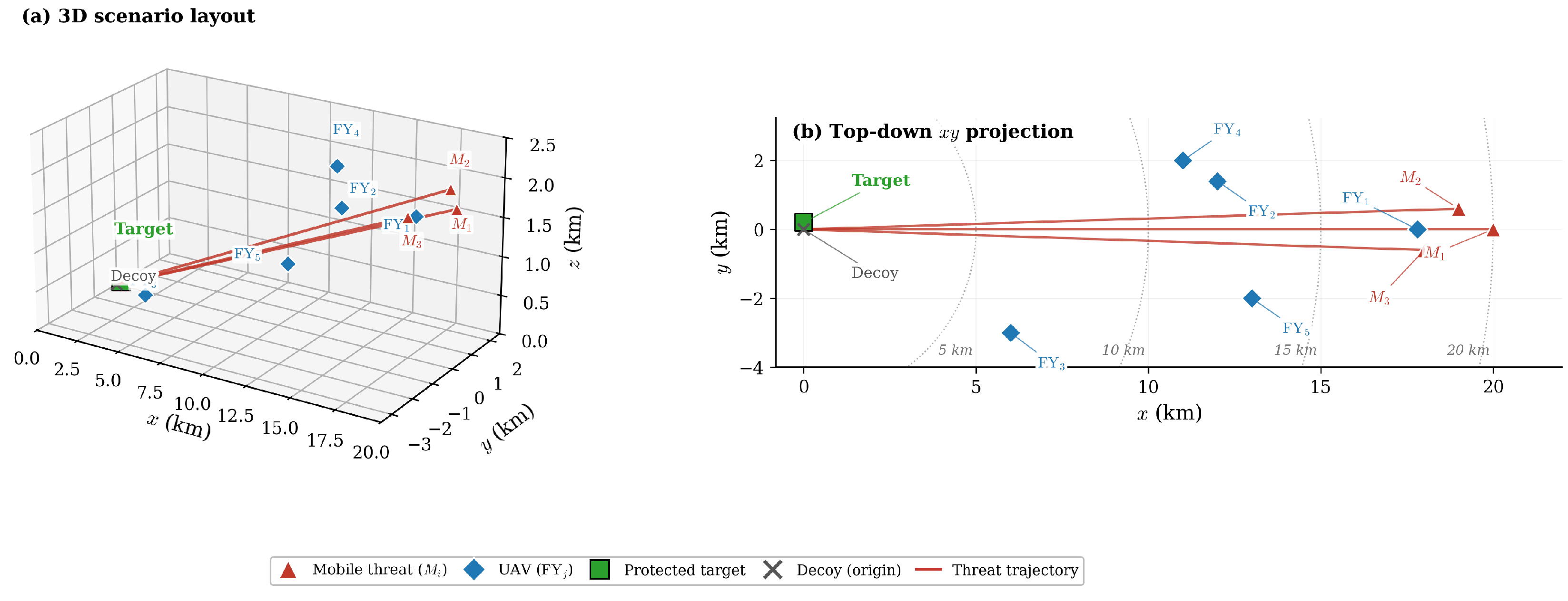
Scenario layout. (a) Three-dimensional view showing missile trajectories (red), UAV initial positions (diamonds), the defended vessel (green square at m), and the decoy at the origin. (b) Top-down -plane projection with range rings indicating distance from the decoy.
Figure 2.
Scenario layout. (a) Three-dimensional view showing missile trajectories (red), UAV initial positions (diamonds), the defended vessel (green square at m), and the decoy at the origin. (b) Top-down -plane projection with range rings indicating distance from the decoy.
Figure 4.
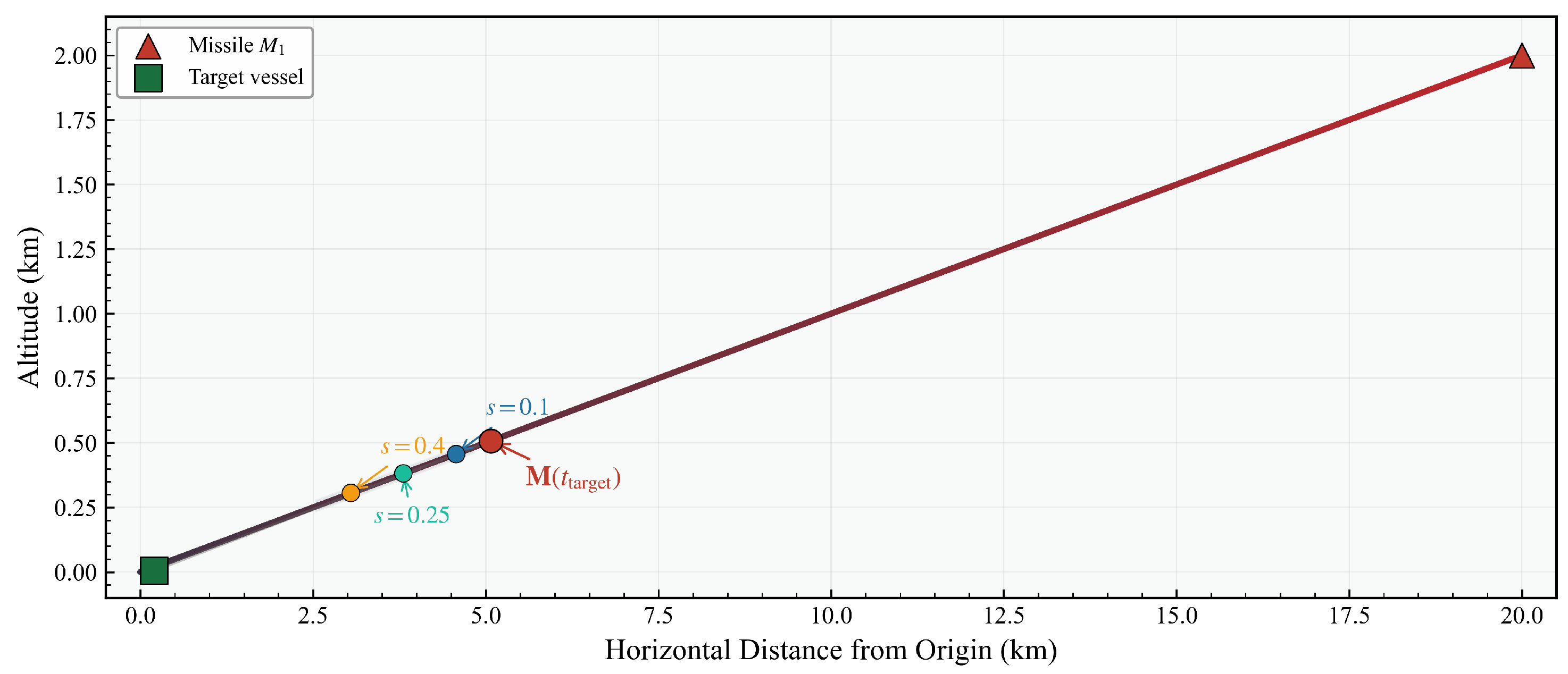
Geometric interpretation of the inverse design parameters. The target interception time determines the missile position along its trajectory (red), while the offset parameter s positions the desired burst point along the missile–target line.
Figure 4.
Geometric interpretation of the inverse design parameters. The target interception time determines the missile position along its trajectory (red), while the offset parameter s positions the desired burst point along the missile–target line.
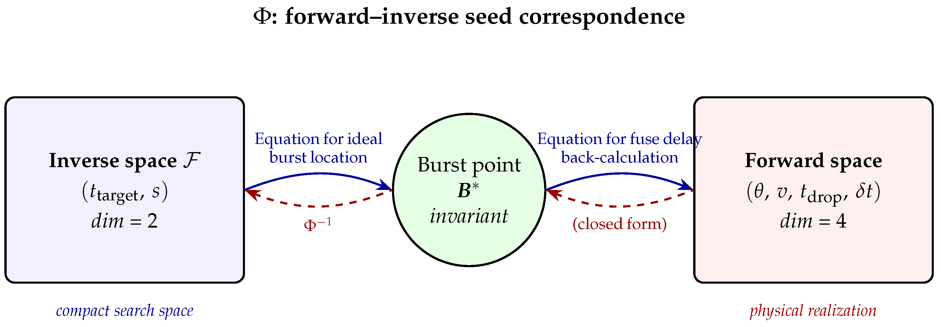
Figure 5.
Schematic of the forward–inverse correspondence established in Proposition 1. The two-dimensional inverse seed space (left) and the four-dimensional physical agent parameter space (right) communicate via the burst point (middle), which plays the role of an invariant within the line-of-sight-aligned seed family. The correspondence is used to construct feasible seeds; the subsequent Nelder–Mead refinement is performed in the physical parameter space.
Figure 5.
Schematic of the forward–inverse correspondence established in Proposition 1. The two-dimensional inverse seed space (left) and the four-dimensional physical agent parameter space (right) communicate via the burst point (middle), which plays the role of an invariant within the line-of-sight-aligned seed family. The correspondence is used to construct feasible seeds; the subsequent Nelder–Mead refinement is performed in the physical parameter space.
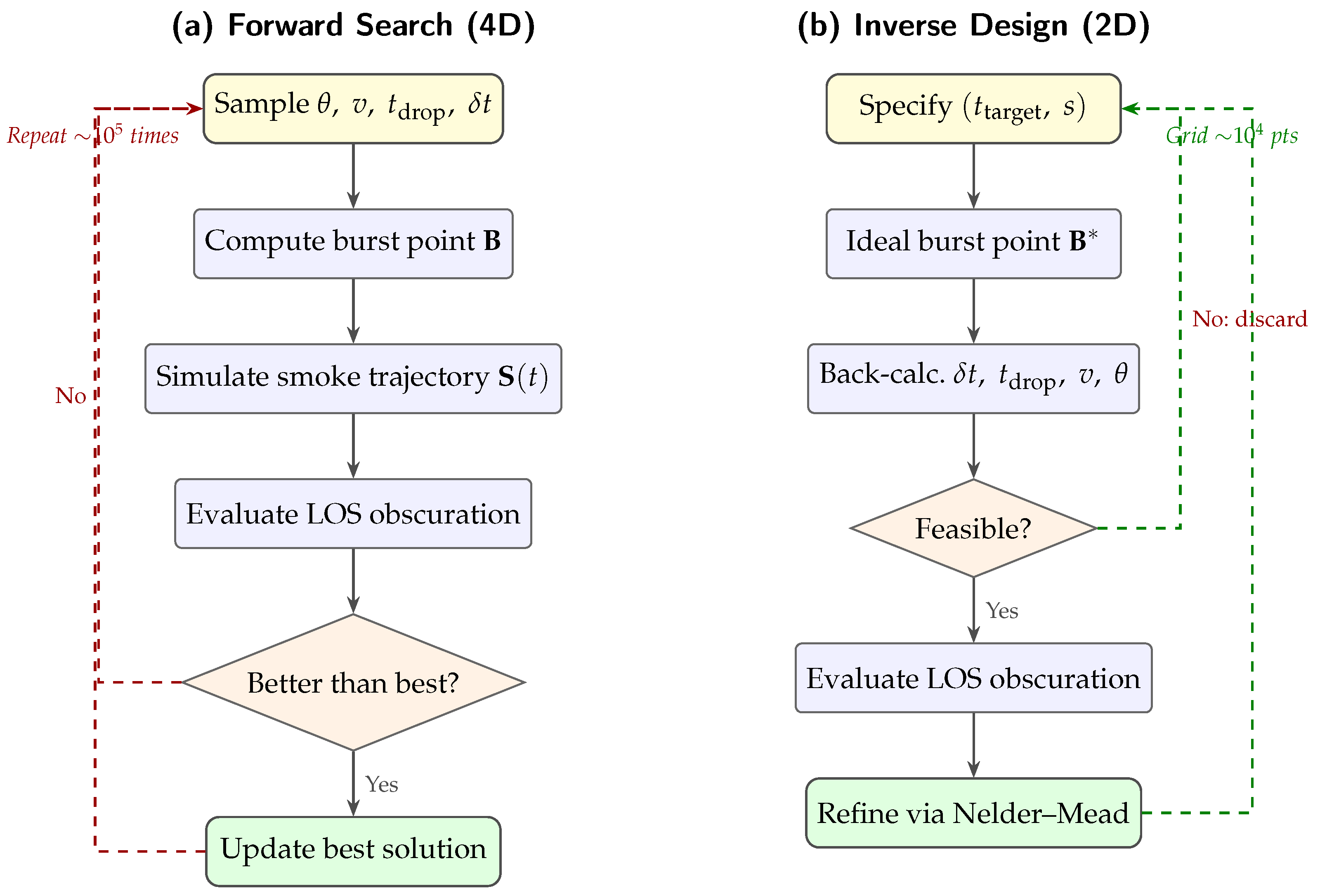
Figure 6.
Comparison of the forward search (a) and inverse-seeded approach (b). The forward method searches a 4D parameter space and evaluates each candidate, while the inverse stage specifies the desired smoke location in a 2D space, analytically back-calculates feasible UAV parameters, and passes them to a physical-space Nelder–Mead refinement.
Figure 6.
Comparison of the forward search (a) and inverse-seeded approach (b). The forward method searches a 4D parameter space and evaluates each candidate, while the inverse stage specifies the desired smoke location in a 2D space, analytically back-calculates feasible UAV parameters, and passes them to a physical-space Nelder–Mead refinement.
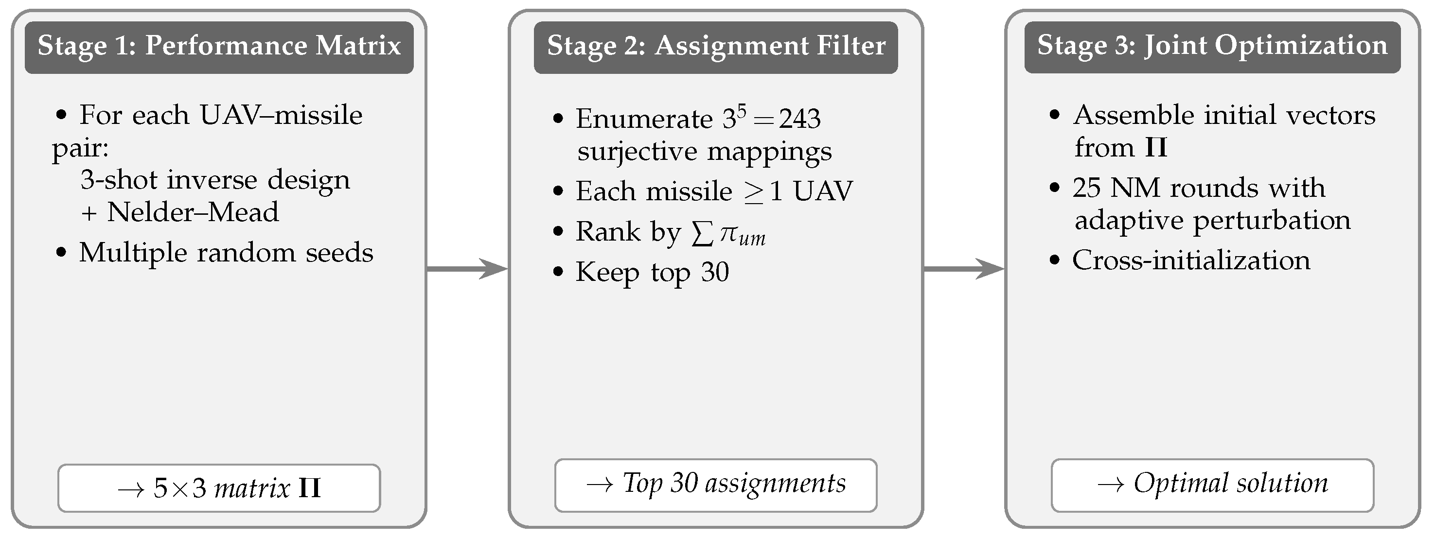
Figure 7.
Hierarchical three-stage framework for multi-UAV multi-missile smoke screen allocation. Stage 1 builds an independent performance matrix, Stage 2 enumerates and filters candidate assignments, and Stage 3 jointly optimizes the selected assignments with cross-initialization.
Figure 7.
Hierarchical three-stage framework for multi-UAV multi-missile smoke screen allocation. Stage 1 builds an independent performance matrix, Stage 2 enumerates and filters candidate assignments, and Stage 3 jointly optimizes the selected assignments with cross-initialization.
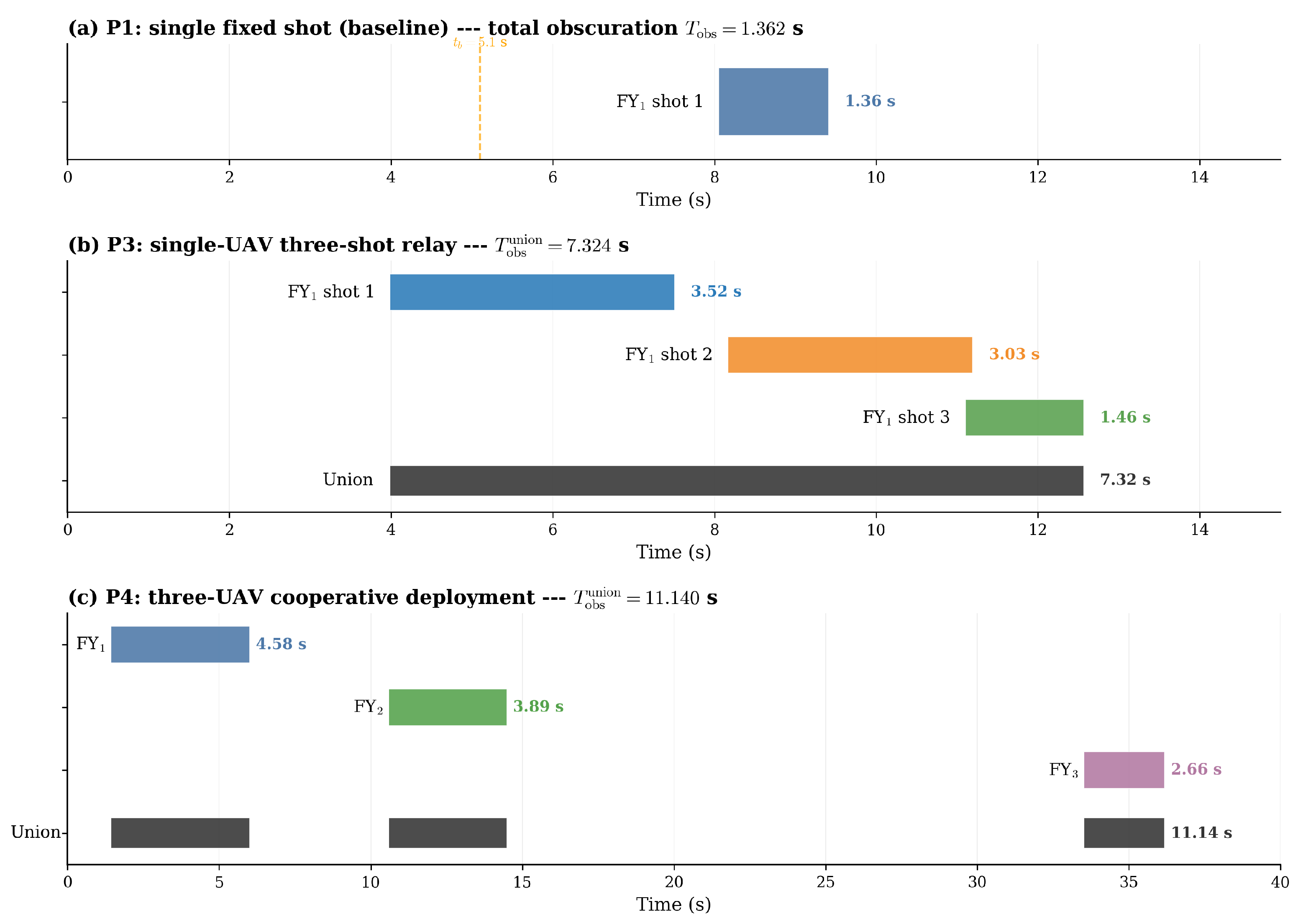
Figure 8.
Obscuration timelines for the first three sub-problems. (a) P1 baseline with a single fixed shot from against (total ); the dashed vertical line marks the burst time . (b) P3 three-shot relay from against : the three individual windows exhibit modest pairwise overlap and their union (dark row) spans . (c) P4 cooperative deployment in which three UAVs each release one projectile, producing three essentially disjoint windows whose union (dark row) reaches .
Figure 8.
Obscuration timelines for the first three sub-problems. (a) P1 baseline with a single fixed shot from against (total ); the dashed vertical line marks the burst time . (b) P3 three-shot relay from against : the three individual windows exhibit modest pairwise overlap and their union (dark row) spans . (c) P4 cooperative deployment in which three UAVs each release one projectile, producing three essentially disjoint windows whose union (dark row) reaches .
Figure 9.
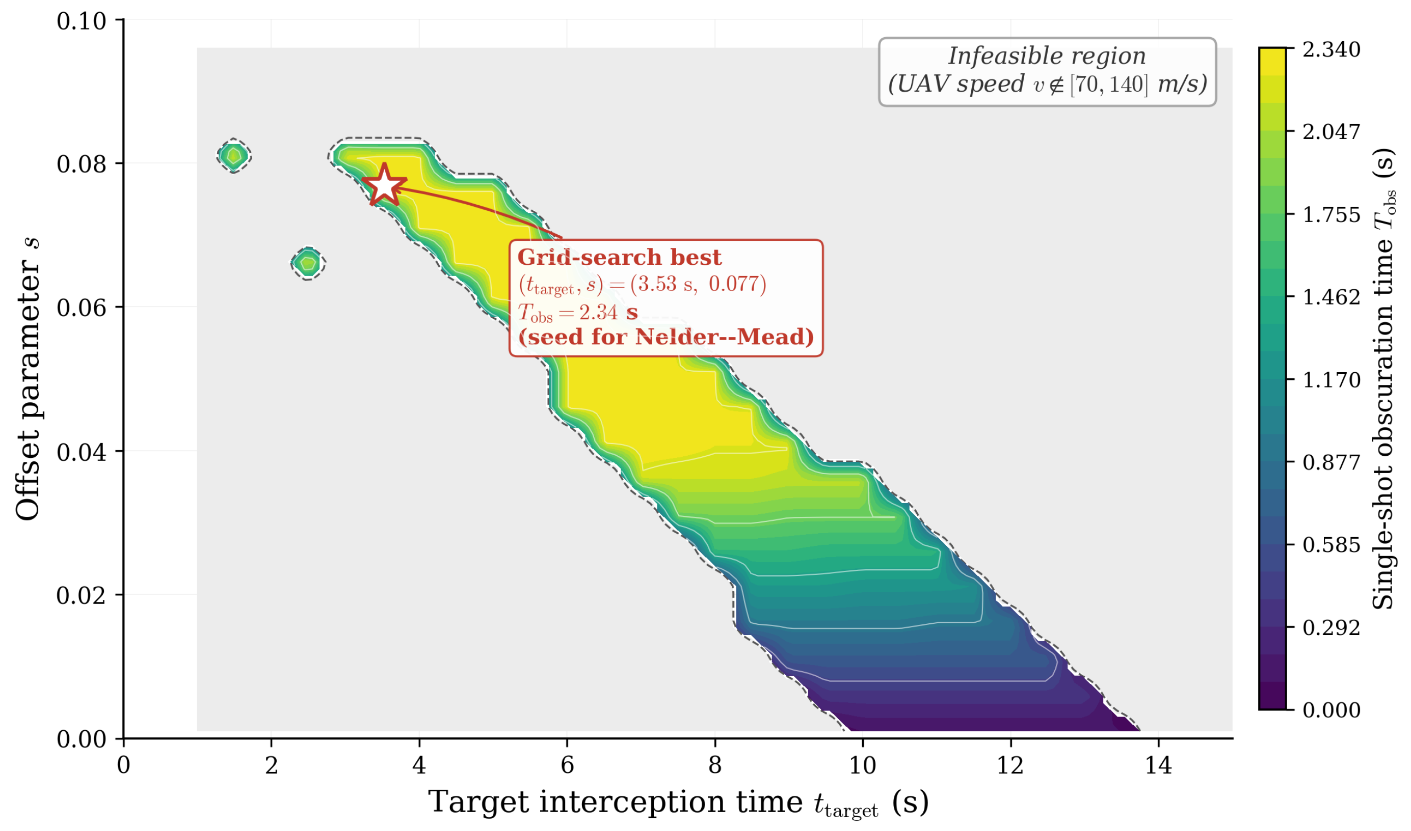
Inverse design search landscape for . The heatmap shows single-shot obscuration time over the parameter space. The feasible region (colored band) is confined by UAV speed constraints; the gray region is infeasible. The star marks the grid-search best—the maximum value attained on the discrete sampling grid, which serves as the seed for the subsequent multi-start Nelder–Mead refinement; the refined best value reported in the text is .
Figure 9.
Inverse design search landscape for . The heatmap shows single-shot obscuration time over the parameter space. The feasible region (colored band) is confined by UAV speed constraints; the gray region is infeasible. The star marks the grid-search best—the maximum value attained on the discrete sampling grid, which serves as the seed for the subsequent multi-start Nelder–Mead refinement; the refined best value reported in the text is .
Figure 10.
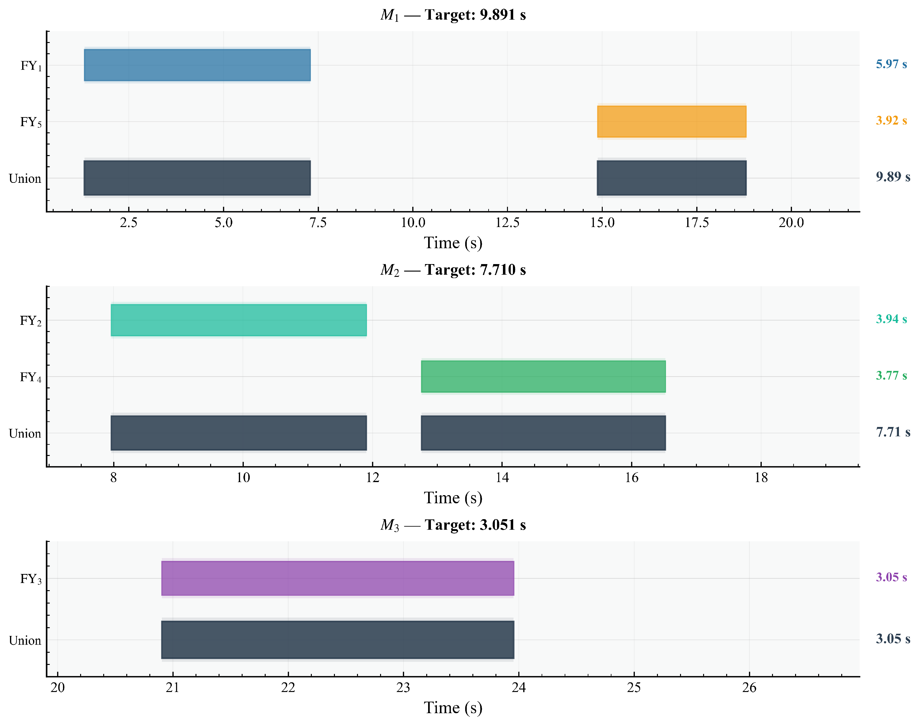
P5 obscuration timelines for each missile. Each subplot shows the contributions from assigned UAVs (colored bars, with each UAV’s three projectiles shown individually) and the union (dark region). Total obscuration: , , , grand total = .
Figure 10.
P5 obscuration timelines for each missile. Each subplot shows the contributions from assigned UAVs (colored bars, with each UAV’s three projectiles shown individually) and the union (dark region). Total obscuration: , , , grand total = .
Figure 11.
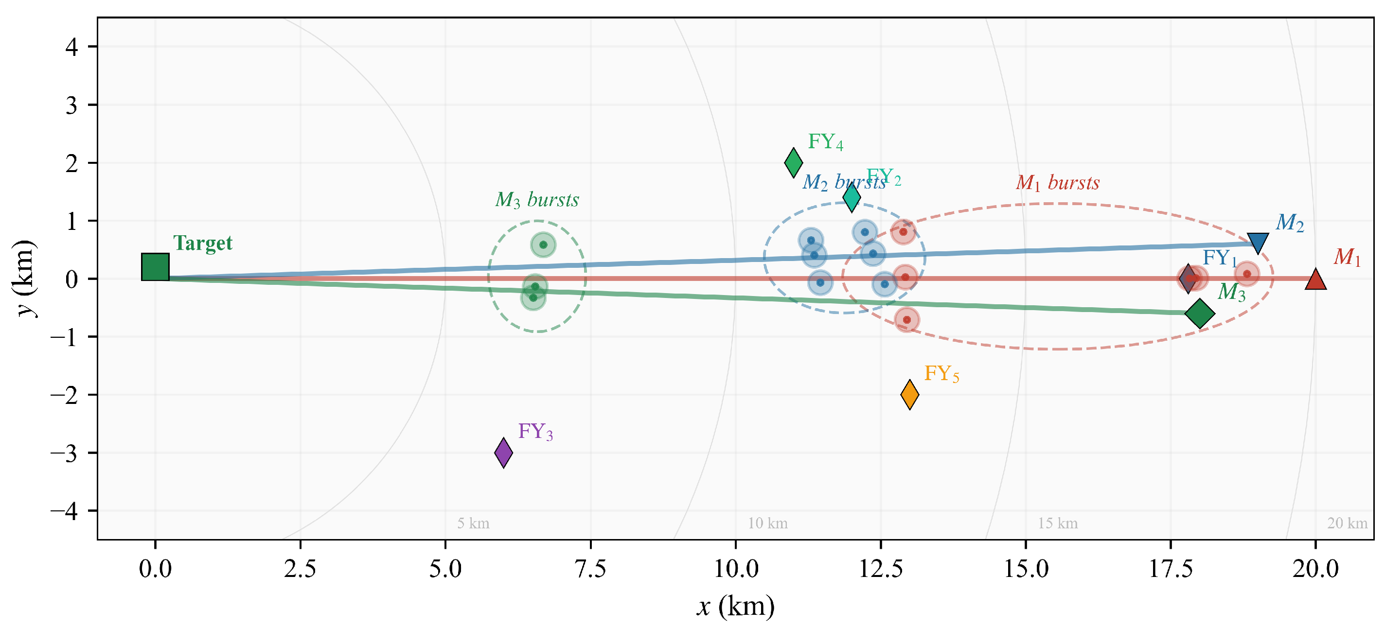
Top-down (-plane) view of the P5 optimal solution. Missile trajectories are shown as colored lines converging on the target (green square); diamond markers indicate UAV initial positions. Semi-transparent circles represent the 15 burst points, color-coded by target missile (: red; : blue; : green), with dashed ellipses enclosing each missile’s burst cluster. Range rings indicate distance from the decoy.
Figure 11.
Top-down (-plane) view of the P5 optimal solution. Missile trajectories are shown as colored lines converging on the target (green square); diamond markers indicate UAV initial positions. Semi-transparent circles represent the 15 burst points, color-coded by target missile (: red; : blue; : green), with dashed ellipses enclosing each missile’s burst cluster. Range rings indicate distance from the decoy.
Figure 12.
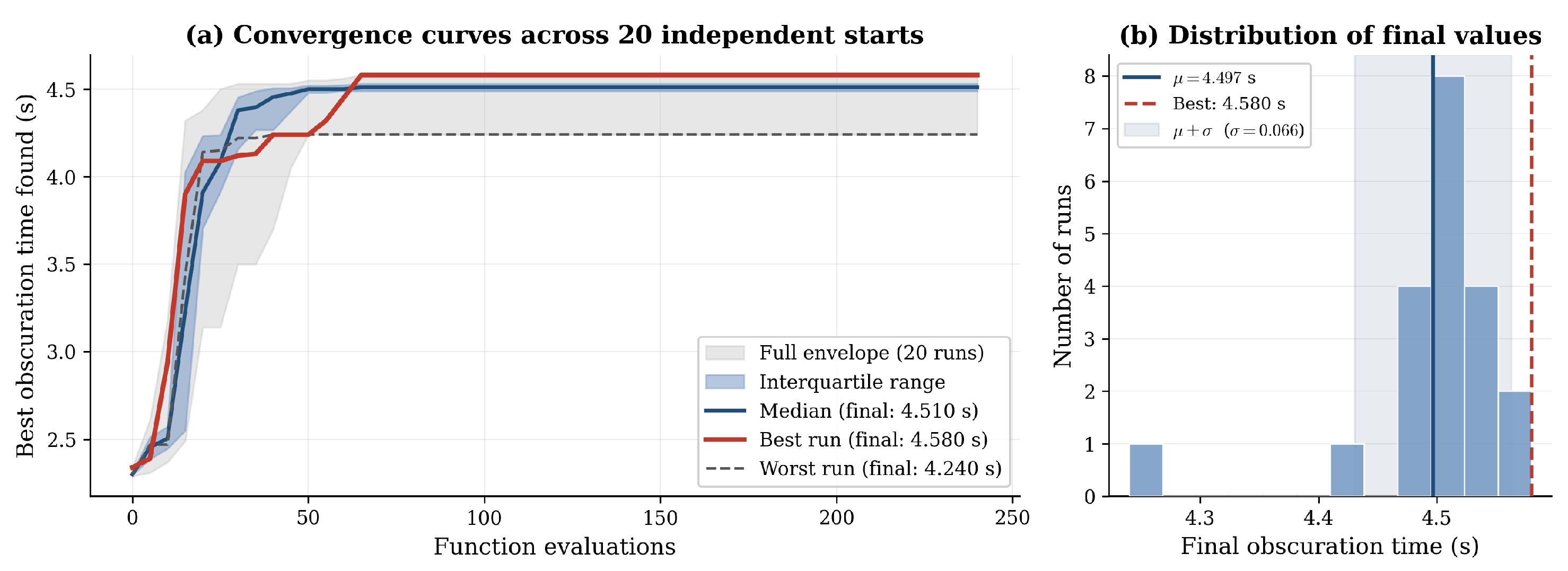
Multi-start Nelder–Mead convergence analysis for (P2). (a) Running-best convergence curves for 20 independent starts; the best, median, and worst runs are highlighted. (b) Distribution of final objective values with mean and standard deviation .
Figure 12.
Multi-start Nelder–Mead convergence analysis for (P2). (a) Running-best convergence curves for 20 independent starts; the best, median, and worst runs are highlighted. (b) Distribution of final objective values with mean and standard deviation .
Figure 13.
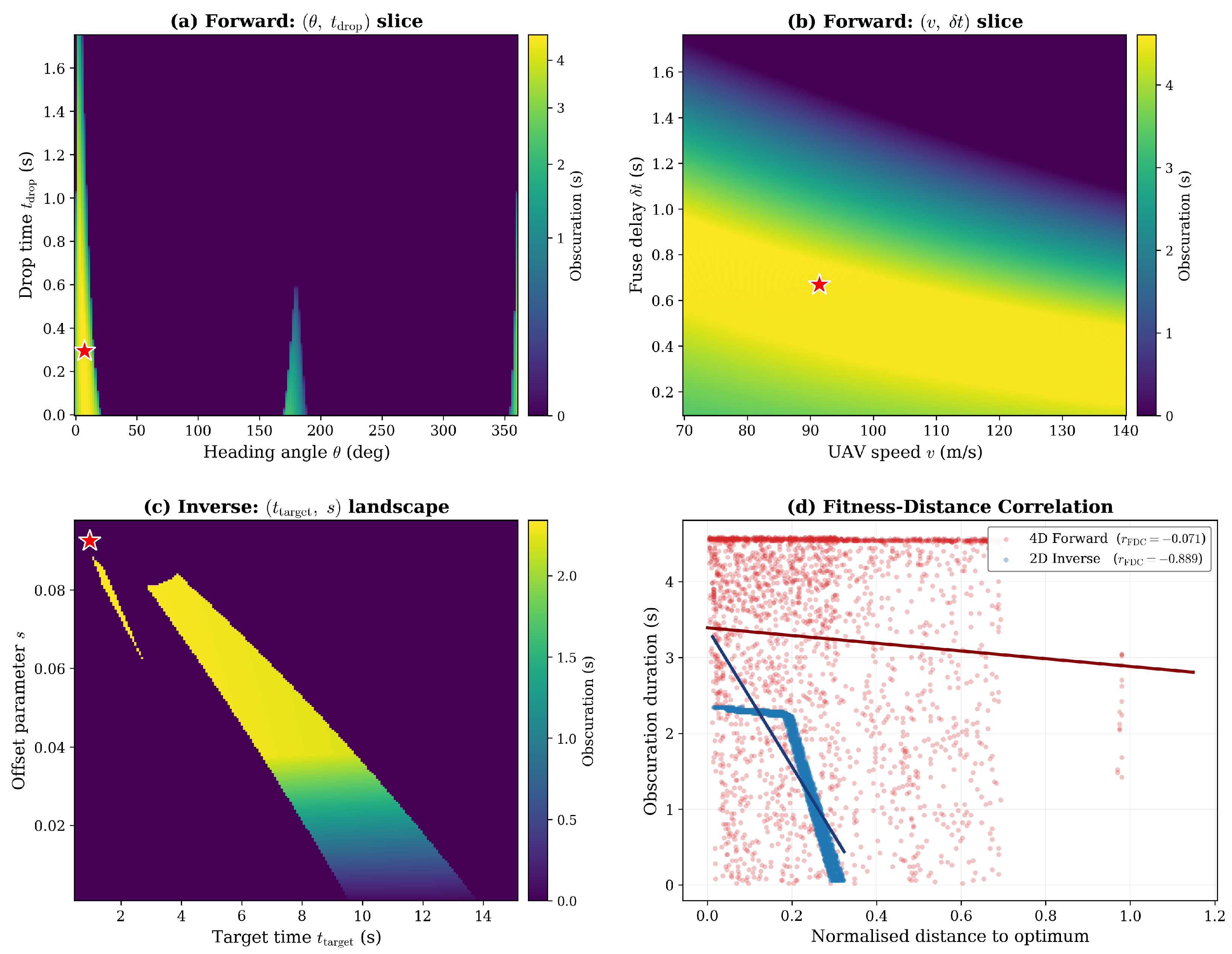
Comparison of the objective landscape in forward and inverse parameterizations (P2 problem, FY1 ). All panels are zoomed to the bounding box of the feasible region. (a) Forward slice with v and fixed at the best refined values, showing sparse and fragmented feasibility across heading angles. (b) Forward slice with and fixed, revealing a narrow diagonal feasible band. (c) Inverse landscape exhibiting a single smooth peak with concentric gradient. (d) Fitness-Distance Correlation: the 2D inverse space () shows a strong negative correlation, whereas the 4D forward space () shows negligible correlation. Red stars mark the best sampled/refined point.
Figure 13.
Comparison of the objective landscape in forward and inverse parameterizations (P2 problem, FY1 ). All panels are zoomed to the bounding box of the feasible region. (a) Forward slice with v and fixed at the best refined values, showing sparse and fragmented feasibility across heading angles. (b) Forward slice with and fixed, revealing a narrow diagonal feasible band. (c) Inverse landscape exhibiting a single smooth peak with concentric gradient. (d) Fitness-Distance Correlation: the 2D inverse space () shows a strong negative correlation, whereas the 4D forward space () shows negligible correlation. Red stars mark the best sampled/refined point.
Table 1.
Physical parameters and initial conditions for the smoke screen deployment scenario.
Table 1.
Physical parameters and initial conditions for the smoke screen deployment scenario.
| Parameter | Value | Description |
|---|
| g | | Gravitational acceleration |
| 300 | Missile speed |
| v | 70–140 m/s | UAV speed range |
| | Smoke cloud sinking speed |
| 10 m | Effective smoke radius |
| 20 s | Smoke effective duration |
| 7 m | Target vessel radius |
| 10 m | Target vessel height |
| Missile initial positions (m) |
| | |
| | |
| | |
| UAV initial positions (m) |
| | |
| | |
| | |
| | |
| | |
Table 2.
Summary of the five sub-problems in the smoke screen optimization hierarchy.
Table 2.
Summary of the five sub-problems in the smoke screen optimization hierarchy.
| Problem | UAVs | Missiles | Shots/UAV | Decision Variables |
|---|
| P1 | 1 (FY1) | 1 () | 1 | 0 (fixed) |
| P2 | 1 (FY1) | 1 () | 1 | 4: |
| P3 | 1 (FY1) | 1 () | 3 | 8: |
| P4 | 3 (FY1–3) | 1 () | 1 each | 12: |
| P5 | 5 (FY1–5) | 3 () | 3 each | Assignment + 40 continuous |
Table 3.
Optimized parameters for the P3 three-shot relay ().
Table 3.
Optimized parameters for the P3 three-shot relay ().
| Shot | (s) | (s) | (s) | Burst Point (m) | Single Obs. (s) |
|---|
| 1 | 0.172 | 3.813 | 3.985 | (17,243, 4, 1729) | 3.522 |
| 2 | 3.093 | 5.072 | 8.165 | (16,660, 7, 1674) | 3.027 |
| 3 | 5.175 | 5.930 | 11.105 | (16,249, 10, 1628) | 1.463 |
| Total union obscuration | 7.324 |
Table 4.
Optimized parameters for the P4 three-UAV cooperative deployment against .
Table 4.
Optimized parameters for the P4 three-UAV cooperative deployment against .
| UAV | (deg) | v (m/s) | (s) | (s) | Burst Point (m) | Single Obs. (s) |
|---|
| 5.75 | 72.88 | 0.693 | 0.737 | (17,904, 10, 1797) | 4.581 |
| 265.82 | 127.59 | 4.178 | 6.416 | (11,902, 52, 1198) | 3.894 |
| 75.31 | 93.87 | 32.481 | 1.036 | | 2.664 |
| Total union obscuration | 11.140 |
Table 5.
Performance matrix (seconds): maximum three-shot obscuration duration for each UAV–missile pair, computed independently.
Table 5.
Performance matrix (seconds): maximum three-shot obscuration duration for each UAV–missile pair, computed independently.
| | | | |
|---|
| 5.98 | 0.00 | 0.00 |
| 3.96 | 3.96 | 3.72 |
| 3.14 | 3.02 | 3.06 |
| 3.82 | 3.78 | 3.54 |
| 3.94 | 3.60 | 3.76 |
Table 6.
Minimum speed required for to generate a feasible inverse design seed under .
Table 6.
Minimum speed required for to generate a feasible inverse design seed under .
| Pair | Minimum Required Speed (m/s) | Operational Limit (m/s) | Outcome |
|---|
| 0.17 | 70–140 | Feasible after speed lower-bound filtering |
| 177.12 | 70–140 | Infeasible |
| 282.14 | 70–140 | Infeasible |
Table 7.
Complete P5 deployment parameters for all 15 projectiles under the optimal assignment .
Table 7.
Complete P5 deployment parameters for all 15 projectiles under the optimal assignment .
| Target | UAV | Shot | (deg) | v (m/s) | (s) | (s) | Burst Point (m) |
|---|
| | 1 | 4.53 | 99.92 | 0.100 | 0.129 | |
| 2 | 4.53 | 99.92 | 1.101 | 0.226 | |
| 3 | 4.53 | 99.92 | 8.659 | 1.503 | |
| 1 | 92.20 | 139.63 | 7.969 | 1.303 | |
| 2 | 92.20 | 139.63 | 14.431 | 0.101 | |
| 3 | 92.20 | 139.63 | 18.579 | 1.537 | |
| | 1 | 290.74 | 135.76 | 2.274 | 2.451 | |
| 2 | 290.74 | 135.76 | 5.326 | 2.263 | |
| 3 | 290.74 | 135.76 | 9.978 | 1.822 | |
| 1 | 282.51 | 130.49 | 0.101 | 10.403 | |
| 2 | 282.51 | 130.49 | 2.057 | 10.476 | |
| 3 | 282.51 | 130.49 | 6.060 | 10.182 | |
| | 1 | 79.20 | 139.91 | 18.175 | 1.249 | |
| 2 | 79.20 | 139.91 | 20.177 | 0.677 | |
| 3 | 79.20 | 139.91 | 24.986 | 1.082 | |
| subtotal: 9.891 s subtotal: 7.710 s subtotal: 3.051 s |
| Grand total: 20.652 s |
Table 8.
P5 obscuration totals under three comparison scenarios (cylindrical evaluator, ).
Table 8.
P5 obscuration totals under three comparison scenarios (cylindrical evaluator, ).
| Scenario | Description | Total (s) |
|---|
| One-UAV-per-missile baseline | Best Stage 1 entry per missile column of ; three UAVs, nine projectiles | 13.00 |
| Same assignment, Stage 1 assembly | Assignment ; union of Stage 1 relay solutions, no Stage 3 joint refinement | 20.67 |
| Stage 3 joint optimum | Assignment after per-missile joint multi-start refinement | 20.652 |
Table 9.
Summary of results and computational characteristics for all sub-problems.
Table 9.
Summary of results and computational characteristics for all sub-problems.
| Problem | Obscuration (s) | Decision Dim. | Inverse Dim. | Approx. Runtime |
|---|
| P1 | 1.362 | 0 (fixed) | — | <1 s |
| P2 | 4.580 | 4 | 2 seed + 4D NM | ∼5 s |
| P3 | 7.324 | 8 | 2 + NM | ∼30 s |
| P4 | 11.140 | 12 | + NM | ∼2 min |
| P5 | 20.652 | 40 + assignment | + NM | ∼15 min |
Table 10.
Comparison of optimization strategies on the P2 problem (, single shot, cylinder model). Each method is run five times with different seeds; best, mean, standard deviation, average function evaluations, wall time, and a two-sided Mann–Whitney comparison against the proposed method are reported.
Table 10.
Comparison of optimization strategies on the P2 problem (, single shot, cylinder model). Each method is run five times with different seeds; best, mean, standard deviation, average function evaluations, wall time, and a two-sided Mann–Whitney comparison against the proposed method are reported.
| Method | Search Dim. | Best Obs. (s) | Mean Obs. (s) | Func. Evals | Wall Time (s) | p vs. Proposed |
|---|
| 4D Random Search () | 4 | 4.570 | 4.252 ± 0.316 | 100,000 | 24.85 | 0.0075 |
| 4D DE + Nelder–Mead | 4 | 4.590 | 4.568 ± 0.027 | 11,364 | 40.51 | 0.6513 |
| 2D Inverse Seed + 4D Nelder–Mead | 2 seed + 4D NM | 4.580 | 4.580 ± 0.000 | 9846 | 2.75 | — |
Table 11.
Budget-matched high-dimensional comparison for P3 and P4. Values are based on three independent seeds and the same cylindrical target evaluator; function evaluations and wall times are averages.
Table 11.
Budget-matched high-dimensional comparison for P3 and P4. Values are based on three independent seeds and the same cylindrical target evaluator; function evaluations and wall times are averages.
| Problem | Method | Best Obs. (s) | Mean Obs. (s) | Func. Evals | Wall Time (s) |
|---|
| P3 (8D) | Direct random search | 4.260 | 2.430 ± 1.546 | 5000 | 2.08 |
| P3 (8D) | 8D DE + Nelder–Mead | 0.000 | 0.000 ± 0.000 | 928 | 0.17 |
| P3 (8D) | Inverse seed + 8D Nelder–Mead | 7.380 | 7.340 ± 0.037 | 2058 | 0.71 |
| P4 (12D) | Direct random search | 4.050 | 3.430 ± 0.588 | 5000 | 2.54 |
| P4 (12D) | 12D DE + Nelder–Mead | 0.000 | 0.000 ± 0.000 | 1940 | 0.93 |
| P4 (12D) | Inverse seed + 12D Nelder–Mead | 11.160 | 11.130 ± 0.042 | 2095 | 1.11 |
Table 12.
Snapshot sensitivity of the P5 solution to the inverse design offset threshold . The table retains only final-solution shots whose projection onto the corresponding missile–target line lies within and recomputes union obscuration.
Table 12.
Snapshot sensitivity of the P5 solution to the inverse design offset threshold . The table retains only final-solution shots whose projection onto the corresponding missile–target line lies within and recomputes union obscuration.
| Retained Shots | (s) | (s) | (s) | Total (s) |
|---|
| 0.20 | | 9.89 | 0.00 | 0.00 | 9.89 |
| 0.25 | | 9.89 | 0.00 | 0.00 | 9.89 |
| 0.35 | | 9.89 | 7.70 | 0.00 | 17.59 |
| 0.50 | | 9.89 | 7.70 | 3.05 | 20.64 |
Table 13.
Sensitivity of the rounded P5 deployment to wind drift and missile trajectory prediction errors. Values are recomputed with the same deployment parameters and cylindrical LOS evaluator.
Table 13.
Sensitivity of the rounded P5 deployment to wind drift and missile trajectory prediction errors. Values are recomputed with the same deployment parameters and cylindrical LOS evaluator.
| Evaluation Scenario | (s) | (s) | (s) | Total (s) |
|---|
| Nominal rounded P5 parameters | 9.89 | 7.70 | 3.05 | 20.64 |
| Wind m/s | 9.81 | 7.60 | 2.98 | 20.39 |
| Wind m/s | 9.25 | 6.42 | 2.55 | 18.22 |
| Wind m/s | 7.59 | 5.37 | 2.17 | 15.13 |
| Missile lateral bias in y | 2.13 | 1.31 | 2.32 | 5.76 |
| Missile range bias in x | 7.83 | 6.02 | 3.00 | 16.85 |
| Missile altitude bias in z | 0.00 | 0.00 | 1.61 | 1.61 |