Article

Representation-Level Temporal–Frequency Symmetric Learning for Battery State-of-Charge Estimation and Voltage Reconstruction

School of Mathematics and Statistics, Zhengzhou University, Zhengzhou 450001, China
*
Author to whom correspondence should be addressed.
Symmetry 2026, 18(6), 931; https://doi.org/10.3390/sym18060931 (registering DOI)
Submission received: 18 April 2026 / Revised: 20 May 2026 / Accepted: 25 May 2026 / Published: 29 May 2026
(This article belongs to the Section Engineering and Materials)

Abstract

Accurate battery state-of-charge (SOC) estimation under dynamic operating conditions remains challenging because battery responses are nonlinear, history-dependent, temperature-sensitive, and prone to transient disturbances. To address this problem, this paper proposes a representation-level temporal–frequency symmetry framework, termed the Joint Temporal–Frequency Cross-Domain Attention Network (JTFCD-Net), for joint SOC estimation and voltage reconstruction. Here, symmetry denotes aligned latent representations rather than physical invariance: temporal and frequency-aware views are derived from the same battery process, mapped into the same latent space, and kept at identical temporal resolution and hidden dimensionality. A temporal aggregation block extracts local dynamics at multiple receptive fields, and a Temporal Attention Aggregation Module (TAAM) captures long-range dependence. A Frequency-Aware Attention Module (FAM) then uses global spectral statistics to perform lightweight channel recalibration, thereby injecting coarse frequency-domain information into the temporal representation while preserving the hidden feature shape. A Cross-Domain Attention Module (CDAM) performs bidirectional cross-attention, allowing the two views to query and exchange information. The fused representation is decoded by a main SOC head and an auxiliary voltage reconstruction head, which preserves voltage-response dynamics in the shared representation. Experiments on the CALCE A123 benchmark under multiple fixed ambient temperatures and operating conditions show that JTFCD-Net yields consistently lower errors than the selected baseline methods, while ablation studies confirm the contribution of cross-domain fusion and auxiliary voltage supervision. External validation on the NASA Ames battery aging dataset is also conducted as an independent laboratory-scale cell benchmark. These results indicate that combining temporal modeling with frequency-aware representation learning is a promising direction, although deployment value still requires validation in real BMS settings.

1. Introduction

Accurate state-of-charge (SOC) estimation is a core function of battery management systems because it directly affects energy scheduling, safety protection, remaining-range prediction, and charge–discharge optimization in electric vehicles and stationary energy-storage systems [1,2,3]. However, SOC cannot be measured directly and must be inferred from observable quantities such as terminal voltage, current, and temperature. This inverse problem is difficult because lithium-ion batteries exhibit strong nonlinearity, temperature dependence, hysteresis, relaxation behavior, and aging-related drift [4,5,6]. Under dynamic load profiles, similar voltage values may correspond to different hidden SOC states if the preceding current history is different, which makes reliable online estimation particularly challenging.
Traditional SOC estimation methods are mainly based on open-circuit-voltage relationships, equivalent-circuit models, electrochemical models, and recursive filtering algorithms [7,8,9,10,11]. These methods remain important because they offer clear physical interpretation and practical deployability. Nevertheless, their performance is often sensitive to modeling assumptions, parameter identification quality, and operating-condition mismatch [2,4,12]. When temperature, load profile, and degradation state vary together, maintaining a uniformly reliable model becomes increasingly difficult, which has motivated the rapid development of data-driven SOC estimation methods.
Recent deep learning approaches have improved SOC estimation by learning nonlinear mappings directly from battery measurement sequences [13,14,15]. Recurrent models such as GRU and LSTM are effective for sequential dependency modeling [16,17,18], while hybrid structures including CNN-LSTM, attention-LSTM, U-Net-CNN, BiGRU, and multi-branch architectures further improve local feature extraction and dynamic modeling capacity [19,20,21,22,23,24]. In addition, learning-based frameworks have been combined with Kalman filtering or observer mechanisms to improve robustness and physical plausibility [25,26,27,28,29]. Despite this progress, many existing estimators still rely primarily on temporal modeling, while spectral information often remains weakly explored rather than systematically integrated. As a result, the learned representation may not fully capture the latent battery dynamics needed for robust SOC estimation under highly dynamic conditions.
This limitation matters because battery responses contain complementary information in both time and frequency views. In the time domain, SOC evolution relates to local transients, long-range operating history, and temperature-coupled relaxation. In the frequency domain, the same sequence contains short-window spectral patterns related to local trend variations, transient polarization, and measurement disturbances. Here, the frequency view is used for learnable latent recalibration rather than handcrafted spectral augmentation. In this work, temporal–frequency symmetry is used in a representation-level sense, not as physical invariance, duality, or reversibility. The two views originate from the same battery process, are mapped to the same latent space, keep matched temporal resolution and hidden width, and interact bidirectionally. Existing methods rarely maintain this aligned space, and auxiliary voltage reconstruction is still underused for preserving voltage-response morphology [30,31,32,33,34,35].
To address these issues, this paper proposes the Joint Temporal–Frequency Cross-Domain Attention Network (JTFCD-Net) for simultaneous SOC estimation and voltage reconstruction. The model first extracts multi-scale local dynamics and long-range temporal dependence. A frequency-aware branch is generated from the same latent sequence and returned to the same hidden space, so temporal and frequency-aware representations form an aligned pair with identical temporal resolution and hidden dimension. CDAM enables the two views to query each other through bidirectional attention rather than shallow concatenation. Finally, voltage reconstruction constrains the shared backbone to preserve useful voltage-response dynamics.
Compared with sequence models that rely mainly on temporal dependency modeling, the proposed framework realizes representation-level temporal–frequency symmetry through shared-space mapping, reciprocal cross-domain interaction, and reliability-oriented multi-task supervision.

Contributions

The main contributions of this work are summarized as follows:
  • We propose JTFCD-Net, a unified SOC estimation architecture that integrates temporal modeling, global spectral-statistics-based recalibration, cross-domain interaction, and voltage reconstruction supervision within a representation-level temporal–frequency framework.
  • We design CDAM to realize reciprocal querying between the two aligned representations, enabling information exchange beyond conventional feature concatenation.
  • We introduce full-window voltage reconstruction as auxiliary supervision and verify that JTFCD-Net achieves consistently lower SOC errors than selected baselines across fixed ambient temperatures and operating conditions.

2. Related Work

2.1. Model-Based SOC Estimation

Model-based SOC estimation methods have long been regarded as a fundamental research direction in battery management because of their clear physical interpretation and suitability for online implementation. Early studies widely adopted OCV-based mapping and equivalent-circuit formulations to establish the relationship between SOC and measurable electrical variables [7,8]. On top of these battery models, recursive estimation algorithms such as the extended Kalman filter, unscented Kalman filter, and their improved variants have been extensively developed to estimate SOC under noisy and time-varying operating conditions [5,9,12,36,37]. In addition, enhanced ECM-based identification strategies and electrochemical model-based state estimators have been proposed to improve physical fidelity and parameter adaptability [10,11].
Despite their practical value, model-based methods still face several limitations. Their accuracy depends strongly on the validity of modeling assumptions, the quality of parameter identification, and the consistency between offline calibration and online operating conditions [2,4]. When batteries operate across variable temperatures, load profiles, and aging stages, it becomes increasingly difficult to maintain a fixed model structure with uniformly reliable parameters. These limitations have motivated the rapid development of data-driven and hybrid learning methods.

2.2. Data-Driven and Hybrid SOC Estimation

Data-driven SOC estimation methods seek to learn the nonlinear mapping from measured battery signals to SOC labels directly from data. Conventional neural-network estimators already demonstrated the feasibility of learning SOC from voltage, current, and temperature sequences without explicit electrochemical equations [38]. Subsequently, recurrent models such as GRU, LSTM, and clockwork RNN became popular because battery measurements are inherently sequential and temporally dependent [16,17,18,39,40]. To further improve feature extraction, researchers introduced CNN-LSTM pipelines, attention-enhanced LSTM models, and constrained-input or extended-input recurrent networks, which improved estimation accuracy under dynamic conditions and multiple operating factors [19,20,41,42].
More recently, hybrid architectures have become increasingly important. CNN-based encoders, temporal convolution networks, U-Net-like designs, and multi-branch recurrent hybrids have been used to improve local feature extraction and multi-scale representation learning [21,23,24,43]. At the same time, several studies have integrated deep learning with Kalman filtering, adaptive observers, or model-based correction mechanisms, aiming to combine nonlinear representation learning with recursive estimation robustness [25,26,27,28,29]. Although these approaches have produced substantial progress, many of them still rely on a predominantly temporal description of the input sequence and are optimized mainly for a single SOC target, leaving room for richer feature interaction and auxiliary physically grounded supervision.

2.3. Attention and Transformer-Based Battery State Estimation

Attention mechanisms and Transformer-based architectures provide a more flexible way to model long-range dependencies than conventional recurrent networks, and they have therefore attracted growing interest in battery state estimation research [30,31,32]. Self-supervised Transformer models have shown that attention-based architectures can learn informative battery representations from sequential operational data [30]. Observer-coupled Transformer estimators further demonstrate the potential of combining global sequence modeling with system-theoretic constraints [31]. In addition, hybrid Transformer-LSTM models and attention-enhanced multi-state estimation frameworks indicate that attention can be especially useful when the estimation problem involves strong operating-condition variability and long-range temporal dependency [22,24,33].
At the same time, recent studies suggest two trends that are highly relevant to the present study. First, structured inductive bias can improve robustness under varying operating conditions [34]. Second, joint-estimation strategies demonstrate that learning multiple correlated battery states can improve observability and information utilization [35]. However, existing attention-based SOC methods still rarely incorporate explicit frequency-aware modeling, and cross-domain interaction between temporal and spectral representations remains insufficiently explored. Moreover, the integration of voltage reconstruction as an auxiliary task within an attention-driven SOC framework is still limited. These observations motivate the development of the proposed JTFCD-Net, which jointly models temporal dynamics, spectral characteristics, cross-domain feature interaction, and voltage-consistent multi-task supervision.

3. Methodology

In this paper, the proposed framework is termed the Joint Temporal–Frequency Cross-Domain Attention Network (JTFCD-Net). Here, temporal–frequency symmetry is defined at the representation level rather than as physical invariance, duality, or reversibility. The temporal feature  H ( t )  and frequency-aware feature  H ( f )  are derived from the same battery window, mapped to the same latent space, and kept with identical temporal resolution and hidden width. Their symmetry is therefore realized by matched representation status and reciprocal cross-domain attention.
The framework is further designed under a dual-task learning paradigm, where the primary task is SOC estimation and the auxiliary task is voltage reconstruction. This design is intended to improve the reliability of SOC estimation by preserving informative voltage-response dynamics in the shared representation. For a sliding window ending at time step k, the multivariate battery input is denoted as
X k = [ x k L + 1 , x k L + 2 , , x k ] R L × d 0 ,
where L is the window length and  d 0  is the number of measured or derived input variables. In a typical setting,  x t  may contain terminal voltage, current, temperature, and optional differential features. Unless otherwise stated, all hidden features are organized row-wise along the temporal dimension, meaning that each row corresponds to one time step inside the observation window. For clarity, the batch dimension is omitted throughout the derivation. Under this notation, the dimensional consistency of each module can be checked directly by following the shape of the feature matrix from one transformation to the next. For symbol consistency,  H ( t ) H ( f ) , and  H ( c )  denote the temporal, frequency-aware, and fused representations, respectively.

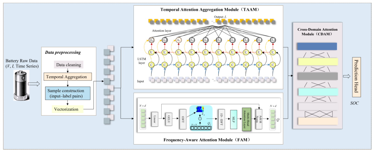
3.1. Overall Framework

The overall architecture of JTFCD-Net is illustrated in Figure 1. The framework consists of four sequential representation-learning stages and two prediction heads. First, a temporal aggregation block extracts multi-scale local temporal patterns from the raw sequence and projects heterogeneous battery measurements into a unified latent space. Second, the Temporal Attention Aggregation Module (TAAM) models long-range dependencies among time steps so that historical operating responses can influence the current-state representation. Third, the Frequency-Aware Attention Module (FAM) transforms the temporal feature into a frequency-aware counterpart by using spectral statistics to recalibrate channels associated with short-window voltage trend variations, transient polarization-related fluctuations, and measurement disturbances. By returning this counterpart to the same feature shape, the model constructs a representation-level temporal–frequency symmetric pair: both views come from the same window and keep matched temporal resolution and hidden width. Fourth, CDAM performs bidirectional cross-attention fusion, allowing the two branches to exchange complementary information rather than being fused by simple concatenation alone. Finally, the fused latent feature is decoded by a main SOC regression head and an auxiliary voltage reconstruction head. Compared with a single-task SOC regressor, this dual-task design improves the reliability of SOC estimation by encouraging the shared representation to retain both state-discriminative information and informative voltage evolution characteristics. Reconstructing the full voltage window provides additional supervision that complements the scalar SOC label and helps the backbone preserve latent dynamics favorable for reliable SOC prediction.
The feature propagation of the proposed model can be summarized as
H ( 0 ) = TA ( X k ) , H ( t ) = TAAM ( H ( 0 ) ) , H ( f ) = FAM ( H ( t ) ) ,
H ( c ) = CDAM ( H ( t ) , H ( f ) ) ,
where  H ( 0 ) , H ( t ) , H ( f ) , H ( c ) R L × d  and d denotes the hidden feature dimension. Therefore, all intermediate modules preserve the temporal resolution L and output features with the same hidden width d, which makes the residual additions and the subsequent multi-task decoding dimensionally valid. The final outputs are a scalar SOC estimate  s ^ k R  and a reconstructed voltage trajectory  v ^ k R L .

3.2. Temporal Aggregation

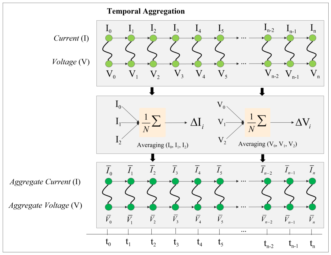
As shown in Figure 2, the temporal aggregation block is used to capture short-term transients and medium-range operating dynamics before applying global attention. This stage is motivated by the fact that battery measurements contain dynamics at multiple temporal scales: abrupt current excitation induces local voltage fluctuation, relaxation effects develop over a longer horizon, and thermal responses usually evolve more smoothly. Instead of relying on a single receptive field, the input sequence is processed by M parallel one-dimensional convolution branches with different kernel sizes  { k 1 , k 2 , , k M } . The output of the m-th branch is defined as
H m = ϕ BN Conv 1 D k m ( X k ; Θ m ) R L × d m , m = 1 , 2 , , M ,
where  Θ m  denotes the learnable parameters of the m-th convolution branch,  ϕ ( · )  is a nonlinear activation function, and  BN ( · )  denotes batch normalization. Zero-padding is adopted so that the temporal length remains L for every branch. The branch dimensions satisfy  m = 1 M d m = d .
The branch outputs are concatenated and combined with a linear projection of the raw input to form the initial hidden feature:
X ˜ k = X k W e R L × d ,
H ( 0 ) = Concat ( H 1 , H 2 , , H M ) + X ˜ k ,
where  W e R d 0 × d  is a learnable embedding matrix. Since  Concat ( H 1 , , H M ) R L × d  by construction, the residual summation with  X ˜ k R L × d  is well defined. Through this design, local current perturbations, voltage relaxation behavior, and temperature-dependent fluctuations are encoded at multiple temporal scales while preserving the original sequence length. In this sense, the temporal aggregation block acts as a structured front end that prepares the sequence for subsequent global dependency modeling.

3.3. Temporal Attention Aggregation Module

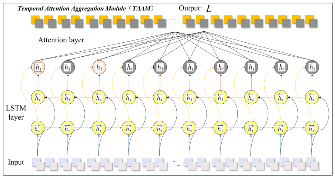
After local temporal encoding, the Temporal Attention Aggregation Module (TAAM) is employed to model long-range dependencies across the entire observation window, as illustrated in Figure 3. The key idea is to move beyond purely local convolutional perception and explicitly associate early-stage operating conditions with later-stage voltage and SOC evolution. Let the number of attention heads be h, and define the per-head dimension as  d h = d / h . For the i-th attention head, the query, key, and value matrices are computed by
Q i = H ( 0 ) W i Q , K i = H ( 0 ) W i K , V i = H ( 0 ) W i V ,
where  Q i , K i , V i R L × d h  and  W i Q , W i K , W i V R d × d h .
The corresponding temporal attention matrix is
A i = softmax Q i K i d h R L × L ,
where the softmax operation is applied row-wise. Hence, every row of  A i  forms a normalized dependency distribution over all time steps in the current observation window. The i-th head output is then given by
head i = A i V i R L × d h .
After concatenating all heads, a residual attention feature is obtained as
H ( a ) = LN Concat ( head 1 , , head h ) W O + H ( 0 ) ,
where  W O R d × d  and  H ( a ) R L × d . Because  Concat ( head 1 , , head h ) R L × d , the residual addition with  H ( 0 )  is dimensionally consistent. The temporal feature is further refined by a position-wise feed-forward network:
FFN ( Z ) = δ ( Z W 1 + b 1 ) W 2 + b 2 ,
W 1 R d × d ff , W 2 R d ff × d ,
H ( t ) = LN FFN ( H ( a ) ) + H ( a ) R L × d .
By explicitly learning the interactions among distant time steps, TAAM improves robustness under highly dynamic charge–discharge conditions where instantaneous observations alone are insufficient for accurate SOC inference. This is especially important when similar terminal voltages may correspond to different latent SOC states under different load histories.

3.4. Frequency-Aware Attention Module

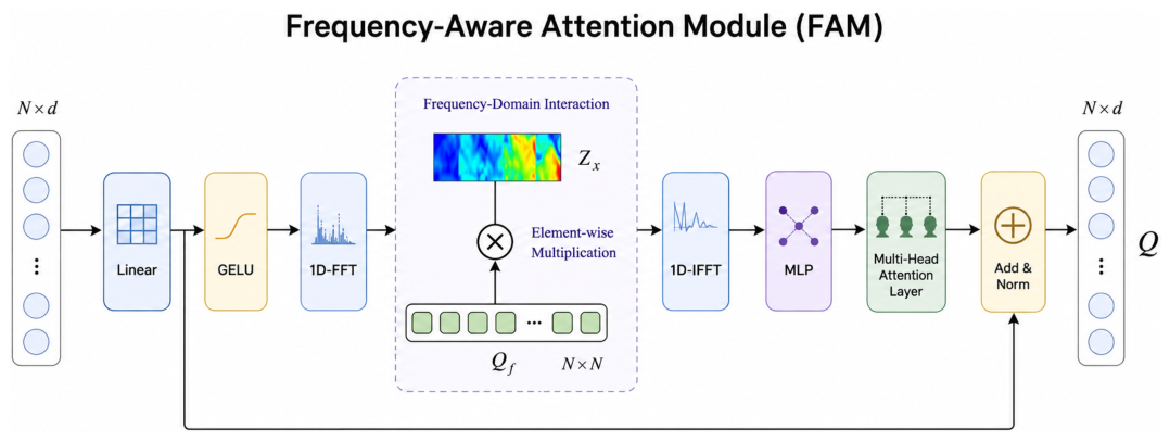
FAM constructs the frequency-aware side of the representation-level symmetry. It should be noted that FAM is not designed as a fine-grained frequency-bin attention mechanism. Instead, it is a lightweight frequency-domain channel recalibration module based on global spectral statistics. Although this design sacrifices explicit frequency-band resolution, it provides a compact way to inject coarse spectral information into the latent temporal representation. With the default window length of  L = 128 , the DFT is applied only within a short sliding window and is not expected to resolve true long-term open-circuit-voltage drift or long-term relaxation time constants. It does not claim a strict time–frequency physical duality. It also does not concatenate handcrafted spectral descriptors to the input. Instead, a single global Fourier transform is applied to the complete sequence, the magnitude spectrum is averaged along the frequency axis, and a two-layer MLP generates channel gates. Within this short window, lower-frequency bins mainly provide coarse local trend information, whereas higher-frequency bins are more related to load-induced transient polarization and measurement disturbance. This design reduces computational cost and improves embedded deployment feasibility, as illustrated in Figure 4.
The temporal feature is first transformed into the frequency domain along the temporal axis:
F = F τ H ( t ) C L × d ,
where  F τ ( · )  denotes the discrete Fourier transform applied over the length-L dimension. A compact channel descriptor is then obtained from the spectral magnitude, where  | · |  denotes element-wise complex modulus:
z f = 1 L = 1 L F , : = 1 L = 1 L | F , 1 | , 1 L = 1 L | F , 2 | , , 1 L = 1 L | F , d | R d .
Therefore, each element of  z f  is the mean spectral magnitude of one latent channel over all frequency bins. FAM is conceptually related to channel recalibration mechanisms such as squeeze-and-excitation, but the channel descriptor in FAM is computed from the spectral magnitude of latent temporal features rather than from ordinary time-domain pooling. Therefore, its role is to perform frequency-aware channel recalibration at the representation level, rather than to serve as a fine-grained physical frequency decomposition module. Based on this descriptor, FAM generates a channel reweighting gate
g f = σ W f , 2 δ W f , 1 z f R d ,
where  δ ( · )  and  σ ( · )  denote the ReLU and sigmoid functions, respectively,  W f , 1 R r × d  and  W f , 2 R d × r  with hidden reduction dimension r. Because  z f  is obtained by averaging over the frequency axis, the resulting gate modulates latent channels rather than assigning separate weights to individual frequency bins.
The gate is broadcast to all frequency bins and used to modulate the complex spectral representation:
A f = 1 L g f R L × d ,
F ^ = F A f C L × d ,
where ⊙ denotes element-wise multiplication and  1 L R L  is an all-ones vector. Because  A f  has the same shape as  F  after broadcasting, the modulation is dimensionally valid for every temporal–frequency element. The frequency-informed temporal representation is then reconstructed by the inverse Fourier transform:
H ( f ) = F τ 1 F ^ R L × d .
This mechanism allows the network to use coarse spectral statistics to recalibrate channels responsive to short-window SOC-related response patterns while suppressing less useful oscillatory content. Since the reconstructed feature returns to the same shape, it forms the frequency-aware counterpart of the temporal representation without additional reshaping.

3.5. Cross-Domain Attention Module

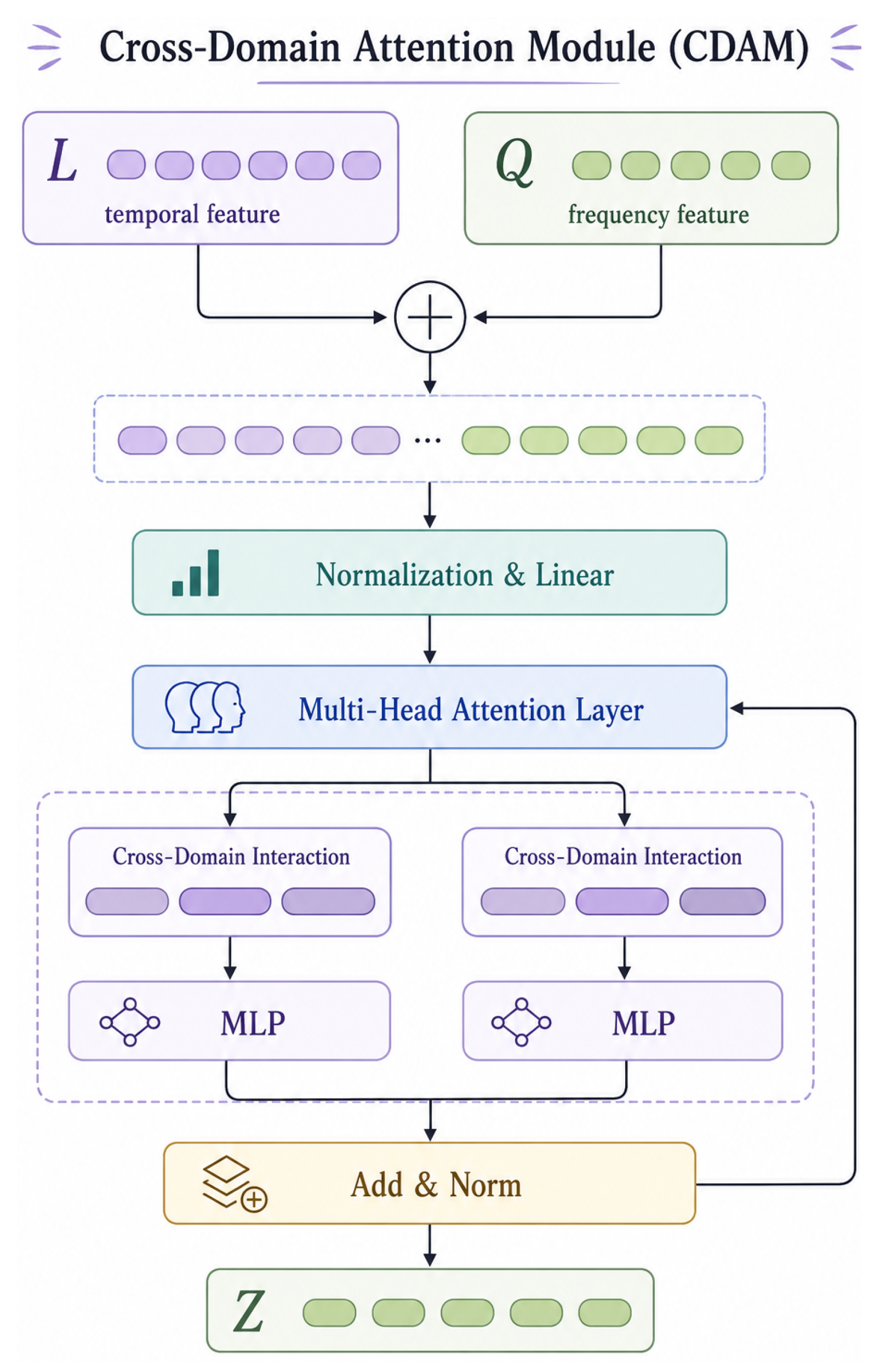
To operationalize representation-level temporal–frequency symmetry, CDAM is adopted for feature interaction, as illustrated in Figure 5. CDAM performs bidirectional cross-attention so that temporal features can query frequency-aware features and vice versa. Thus, symmetry is realized as reciprocal information exchange between two same-shaped representations, not as a reversible transform. Let  d c  denote the shared attention subspace dimension. The frequency-to-temporal attention matrix is defined as
A t f = softmax ( H ( t ) W t Q ) ( H ( f ) W f K ) d c R L × L ,
and the corresponding cross-domain feature is
Z t f = A t f ( H ( f ) W f V ) R L × d c ,
where  W t Q R d × d c  and  W f K , W f V R d × d c .
Similarly, the temporal-to-frequency attention matrix is
A f t = softmax ( H ( f ) W f Q ) ( H ( t ) W t K ) d c R L × L ,
and the corresponding fused feature is
Z f t = A f t ( H ( t ) W t V ) R L × d c ,
where  W f Q R d × d c  and  W t K , W t V R d × d c . The two cross-domain features are concatenated and projected back to the hidden space:
H ( c ) = LN Concat ( Z t f , Z f t ) W c + H ( t ) + H ( f ) R L × d ,
where  W c R 2 d c × d . Since  Concat ( Z t f , Z f t ) R L × 2 d c , the projection through  W c  returns the fusion result to  R L × d , making residual addition with  H ( t )  and  H ( f )  valid. This bidirectional mechanism encourages temporal trajectories and spectral descriptors to calibrate each other, improving representational stability under load changes and operating-condition shifts.
Because CDAM computes two reciprocal  L × L  attention matrices, its cost is higher than simple concatenation. The attention score and value products cost approximately  O ( 4 L 2 d c ) , while the linear projections cost  O ( 8 L d d c ) ; thus, the total cost is  O ( 4 L 2 d c + 8 L d d c )  and the attention-memory cost is  O ( 2 L 2 ) . Since CDAM is applied to fixed-length sliding windows, this cost is controlled by the chosen window length, but it should still be viewed as an accuracy–complexity trade-off. Therefore, CDAM should be interpreted as an explicit temporal–frequency interaction module rather than a low-cost fusion layer. Its benefit must be balanced against the additional matrix multiplication overhead, especially when real-time BMS inference is considered.

3.6. Dual-Task Prediction Heads and Objective Function

Based on the fused feature  H ( c ) , the network performs SOC regression and voltage reconstruction jointly. First, an attention pooling operator is used to obtain a compact sequence representation that emphasizes the most informative time steps for SOC estimation:
α k = softmax H ( c ) w p R L ,
h k = t = 1 L α k , t H t , : ( c ) R d ,
where  w p R d  and  t = 1 L α k , t = 1 . Since  H ( c ) w p  generates an L-dimensional score vector, the temporal softmax naturally assigns a normalized importance weight to each time step in the observation window. The SOC estimate is then produced by
s ^ k = w s h k + b s ,
where  s ^ k R  denotes the predicted SOC at time step k.
For the auxiliary voltage reconstruction task, a time-distributed linear decoder is applied to each hidden state:
v ^ k = squeeze H ( c ) W v + b v R L ,
where  W v R d × 1 . Since  H ( c ) R L × d , the product  H ( c ) W v  yields an output in  R L × 1 , and the squeeze operation removes the singleton channel dimension to obtain a voltage vector of length L. The reconstructed voltage trajectory is compared with the ground-truth voltage sequence
v k = [ V k L + 1 , V k L + 2 , , V k ] R L .
The SOC loss and voltage reconstruction loss are defined as
L SOC = 1 N k = 1 N s ^ k s k 2 ,
L V = 1 N L k = 1 N v ^ k v k 2 2 ,
where N is the number of windowed training samples and  s k  is the Coulomb-counting-based reference SOC label. The overall training objective is
L = L SOC + λ L V ,
where  λ > 0  is a tradeoff coefficient that balances the main SOC task and the auxiliary reconstruction task. The auxiliary voltage reconstruction branch is introduced to improve the reliability of SOC estimation rather than to serve as an independent prediction goal. Although the input window already contains voltage measurements, the reconstruction target is imposed only after the common temporal–frequency backbone and fusion modules, without any direct shortcut from input voltage to the decoder. Therefore, the voltage branch is not intended to copy the raw input voltage or to act as an independent autoencoder. Instead, it regularizes the shared SOC-oriented representation by requiring the fused latent features to preserve voltage-response morphology after multiple nonlinear temporal, spectral, and cross-domain transformations. As a result, the model is encouraged to preserve voltage-response morphology in the shared latent state while still organizing the representation around the main SOC target. From an information-preservation viewpoint, full-window voltage reconstruction helps retain dense observable response information, including ohmic drop, polarization, relaxation, and load-history effects. Since SOC provides only a scalar terminal label for each window, this dense sequence-level target offers a more continuous constraint on intermediate latent states. From an optimization viewpoint, it regularizes the shared backbone and reduces overfitting to sparse terminal SOC labels. This auxiliary constraint also discourages the backbone from learning shortcut features that fit SOC labels but ignore voltage-response dynamics. Therefore, voltage reconstruction provides complementary dense supervision for learning a more informative representation, rather than replacing SOC supervision.

4. Experiments

4.1. Datasets and Data Preparation

Experiments are conducted on the public CALCE A123 battery dataset, as introduced in Ref. [44]. This dataset has been widely adopted in battery modeling and SOC estimation studies because it provides carefully curated cycling records with synchronized voltage, current, and temperature measurements, together with dynamic load profiles that are close to electric-vehicle operating scenarios [45]. In the present work, CALCE is used to evaluate estimation accuracy under different fixed ambient temperatures and operating conditions within a consistent dynamic-drive-cycle setting.
For the CALCE benchmark, this study focuses on the A123 lithium-ion cells tested under dynamic driving-related current profiles. The CALCE dynamic dataset contains three representative operating conditions, namely the Federal Urban Driving Schedule (FUDS), Dynamic Stress Test (DST), and US06 highway driving profile [44]. Among them, FUDS is selected as the primary operating condition for the main comparison experiments. The reason is twofold. First, FUDS describes typical urban electric-vehicle driving behavior, including start-up, acceleration, cruising, deceleration, and stop phases, and is therefore more representative of practical battery-management scenarios than a purely simplified laboratory load. Second, compared with DST, which is derived from a simplified power–time profile, and US06, which emphasizes more aggressive high-speed and high-acceleration operation, FUDS provides a better balance between dynamic richness and practical relevance. Unless otherwise specified, the main experimental setting in this paper is the CALCE A123 dataset under the FUDS profile at 25 °C. In addition, performance under different fixed ambient temperatures is evaluated under 0 °C, 10 °C, 25 °C, and 40 °C, while DST and US06 are retained as supplementary operating conditions for condition-wise comparison.
To examine whether the proposed framework generalizes beyond the original CALCE A123 benchmark, external validation is conducted on the NASA Ames lithium-ion battery aging dataset [46]. Four commonly used laboratory-scale 18650 cells, B0005, B0006, B0007, and B0018, are selected because they provide synchronized voltage, current, measured cell temperature, time, and discharge-capacity records over repeated cycling. In the NASA experiment, SOC labels are generated from the discharge trajectories by the same Coulomb-counting protocol, and a leave-one-cell-out strategy is adopted: one cell is used only for testing, while the remaining three cells are used for training and validation. This protocol evaluates cell-level generalization under an independent public benchmark rather than random sample-level interpolation within a single cell. The NASA dataset is used here as a classical external benchmark and should not be interpreted as a modern high-capacity NMC/NCA EV-pack dataset.
To ensure consistency with the proposed JTFCD-Net, raw measurements are processed under a unified pipeline. First, only complete discharge trajectories containing valid voltage, current, and temperature measurements are retained. Since the present work focuses on SOC estimation together with voltage reconstruction during dynamic evolution, sliding windows are sampled from these discharge trajectories for training and testing. For the main comparative experiments, FUDS discharge trajectories at the selected temperatures are used; DST and US06 are included in the operating-condition study. Second, duplicated timestamps, missing samples, and obvious outliers are removed, after which the remaining trajectories are resampled to a uniform time interval  Δ t  using linear interpolation. This step is necessary because both the dual-task learning target and the temporal modules in JTFCD-Net assume a consistent temporal grid.
The reference SOC labels are generated by Coulomb counting. Let  I t ( d ) 0  denote the discharge current magnitude at time step t and  Q ref  denote the reference capacity used for label construction. The discrete reference SOC label is computed as
s t = s t 1 η I t ( d ) Δ t Q ref ,
where  η  is the Coulombic efficiency and the initial SOC of each selected discharge trajectory is set to  s t 0 = 1 . In the present CALCE study, a unified  Q ref  and constant  η  are adopted for all selected trajectories to keep the label construction protocol consistent across the dataset and all compared models. Therefore, these SOC values are treated as Coulomb-counting-based reference labels rather than error-free physical ground truths.
After label generation, each time step is represented by a multivariate feature vector
x t = [ V t , I t ( d ) , T t , Δ V t , Δ I t ] R 5 ,
where
Δ V t = V t V t 1 , Δ I t = I t ( d ) I t 1 ( d ) .
The inclusion of both raw measurements and first-order temporal differences is designed to match the temporal aggregation block introduced in Section 3.2. Specifically, the multi-branch one-dimensional convolutions in the temporal aggregation module are intended to capture local transients at different receptive fields. The raw channels provide absolute operating-state information, whereas the differential channels explicitly highlight local voltage and current transitions, enabling the convolution branches to respond more effectively to abrupt load perturbations, relaxation behavior, and local trend changes. It should also be noted that first-order differencing may amplify measurement noise, especially under real dynamic driving conditions with imperfect onboard sensors. In this study, this risk is partly mitigated by removing missing samples and obvious outliers, resampling all trajectories to a uniform time grid, normalizing each feature channel using training-set statistics, and processing the resulting features through fixed-length sliding windows with multi-scale convolution and attention-based aggregation. Nevertheless, these operations should be viewed as noise-mitigation measures rather than a complete solution to sensor-noise robustness.
All feature channels are normalized using statistics computed from the training set only:
x ˜ t , j = x t , j μ j σ j ,
where  μ j  and  σ j  denote the mean and standard deviation of the j-th feature channel. Sliding windows are then constructed to form the model input:
X k = [ x ˜ k L + 1 , x ˜ k L + 2 , , x ˜ k ] R L × d 0 ,
where  d 0 = 5  in the present implementation. For each input window, the supervision signals are the terminal SOC label  s k  and the voltage reconstruction target
v k = [ V k L + 1 , V k L + 2 , , V k ] R L .
In this manner, the dataset construction process is fully aligned with the dual-task design of JTFCD-Net. The fixed-length input tensor preserves the local neighborhoods required by temporal aggregation, while the full window voltage target supplies the sequence-level supervision used by the reconstruction branch. This auxiliary target is important because SOC supervision alone is sparse at the window level, whereas reconstructing  v k  encourages the shared backbone to preserve the temporal morphology of battery response, including transient drops, recovery effects, and temperature-dependent polarization behavior. In this paper, the role of the voltage branch is to improve the reliability of SOC estimation by helping the backbone retain informative intermediate dynamics that would otherwise be compressed away when optimizing only the terminal SOC target.
To avoid information leakage, the trajectories of each battery cell are divided in chronological order with a ratio of 70% for training, 15% for validation, and 15% for testing. The earlier portion is used for training, the middle portion for validation, and the later portion for testing, so that the model is always evaluated on later operating stages that are unseen during optimization. All sliding windows inherit the split of the parent trajectory.

4.2. Evaluation Metrics

Since the proposed framework performs both SOC estimation and voltage reconstruction, two groups of evaluation metrics are adopted. For SOC estimation, mean absolute error (MAE), root mean square error (RMSE), and maximum absolute error (MaxE) are used:
MAE SOC = 1 N k = 1 N s ^ k s k ,
RMSE SOC = 1 N k = 1 N s ^ k s k 2 ,
MaxE SOC = max 1 k N s ^ k s k .
Among these metrics, MAE measures average estimation deviation, RMSE penalizes large errors more strongly, and MaxE reflects the worst-case estimation behavior, which is important for battery management applications with safety constraints.
For the auxiliary voltage reconstruction task, mean absolute error and root mean square error are computed over all points in all windows:
MAE V = 1 N L k = 1 N v ^ k v k 1 ,
RMSE V = 1 N L k = 1 N v ^ k v k 2 2 .
The voltage metrics are not only used to assess reconstruction fidelity, but also to verify whether the latent representation learned by JTFCD-Net preserves physically meaningful dynamic information correlated with SOC evolution.

4.3. Experimental Settings

The proposed JTFCD-Net is implemented in PyTorch 2.0.1 and trained end-to-end on a single GPU platform. Unless otherwise stated, the window length is set to  L = 128 , the hidden feature dimension is set to  d = 128 , the number of attention heads in TAAM is  h = 4 , and the shared cross-domain attention dimension in CDAM is set to  d c = 64 . In the temporal aggregation block, three parallel one-dimensional convolution branches are employed with kernel sizes  { 3 , 5 , 7 }  to capture local battery dynamics at different temporal scales. For the feed-forward block in TAAM, the intermediate dimension is set to  d ff = 256 . In FAM, the channel reduction dimension is set to  r = 32 . The loss balancing coefficient in the joint objective is fixed to  λ = 0.2 .
During training, the Adam optimizer is adopted with an initial learning rate of  10 3 , a batch size of 128, and a weight decay of  10 5 . The model is trained for at most 200 epochs, and early stopping is applied according to the validation RMSE to avoid overfitting. The learning rate is reduced automatically when the validation performance saturates. All input normalization statistics are computed only from the training split, and the same normalization parameters are reused for validation and test samples to ensure a fair evaluation protocol.
All compared methods use the same data split and the same input variables whenever possible. The optimizer family, epoch budget, early-stopping criterion, and normalization protocol are kept consistent across methods. This setting helps ensure that the reported performance differences mainly reflect differences in representation learning and supervision design rather than inconsistencies in data partitioning or preprocessing. Under this protocol, the proposed JTFCD-Net can be evaluated consistently on CALCE while maintaining alignment between the dataset construction procedure and the architecture described in Section 3.

4.4. Computational Complexity and Inference Cost

The computational cost of JTFCD-Net is mainly determined by the multi-scale temporal aggregation block, TAAM, FAM, and CDAM. For a window length L, input dimension  d 0 , hidden dimension d, feed-forward dimension  d ff , CDAM projection dimension  d c , and FAM reduction dimension r, the temporal aggregation block costs approximately  O ( L d 0 m = 1 M k m d m + L d 0 d ) . TAAM costs  O ( 4 L d 2 + 2 L 2 d + 2 L d d ff ) , where the  L 2  term comes from temporal self-attention. FAM costs  O ( d L log L + L d + 2 d r )  because it uses one global Fourier transform and a small channel MLP. CDAM costs  O ( 4 L 2 d c + 8 L d d c )  and stores two  L × L  attention matrices. Therefore, TAAM and CDAM dominate the total complexity, while FAM contributes only a small additional cost.
Under the default setting used in this study ( L = 128 d = 128 d ff = 256 d c = 64 , and  r = 32 ), the implemented JTFCD-Net contains approximately  2.4 × 10 5  trainable parameters (0.24 M). Single-window inference was profiled with batch size 1 and  L = 128  on the CPU of the same workstation used for experiments, giving an average latency of about  8.1  ms per window. This result provides a practical reference for the implemented model size and workstation-level inference cost.

4.5. Baseline Models

To verify the effectiveness of the proposed backbone, JTFCD-Net is compared with six representative sequence modeling baselines, including a vanilla recurrent neural network (RNN), LSTM, BiLSTM, 1D-CNN, Transformer, and Mamba. These baselines cover the main families of sequence processing methods that are widely used in time-series learning and battery state estimation, namely plain recurrent modeling [40,47], gated recurrence [17,48], bidirectional recurrence [23,49], convolutional sequence encoding [21,50], self-attention [31,51], and state-space sequence modeling [52]. The inclusion of these methods allows the comparison to cover both classical and recent long-sequence architectures under a unified SOC estimation protocol.
For fairness, all baseline models use the same sliding-window input, the same normalized feature channels, the same train–validation–test split, and the same optimizer family and training schedule described in Section 4.3. The hidden width and number of layers of each baseline are adjusted so that the trainable parameter budgets are kept in the same sub-million scale as JTFCD-Net. The parameter counts reported in Table 1 are rounded implementation-level estimates, including the prediction head, and are used only to indicate model-scale comparability rather than exact framework-independent constants. Unless otherwise stated, recurrent baselines use the final hidden state for SOC regression, whereas 1D-CNN, Transformer, and Mamba apply temporal average pooling followed by the same two-layer multilayer perceptron prediction head. The references associated with each baseline are intended to indicate the original or representative source of the corresponding model family; the baselines used here are standardized implementations under a unified protocol rather than exact reproductions of every published training protocol.
CNN–LSTM [19], a representative hybrid architecture that combines local convolutional feature extraction with recurrent temporal modeling, is included in the main CALCE benchmark. In the NASA external validation, JTFCD-Net is compared with Mamba, which is the strongest baseline in the CALCE experiments, and CNN–LSTM as a hybrid baseline. A full physics-informed-neural-network comparison is not included in the current experimental scope because such models typically require additional physical assumptions, equivalent-circuit identification, or electrochemical parameters that are not uniformly specified in the selected public datasets.

4.6. Comparison with Baseline Methods

Based on the above settings, several groups of comparative experiments are conducted. Unless otherwise specified, the main comparison setting is the CALCE A123 dataset under the FUDS operating profile at 25 °C. On top of this main benchmark, analyses are performed to study performance under different fixed ambient temperatures for FUDS and operating-condition robustness under DST and US06. Following common practice in the battery estimation literature, all SOC errors are multiplied by 100 and reported in percentage form. All external baseline methods are trained using SOC supervision only, and JTFCD-Net (SOC-only) is also reported by setting  λ = 0 . The full JTFCD-Net is trained with the joint SOC estimation and voltage reconstruction objective described in Section 3. This difference in supervision is intentional: the auxiliary voltage branch is part of the proposed method itself and is introduced to improve the reliability of SOC estimation under dynamic conditions. Therefore, the comparison should be interpreted as an overall framework comparison under matched data splits, inputs, and model scale, rather than as a same-supervision ablation of backbone architectures. In all tables, the model names are followed by their representative source references. The architecture ablation studies are conducted under the main setting of CALCE FUDS at 25 °C, while a temperature-input ablation is included in the NASA external validation. This ablation evaluates the use of measured cell-temperature information, not robustness under prescribed pack-level dynamic thermal profiles.
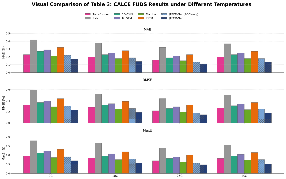
Several observations can be drawn from Table 2, Table 3 and Table 4. First, under the main comparison setting of CALCE FUDS at 25 °C, JTFCD-Net yields the lowest errors, with an MAE of 0.11%, an RMSE of 0.15%, and a MaxE of 0.47%. The CNN–LSTM baseline obtains an RMSE of 0.24%, which is better than the standalone LSTM and 1D-CNN baselines but still weaker than the stronger global-sequence baselines and the proposed method. The SOC-only variant still outperforms the strongest external baseline, while full voltage reconstruction further reduces the RMSE from 0.18% to 0.15%. The improvement over Mamba and Transformer is clear but still moderate, which better reflects a realistic advantage under a strong baseline setting rather than an excessively optimistic gap. Compared with Mamba, the absolute MAE reduction is only 0.04 percentage points, so the engineering impact should be interpreted as incremental rather than decisive.
Second, the CALCE FUDS fixed-temperature comparison results show a clear thermal effect. The most challenging case is 0 °C, where all models exhibit their largest errors. This behavior is physically reasonable because low temperature increases polarization, internal resistance, and voltage hysteresis, making the mapping from measurable terminal signals to latent SOC more nonlinear and less stable. As the temperature approaches 25 °C, the error of every method decreases, which indicates that the electrochemical response becomes easier to model under moderate thermal conditions. At 40 °C, the error rises slightly again, reflecting the influence of temperature-induced side reactions and drift in dynamic behavior. The SOC-only variant is not consistently better than Mamba under all temperatures, whereas the full model remains clearly better after adding voltage reconstruction supervision. However, these controlled isothermal tests should not be interpreted as direct evidence of robustness under continuously varying pack-temperature trajectories during real vehicle operation.
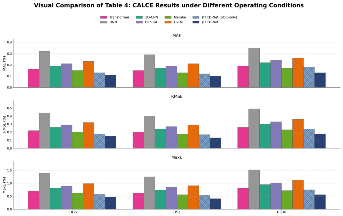
Third, the supplementary CALCE condition comparison demonstrates that the proposed method is not limited to FUDS alone. At 25 °C, JTFCD-Net attains the lowest MAE, RMSE, and MaxE under FUDS, DST, and US06. Among the three conditions, DST is slightly easier because its load profile is more regular, whereas US06 is the most challenging because it contains more aggressive high-power transients. Under US06, JTFCD-Net (SOC-only) is slightly weaker than Mamba, indicating that the auxiliary task is especially useful under aggressive load variation. This pattern is consistent with the design motivation of the temporal and frequency branches: multi-scale local aggregation helps capture rapid current changes, while TAAM, FAM, and CDAM help maintain stable estimation under more abrupt and spectrally complex load profiles.
Fourth, the relative ranking of the baseline models is also informative. The gated recurrent baselines outperform the vanilla RNN, confirming that long-term memory is essential for battery SOC tracking. The 1D-CNN baseline further improves over recurrent models because local transients and short-term voltage-current interactions are important in dynamic SOC estimation. Transformer and Mamba provide stronger performance than the purely recurrent and convolutional baselines, indicating that global dependency modeling is beneficial. Nevertheless, their improvements remain limited compared with JTFCD-Net because they do not explicitly combine multi-scale temporal aggregation, frequency-informed channel recalibration, and cross-domain fusion under a dual-task learning objective.
For clearer interpretation of the numerical results, the data reported in Table 3 and Table 4 are further visualized in grouped bar charts, as shown in Figure 6 and Figure 7. The visual comparison makes the relative margin among competing methods more intuitive. In particular, the advantage of JTFCD-Net can be observed consistently across all three error metrics, and the margin becomes more pronounced under low-temperature or highly dynamic conditions. This performance pattern is consistent with representation-level temporal–frequency symmetry, which incorporates complementary frequency-aware cues into temporal representations.

4.7. External Validation on the NASA Battery Dataset

To further evaluate cell-level generalization, Table 5 reports the leave-one-cell-out results on the NASA battery aging dataset. Three representative methods are included in this external comparison: Mamba as the strongest baseline in the CALCE experiments, CNN–LSTM as a hybrid convolutional–recurrent baseline, and the proposed JTFCD-Net. This focused comparison examines whether the proposed framework remains effective on an independent laboratory-scale public dataset, while broader cross-study comparisons on NASA-based SOC estimation remain outside the scope of this work.
The NASA results show that JTFCD-Net maintains the lowest error when the test cell is excluded from training. Compared with CNN–LSTM, the proposed method reduces the average RMSE from 1.01% to 0.70%. Compared with Mamba, the average RMSE decreases from 0.91% to 0.70%. These results suggest that the proposed representation-level temporal–frequency framework is not only effective under the original CALCE A123 setting, but also provides improved cell-level generalization on a classical external benchmark. Because NASA is not a contemporary high-capacity NMC/NCA EV-pack dataset, this result should be interpreted as reducing single-dataset dependence rather than proving direct EV-pack deployment relevance.
Table 6 further examines the role of measured cell temperature. Removing the temperature channel increases the average RMSE from 0.70% to 0.82%, indicating that the proposed model can exploit measured thermal-response information during cycling. It should be noted that the NASA dataset is still a laboratory-scale cell dataset rather than a full battery-pack dataset with prescribed continuously varying ambient-temperature profiles or spatial pack-level thermal gradients. Therefore, this ablation supports the usefulness of cell-temperature measurements, while full pack-level validation under real vehicle thermal dynamics remains a future direction.

4.8. Voltage Reconstruction Performance

To further validate the effectiveness of the auxiliary branch, Table 7 reports the voltage reconstruction accuracy of JTFCD-Net under the main evaluation settings. Since the baseline models are configured as single-task SOC estimators, they do not contain a sequence-level voltage decoder and are therefore not included in this comparison. The voltage errors are reported in millivolts (mV) for easier physical interpretation.
The voltage reconstruction results show trends that are highly consistent with the SOC estimation results. Reconstruction is most difficult at low temperature and under the aggressive US06 condition, whereas moderate-temperature FUDS and DST settings are easier. This consistency supports the design role of the auxiliary branch: better preservation of voltage-response morphology in the shared representation is associated with more reliable SOC estimation. In other words, voltage reconstruction is introduced to enhance the reliability of the main estimation task rather than to serve as an isolated auxiliary objective.

4.9. Ablation Studies

To analyze the contribution of each design component, a series of ablation experiments are conducted only under the main experimental setting of CALCE FUDS at 25 °C. The ablations focus on five aspects: backbone module contribution, the role of voltage reconstruction supervision, the effect of multi-scale temporal aggregation, the effect of observation window length, and the sensitivity to the loss balancing coefficient. Unless otherwise stated, the ablation experiments follow the same training settings as the full model.
To justify the default choice of  L = 128 , a sensitivity analysis is conducted by changing only the observation window length while keeping the remaining model and training settings unchanged. As shown in Table 8, increasing L from 64 to 128 clearly reduces SOC RMSE, whereas further increasing L to 256 provides only a slight improvement from 0.15% to 0.14%. In contrast, the relative theoretical cost, computed from the complexity terms in Section 4.4 and normalized to  L = 128 , increases to about  2.49 ×  at  L = 256 . Therefore,  L = 128  is selected as a balanced setting between estimation accuracy and computational overhead.
Several conclusions can be drawn from the ablation results. First, Table 9 shows that each proposed module contributes positively to performance under the main benchmark of CALCE FUDS at 25 °C. TAAM provides a substantial improvement over the temporal aggregation front end alone, indicating the importance of long-range dependency modeling. The band-aware FAM variant improves only slightly over TAAM, whereas the proposed FAM yields a larger gain, suggesting that lightweight global spectral channel recalibration is more effective in this setting than explicit band splitting. This ablation compares end-to-end frequency modeling variants within the same backbone, not all handcrafted spectral augmentations. Replacing simple concatenation with CDAM further reduces RMSE from 0.20% to 0.18%, but this improvement is moderate rather than decisive; therefore, CDAM should be viewed as an explicit interaction design whose cost–benefit trade-off requires careful consideration for real-time deployment. The best results are obtained only when all modules are retained and jointly optimized.
Second, Table 10 directly verifies the importance of voltage reconstruction supervision. When the auxiliary branch is removed, the SOC RMSE increases from 0.15% to 0.18%. Replacing full-window voltage reconstruction with only a terminal-voltage target provides limited benefit, but it still remains inferior to reconstructing the entire voltage sequence. This result supports the central design choice of the paper: dense sequence-level voltage supervision helps preserve informative intermediate dynamics and thereby improves the reliability of SOC estimation more effectively than a point-wise auxiliary target.
Third, Table 11 shows that the multi-scale temporal aggregation strategy is consistently better than any single receptive field. This observation is physically intuitive because battery voltage response contains short-term current-induced drops, medium-term polarization effects, and slower recovery components. A single convolution kernel cannot capture all these dynamics equally well, whereas the proposed multi-branch design provides a more complete local description before the sequence is processed by the later attention and cross-domain modules.
Fourth, Table 8 shows that the default window length is a practical compromise. The shorter window  L = 64  reduces cost but loses useful temporal context, while  L = 256  yields only marginal accuracy improvement at substantially higher computational cost.
Finally, Table 12 shows that the tradeoff coefficient  λ  should remain moderate. When  λ  is too small, the auxiliary branch cannot contribute enough reliability-enhancing supervision; when it is too large, the optimization focus shifts excessively toward voltage reconstruction. The best balance is achieved at  λ = 0.2 , which is therefore adopted in all main experiments.

5. Conclusions and Future Work

5.1. Summary of Findings

In this work, we demonstrate that representation-level temporal–frequency symmetry is a promising direction for data-driven battery modeling. By integrating same-space domain representations, reciprocal interaction, and measurement-consistent supervision, the proposed framework provides a more informative description of battery dynamics. Experiments on the CALCE battery dataset showed that the proposed framework maintains strong estimation performance under different fixed ambient temperatures and operating conditions. In particular, under the main benchmark of CALCE FUDS at 25 °C, JTFCD-Net yields the lowest SOC errors among the compared baselines, while the auxiliary voltage reconstruction task contributes directly to improving the reliability of SOC estimation. However, the absolute gain over a strong Mamba baseline is modest, and its direct engineering value for deployed BMS should not be overstated. The NASA validation further shows that JTFCD-Net outperforms the selected comparison methods under a leave-one-cell-out protocol, and the temperature-input ablation confirms the usefulness of measured cell-temperature information. The ablation studies further show that the performance gain is not attributable to a single component alone, but to the combined effect of multi-scale temporal aggregation, temporal attention, frequency-informed channel recalibration, cross-domain fusion, and dense voltage reconstruction supervision.

5.2. Limitations

This study has several limitations. First, the experiments are mainly conducted on the public CALCE dataset under controlled conditions, so the practical value of the observed sub-percentage SOC improvement still requires validation in real onboard BMS scenarios. Second, FAM uses global spectral statistics for channel recalibration and does not explicitly model fine-grained frequency bands or handcrafted spectral-feature augmentation. Third, CDAM introduces quadratic attention cost with respect to the window length, which may limit scalability for much longer observation windows. Although the NASA experiment improves the external validation beyond CALCE, NASA is still a laboratory-scale 18650 cell benchmark rather than a modern high-capacity NMC/NCA EV-pack dataset. Therefore, the claims of this study are limited to cell-level SOC estimation on public laboratory datasets, and future work should further validate the method on contemporary high-capacity EV cells and pack-level data under real driving and thermal conditions. In addition, the reported inference latency is measured on a workstation CPU rather than on a resource-constrained BMS microcontroller. Therefore, the real-time feasibility of direct embedded deployment still requires hardware-specific validation under memory, power, and scheduling constraints. In particular, the performance gain of CDAM over concat fusion is limited relative to its additional attention-matrix computations, so the current design has not yet fully optimized the accuracy–complexity trade-off for real-time SOC estimation. The temperature experiments are also limited to several controlled fixed ambient temperatures. They do not cover continuously varying thermal profiles or spatial temperature gradients in battery packs; therefore, the present results cannot fully demonstrate robustness under realistic dynamic temperature conditions. Another important limitation is that the present experiments evaluate robustness mainly under different fixed ambient temperatures and operating conditions, but do not systematically test SOC estimation under different aging stages or capacity-fade levels. Therefore, the current results should not be interpreted as direct evidence that JTFCD-Net is robust to battery aging, where capacity loss, internal-resistance growth, stronger polarization, and voltage–SOC relationship drift may all affect estimation accuracy. Moreover, the Coulomb-counting labels are generated with a unified reference capacity and constant Coulombic efficiency, so trajectory-level capacity variations caused by temperature, discharge rate, aging, and polarization effects are not explicitly corrected.

5.3. Future Work

Although the present framework has achieved encouraging results, several directions remain worth exploring. First, the current model was evaluated mainly on controlled public datasets, so future work should investigate deployment-oriented validation under onboard battery management scenarios with sensor drift, packet loss, and domain shift across battery chemistries. Such validation is necessary to determine whether the observed sub-percentage error reduction translates into meaningful BMS-level benefit. The NASA validation is a useful external benchmark, but it does not replace validation on modern high-capacity EV cells or pack-level data. Meanwhile, future work will further validate the proposed method on additional public battery datasets, such as Oxford and MIT, to more comprehensively evaluate its generalization ability across different battery types, testing conditions, and aging scenarios. Future tests should also include realistic sensor-noise injection or onboard data collection to evaluate whether the first-order differential channels remain stable under noise amplification. Future work will further use datasets with dynamic temperature trajectories and mixed-temperature operation, and will explore thermal-history modeling or temperature-aware adaptation to improve robustness under realistic thermal variation. In addition, future work will introduce datasets covering different SOH levels, cycle aging stages, capacity-fade degrees, and internal-resistance variations, and will investigate whether SOH estimates, aging descriptors, capacity-fade indicators, or aging-aware physical constraints can improve SOC estimation reliability under aged-battery conditions. Future label construction will also consider trajectory-level capacity calibration, temperature/rate-aware capacity correction, and aging-aware SOH–SOC joint modeling to reduce systematic errors in reference SOC labels. Second, the proposed representation-level temporal–frequency design can be extended with stronger physical constraints, such as equivalent-circuit priors, degradation descriptors, or electrochemical consistency regularization, so that interpretability and extrapolation ability can be improved simultaneously. Future work should also include fair comparisons with physics-informed neural networks or electrochemical-model-guided estimators when the required physical parameters and identification protocols are available. Third, this study focuses on SOC estimation and voltage reconstruction, whereas future research may generalize the framework to multi-state joint estimation, including state-of-health, state-of-power, and remaining useful life estimation. Future work will also investigate finer-grained frequency-band modeling and efficient cross-domain attention variants to improve frequency resolution and scalability. More specifically, lightweight attention, sparse or low-rank interaction, linear attention, and gated fusion mechanisms will be explored to reduce CDAM-related matrix multiplication overhead while preserving useful temporal–frequency exchange. Finally, lightweight model compression and online adaptation strategies should be considered to make the method more practical for real-time embedded battery management systems. Future deployment-oriented work will further profile the model on representative BMS microcontrollers and evaluate quantization, pruning, and efficient-attention replacements under embedded memory and latency constraints.

Author Contributions

Conceptualization, J.L. and X.J.; methodology, J.L.; software, J.L.; validation, J.L. and X.J.; formal analysis, J.L.; investigation, J.L.; data curation, J.L.; writing—original draft preparation, J.L.; writing—review and editing, X.J.; supervision, X.J. All authors have read and agreed to the published version of the manuscript.

Funding

This research received no external funding.

Data Availability Statement

The data used in this study are publicly available from the CALCE Battery Data repository maintained by the Center for Advanced Life Cycle Engineering (CALCE), University of Maryland, at https://calce.umd.edu/battery-data (accessed on 20 March 2026). The NASA battery aging dataset is publicly available from the NASA Ames Prognostics Data Repository at http://ti.arc.nasa.gov/project/prognostic-data-repository (accessed on 3 March 2026).

Conflicts of Interest

The authors declare no conflicts of interest.

References

  1. Xiong, R.; Cao, J.; Yu, Q.; He, H.; Sun, F. Critical review on the battery state of charge estimation methods for electric vehicles. IEEE Access 2017, 6, 1832–1843. [Google Scholar] [CrossRef]
  2. Wang, Y.; Tian, J.; Sun, Z.; Wang, L.; Xu, R.; Li, M.; Chen, Z. A comprehensive review of battery modeling and state estimation approaches for advanced battery management systems. Renew. Sustain. Energy Rev. 2020, 131, 110015. [Google Scholar] [CrossRef]
  3. Demirci, O.; Taskin, S.; Schaltz, E.; Demirci, B.A. Review of battery state estimation methods for electric vehicles-part I: SOC estimation. J. Energy Storage 2024, 87, 111435. [Google Scholar] [CrossRef]
  4. Zheng, Y.; Ouyang, M.; Han, X.; Lu, L.; Li, J. Investigating the error sources of the online state of charge estimation methods for lithium-ion batteries in electric vehicles. J. Power Sources 2018, 377, 161–188. [Google Scholar] [CrossRef]
  5. Wang, S.L.; Fernandez, C.; Cao, W.; Zou, C.Y.; Yu, C.M.; Li, X.X. An adaptive working state iterative calculation method of the power battery by using the improved Kalman filtering algorithm and considering the relaxation effect. J. Power Sources 2019, 428, 67–75. [Google Scholar] [CrossRef]
  6. Zhang, Y.; Li, Y.F. Prognostics and health management of Lithium-ion battery using deep learning methods: A review. Renew. Sustain. Energy Rev. 2022, 161, 112282. [Google Scholar] [CrossRef]
  7. Xing, Y.; He, W.; Pecht, M.; Tsui, K.L. State of charge estimation of lithium-ion batteries using the open-circuit voltage at various ambient temperatures. Appl. Energy 2014, 113, 106–115. [Google Scholar] [CrossRef]
  8. Zheng, F.; Xing, Y.; Jiang, J.; Sun, B.; Kim, J.; Pecht, M. Influence of different open circuit voltage tests on state of charge online estimation for lithium-ion batteries. Appl. Energy 2016, 183, 513–525. [Google Scholar] [CrossRef]
  9. Hossain, M.; Haque, M.E.; Arif, M.T. Kalman filtering techniques for the online model parameters and state of charge estimation of the Li-ion batteries: A comparative analysis. J. Energy Storage 2022, 51, 104174. [Google Scholar] [CrossRef]
  10. Naseri, F.; Schaltz, E.; Stroe, D.I.; Gismero, A.; Farjah, E. An enhanced equivalent circuit model with real-time parameter identification for battery state-of-charge estimation. IEEE Trans. Ind. Electron. 2022, 69, 3743–3751. [Google Scholar] [CrossRef]
  11. Li, W.; Fan, Y.; Ringbeck, F.; Jöst, D.; Han, X.; Ouyang, M.; Sauer, D.U. Electro-chemical model-based state estimation for lithium-ion batteries with adaptive unscented Kalman filter. J. Power Sources 2020, 476, 228534. [Google Scholar] [CrossRef]
  12. Monirul, I.M.; Qiu, L.; Ruby, R. Accurate SOC estimation of ternary lithium-ion batteries by HPPC test-based extended Kalman filter. J. Energy Storage 2024, 92, 112304. [Google Scholar] [CrossRef]
  13. Luo, K.; Chen, X.; Zheng, H.; Shi, Z. A review of deep learning approach to predicting the state of health and state of charge of lithium-ion batteries. J. Energy Chem. 2022, 74, 159–173. [Google Scholar] [CrossRef]
  14. Sesidhar, D.; Badachi, C.; Green, R.C., II. A review on data-driven SOC estimation with Li-Ion batteries: Implementation methods & future aspirations. J. Energy Storage 2023, 72, 108420. [Google Scholar] [CrossRef]
  15. Tian, J.; Chen, C.; Shen, W.; Sun, F.; Xiong, R. Deep learning framework for lithium-ion battery state of charge estimation: Recent advances and future perspectives. Energy Storage Mater. 2023, 61, 102883. [Google Scholar] [CrossRef]
  16. Yang, F.; Li, W.; Li, C.; Miao, Q. State-of-charge estimation of lithium-ion batteries based on gated recurrent neural network. Energy 2019, 175, 66–75. [Google Scholar] [CrossRef]
  17. Yang, F.; Song, X.; Xu, F.; Tsui, K.L. State-of-charge estimation of lithium-ion batteries via long short-term memory network. IEEE Access 2019, 7, 53792–53799. [Google Scholar] [CrossRef]
  18. Li, C.; Xiao, F.; Fan, Y. An approach to state of charge estimation of lithium-ion batteries based on recurrent neural networks with gated recurrent unit. Energies 2019, 12, 1592. [Google Scholar] [CrossRef]
  19. Song, X.; Yang, F.; Wang, D.; Tsui, K.L. Combined CNN-LSTM network for state-of-charge estimation of lithium-ion batteries. IEEE Access 2019, 7, 88894–88902. [Google Scholar] [CrossRef]
  20. Mamo, T.; Wang, F.K. Long short-term memory with attention mechanism for state of charge estimation of lithium-ion batteries. IEEE Access 2020, 8, 94140–94151. [Google Scholar] [CrossRef]
  21. Fan, X.; Zhang, W.; Zhang, C.; Chen, A.; An, F. SOC estimation of Li-ion battery using convolutional neural network with U-Net architecture. Energy 2022, 256, 124612. [Google Scholar] [CrossRef]
  22. Han, Y.; Liu, Y.; Huang, Q.; Zhang, Y. SOC estimation for lithium-ion batteries based on BiGRU with SE attention and Savitzky-Golay filter. J. Energy Storage 2024, 90, 111930. [Google Scholar] [CrossRef]
  23. Sherkatghanad, Z.; Ghazanfari, A.; Makarenkov, V. A self-attention-based CNN-Bi-LSTM model for accurate state-of-charge estimation of lithium-ion batteries. J. Energy Storage 2024, 88, 111524. [Google Scholar] [CrossRef]
  24. Qian, C.; Guan, H.; Xu, B.; Xia, Q.; Sun, B.; Ren, Y.; Wang, Z. A CNN-SAM-LSTM hybrid neural network for multi-state estimation of lithium-ion batteries under dynamical operating conditions. Energy 2024, 294, 130764. [Google Scholar] [CrossRef]
  25. Tian, Y.; Lai, R.; Li, X.; Xiang, L.; Tian, J. A combined method for state-of-charge estimation for lithium-ion batteries using a long short-term memory network and an adaptive cubature Kalman filter. Appl. Energy 2020, 265, 114789. [Google Scholar] [CrossRef]
  26. Chen, J.; Zhang, Y.; Li, W.; Cheng, W.; Zhu, Q. State of charge estimation for lithium-ion batteries using gated recurrent unit recurrent neural network and adaptive Kalman filter. J. Energy Storage 2022, 55, 105396. [Google Scholar] [CrossRef]
  27. Yan, X.; Zhou, G.; Wang, W.; Zhou, P.; He, Z. A hybrid data-driven method for state-of-charge estimation of lithium-ion batteries. IEEE Sens. J. 2022, 22, 16263–16275. [Google Scholar] [CrossRef]
  28. Yu, H.; Lu, H.; Zhang, Z.; Yang, L. A generic fusion framework integrating deep learning and Kalman filter for state of charge estimation of lithium-ion batteries: Analysis and comparison. J. Power Sources 2024, 623, 235493. [Google Scholar] [CrossRef]
  29. Wang, C.; Li, R.; Cao, Y.; Li, M. A hybrid model for state of charge estimation of lithium-ion batteries utilizing improved adaptive extended Kalman filter and long short-term memory neural network. J. Power Sources 2024, 620, 235272. [Google Scholar] [CrossRef]
  30. Hannan, M.A.; How, D.N.T.; Lipu, M.S.H.; Mansor, M.; Ker, P.J.; Dong, Z.Y.; Sahari, K.S.M.; Tiong, S.K.; Muttaqi, K.M.; Mahlia, T.M.I.; et al. Deep learning approach towards accurate state of charge estimation for lithium-ion batteries using self-supervised transformer model. Sci. Rep. 2021, 11, 19541. [Google Scholar] [CrossRef]
  31. Shen, H.; Zhou, X.; Wang, Z.; Wang, J. State of charge estimation for lithium-ion battery using transformer with immersion and invariance adaptive observer. J. Energy Storage 2022, 45, 103768. [Google Scholar] [CrossRef]
  32. Zhao, J.; Han, X.; Wu, Y.; Wang, Z.; Burke, A.F. Opportunities and challenges in transformer neural networks for battery state estimation: Charge, health, lifetime, and safety. J. Energy Chem. 2025, 102, 463–496. [Google Scholar] [CrossRef]
  33. Zou, Y.; Wang, S.; Cao, W.; Hai, N.; Fernandez, C. Enhanced transformer encoder long short-term memory hybrid neural network for multiple temperature state of charge estimation of lithium-ion batteries. J. Power Sources 2025, 632, 236411. [Google Scholar] [CrossRef]
  34. Zhou, Y.; Wang, C.; Gu, T.; Jie, H.; Tao, Z.; Gao, R.X.-K.; See, K.Y.; Zhao, Z. State of charge estimation of lithium-ion batteries using transfer dual-stream physics-informed network. J. Energy Storage 2026, 141, 119451. [Google Scholar] [CrossRef]
  35. Hu, Y.; Huang, D.; Fang, J.; Zhang, C.; Li, H. A joint estimation of state-of-charge and state-of-power for series battery packs based on differential model. J. Energy Storage 2026, 141, 119409. [Google Scholar] [CrossRef]
  36. Wang, J.; Song, J.; Li, Y.; Ren, T.; Yang, Z. State of charge estimation for lithium-ion battery based on improved online parameters identification and adaptive square root unscented Kalman filter. J. Energy Storage 2024, 77, 109977. [Google Scholar] [CrossRef]
  37. Zhu, C.; Wang, S.; Yu, C.; Zhou, H.; Fernandez, C.; Guerrero, J.M. An improved Cauchy robust correction-sage Husa extended Kalman filtering algorithm for high-precision SOC estimation of lithium-ion batteries in new energy vehicles. J. Energy Storage 2024, 88, 111552. [Google Scholar] [CrossRef]
  38. Hannan, M.A.; Lipu, M.S.H.; Hussain, A.; Saad, M.H.; Ayob, A. Neural network approach for estimating state of charge of lithium-ion battery using backtracking search algorithm. IEEE Access 2018, 6, 10069–10079. [Google Scholar] [CrossRef]
  39. Feng, X.; Chen, J.; Zhang, Z.; Miao, S.; Zhu, Q. State-of-charge estimation of lithium-ion battery based on clockwork recurrent neural network. Energy 2021, 236, 121360. [Google Scholar] [CrossRef]
  40. Vidal, C.; Malysz, P.; Naguib, M.; Emadi, A.; Kollmeyer, P.J. Estimating battery state of charge using recurrent and non-recurrent neural networks. J. Energy Storage 2022, 47, 103660. [Google Scholar] [CrossRef]
  41. Wang, S.; Takyi-Aninakwa, P.; Jin, S.; Yu, C.; Fernandez, C.; Stroe, D.I. An improved feedforward-long short-term memory modeling method for the whole-life-cycle state of charge prediction of lithium-ion batteries considering current-voltage-temperature variation. Energy 2022, 254, 124224. [Google Scholar] [CrossRef]
  42. Chen, J.; Zhang, Y.; Wu, J.; Cheng, W.; Zhu, Q. SOC estimation for lithium-ion battery using the LSTM-RNN with extended input and constrained output. Energy 2023, 262, 125375. [Google Scholar] [CrossRef]
  43. Li, F.; Zuo, W.; Zhou, K.; Li, Q.; Huang, Y.; Zhang, G. State-of-charge estimation of lithium-ion battery based on second order resistor-capacitance circuit-PSO-TCN model. Energy 2024, 289, 130025. [Google Scholar] [CrossRef]
  44. Center for Advanced Life Cycle Engineering. Battery Data; University of Maryland: College Park, MD, USA, 2026. [Google Scholar]
  45. Birkl, C.R.; Roberts, M.R.; McTurk, E.; Bruce, P.G.; Howey, D.A. Degradation diagnostics for lithium ion cells. J. Power Sources 2017, 341, 373–386. [Google Scholar] [CrossRef]
  46. Saha, B.; Goebel, K. Battery Data Set; NASA Ames Prognostics Data Repository, NASA Ames Research Center: Moffett Field, CA, USA, 2007.
  47. Elman, J.L. Finding Structure in Time. Cogn. Sci. 1990, 14, 179–211. [Google Scholar] [CrossRef]
  48. Hochreiter, S.; Schmidhuber, J. Long Short-Term Memory. Neural Comput. 1997, 9, 1735–1780. [Google Scholar] [CrossRef] [PubMed]
  49. Schuster, M.; Paliwal, K.K. Bidirectional Recurrent Neural Networks. IEEE Trans. Signal Process. 1997, 45, 2673–2681. [Google Scholar] [CrossRef]
  50. Bai, S.; Kolter, J.Z.; Koltun, V. An Empirical Evaluation of Generic Convolutional and Recurrent Networks for Sequence Modeling. arXiv 2018, arXiv:1803.01271. [Google Scholar] [CrossRef]
  51. Vaswani, A.; Shazeer, N.; Parmar, N.; Uszkoreit, J.; Jones, L.; Gomez, A.N.; Kaiser, Ł.; Polosukhin, I. Attention Is All You Need. In Proceedings of the Advances in Neural Information Processing Systems, Long Beach, CA, USA, 4–9 December 2017; pp. 5998–6008. [Google Scholar]
  52. Gu, A.; Dao, T. Mamba: Linear-Time Sequence Modeling with Selective State Spaces. arXiv 2024, arXiv:2312.00752. [Google Scholar] [CrossRef]
Figure 1. Overall architecture of the proposed JTFCD-Net for joint battery SOC estimation and voltage reconstruction.
Symmetry 18 00931 g001
Figure 2. Structure of the temporal aggregation block, which extracts multi-scale local temporal patterns from battery measurement sequences.
Symmetry 18 00931 g002
Figure 3. Temporal Attention Aggregation module (TAAM), which captures long-range temporal dependencies and adaptively reweights informative time steps.
Symmetry 18 00931 g003
Figure 4. Frequency-Aware Attention Module (FAM), which uses frequency-domain statistics to recalibrate latent channels while preserving the shared representation shape.
Symmetry 18 00931 g004
Figure 5. Cross-Domain Attention Module (CDAM), which enables reciprocal querying between aligned temporal and frequency-aware representations.
Symmetry 18 00931 g005
Figure 6. Grouped bar-chart visualization of the results reported in Table 3, showing the MAE, RMSE, and MaxE comparisons under different fixed ambient temperatures for the CALCE FUDS setting.
Symmetry 18 00931 g006
Figure 7. Grouped bar-chart visualization of the results reported in Table 4, showing the MAE, RMSE, and MaxE comparisons under different operating conditions at 25 °C.
Symmetry 18 00931 g007
Table 1. Backbone configurations of the compared baseline models. All methods are configured with model sizes comparable to JTFCD-Net.
MethodRepresentative ArchitectureConfiguration Used in This WorkApprox. Params (M)
Transformer [51]Encoder-only self-attention2 encoder blocks, d = 128 , h = 4 , d ff = 256 0.23
RNN [47]Vanilla Elman RNN2 recurrent layers, hidden size 1440.19
1D-CNN [50]Temporal convolutional encoder4 Conv1D blocks, channels 64/96/128/128, kernels 7/5/5/30.20
BiLSTM [49]Bidirectional LSTM2 BiLSTM layers, hidden size 72 per direction0.24
CNN–LSTM [19]Hybrid convolutional–recurrent model2 Conv1D blocks, channels 64/128, kernel 5; 2 LSTM layers, hidden size 960.20
Mamba [52]Selective state-space model3 Mamba blocks, d = 128 , state size 160.22
LSTM [48]Gated recurrent network2 LSTM layers, hidden size 960.23
JTFCD-Net (ours)Temporal–frequency cross-domain modelTA + TAAM + FAM + CDAM, d = 128 , h = 4 , d c = 64 0.24
Table 2. Main SOC estimation comparison on the CALCE A123 dataset under the FUDS profile at 25 °C. All values are reported in %. Bold numbers indicate the best performance (lowest error) for each metric.
MethodMAERMSEMaxE
Transformer [51]0.160.220.70
RNN [47]0.320.441.39
1D-CNN [50]0.190.260.82
BiLSTM [49]0.210.290.90
CNN–LSTM [19]0.180.240.76
Mamba [52]0.150.200.62
LSTM [48]0.230.320.99
JTFCD-Net (SOC-only)0.130.180.57
JTFCD-Net (ours)0.110.150.47
Table 3. SOC estimation results on the CALCE A123 dataset under the FUDS profile at different fixed ambient temperatures. All values are reported in %, and lower values indicate better performance. Bold numbers indicate the best performance (lowest error) for each metric.
Method0°C10 °C25 °C40 °C
MAERMSEMaxEMAERMSEMaxEMAERMSEMaxEMAERMSEMaxE
Transformer [51]0.230.320.950.200.280.840.160.220.700.200.270.82
RNN [47]0.420.591.790.380.521.660.320.441.390.370.501.56
1D-CNN [50]0.270.371.120.230.320.960.190.260.820.230.310.95
BiLSTM [49]0.290.401.210.250.351.070.210.290.900.250.341.04
Mamba [52]0.210.290.870.180.250.760.150.200.620.180.240.73
LSTM [48]0.320.441.310.280.391.180.230.320.990.270.371.14
JTFCD-Net (SOC-only)0.220.300.910.190.260.790.130.180.570.180.250.76
JTFCD-Net (ours)0.170.230.700.140.190.580.110.150.470.130.180.53
Table 4. SOC estimation results on the CALCE A123 dataset under different operating conditions at 25 °C. All values are reported in %. Bold numbers indicate the best-performing results (minimum MAE/RMSE/MaxE) across all compared methods for each operating condition.
MethodFUDSDSTUS06
MAERMSEMaxEMAERMSEMaxEMAERMSEMaxE
Transformer [51]0.160.220.700.150.200.630.190.260.81
RNN [47]0.320.441.390.290.401.250.350.491.52
1D-CNN [50]0.190.260.820.170.240.740.220.300.95
BiLSTM [49]0.210.290.900.190.270.840.240.331.02
Mamba [52]0.150.200.620.130.180.560.170.230.72
LSTM [48]0.230.320.990.210.290.910.260.361.12
JTFCD-Net (SOC-only)0.130.180.570.120.170.530.180.240.75
JTFCD-Net (ours)0.110.150.470.100.130.410.130.180.56
Table 5. External SOC estimation validation on the NASA battery aging dataset under the leave-one-cell-out protocol. Cell-specific columns report RMSE, while average values report MAE, RMSE, and MaxE. All values are reported in %. Bold numbers denote the best performance (lowest error) for each metric.
MethodB0005B0006B0007B0018Avg. MAEAvg. RMSEAvg. MaxE
Mamba [52]0.840.960.791.040.680.912.91
CNN–LSTM [19]0.951.070.881.140.751.013.19
JTFCD-Net (ours)0.660.750.610.790.520.702.30
Table 6. Temperature-input ablation on the NASA battery aging dataset. All values are average results over the four leave-one-cell-out test settings and are reported in %. Bold numbers denote the best performance (lowest error) for each metric.
Model SettingAvg. MAEAvg. RMSEAvg. MaxE
JTFCD-Net without temperature input0.610.822.70
JTFCD-Net with temperature input0.520.702.30
Table 7. Voltage reconstruction performance of JTFCD-Net under different CALCE settings. Lower values indicate better reconstruction fidelity.
Condition MAE V (mV) RMSE V (mV)
CALCE FUDS, 0 °C8.912.8
CALCE FUDS, 10 °C7.510.8
CALCE FUDS, 25 °C6.28.6
CALCE FUDS, 40 °C6.99.7
CALCE DST, 25 °C5.88.1
CALCE US06, 25 °C7.911.3
Table 8. Sensitivity analysis of observation window length under the main CALCE FUDS setting at 25 °C. The relative theoretical cost is normalized to the default setting L = 128 . Bold numbers denote the default setting L = 128 selected for the main experiments, which balances estimation accuracy and computational overhead.
Window Length LSOC MAE (%)SOC RMSE (%)Relative Theoretical Cost
640.140.18 0.44 ×
1280.110.15 1.00 ×
2560.100.14 2.49 ×
Table 9. Backbone ablation study of JTFCD-Net under the main setting of CALCE FUDS at 25 °C. Results are reported in %. Bold numbers denote the best performance (lowest error) for each metric.
VariantMAERMSEMaxE
TA only0.270.381.11
TA + TAAM0.200.280.86
TA + TAAM + band-aware FAM0.190.260.81
TA + TAAM + FAM0.170.240.72
TA + TAAM + FAM + concat fusion0.140.200.61
TA + TAAM + FAM + CDAM (without L V )0.130.180.57
Full JTFCD-Net0.110.150.47
Table 10. Ablation study on voltage supervision under the main setting of CALCE FUDS at 25 °C. Results are reported in %, except for voltage RMSE, which is reported in mV. Bold numbers denote the best performance (lowest error) for each metric.
Supervision StrategySOC MAESOC RMSESOC MaxEV RMSE (mV)
SOC only ( λ = 0 )0.130.180.57
SOC + terminal-voltage prediction0.120.170.5314.2
SOC + full-window voltage reconstruction0.110.150.478.6
Table 11. Ablation study on temporal aggregation scale selection under the main setting of CALCE FUDS at 25 °C. Results are reported in %. Bold numbers denote the best performance (lowest error) for each metric.
Temporal Aggregation SettingMAERMSEMaxE
Single-scale kernel { 3 } 0.140.190.58
Single-scale kernel { 5 } 0.130.180.55
Single-scale kernel { 7 } 0.140.190.57
Multi-scale kernels { 3 , 5 , 7 } 0.110.150.47
Table 12. Sensitivity analysis of the loss balancing coefficient λ under the main setting of CALCE FUDS at 25 °C. Bold numbers denote the best performance (lowest error) for each metric.
λ SOC MAE (%)SOC RMSE (%)SOC MaxE (%)V RMSE (mV)
0.00.130.180.57
0.10.120.160.509.4
0.20.110.150.478.6
0.30.110.160.498.8
0.50.120.170.539.5
Disclaimer/Publisher’s Note: The statements, opinions and data contained in all publications are solely those of the individual author(s) and contributor(s) and not of MDPI and/or the editor(s). MDPI and/or the editor(s) disclaim responsibility for any injury to people or property resulting from any ideas, methods, instructions or products referred to in the content.