An Adaptive Multi-Strategy Enhanced Educational Competition Optimizer for Global Optimization and Real-World Problems

Abstract

The Educational Competition Optimizer (ECO) shows promise on simple tasks but struggles with high-dimensional and complex landscapes due to rigid stage division and limited search operators. This paper proposes a Hybrid Strategy Enhanced ECO (HSECO) featuring: (i) a self-adaptive parameter evolution mechanism for individual-level flexibility, (ii) a multi-operator adaptive selection scheme switching between learning and differential evolution strategies based on real-time feedback, and (iii) an archive-assisted diversity preservation module to mitigate premature convergence. HSECO is validated on CEC2017, CEC2020 and CEC2022, and a continuous engineering benchmark. Statistical tests confirm its superiority over nine State-of-the-Art and parameter-free algorithms in accuracy, convergence speed, and robustness. Ablation and diversity analyses verify its balanced exploration–exploitation dynamics. Finally, HSECO is applied to a three-dimensional UAV path-planning problem, where path length, altitude variation, and turning smoothness are integrated into a single fitness function using a weighted-sum formulation. Therefore, from a metaheuristic optimization perspective, the UAV case is treated as a single-objective constrained optimization problem rather than a Pareto-based multi-objective problem. Experimental results show that HSECO obtains shorter, safer, and smoother trajectories with lower overall weighted fitness.

1. Introduction

With the continuous increase in engineering system complexity and the growing demand for intelligent optimization, high-dimensional and nonlinear optimization problems have become increasingly prevalent in scientific computing, intelligent manufacturing, energy scheduling, robotic control, and unmanned-system path-planning. These problems are typically characterized by multimodality, strong variable coupling, discontinuous feasible regions, and large-scale search spaces. Traditional gradient-based deterministic optimization methods often struggle to solve such problems effectively due to their reliance on differentiability and convexity assumptions [1,2,3]. Consequently, metaheuristic algorithms inspired by swarm intelligence and natural mechanisms have gradually emerged as powerful tools for addressing complex global optimization problems.

Swarm intelligence optimization algorithms constitute a major branch of intelligent optimization techniques [4,5]. By simulating cooperative behaviors observed in biological or social systems, these algorithms achieve efficient exploration of complex search spaces. Since the introduction of Particle Swarm Optimization (PSO) [6], numerous classical methods have been proposed, including Ant Colony Optimization (ACO) [7], Artificial Bee Colony (ABC) [8], Gray Wolf Optimizer (GWO) [9], and Whale Optimization Algorithm (WOA) [10]. These algorithms are generally characterized by simple structures, relatively few control parameters, and low requirements for objective function continuity. As a result, they have been widely applied in numerical optimization, scheduling, structural design, image processing, and energy system optimization [11,12].

In addition to single-objective optimization, many real-world problems inherently involve multiple conflicting objectives, such as minimizing cost while maximizing performance or safety. Consequently, multi-objective metaheuristic algorithms (MOMAs) have attracted increasing attention in recent years [13,14]. Unlike single-objective optimization, multi-objective optimization aims to obtain a set of Pareto-optimal solutions that represent trade-offs among different objectives.

To address such problems, various multi-objective extensions of classical metaheuristic algorithms have been proposed, including multi-objective PSO [15], Multi-Objective Gray Wolf Optimizer (MOGWO) [16], Multi-objective Jaya Algorithm [17], and evolutionary algorithms based on Pareto dominance and decomposition strategies [18]. These methods typically employ mechanisms such as non-dominated sorting, crowding distance, and reference vector guidance to maintain solution diversity and approximate the Pareto front effectively.

The performance of multi-objective metaheuristic algorithms is commonly evaluated using several widely accepted metrics. Among them, Hypervolume (HV) measures the volume of the objective space dominated by the obtained Pareto solutions, reflecting both convergence and diversity. Spacing (SP) evaluates the uniformity of solution distribution along the Pareto front, while Coverage (C-metric) assesses the dominance relationship between different solution sets [19]. These metrics provide a comprehensive assessment of both convergence quality and diversity preservation in multi-objective optimization.

Despite significant progress in this field, designing metaheuristic algorithms that can simultaneously achieve fast convergence, strong diversity preservation, and stable performance in complex multi-objective scenarios remains a challenging task. Many existing approaches still suffer from issues such as loss of diversity, poor distribution of solutions, and sensitivity to parameter settings, especially in high-dimensional or highly constrained problems.

However, as problem dimensionality and complexity increase, traditional swarm intelligence algorithms tend to exhibit several limitations in high-dimensional multimodal environments. These include declining search efficiency, rapid loss of population diversity, and insufficient exploitation capability in later stages of the search, often leading to premature convergence or oscillatory stagnation.

To enhance the balance between exploration and exploitation, numerous novel swarm-based algorithms and improvement strategies have been proposed in recent years. Physics-inspired approaches such as Wave Optics Optimizer (WOO) [20] and Electromagnetic Field Optimization (EFO) [21] model information exchange through physical field interactions. Biologically inspired algorithms, including Harris Hawks Optimization (HHO) [22], Sparrow Search Algorithm (SSA) [23], and Dung Beetle Optimizer (DBO) [24], improve search capability through multi-behavior coordination. The Red-billed Blue Magpie Optimizer (RBBO) [25] strengthens information-sharing and global exploration by mimicking cooperative foraging behavior. Other recent algorithms, such as Traffic Jam Optimizer (TJO) [26], Bounty Hunter Optimizer (BHO) [27], Cuckoo Catfish Optimizer (CCO) [28], Philosophical Proposition Optimizer (PPO) [29], Sea-Horse Optimizer (SHO) [30], and Animated Oat Optimization (AOO) [31], construct novel search mechanisms from diverse theoretical perspectives. Although these algorithms demonstrate competitive performance on specific problems, extensive experimental studies reveal that their effectiveness remains problem-dependent. In high-dimensional, rotated, hybrid, or composition functions, many algorithms still suffer from unstable convergence, search direction oscillation, or entrapment in local optima [32,33,34].

The No Free Lunch (NFL) theorem states that no single optimizer can outperform all others across the entire set of possible optimization problems [35]. This theoretical insight highlights the inherent problem dependency of optimization algorithms and motivates the development of more robust and adaptive optimization frameworks. Recent research trends indicate that incorporating adaptive parameter control mechanisms, multi-operator cooperation strategies, elite information enhancement, and diversity maintenance schemes can significantly improve algorithmic stability and generalization capability in complex environments [36,37]. Emre Çelik et al. proposed an improved version of the Symbiotic Organisms Search (SOS) algorithm, in which quasi-oppositional learning is employed to generate the initial population and further integrated into the parasitic phase to enhance the probability of obtaining high-quality solutions. In addition, an effective replacement strategy for the parasitic phase was introduced. These enhanced parasitic strategies successfully mitigate the excessive exploration behavior observed in the original parasitic phase, which tends to waste computational effort in low-quality regions when solutions have already been refined [38]. Furthermore, E. Çelik proposed a novel Distant Fitness Learning (DFL) scheme that improves searchability and enhances population diversity, thereby alleviating issues such as stagnation at local optima and premature convergence [39]. To address the problems of local optima stagnation and slow convergence in the Arithmetic Optimization Algorithm (AOA), Emre Çelik also introduced three effective modification strategies. First, an information exchange mechanism among search agents was incorporated. Second, promising solutions around the best and current solutions are explored using a Gaussian distribution-based sampling strategy. Finally, quasi-oppositional learning is applied to the best solution to increase the probability of approaching the global optimum [40]. Nevertheless, designing a unified enhancement framework with strong structural expressiveness and dynamic adaptability remains a key research challenge, especially for high-dimensional heterogeneous composite functions and strongly constrained engineering problems.

The Educational Competition Optimizer (ECO) [41] is a recently proposed swarm-based metaheuristic inspired by the progressive competition mechanism observed in educational systems. The algorithm simulates the advancement of students from primary to higher educational stages, using cyclic stage transitions to model varying competition intensities and learning patterns. Owing to its clear structural design and relatively simple parameter configuration, ECO has demonstrated promising convergence performance on certain unimodal and medium- to low-dimensional problems. However, when applied to high-dimensional, multimodal, and hybrid optimization scenarios, the original ECO exhibits several limitations. Its stage scheduling follows a fixed cyclic structure, lacking environmental adaptability; its update patterns are relatively limited, restricting search dynamics; population diversity may collapse rapidly in complex landscapes, leading to stagnation in later iterations; furthermore, its boundary handling and constraint adaptation mechanisms are relatively simple, affecting stability in real-world engineering applications [37,42].

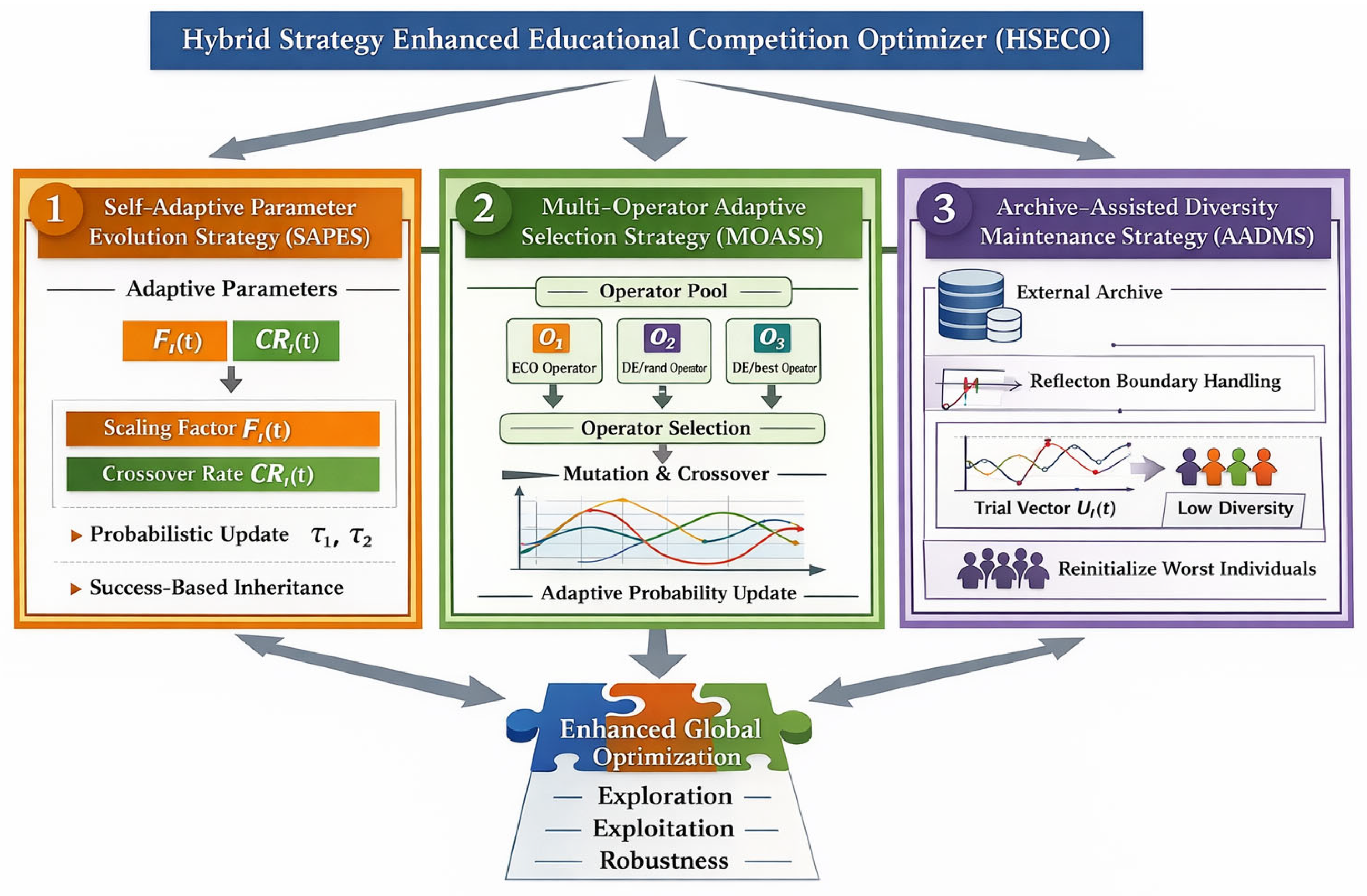
To address these limitations, this paper proposes a Hybrid Strategy Enhanced Educational Competition Optimizer (HSECO) without altering the core educational-stage competition framework of ECO. The proposed method constructs a multi-strategy cooperative enhancement architecture to systematically improve both global exploration and local exploitation capabilities. Specifically, a Self-Adaptive Parameter Evolution Strategy (SAPES) is introduced to allow control parameters to evolve synchronously with candidate solutions, thereby enhancing robustness. A Multi-Operator Adaptive Selection Strategy (MOASS) is designed to integrate the ECO update mechanism with differential evolution operators, dynamically adjusting operator selection probabilities based on online success feedback. In addition, an Archive-Assisted Diversity Maintenance Strategy (AADMS) is incorporated to alleviate premature convergence through historical individual reuse and reflection-based boundary handling. The synergy of these three mechanisms enables HSECO to achieve a more balanced exploration–exploitation trade-off in high-dimensional, multimodal, and heterogeneous composite landscapes.

In recent years, several studies have attempted to improve the performance of the original ECO by introducing enhanced learning strategies, adaptive mechanisms, and hybrid search operators. These ECO variants have demonstrated certain improvements in specific optimization scenarios. However, most of these approaches focus on single-aspect enhancements, such as parameter tuning or local search refinement, and still suffer from limitations in handling high-dimensional, multimodal, and hybrid optimization problems [42,43].

Specifically, existing ECO-based methods often rely on fixed or partially adaptive parameter control schemes, which may lack sufficient flexibility when facing heterogeneous search landscapes. In addition, the update mechanisms in these variants are typically limited to a narrow range of search operators, restricting the diversity of search behaviors. Furthermore, the issue of population diversity loss is not fully addressed, leading to premature convergence in complex optimization environments [44,45].

Compared with these existing improvements, the proposed HSECO introduces a unified hybrid enhancement framework that simultaneously addresses the above limitations. By integrating self-adaptive parameter evolution, multi-operator adaptive selection, and archive-assisted diversity maintenance into a cooperative mechanism, HSECO significantly improves both global exploration capability and local exploitation efficiency. This holistic design enables the algorithm to adapt more effectively to different problem characteristics and enhances its robustness across diverse optimization scenarios.

The main contributions of this work are summarized as follows:

(1)

A hybrid enhancement framework (HSECO) is developed for ECO, integrating adaptive parameter evolution, multi-operator cooperative selection, and archive-assisted diversity maintenance, thereby significantly improving robustness and adaptability.

(2)

Extensive experiments are conducted on the CEC2017, CEC2020, and CEC2022 benchmark suites. Statistical significance is validated using the Wilcoxon rank-sum test and the Friedman average ranking test, comprehensively demonstrating the superiority of HSECO.

(3)

HSECO is applied to a constrained three-dimensional UAV path-planning problem in mountainous terrain. Although the UAV task involves multiple performance responses, namely path length, altitude variation, and turning smoothness, these responses are combined into a single weighted objective function. Thus, the application case is formulated and solved as a single-objective constrained optimization problem, which validates the engineering applicability of HSECO in nonlinear real-world scenarios.

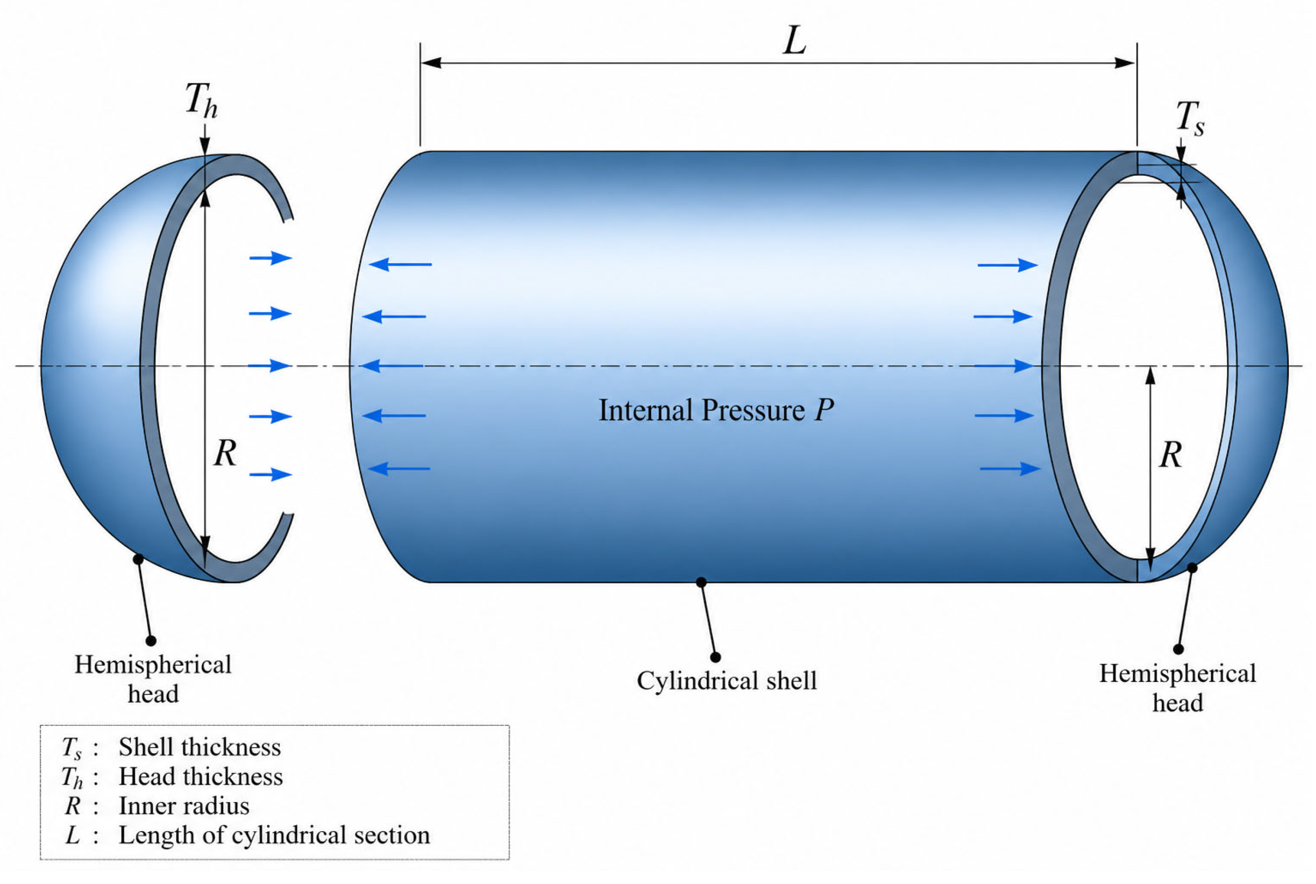
The remainder of this paper is organized as follows. Section 2 introduces the basic principles of ECO and the proposed HSECO framework. Section 3 presents the benchmark experimental design and performance analysis. Section 4 applies HSECO to the three-dimensional UAV path-planning problem. Section 5 evaluates HSECO on the pressure vessel design problem, a classic constrained engineering optimization task. Finally, Section 6 concludes the paper and outlines future research directions.

2. Educational Competition Optimizer and the Proposed Methodology

2.1. Educational Competition Optimizer

The Educational Competition Optimizer (ECO) is a population-based metaheuristic inspired by the progressive learning and competitive mechanisms observed in educational systems [41]. Unlike conventional swarm intelligence algorithms that directly mimic animal or social behaviors, ECO abstracts the hierarchical advancement process of students from primary school to higher educational stages. This staged competition structure provides a natural balance between exploration and exploitation throughout the optimization process.

Assume a minimization problem defined as:

$$\begin{array}{c}minf(X),X\in {\mathbb{R}}^D\end{array}$$

(1)

where $D$ denotes the dimensionality of the decision space. The feasible search region is bounded by lower and upper vectors $lb=[l{b}_1,\dots ,l{b}_D]$ and $ub=[u{b}_1,\dots ,u{b}_D]$. At iteration $t$, the population is represented as [41]:

$$\begin{array}{c}P(t)=\{X_1(t),X_2(t),\dots ,X_N(t)\}\end{array}$$

(2)

where $N$ is the population size and each individual $|X_i(t)=[x_{i,1}(t),\dots ,x_{i,D}(t)].$

After initialization, all individuals are evaluated and sorted in ascending order of fitness. The best and worst solutions at iteration $t$ are denoted as [41]:

$$\begin{array}{c}{X}_{best}(t)=arg \underset{X_i(t)}{min }f(X_i(t)),X_{worst}(t)=arg \underset{X_i(t)}{max }f(X_i(t))\end{array}$$

(3)

ECO divides the search process into three cyclic educational stages, each modeling a different competitive intensity and learning pattern. The stage index is determined according to:

$$\begin{array}{c}S(t)=\mathrm{mod}(t,3)+1\end{array}$$

(4)

Each stage corresponds to a distinct update mechanism, reflecting different learning behaviors.

Stage I: Primary-Level Competition

At this stage, individuals mainly focus on local adjustment and peer imitation. A portion of the top-ranked individuals act as “learning centers,” while the remaining individuals update their positions based on nearby references.

For selected elite individuals, a Lévy-flight-based perturbation is introduced [41]:

$$\begin{array}{c}{X}_i(t+1)=X_i(t)+\omega (t)\cdot \left({\overline{X}}_i(t)-X_i(t)\right)\odot Levy(D)\end{array}$$

(5)

where ${\overline{X}}_i(t)$ denotes the mean component of $X_i(t)$, $\omega (t)$ is a time-dependent step coefficient, and $Levy(D)$ generates heavy-tailed random steps to enhance stochastic exploration.

For non-elite individuals, the update relies on nearest-peer learning [41]:

$$\begin{array}{c}{X}_i(t+1)=X_i(t)+\omega (t)\cdot (X_{near}(t)-X_i(t))\odot \mathcal{N}(\mathrm{0,1})\end{array}$$

(6)

where $X_{near}(t)$ represents the closest superior individual in the ranking sense.

This stage encourages moderate exploration while maintaining structural stability.

Stage II: Intermediate-Level Competition

During the second stage, individuals gradually shift toward more global learning behaviors. The influence of the global best solution increases.

For high-ranking individuals [41]:

$$\begin{array}{c}{X}_i(t+1)=X_i(t)+\left(X_{best}(t)-\overline{X}(t)\right)\cdot exp\left({\displaystyle \frac{t}{T}}-1\right)\odot Levy(D)\end{array}$$

(7)

where $\overline{X}(t)$ is the population mean and $T$ is the maximum iteration number.

For the remaining individuals, competitive pressure is introduced via adaptive directional movement [41]:

$$\begin{array}{c}{X}_i(t+1)=X_i(t)-\omega (t)\cdot X_{near}(t)-P(t)\cdot \left(\kappa (t)\cdot X_{near}(t)-X_i(t)\right)\end{array}$$

(8)

where $P(t)$ and $\kappa (t)$ are dynamic control coefficients regulating competition intensity.

This mechanism increases exploitation strength while retaining stochastic variation.

Stage III: Advanced-Level Competition

In the final stage of each cycle, the search emphasizes strong exploitation around the current best solution [41].

Elite individuals perform symmetric Gaussian perturbations around ${\overline{X}}_i(t)$:

$$\begin{array}{c}{X}_i(t+1)=X_i(t)+\left(X_{best}(t)-{\overline{X}}_i(t)\right)\odot \mathcal{N}(\mathrm{0,1})-\left(X_{worst}(t)-{\overline{X}}_i(t)\right)\odot \mathcal{N}(\mathrm{0,1})\end{array}$$

(9)

Other individuals move directly toward the global best under adaptive scaling:

$$\begin{array}{c}{X}_i(t+1)=X_i(t)-P(t)\cdot \left(X_{best}(t)-X_i(t)\right)\end{array}$$

(10)

This stage significantly accelerates convergence when promising regions have been located.

Boundary Handling and Selection

To ensure feasibility, each dimension is corrected when violating bounds [41]:

$$\begin{array}{c}{X}_{i,d}(t+1)=\left\{\begin{array}{c}\hspace{0.25em}l{b}_d,\hspace{0.25em}\hspace{0.25em}\hspace{0.25em}\hspace{0.25em}\hspace{0.25em}\hspace{0.25em}\hspace{0.25em}\hspace{0.25em}\hspace{0.25em}\hspace{0.25em}\hspace{0.25em} if X_{i,d}(t+1)<l{b}_d,\hfill \\ \hspace{0.25em}u{b}_d,\hspace{0.25em}\hspace{0.25em}\hspace{0.25em}\hspace{0.25em}\hspace{0.25em}\hspace{0.25em}\hspace{0.25em}\hspace{0.25em}\hspace{0.25em}\hspace{0.25em}\hspace{0.25em}if {\hspace{0.25em}X}_{i,d}(t+1)>u{b}_d,\hfill \\ {\hspace{0.25em}X}_{i,d}(t+1),\hspace{0.25em}\hspace{0.25em}\hspace{0.25em}\hspace{0.25em}\mathrm{o}\mathrm{t}\mathrm{h}\mathrm{e}\mathrm{r}\mathrm{w}\mathrm{i}\mathrm{s}\mathrm{e}.\hspace{0.25em}\hspace{0.25em}\hspace{0.25em}\hspace{0.25em}\hfill \end{array}\right.\end{array}$$

(11)

Greedy selection is applied to retain superior solutions:

$$\begin{array}{c}{X}_i(t+1)=\left\{\begin{array}{c}{X}_i(t+1),\hspace{0.25em}\hspace{0.25em}\hspace{0.25em}\hspace{0.25em}if f(X_i(t+1))\le f(X_i(t)),\hfill \\ X_i(t),\hspace{0.25em}\hspace{0.25em}\hspace{0.25em}\hspace{0.25em}\hspace{0.25em}\hspace{0.25em}\hspace{0.25em}\hspace{0.25em}\mathrm{o}\mathrm{t}\mathrm{h}\mathrm{e}\mathrm{r}\mathrm{w}\mathrm{i}\mathrm{s}\mathrm{e}.\hspace{0.25em}\hspace{0.25em}\hspace{0.25em}\hspace{0.25em}\hfill \end{array}\right.\end{array}$$

(12)

The core idea of ECO lies in its cyclical staged competition structure, which alternates between peer learning, global guidance, and intensive refinement. The early stage promotes exploration through Lévy perturbations, the intermediate stage strengthens directional learning from the population and global best, and the advanced stage focuses on local exploitation [41].

Although ECO provides a structured exploration–exploitation transition mechanism, its reliance on fixed-stage scheduling and limited update patterns may restrict adaptability on highly complex, rotated, and hybrid benchmark functions. These limitations motivate the development of the enhanced HSECO framework described in the following sections.

2.2. Proposed Methodology

The original Educational Competition Optimizer (ECO) models the learning–competition process of students across different educational stages. Although ECO is simple and effective on some unimodal or low-dimensional problems, its performance on complex large-scale benchmarks (e.g., CEC2017) is often limited by three practical issues: (i) the search behavior is dominated by a single class of position-updating patterns, which reduces adaptability across heterogeneous landscapes; (ii) the key control factors that regulate step sizes and perturbation intensities are mostly fixed schedules or purely random terms, thus becoming sensitive to problem rotation, modality, and scaling; and (iii) the population diversity can collapse quickly on hybrid and composition functions, leading to premature stagnation and weak late-stage refinement.

To overcome these limitations, this paper proposes the Hybrid Strategy Enhanced Educational Competition Optimizer (HSECO), which constructs a hybrid cooperative search framework on top of ECO. The main idea is to keep ECO’s educational-stage learning philosophy as one search component, while introducing two additional complementary components that are activated and coordinated adaptively. Specifically, HSECO is composed of three mutually reinforcing strategies: Self-Adaptive Parameter Evolution Strategy (SAPES) for robust parameter control, Multi-Operator Adaptive Selection Strategy (MOASS) for landscape-adaptive operator cooperation, and Archive-Assisted Diversity Maintenance Strategy (AADMS) for anti-stagnation and boundary robustness. By integrating these components into a unified iterative scheme, HSECO aims to obtain a more balanced exploration–exploitation behavior and more stable convergence on high-dimensional, rotated, and hybrid objective functions. In summary, the framework of HSECO is illustrated in Figure 1.

2.2.1. Self-Adaptive Parameter Evolution Strategy (SAPES)

A central difficulty when applying ECO to CEC-type problems is that the effective step scale varies significantly across functions and across different search phases. If the algorithm relies on fixed schedules (e.g., a deterministic decay) or purely random coefficients, it may take overly small steps on rugged landscapes or overly large steps near promising basins, which results in unstable convergence and wasted evaluations. HSECO therefore introduces Self-Adaptive Parameter Evolution Strategy (SAPES), which equips each individual with its own evolving control parameters and allows these parameters to be selected by the same “survival-of-the-fittest” principle as candidate solutions.

In SAPES, two control parameters are attached to each individual $X_i\left(t\right)$: a scaling factor $F_i(t)\in [F_l,F_u]$ controlling the magnitude of differential perturbations, and a crossover probability $C{R}_i(t)\in \left[\mathrm{0,1}\right]$ controlling the amount of inherited information from the mutation vector. Instead of manually tuning these parameters, SAPES updates them stochastically with small probabilities ${\tau }_1$ and ${\tau }_2$, respectively. Concretely, when generating a trial solution at iteration $t$, the algorithm first decides whether to refresh $F_i(t)$. If refreshed, $F_i(t)$ is sampled uniformly from $[F_l,F_u]$; otherwise, it inherits $F_i(t-1)$. The same mechanism is applied to $C{R}_i(t)$, where a refreshed value is sampled from [0,1]. This yields the following self-adaptive rule:

$$\begin{array}{c}{\displaystyle \genfrac{}{}{0pt}{}{F_i(t)=\left\{\begin{array}{c}{F}_l+rand\cdot (F_u-F_l),\hspace{0.25em}\hspace{0.25em}\hspace{0.25em}\hspace{0.25em}rand<{\tau }_1,\hfill \\ F_i(t-1),\hspace{0.25em}\hspace{0.25em}\hspace{0.25em}\hspace{0.25em}\hspace{0.25em}\hspace{0.25em}\hspace{0.25em}\hspace{0.25em}\hspace{0.25em}\hspace{0.25em}\hspace{0.25em}\hspace{0.25em}\hspace{0.25em}\hspace{0.25em}\hspace{0.25em} \mathrm{o}\mathrm{t}\mathrm{h}\mathrm{e}\mathrm{r}\mathrm{w}\mathrm{i}\mathrm{s}\mathrm{e},\hspace{0.25em}\hspace{0.25em}\hspace{0.25em}\hspace{0.25em}\hfill \end{array}\right.}{C{R}_i(t)=\left\{\begin{array}{c}rand,\hspace{0.25em}\hspace{0.25em}\hspace{0.25em}\hspace{0.25em}\hspace{0.25em}\hspace{0.25em}\hspace{0.25em}\hspace{0.25em}\hspace{0.25em}\hspace{0.25em}rand<{\tau }_2,\hfill \\ C{R}_i(t-1),\hspace{0.25em}\hspace{0.25em}\hspace{0.25em}\hspace{0.25em}\mathrm{o}\mathrm{t}\mathrm{h}\mathrm{e}\mathrm{r}\mathrm{w}\mathrm{i}\mathrm{s}\mathrm{e}.\hspace{0.25em}\hspace{0.25em}\hspace{0.25em}\hspace{0.25em}\hfill \end{array}\right.}}\end{array}$$

(13)

After the trial solution $U_i(t)$ is evaluated, greedy selection is performed:

$$\begin{array}{c}{X}_i(t+1)=\left\{\begin{array}{c}{U}_i(t),\hspace{0.25em}\hspace{0.25em}\hspace{0.25em}\hspace{0.25em}f(U_i(t))\le f(X_i(t)),\hfill \\ X_i(t),\hspace{0.25em}\hspace{0.25em}\hspace{0.25em}\hspace{0.25em}\mathrm{o}\mathrm{t}\mathrm{h}\mathrm{e}\mathrm{r}\mathrm{w}\mathrm{i}\mathrm{s}\mathrm{e}.\hspace{0.25em}\hspace{0.25em}\hspace{0.25em}\hspace{0.25em}\hfill \end{array}\right.\end{array}$$

(14)

The key design is that the parameters $(F_i(t),C{R}_i(t))$ are kept only when the corresponding trial solution is accepted; otherwise, the previous $(F_i(t-1), C{R}_i(t-1))$ remain. In this manner, parameter configurations that frequently lead to successful improvements are naturally propagated, while ineffective configurations gradually disappear. Compared with fixed or globally scheduled parameters, SAPES provides a low-overhead but robust adaptation mechanism that improves stability across heterogeneous landscapes and reduces the need for manual parameter tuning.

2.2.2. Multi-Operator Adaptive Selection Strategy (MOASS)

Another important limitation of the original ECO is that its update rule is primarily driven by a single behavioral template (stage learning) and thus may not provide sufficient variety of search dynamics. In a real-world problem, different functions demand different behaviors: some require aggressive exploration to escape deceptive basins, while others require strong exploitation to refine in narrow valleys. To address this, HSECO introduces a Multi-Operator Adaptive Selection Strategy (MOASS) that integrates ECO’s stage-learning update with two complementary differential evolution (DE)-style operators, and then adaptively adjusts their usage based on online success feedback.

MOASS maintains an operator pool $|\mathsf{\Omega }=\{{\mathcal{O}}_1,{\mathcal{O}}_2,{\mathcal{O}}_3\}$ and a probability vector $\mathbf{p}(t)=[p_1(t),p_2(t),p_3(t)]$ with ${\displaystyle {\sum }_{k=1}^3}{p}_k(t)=1$. For each individual $X_i(t)$, an operator index $s_i(t)$ is sampled according to $\mathbf{p}(t)$), and the selected operator produces a mutation vector $V_i(t)$. The first operator ${\mathcal{O}}_1$ corresponds to the ECO behavioral update, which preserves the educational-stage learning mechanism and is denoted compactly as:

$$\begin{array}{c}{V}_i(t)=\mathcal{E}\mathcal{C}\mathcal{O}(X_i(t),\mathbf{X}(t),X_{best}(t))\end{array}$$

(15)

This component contributes diversified stochastic learning steps consistent with ECO’s original philosophy.

To enhance exploration on complex multi-modal landscapes, ${\mathcal{O}}_2$ uses a current-to-rand-style differential mutation:

$$\begin{array}{c}{V}_i(t)=X_i(t)+F_i(t)\cdot (X_{r_1}(t)-X_i(t))+F_i(t)\cdot (X_{r_2}(t)-X_{r_3}(t))\end{array}$$

(16)

where $r_1,r_2,r_3$ are mutually distinct indices chosen from the population (and possibly the archive introduced later). This operator encourages directional exploration by combining a pull-away from the current position and a stochastic difference direction.

To strengthen exploitation and accelerate convergence in later search phases, ${\mathcal{O}}_3$ adopts a current-to-best differential form:

$$\begin{array}{c}{V}_i(t)=X_i(t)+F_i(t)\cdot (X_{best}(t)-X_i(t))+F_i(t)\cdot (X_{r_1}(t)-X_{r_2}(t))\end{array}$$

(17)

which directly leverages the current best solution while retaining diversity through a difference vector.

After generating $V_i(t)$, HSECO applies binomial crossover to obtain the trial vector $U_i(t)$:

$$\begin{array}{c}{U}_{i,d}(t)=\left\{\begin{array}{c}{V}_{i,d}(t),\hspace{0.25em}\hspace{0.25em}\hspace{0.25em}\hspace{0.25em}rand\le C{R}_i(t)ord=d_{rand},\\ X_{i,d}(t),\hspace{0.25em}\hspace{0.25em}\hspace{0.25em}\hspace{0.25em}\mathrm{o}\mathrm{t}\mathrm{h}\mathrm{e}\mathrm{r}\mathrm{w}\mathrm{i}\mathrm{s}\mathrm{e},\hspace{0.25em}\hspace{0.25em}\hspace{0.25em}\hspace{0.25em}\hfill \end{array}\right.\end{array}$$

(18)

where $e{d}_{rand}\in \{1,\dots ,D\}$ ensures that at least one dimension is inherited from $V_{i,d}(t)$. The trial vector is then evaluated and accepted by greedy selection (Equation (14)).

The essential feature of MOASS is its online adaptive probability update. HSECO records, within a short sliding window, the number of times each operator is selected (trials) and the number of times it produces an accepted trial solution (successes). Let $T_k(t)$ and $S_k(t)$ denote the trial and success counts of ${\mathcal{O}}_k$. A smoothed success rate is computed as:

$$\begin{array}{c}s{r}_k(t)={\displaystyle \frac{S_k(t)+1}{T_k(t)+3}}\end{array}$$

(19)

The operator probabilities are updated by normalization:

$$\begin{array}{c}{p}_k(t+1)={\displaystyle \frac{s{r}_k(t)}{{\displaystyle {\sum }_{j=1}^3}s{r}_j(t)}},k=\mathrm{1,2},3.\end{array}$$

(20)

To avoid the complete disappearance of any operator (which may be useful at later stages), a minimum probability floor $p_{min}$ is applied and renormalized:

$$\begin{array}{c}{p}_k(t+1)\leftarrow {\displaystyle \frac{p_{min}+(1-3p_{min})p_k(t+1)}{{\displaystyle {\sum }_{j=1}^3}\left[p_{min}+(1-3p_{min})p_j(t+1)\right]}}\end{array}$$

(21)

With MOASS, HSECO can automatically emphasize exploration-oriented operators when the population is trapped and shift toward exploitation-oriented operators when the search enters a promising basin, thereby improving robustness and convergence speed across diverse CEC landscapes.

2.2.3. Archive-Assisted Diversity Maintenance Strategy (AADMS)

Even with adaptive parameters and multiple operators, difficult hybrid/composition functions can still induce rapid diversity loss, causing stagnation and weak late-stage refinement. HSECO therefore introduces the Archive-Assisted Diversity Maintenance Strategy (AADMS), which strengthens diversity through an external archive, improves feasibility handling via reflection boundaries, and triggers controlled diversity injection when the population collapses.

HSECO maintains an external archive $A(t)$ with maximum capacity $A_{max}$. Whenever a trial solution $U_i(t)$ replaces its parent $X_i(t)$, the displaced parent is inserted into the archive:

$$\begin{array}{c}A(t)\leftarrow A(t)\cup \{X_i(t)\},|A(t)|\le A_{max}\end{array}$$

(22)

If the archive is full, a randomly chosen archive element is replaced. During differential mutation in MOASS, a vector participating in the difference term is sampled from the archive with probability $\rho$ (when available), otherwise from the current population:

$$\begin{array}{c}{X}_r(t)\sim \left\{\begin{array}{c}A(t),\hspace{0.25em}\hspace{0.25em}\hspace{0.25em}\hspace{0.25em}rand<\rho \mathrm{and} |A(t)|>0,\\ \mathbf{X}(t),\hspace{0.25em}\hspace{0.25em}\hspace{0.25em}\hspace{0.25em}\mathrm{o}\mathrm{t}\mathrm{h}\mathrm{e}\mathrm{r}\mathrm{w}\mathrm{i}\mathrm{s}\mathrm{e}.\hspace{0.25em}\hspace{0.25em}\hspace{0.25em}\hspace{0.25em}\hfill \end{array}\right.\end{array}$$

(23)

This mechanism introduces “historical diversity” that is often absent in the current population, which is particularly beneficial when many individuals become clustered.

Boundary handling also strongly affects performance on CEC benchmarks. Hard clipping can create boundary attraction and distort the search distribution, especially for large steps. AADMS adopts reflection-based boundary handling to reduce this bias. For each dimension $d$, if $U_{i,d}(t)$ violates the bounds, it is reflected back:

$$\begin{array}{c}{U}_{i,d}(t)=\left\{\begin{array}{c}l{b}_d+(l{b}_d-U_{i,d}(t)),\hspace{0.25em}\hspace{0.25em}\hspace{0.25em}\hspace{0.25em}\hspace{0.25em}if U_{i,d}(t)<l{b}_d,\hfill \\ u{b}_d-(U_{i,d}(t)-u{b}_d),\hspace{0.25em}\hspace{0.25em}\hspace{0.25em} if U_{i,d}(t)>u{b}_d,\\ U_{i,d}(t),\hspace{0.25em}\hspace{0.25em}\hspace{0.25em}\hspace{0.25em}\hspace{0.25em}\hspace{0.25em}\hspace{0.25em}\hspace{0.25em}\hspace{0.25em}\hspace{0.25em}\hspace{0.25em}\hspace{0.25em}\hspace{0.25em}\hspace{0.25em}\hspace{0.25em}\hspace{0.25em}\hspace{0.25em}\hspace{0.25em}\mathrm{o}\mathrm{t}\mathrm{h}\mathrm{e}\mathrm{r}\mathrm{w}\mathrm{i}\mathrm{s}\mathrm{e}.\hspace{0.25em}\hspace{0.25em}\hspace{0.25em}\hspace{0.25em}\hfill \end{array}\right.\end{array}$$

(24)

A final clamp can be applied if repeated reflections still exceed bounds due to extreme steps.

Finally, AADMS monitors the population diversity to prevent irreversible collapse. A normalized diversity indicator is defined as:

$$\begin{array}{c}Div(t)={\displaystyle \frac{1}{D}}{\displaystyle \sum _{d=1}^D}{\displaystyle \frac{std(\{X_{1,d}(t),\dots ,X_{N,d}(t)\})}{u{b}_d-l{b}_d}}\end{array}$$

(25)

If $Div(t)$ falls below a small threshold $\delta =0.02$, a small portion of the worst individuals (e.g., the last $\lfloor \eta N\rfloor \left(\eta =0.1\right)$ individuals after sorting) are re-initialized uniformly within the search range:

$$\begin{array}{c}{X}_{worst}(t)\leftarrow lb+rand\odot (ub-lb)\end{array}$$

(26)

This injection introduces fresh candidates into the population and helps HSECO escape stagnation on complex hybrid/composition landscapes while keeping the overall evaluation budget unchanged.

Based on the above discussion, the pseudocode for HSECO is presented in Algorithm 1.

Algorithm 1. Pseudo-code of the proposed HSECO.

Input: Population size $N$; maximum iterations $T$; dimension $D$; bounds $lb,ub$. Output: Best solution $X_{best}$ and fitness $f\left(X_{best}\right)$. 1: Initialize $\mathbf{x}(0$ within $[lb,ub]$; initialize archive $A\leftarrow \mathrm{\varnothing }.$ 2: Evaluate $f(\mathbf{X}(0))$, sort population, set $X_{best}(0)\leftarrow X_1(0)$. 3: Initialize $\{F_i(0),C{R}_i(0){\}}_{i=1}^N$ and operator probabilities $\mathbf{p}(0)$. 4: while $t=1:T$ do 5:      Compute diversity $Div(t)$ using Equation (25). 6:      for $i=1:N$ 7:            Update $F_i(t),C{R}_i(t)$ via SAPES (Equation (13)). 8:            Select operator $s_i(t)$ according to $\mathbf{p}(t)$. 9:            Generate mutation vector $V_i(t)$ by the chosen operator (Equations (9)–(11)), with archive sampling (Equation (23)). 10:           Generate trial vector $U_i(t)$ by binomial crossover (Equation (18)). 11:           Apply reflection boundary handling (Equation (24)). 12:           Evaluate $f(U_i(t))$ and apply greedy selection (Equation (14)). 13:           If accepted, insert replaced parent into archive (Equation (22)) and record operator success. 14:           Update $X_{best}$ if necessary. 15:     end for 16:     Update operator probabilities $p(t+1)$ using smoothed success rates (Equations (19)–(21)). 17:     If $Div(t)<\delta Div(t)<\delta$, re-initialize a small portion of the worst individuals (Equation (26)). 18: end while 19: Return $X_{best}$ and $f\left(X_{best}\right)$.

2.3. Summary of the Proposed Enhancements

To improve the readability and clarity of the proposed method, this subsection provides a concise summary of the main enhancements introduced in HSECO over the original ECO algorithm.

First, a Self-Adaptive Parameter Evolution Strategy (SAPES) is incorporated to dynamically adjust control parameters at the individual level. Unlike fixed or globally scheduled parameters, SAPES allows successful parameter configurations to be inherited and propagated during the evolutionary process, thereby enhancing robustness and reducing sensitivity to problem characteristics.

Second, a Multi-Operator Adaptive Selection Strategy (MOASS) is introduced to enrich the search dynamics. By integrating multiple search operators, including ECO-based learning and differential evolution mechanisms, HSECO can adaptively select suitable operators according to their historical success rates. This mechanism enables the algorithm to automatically balance exploration and exploitation across different search stages.

Third, an Archive-Assisted Diversity Maintenance Strategy (AADMS) is developed to prevent premature convergence. By maintaining an external archive of historical solutions and introducing diversity-aware reinitialization, this strategy effectively enhances population diversity and improves the ability to escape local optima.

Overall, the combination of SAPES, MOASS, and AADMS forms a hybrid cooperative framework that significantly improves the adaptability, robustness, and optimization performance of the original ECO.

2.4. Complexity Analysis of HSECO

Let $N$ be the population size, $D$ the dimensionality, $T$ the maximum number of iterations, and $f$ the cost of one fitness evaluation. HSECO initializes the population with cost $O(N\cdot D)$ and evaluates the initial fitness with cost $O(N\cdot f)$. During each iteration, each individual generates one trial vector and performs one fitness evaluation, leading to a dominant evaluation cost $O(N\cdot f)$ per iteration. The mutation, crossover, reflection boundary processing, and parameter self-adaptation are vector operations that scale linearly with $D$, resulting in $O(N\cdot D)$ per iteration. Archive maintenance involves constant-time insertions and random replacement, producing at most $O(N)$ overhead per iteration. Updating operator selection probabilities uses only constant-size statistics for three operators and thus costs $O(1)$ per iteration. If sorting is performed each iteration for selecting the worst individuals and tracking the best solution, it adds $O(N\mathrm{l}\mathrm{o}\mathrm{g}N)$.

Therefore, the total time complexity over $T$ iterations can be expressed as $O\left(T\cdot (Nf+ND+N\mathrm{l}\mathrm{o}\mathrm{g}N)\right)$. When fitness evaluation dominates, the complexity simplifies to $O(T\cdot N\cdot f).$ This analysis shows that HSECO preserves the same asymptotic complexity order as standard population-based metaheuristics while adding only modest overhead for adaptive coordination and diversity maintenance, which is justified by its improved robustness on complex benchmark suites.

3. Numerical Experiments

3.1. Competitor Algorithms and Parameters Setting

To evaluate the effectiveness of the proposed HSECO, extensive experiments were conducted on three highly challenging benchmark suites, namely CEC2017, CEC2020, and CEC2022. The performance of HSECO was compared with a variety of representative algorithms.

The comparative algorithms include several enhanced variants of classical optimization methods, such as Enhanced Cooperative Learning and Local Search Integrated Particle Swarm Optimization (ECL-PSO) [46], Enhanced Gray Wolf Optimizer (EGWO) [47], An Improved Sparrow Search Algorithm Based on Quantum Computations and Multi-strategy Enhancement (QMESSA) [48], and Advanced Differential Evolution (ADE) [49]. In addition, recently proposed metaheuristic algorithms were also considered, including Jaya algorithm (JAYA) [50], Kangaroo Escape Optimization (KEO) [51], Rüppell’s Fox Optimizer (RFO) [52], Birds of Prey-Based Optimization (BPBO) [53], as well as the standard Educational Competition Optimizer (ECO) [41]. To ensure a fair comparison, all competing algorithms were implemented using the parameter settings recommended in their original publications. The configuration details of all benchmark algorithms are summarized in

Table 1. Compare algorithm parameter settings.

Algorithms	Name of the Parameter	Value of the Parameter
ECL-PSO	$w,c_1,c_2,c_3,q_m{Prob}_{ls}$	[0.5,0.9], [2,0], [0,2], [0,2], 0.4, 0.1
EGWO	$a,std\text{\_}dev$	$2 to 0, exp(-100t/T)$
QMESSA	$ST,PD, SD,ED$	0.8, 0.2, 0.2, 0.2
ADE	${pop}_{min}, { pop}_{init},{ p}_{CR}$	4, 28, 0.2
JAYA	$r_1,r_2$	$N(0, 1), N(0, 1)$
KEO	$\mathrm{E}\mathrm{n}\mathrm{e}\mathrm{r}\mathrm{g}\mathrm{y} \mathrm{t}\mathrm{h}\mathrm{r}\mathrm{e}\mathrm{s}\mathrm{h}\mathrm{o}\mathrm{l}\mathrm{d}, \beta$	0.5, 0.5
RFO	$a_0,a_1,c_0,c_1$, $e_0,e_1$ $\beta$	2, 3, 2, 2, 1, 3, 0.000001
BPBO	$P_i$	0.7
ECO	$H,G_1,G_2$	$0.5, 0.2, 0.1$

.

To ensure methodological consistency and reduce the impact of random fluctuations, all algorithms were evaluated under identical experimental settings. The population size was uniformly set to 30 individuals, and the maximum number of iterations was limited to 500. Each algorithm was independently executed 30 times to obtain statistically reliable results. The performance was assessed using statistical indicators, including the average value (Mean) and the standard deviation (Std), with the best results highlighted in bold for clarity.

All simulations were carried out on a computer running the Windows 11 operating system, equipped with an Intel^® Core™ i5-13400 (13th Generation) processor operating at a base frequency of 2.5 GHz and 16 GB of RAM. The algorithms were implemented and executed using MATLAB R2024b.

3.2. Qualitative Analysis

3.2.1. Ablation Study

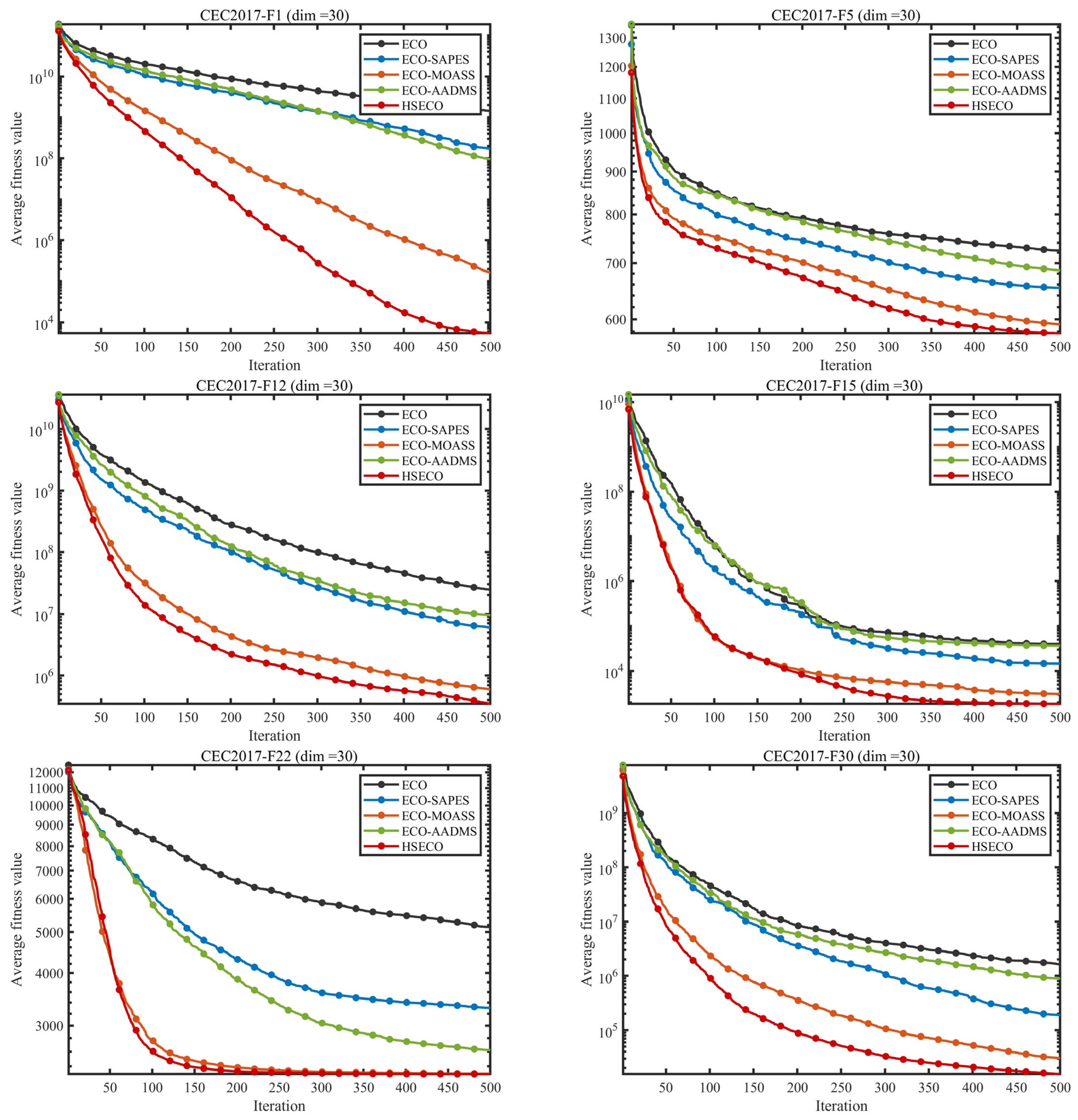
To evaluate the individual contribution of each proposed strategy, an ablation study was conducted on the CEC2017 benchmark suite with a dimensionality of 30. Specifically, five algorithm variants were designed and compared, including the baseline ECO, ECO enhanced with the Self-Adaptive Parameter Evolution Strategy (SAPES), ECO integrated with the Multi-Operator Adaptive Selection Strategy (MOASS), ECO combined with the Archive-Assisted Diversity Maintenance Strategy (AADMS), and the complete HSECO model incorporating all proposed strategies. To ensure a fair comparison, all variants were evaluated under identical experimental settings, including the same population size, maximum number of iterations, and number of independent runs. The comparative results are presented in Figure 2.

As illustrated in Figure 2, on the unimodal function F1, the original ECO exhibits a relatively fast convergence rate in the early iterations; however, it stagnates after approximately 100 iterations, leading to limited final accuracy. After incorporating the SAPES, the late-stage convergence capability is significantly improved, and the convergence curve continues to decline until the end of the iterations, indicating that the self-adaptive parameter mechanism effectively maintains search vitality. With the further introduction of the MOASS, the convergence speed is further accelerated, and the curve becomes steeper, demonstrating that the multi-operator adaptive selection mechanism enhances the global search efficiency. The complete HSECO model achieves the best final convergence accuracy on F1, with its convergence curve consistently remaining below those of all other variants.

On the multimodal function F4 and the hybrid function F11, the original ECO shows a pronounced premature convergence behavior, with the convergence curves flattening at an early stage. Both ECO + SAPES and ECO + MOASS can alleviate this issue to some extent; however, their individual improvements are limited. Notably, ECO + AADMS demonstrates a strong ability to escape local optima on F4 and F11, where the convergence curves exhibit multiple stepwise declines, confirming the effectiveness of the Archive-Assisted Diversity Maintenance Strategy on complex multimodal and hybrid functions. By integrating the advantages of all three strategies, the complete HSECO model not only achieves the fastest convergence but also maintains a continuous downward trend throughout the entire iteration process, ultimately attaining significantly superior convergence accuracy compared to all single-strategy variants.

On the composition functions F22 and F25, both the original ECO and the single-strategy variants suffer from different degrees of stagnation in local optima, accompanied by noticeable fluctuations in the convergence curves. In contrast, HSECO exhibits the most stable and consistent descending behavior, with a smooth convergence curve and the best final convergence value. On F30, the performance differences among the variants become particularly evident: HSECO continues to achieve further improvements after approximately 250 iterations, whereas the other variants have already stagnated.

Overall, from all subplots in Figure 2, it can be observed that each of the three strategies contributes to the performance enhancement of ECO. Specifically, SAPES primarily improves the parameter self-adaptation capability, MOASS enhances the dynamic balance between exploration and exploitation, and AADMS plays a crucial role in maintaining population diversity. Their synergistic integration enables HSECO to achieve optimal or near-optimal convergence performance across all test functions, thereby establishing a solid algorithmic foundation for subsequent comprehensive experiments.

3.2.2. Parameter Sensitivity Analysis

In the Archive-Assisted Diversity Maintenance Strategy (AADMS), the parameter η controls the proportion of the worst individuals that are re-initialized when the population diversity falls below a predefined threshold (δ = 0.02). Specifically, $\lfloor \eta N\rfloor$ individuals are randomly regenerated within the search space, as defined in Equation (26). This mechanism plays a critical role in restoring population diversity and preventing premature convergence.

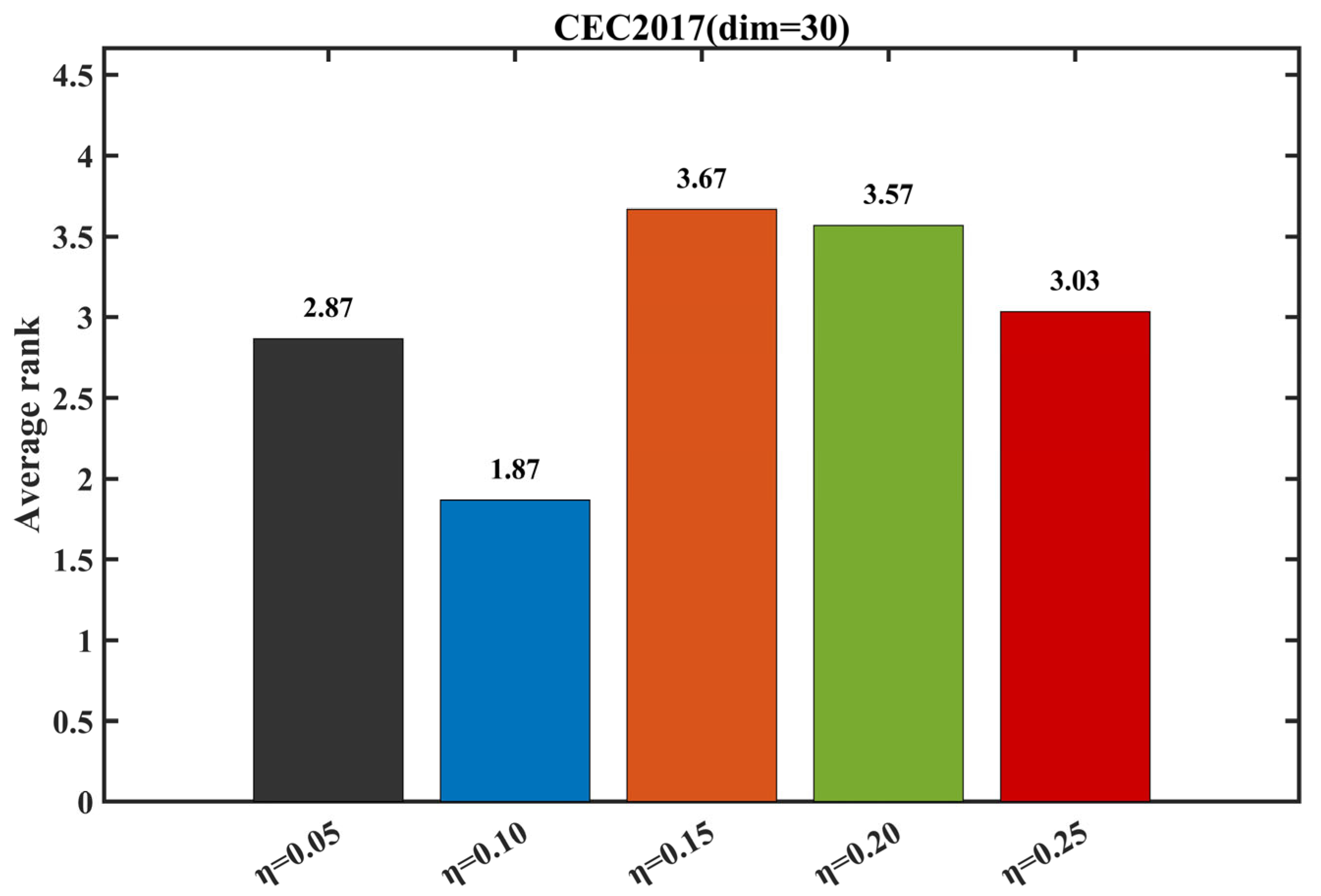
To investigate the influence of η on the performance of HSECO, a parameter sensitivity analysis was conducted by testing five representative values: $\eta$ = 0.05, 0.10, 0.15, 0.20, and 0.25. The experiments were carried out on selected functions from the CEC2017 benchmark suite under identical experimental settings. The ranking results under different parameter values are shown in Figure 3.

As observed from Figure 3, the average ranking of HSECO varies significantly with different values of $\eta$. When $\eta$ = 0.10, HSECO achieves the best average ranking (1.87), indicating that this setting provides an optimal balance between diversity maintenance and convergence stability. When η = 0.05, the average ranking is 2.87. Although the performance remains competitive, it is inferior to that of $\eta$ = 0.10. This is because a smaller reinitialization ratio is insufficient to effectively introduce new individuals when population diversity is severely reduced, which may still lead to premature convergence on certain functions.

When $\eta$ = 0.15, 0.20, and 0.25, the average rankings are 3.67, 3.57, and 3.03, respectively, all of which are worse than the optimal result obtained at $\eta$ = 0.10. In particular, for $\eta$ = 0.15 and 0.20, the average rankings exceed 3.5, suggesting that an excessively high reinitialization ratio leads to frequent replacement of individuals, thereby disrupting the useful information accumulated in the population and weakening the local exploitation capability of the algorithm. Although the average ranking improves to 3.03 at $\eta$ = 0.25, it still does not outperform the configuration with $\eta$ = 0.10.

Based on the above analysis, $\eta$ = 0.10 is identified as the optimal parameter setting for HSECO, and this value is adopted in all subsequent experiments.

3.2.3. Exploration and Exploitation Analysis

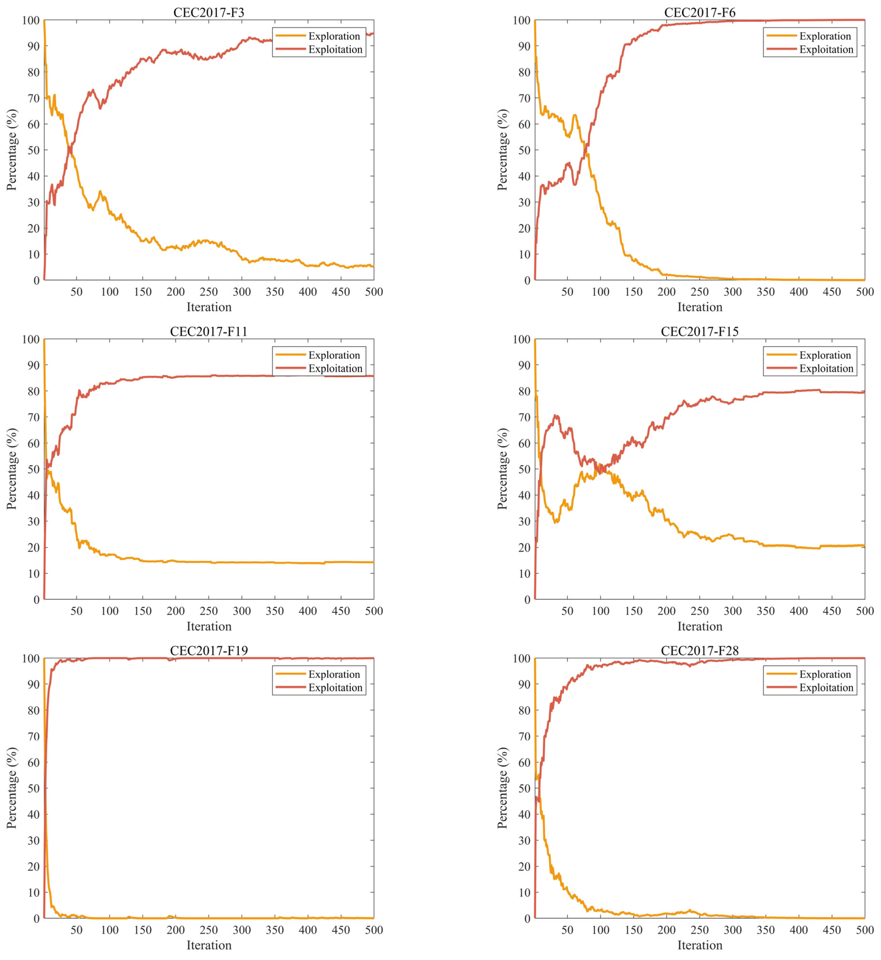
To further reveal the search behavior characteristics of HSECO during the optimization process, this subsection provides a quantitative analysis of the dynamic balance between exploration and exploitation on the CEC2017 benchmark suite. Exploration refers to the algorithm’s ability to investigate new regions of the search space, whereas exploitation denotes its capability to perform refined searches in promising areas. A proper balance between these two behaviors is crucial for achieving superior performance in metaheuristic algorithms. As shown in Figure 4, the variation curves of exploration and exploitation ratios over iterations are presented for six representative benchmark functions.

It can be observed from Figure 4 that, during the early stage of optimization (the first 50 iterations), the exploration ratio is significantly higher than the exploitation ratio across all functions. For instance, on F1 and F4, the initial exploration ratios reach approximately 0.85 and 0.80, respectively. This indicates that HSECO primarily emphasizes global exploration in the early phase, enabling broad coverage of the search space and effectively reducing the risk of being trapped in poor local optima. As the iteration progresses, the exploration ratio gradually decreases, while the exploitation ratio correspondingly increases. This trend is particularly evident on F11 and F22, where the crossover point between exploration and exploitation occurs around the 150th to 200th iterations, after which exploitation becomes the dominant behavior.

It is worth noting that the rates of change and final convergence proportions of exploration and exploitation differ across functions. On the relatively simple function F1, the exploration ratio declines rapidly and stabilizes at approximately 0.35 after around 150 iterations, indicating that the algorithm can quickly transition from global exploration to local refinement. In contrast, for more complex functions such as F25 and F30, the exploration ratio remains relatively high throughout the optimization process, staying above 0.40 even after 400 iterations. This demonstrates that HSECO can adaptively maintain a strong exploration capability according to problem complexity, thereby effectively addressing the challenges posed by multimodal landscapes with numerous local optima.

Overall, HSECO exhibits a smooth transition from exploration-dominated to exploitation-dominated behavior across all six benchmark functions, without premature decline in exploration or delayed activation of exploitation. This progressive behavioral shift validates the effectiveness of the proposed multi-operator adaptive selection mechanism and the Archive-Assisted Diversity Maintenance Strategy. Their synergistic interaction enables HSECO to maintain a well-balanced exploration–exploitation trade-off at different stages of the optimization process, resulting in excellent convergence performance across various types of benchmark functions.

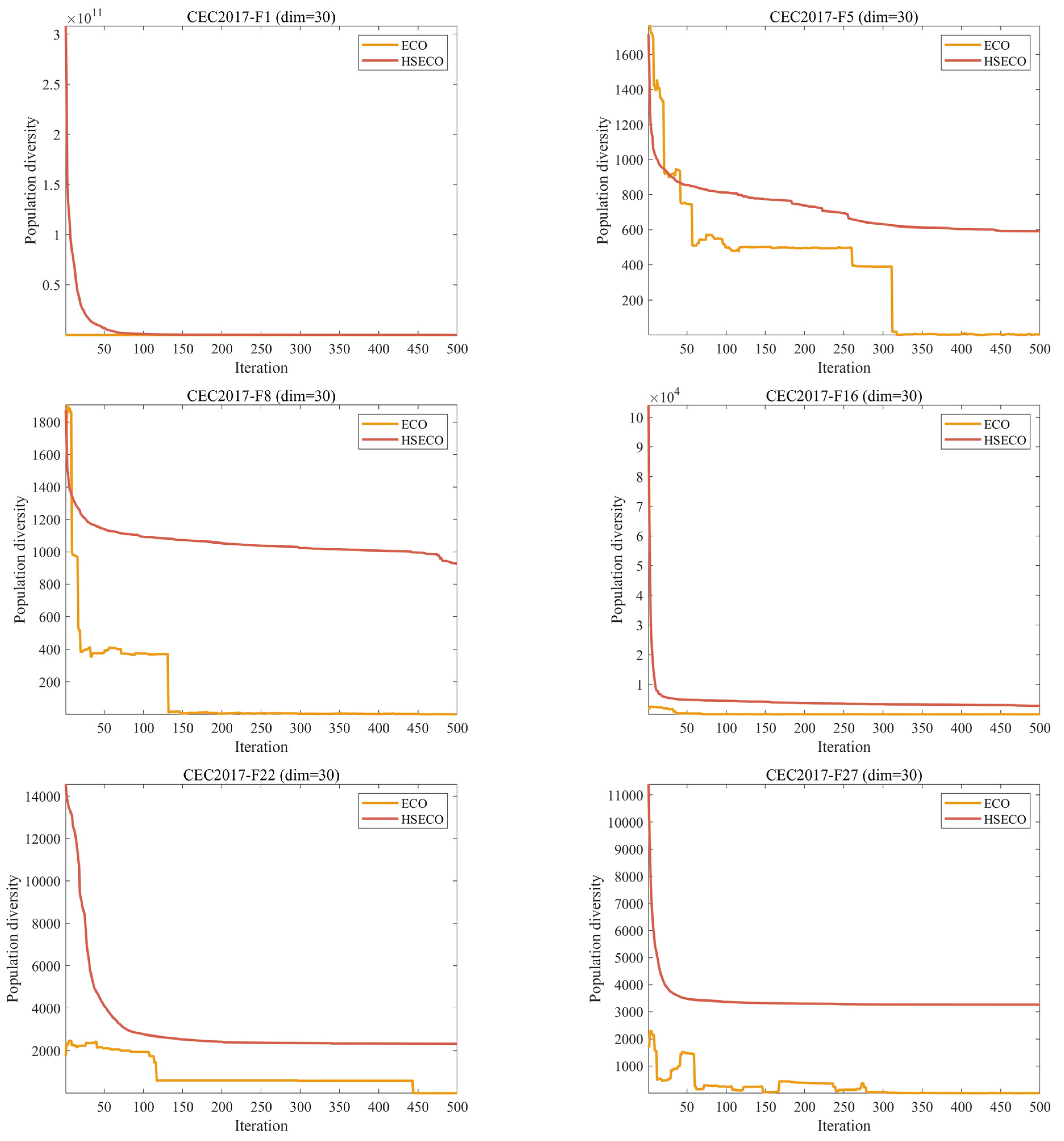
3.2.4. Population Diversity Analysis

To further investigate the global exploration capability and dynamic search characteristics of the proposed HSECO algorithm, a comparative analysis of population diversity between HSECO and the original ECO is conducted on the 30-dimensional CEC2017 benchmark functions. Population diversity intuitively reflects the dispersion degree of individuals in the search space during the iterative process and serves as a crucial indicator for evaluating the global exploration ability of an algorithm as well as its effectiveness in preventing premature convergence.

As illustrated in Figure 5, the population diversity curves of different algorithms show that, in the early stage of iteration, both ECO and HSECO maintain relatively high diversity levels, indicating that individuals are widely distributed across the search space. This provides a solid foundation for extensive global exploration in the initial phase. However, as the number of iterations increases, the population diversity of the original ECO declines rapidly. After the mid-iteration stage, the diversity drops to a low level and remains in this range throughout the subsequent iterations. This behavior suggests that the population of ECO quickly converges to a local region, with reduced differences among individuals, making it prone to premature convergence, especially on complex multimodal, hybrid, and composition functions.

In contrast, HSECO consistently maintains significantly higher population diversity than the original ECO throughout the entire optimization process. Moreover, the decline in diversity is more gradual and stable, without any abrupt collapse. Even in the later stages of iteration, HSECO is able to preserve a relatively higher level of population dispersion. This can be attributed to the synergistic effect of the Archive-Assisted Diversity Maintenance Strategy and the adaptive operator selection mechanism, which effectively slow down the loss of diversity. On complex test cases such as multimodal, hybrid, and composition functions, the diversity advantage of HSECO over ECO becomes even more pronounced, continuously providing sufficient search vitality and reducing the probability of being trapped in local optima.

Overall, by integrating the proposed diversity maintenance and adaptive search strategies, HSECO achieves a stable preservation of population diversity while balancing global exploration and local exploitation. This effectively overcomes the shortcomings of the original ECO, such as rapid diversity loss and susceptibility to premature convergence in complex optimization problems, thereby providing critical support for efficient global optimization in high-dimensional and complex search spaces.

3.3. Experimental Results and Analysis of CEC Test Suites

3.3.1. Experimental Results and Analysis of CEC2017 Test Suite

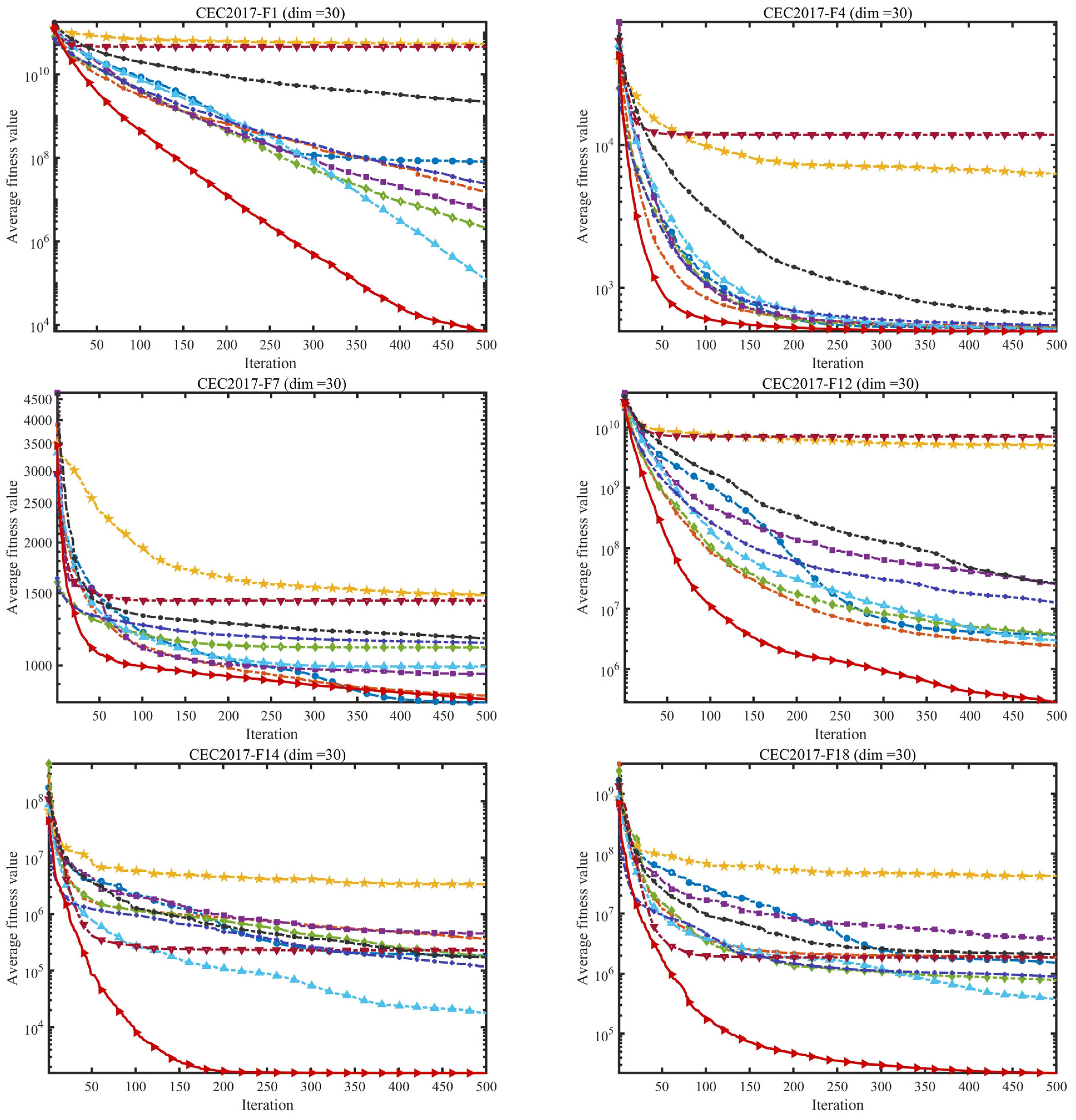
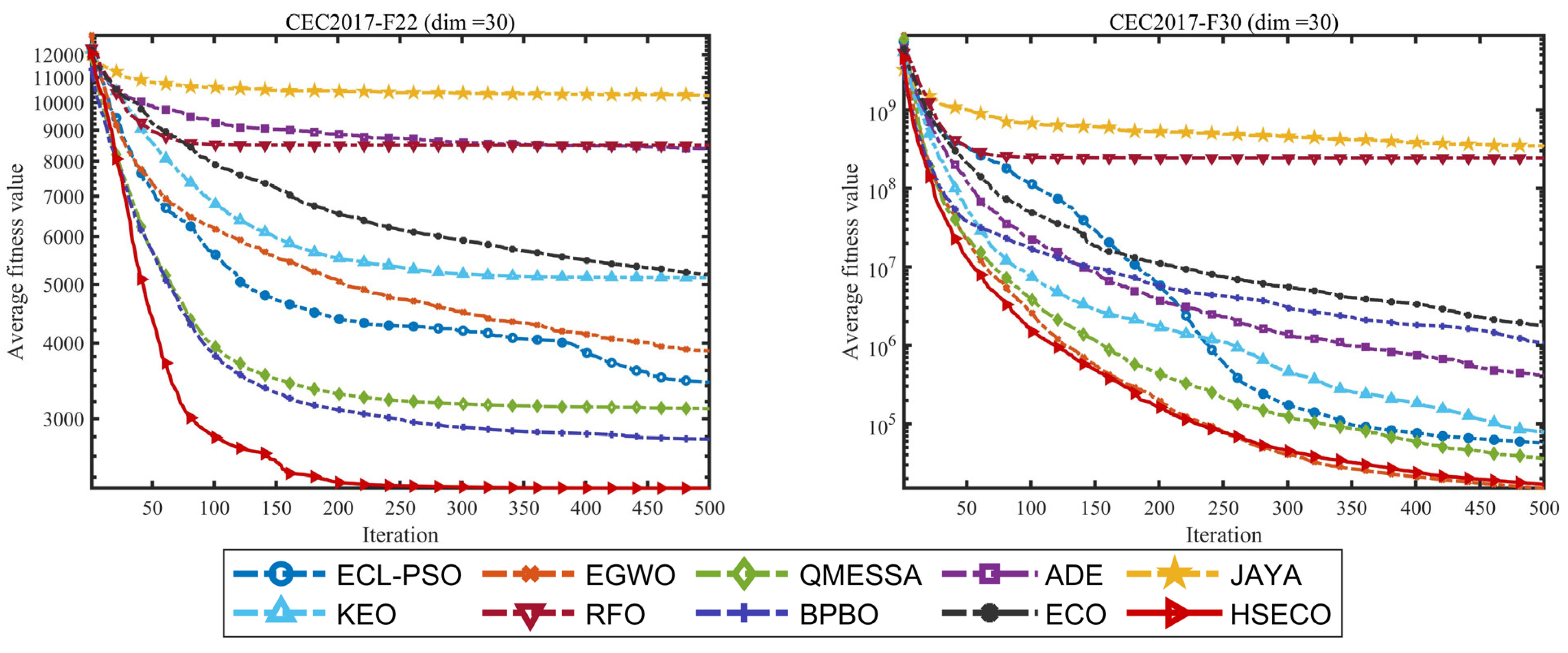
To verify the performance superiority of the proposed HSECO algorithm in high-dimensional and complex optimization scenarios, comparative experiments were conducted on the CEC2017 30-dimensional benchmark test suite. This benchmark set includes unimodal, multimodal, hybrid, and composition functions, which comprehensively evaluate an algorithm’s global exploration capability, local exploitation ability, and convergence stability. In this study, HSECO was compared with nine representative State-of-the-Art metaheuristic algorithms (ECL-PSO, EGWO, QMESSA, ADE, JAYA, KEO, RFO, BPBO, and ECO) under identical experimental settings. The performance was evaluated from multiple perspectives, including the average fitness value (Ave), standard deviation (Std), and convergence behavior, to objectively assess the optimization effectiveness and robustness of HSECO. The experimental results are presented in Figure 6 and

Table 2. Experimental results of CEC2017 (dim = 30).

Function	Metric	ECL-PSO	EGWO	QMESSA	ADE	JAYA	KEO	RFO	BPBO	ECO	HSECO
F1	Ave	8.1517E+07	1.5208E+07	2.0953E+06	5.3025E+06	5.3580E+10	1.2144E+05	4.5820E+10	2.4148E+07	2.1952E+09	7.0417E+03
	Std	3.0775E+08	1.4718E+07	1.5373E+06	2.7364E+06	9.1428E+09	9.1909E+04	1.4206E+10	1.1202E+07	1.6575E+09	5.4593E+03
F2	Ave	1.0569E+31	1.6308E+20	6.7320E+20	3.0774E+31	3.2065E+43	4.6482E+19	4.1979E+46	1.6066E+24	5.3169E+30	5.3720E+16
	Std	5.2873E+31	7.5599E+20	3.1546E+21	8.1169E+31	1.0532E+44	1.5118E+20	2.2936E+47	8.4638E+24	2.0282E+31	2.3560E+17
F3	Ave	8.0228E+04	1.1927E+05	5.5920E+04	1.5134E+05	3.0519E+05	4.3407E+04	9.2982E+04	5.3562E+04	5.8440E+04	1.2500E+04
	Std	2.1780E+04	5.0889E+04	6.8262E+03	3.0927E+04	5.5138E+04	1.9637E+04	2.6975E+04	7.6131E+03	1.4533E+04	4.4808E+03
F4	Ave	5.2550E+02	5.2908E+02	5.2345E+02	5.1330E+02	6.2959E+03	5.1797E+02	1.1808E+04	5.4623E+02	6.5975E+02	4.9592E+02
	Std	2.5442E+01	2.5011E+01	3.4911E+01	1.5619E+01	2.1041E+03	3.5285E+01	4.2756E+03	2.5177E+01	7.9605E+01	3.2129E+01
F5	Ave	5.6374E+02	5.8184E+02	7.1697E+02	6.9916E+02	9.2680E+02	6.3559E+02	8.5923E+02	7.2411E+02	7.2469E+02	5.8163E+02
	Std	1.7520E+01	2.7716E+01	3.9117E+01	1.5081E+01	3.9738E+01	3.6851E+01	4.3920E+01	4.1067E+01	3.8637E+01	2.3851E+01
F6	Ave	6.0438E+02	6.0367E+02	6.5038E+02	6.0093E+02	6.8254E+02	6.2830E+02	6.7412E+02	6.5975E+02	6.5076E+02	6.0102E+02
	Std	2.3348E+00	2.3641E+00	6.8809E+00	2.6181E−01	1.2288E+01	8.5488E+00	1.3075E+01	8.5590E+00	9.9968E+00	1.0600E+00
F7	Ave	8.1150E+02	8.4235E+02	1.1066E+03	9.5272E+02	1.4862E+03	9.9339E+02	1.4396E+03	1.1344E+03	1.1649E+03	8.2542E+02
	Std	1.9679E+01	4.0638E+01	7.2746E+01	1.6745E+01	1.1782E+02	8.6460E+01	1.2713E+02	1.2020E+02	8.6818E+01	2.1754E+01
F8	Ave	8.6054E+02	8.7875E+02	9.7553E+02	9.9128E+02	1.1807E+03	9.2677E+02	1.0986E+03	9.6938E+02	9.6475E+02	8.7169E+02
	Std	1.8084E+01	1.9541E+01	3.1828E+01	1.6688E+01	3.3012E+01	2.1211E+01	3.7097E+01	2.5494E+01	3.4093E+01	1.9608E+01
F9	Ave	1.1288E+03	2.1733E+03	4.9722E+03	2.0838E+03	1.5655E+04	2.9596E+03	1.0686E+04	5.6222E+03	5.7424E+03	1.1810E+03
	Std	3.0430E+02	1.4270E+03	4.3485E+02	5.6393E+02	3.3987E+03	8.0403E+02	2.8616E+03	1.4394E+03	8.5853E+02	4.9448E+02
F10	Ave	5.5731E+03	4.8601E+03	5.1572E+03	7.4915E+03	9.0186E+03	5.0407E+03	8.4236E+03	6.2286E+03	6.0694E+03	5.1764E+03
	Std	1.8364E+03	1.5310E+03	6.0504E+02	3.4628E+02	2.4028E+02	7.8435E+02	6.4274E+02	1.2943E+03	8.8700E+02	8.9561E+02
F11	Ave	1.3271E+03	1.5013E+03	1.2647E+03	1.9377E+03	2.6928E+04	1.2983E+03	6.4526E+03	1.3277E+03	1.5893E+03	1.2314E+03
	Std	6.9933E+01	4.5841E+02	5.4870E+01	4.9332E+02	9.1334E+03	6.3913E+01	2.7438E+03	4.6177E+01	3.0096E+02	5.3714E+01
F12	Ave	3.7511E+06	2.4566E+06	3.8409E+06	2.5276E+07	5.1084E+09	2.9691E+06	7.0403E+09	1.2635E+07	2.6568E+07	2.8313E+05
	Std	4.7338E+06	2.4499E+06	3.0246E+06	1.7952E+07	1.7932E+09	2.4433E+06	4.7822E+09	1.0909E+07	1.9380E+07	2.2837E+05
F13	Ave	2.4557E+04	1.1429E+04	7.8862E+03	2.5454E+06	4.4036E+08	3.7630E+04	3.1682E+09	1.4787E+05	1.8946E+05	1.0493E+04
	Std	2.4265E+04	1.1649E+04	6.3320E+03	3.5953E+06	3.6806E+08	2.7100E+04	3.4358E+09	1.6886E+05	1.3858E+05	1.0301E+04
F14	Ave	1.8361E+05	3.6564E+05	1.7120E+05	4.5316E+05	3.3934E+06	1.7758E+04	2.2920E+05	1.1832E+05	1.7252E+05	1.5492E+03
	Std	1.8988E+05	2.7333E+05	1.0981E+05	2.8163E+05	2.2192E+06	1.6044E+04	5.0782E+05	1.1875E+05	3.3499E+05	3.9975E+01
F15	Ave	8.5651E+03	5.9288E+03	2.8445E+03	8.9129E+05	3.2904E+08	1.4852E+04	1.9609E+07	1.5078E+04	3.6468E+04	1.7833E+03
	Std	1.0789E+04	6.0868E+03	1.2984E+03	6.8774E+05	3.3006E+08	1.1768E+04	9.0990E+07	7.1516E+03	3.3146E+04	1.1995E+02
F16	Ave	2.4875E+03	2.6184E+03	3.0134E+03	2.9970E+03	5.3629E+03	2.7567E+03	4.2578E+03	3.0380E+03	3.1102E+03	2.3189E+03
	Std	3.2229E+02	3.6548E+02	3.6775E+02	1.6934E+02	5.7776E+02	3.6160E+02	9.0696E+02	3.3878E+02	4.6362E+02	2.5480E+02
F17	Ave	1.9897E+03	2.1161E+03	2.3595E+03	2.2355E+03	3.4909E+03	2.2311E+03	2.6892E+03	2.4219E+03	2.3537E+03	1.8904E+03
	Std	1.5375E+02	2.0054E+02	1.9650E+02	9.7997E+01	2.7609E+02	1.8359E+02	4.5176E+02	2.6699E+02	1.8009E+02	8.7353E+01
F18	Ave	1.5139E+06	1.8856E+06	7.8143E+05	3.8361E+06	4.2661E+07	3.7948E+05	1.8665E+06	8.9430E+05	2.1323E+06	2.2049E+04
	Std	1.8948E+06	1.8808E+06	8.0234E+05	2.4477E+06	2.5273E+07	4.2169E+05	3.7060E+06	1.2323E+06	3.0838E+06	1.3342E+04
F19	Ave	1.1492E+04	6.9517E+03	4.7618E+03	7.6475E+05	3.2600E+08	1.2927E+04	1.2839E+07	6.1984E+04	6.5941E+04	2.0082E+03
	Std	1.2936E+04	6.3694E+03	2.2708E+03	7.0281E+05	1.8091E+08	1.2264E+04	1.9613E+07	1.1062E+05	1.5602E+05	7.1784E+01
F20	Ave	2.3804E+03	2.5744E+03	2.7473E+03	2.5303E+03	3.1245E+03	2.6625E+03	2.7903E+03	2.6381E+03	2.7320E+03	2.2192E+03
	Std	1.6169E+02	1.9586E+02	2.6421E+02	1.1173E+02	1.1859E+02	2.6058E+02	2.5225E+02	1.7670E+02	2.0181E+02	1.0201E+02
F21	Ave	2.3695E+03	2.3749E+03	2.4737E+03	2.4994E+03	2.6902E+03	2.4135E+03	2.6359E+03	2.4665E+03	2.5146E+03	2.3684E+03
	Std	1.9174E+01	2.1280E+01	8.5796E+01	1.1233E+01	3.9561E+01	2.6465E+01	4.5378E+01	3.6359E+01	5.6796E+01	2.1862E+01
F22	Ave	3.4442E+03	3.8805E+03	3.1150E+03	8.3932E+03	1.0271E+04	5.1303E+03	8.4971E+03	2.7753E+03	5.1848E+03	2.3019E+03
	Std	2.1511E+03	1.8965E+03	1.6679E+03	1.4746E+03	3.9726E+02	2.0907E+03	1.5227E+03	1.5584E+03	2.5770E+03	2.5329E+00
F23	Ave	2.7410E+03	2.7224E+03	2.8808E+03	2.8399E+03	3.4322E+03	2.8049E+03	3.5267E+03	2.8947E+03	2.9308E+03	2.7322E+03
	Std	2.2261E+01	2.1852E+01	7.2845E+01	1.5602E+01	1.1141E+02	5.1903E+01	1.7372E+02	6.3804E+01	9.5929E+01	2.7875E+01
F24	Ave	2.9082E+03	2.9044E+03	3.0418E+03	3.0398E+03	3.5664E+03	2.9680E+03	3.8336E+03	3.0151E+03	3.1141E+03	2.8984E+03
	Std	3.4132E+01	4.7404E+01	7.8197E+01	1.6524E+01	1.0037E+02	4.0551E+01	2.3844E+02	5.6359E+01	8.4802E+01	2.3874E+01
F25	Ave	2.9280E+03	2.9217E+03	2.9179E+03	2.9036E+03	3.7943E+03	2.9257E+03	4.9316E+03	2.9839E+03	3.0086E+03	2.8984E+03
	Std	2.5922E+01	3.4345E+01	2.4779E+01	7.2734E+00	3.9546E+02	2.8040E+01	7.8577E+02	2.7489E+01	3.7055E+01	1.4977E+01
F26	Ave	4.2265E+03	4.3853E+03	5.5696E+03	5.5872E+03	1.2407E+04	5.6081E+03	9.9203E+03	6.6476E+03	6.3209E+03	4.4656E+03
	Std	4.6481E+02	5.9986E+02	1.8308E+03	1.3784E+02	1.0451E+03	8.0233E+02	1.3770E+03	1.5492E+03	8.2288E+02	7.2788E+02
F27	Ave	3.2305E+03	3.2280E+03	3.3076E+03	3.2273E+03	3.6424E+03	3.2706E+03	4.2257E+03	3.3527E+03	3.2767E+03	3.2390E+03
	Std	1.7773E+01	1.4303E+01	4.0920E+01	5.6479E+00	1.1497E+02	3.0710E+01	3.9093E+02	9.2779E+01	3.0988E+01	1.9629E+01
F28	Ave	3.3029E+03	3.3019E+03	3.2746E+03	3.3048E+03	6.2883E+03	3.2869E+03	6.4734E+03	3.3220E+03	3.5283E+03	3.2445E+03
	Std	4.1486E+01	4.1746E+01	2.1422E+01	1.9238E+01	1.1175E+03	3.1299E+01	1.2564E+03	3.0627E+01	1.6998E+02	2.4811E+01
F29	Ave	3.7567E+03	3.7656E+03	4.2257E+03	4.2623E+03	6.1644E+03	4.2191E+03	5.5798E+03	4.4828E+03	4.5616E+03	3.6979E+03
	Std	1.8218E+02	2.0738E+02	2.6354E+02	1.6748E+02	5.6736E+02	4.0568E+02	8.0833E+02	2.9129E+02	3.1688E+02	1.4979E+02
F30	Ave	5.6909E+04	1.5117E+04	3.6060E+04	4.1392E+05	3.3960E+08	7.8017E+04	2.4329E+08	1.0782E+06	1.7786E+06	1.7002E+04
	Std	4.5108E+04	8.2670E+03	2.7652E+04	4.3519E+05	1.1776E+08	9.3278E+04	2.5834E+08	1.3076E+06	1.9703E+06	9.1201E+03

.

From the statistical results in Table 2, it can be observed that HSECO achieves the best mean values on the majority of the 30 test functions. Specifically, on F1, HSECO attains a mean value of 7.0417E+03, which is significantly better than ECO (2.1952E+09) and other comparison algorithms, with an improvement exceeding five orders of magnitude. On F2, HSECO achieves a mean value of 5.3720E+16, substantially outperforming ECO (5.3169E+30) and JAYA (3.2065E+43), demonstrating a strong capability in locating extreme optima. Moreover, on multiple functions such as F3, F4, F12, F14, F18, and F19, HSECO consistently obtains the best mean results, accompanied by relatively small standard deviations, indicating excellent stability.

It is worth noting that HSECO does not achieve the best performance on all functions. For instance, on F5, ECL-PSO achieves the best mean value of 5.6374E+02, while HSECO ranks second with 5.8163E+02. On F6, ADE slightly outperforms HSECO, with mean values of 6.0093E+02 and 6.0102E+02, respectively. Similarly, ECL-PSO attains the best results on F7 and F8. These observations indicate that certain comparison algorithms exhibit advantages on specific functions; however, HSECO still maintains competitive performance on these cases, with differences remaining within an acceptable range.

From the perspective of standard deviation, HSECO achieves the smallest Std values on functions such as F1, F2, F3, F12, F14, F18, and F19. For example, on F14, the Std of HSECO is only 3.9975E+01, which is significantly lower than those of the other algorithms. This demonstrates that HSECO not only provides high optimization accuracy but also exhibits strong robustness with low variability across multiple independent runs.

The convergence curves in Figure 6 further illustrate the dynamic optimization behaviors of the algorithms. On F1, the convergence curve of HSECO remains consistently lower than those of the other algorithms from the initial stage and continues to decrease throughout the entire iteration process without noticeable stagnation. In contrast, algorithms such as ECO, JAYA, and RFO enter a plateau after approximately 100 iterations. On F2, HSECO exhibits a very rapid convergence rate, reaching a low fitness level within the first 50 iterations and continuing to improve steadily thereafter. Similar superiority is observed on F4 and F11, where HSECO achieves both the fastest convergence speed and the highest final accuracy. On the complex composition functions F22 and F30, the convergence curve of HSECO shows a stepwise descending pattern, indicating its ability to escape local optima multiple times and continuously refine the solution quality, whereas most comparison algorithms stagnate in the later stages.

In summary, based on the analyses of Table 2 and Figure 6, HSECO achieves the highest number of best mean results on the CEC2017 30-dimensional benchmark suite, with both convergence speed and final accuracy significantly outperforming the original ECO and nine other comparison algorithms. The statistical results confirm that the effective integration of self-adaptive parameter evolution, multi-operator cooperative selection, and Archive-Assisted Diversity Maintenance Strategy substantially enhances the overall optimization capability of HSECO in high-dimensional multimodal and complex composition landscapes.

3.3.2. Experimental Results and Analysis of the CEC2020 Test Suite

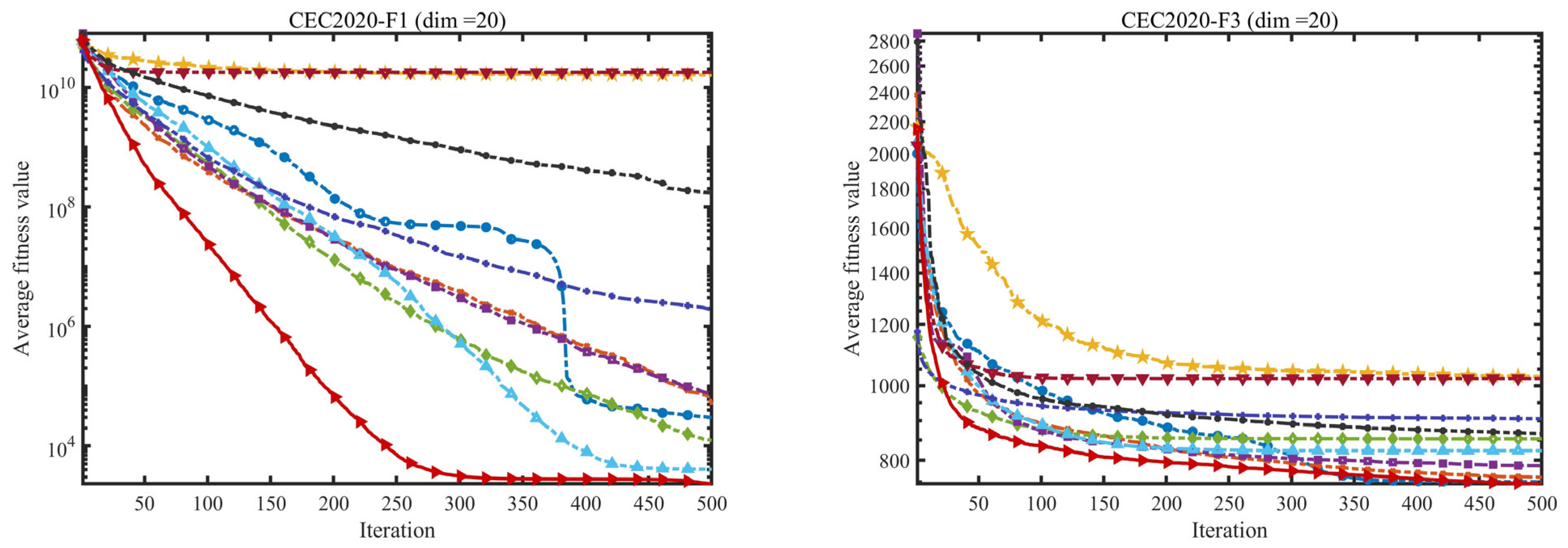
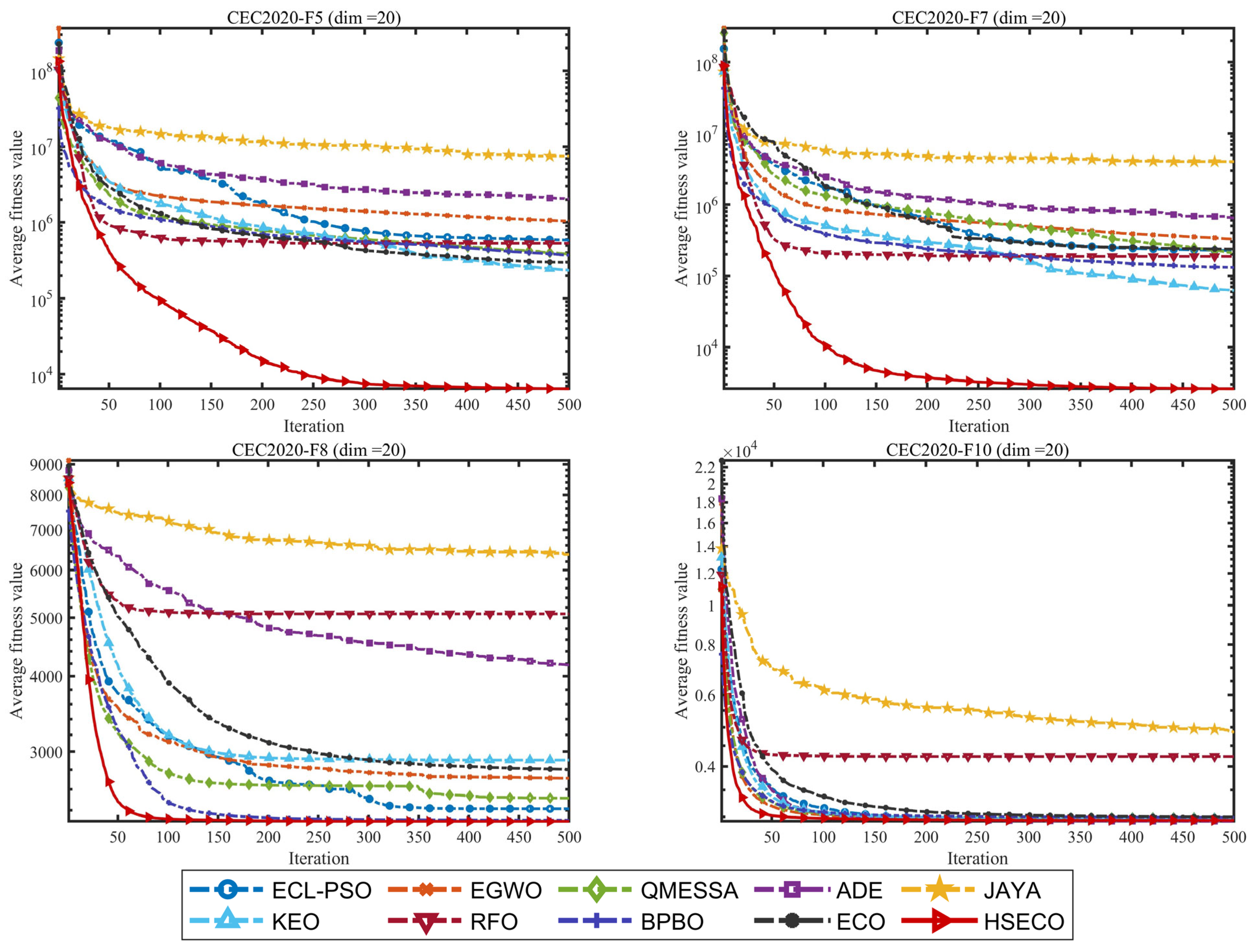
To further validate the generalization capability and adaptability of HSECO in medium-dimensional complex optimization scenarios, additional comparative experiments were conducted on the CEC2020 benchmark suite with a dimensionality of 20. The CEC2020 test set emphasizes heterogeneous landscapes and composite optimization characteristics, which makes it particularly suitable for evaluating an algorithm’s global exploration capability and precise exploitation performance across problems of varying dimensionality and complexity. Under identical experimental settings, HSECO was compared with nine benchmark algorithms. The performance was analyzed using the average fitness value, standard deviation, and convergence curves to comprehensively assess optimization accuracy, stability, and convergence speed on the CEC2020 test suite. The experimental results are presented in Figure 7 and

Table 3. Experimental results of CEC2020 (dim = 20).

Function	Metric	ECL-PSO	EGWO	QMESSA	ADE	JAYA	KEO	RFO	BPBO	ECO	HSECO
F1	Ave	2.9749E+04	4.8772E+04	1.2332E+04	7.4921E+04	1.6086E+10	4.0706E+03	1.7851E+10	1.8753E+06	1.7281E+08	2.3223E+03
	Std	6.2700E+04	7.9212E+04	1.7453E+04	4.9649E+04	2.8849E+09	3.2896E+03	7.2914E+09	1.5351E+06	3.5092E+08	2.4328E+03
F2	Ave	2.4557E+03	2.6543E+03	2.7425E+03	2.9492E+03	5.1839E+03	2.8545E+03	5.0097E+03	3.2672E+03	3.1586E+03	2.1766E+03
	Std	4.5437E+02	1.4220E+03	4.8917E+02	1.9241E+02	2.6173E+02	4.7103E+02	4.6986E+02	5.1533E+02	5.0325E+02	3.8144E+02
F3	Ave	7.5025E+02	7.6042E+02	8.5295E+02	7.8729E+02	1.0275E+03	8.2338E+02	1.0212E+03	9.0557E+02	8.6672E+02	7.4564E+02
	Std	9.2745E+00	1.9832E+01	2.6544E+01	9.6467E+00	3.9971E+01	3.1075E+01	9.1874E+01	4.3154E+01	3.7153E+01	9.1165E+00
F4	Ave	1.9035E+03	1.9044E+03	1.9179E+03	1.9087E+03	4.7555E+04	1.9096E+03	2.1723E+05	1.9195E+03	1.9224E+03	1.9039E+03
	Std	1.4315E+00	2.9407E+00	9.7904E+00	1.1297E+00	2.5405E+04	3.1155E+00	3.0305E+05	5.7637E+00	1.0858E+01	1.6299E+00
F5	Ave	5.8482E+05	1.0434E+06	3.8031E+05	2.0512E+06	7.5016E+06	2.3476E+05	5.2990E+05	3.7082E+05	2.9690E+05	6.4393E+03
	Std	4.2625E+05	8.7810E+05	1.7652E+05	1.1025E+06	3.7323E+06	2.2292E+05	9.2317E+05	1.8560E+05	2.3968E+05	5.4757E+03
F6	Ave	4.7284E+03	2.9146E+03	2.4667E+03	1.1296E+04	2.5977E+03	2.4061E+03	2.1127E+03	3.4983E+03	4.9002E+03	1.8171E+03
	Std	5.5328E−01	1.2656E+01	3.1887E+00	4.0582E−01	2.9705E+00	4.0497E+00	1.7451E+01	3.2222E+00	5.7414E+00	3.4606E−01
F7	Ave	2.2591E+05	3.2752E+05	2.1155E+05	6.5050E+05	4.0183E+06	6.2369E+04	1.8746E+05	1.3172E+05	2.3839E+05	2.6050E+03
	Std	1.9766E+05	3.7222E+05	1.5044E+05	3.9818E+05	2.9495E+06	5.9484E+04	3.8125E+05	9.5061E+04	3.1467E+05	2.8921E+02
F8	Ave	2.4133E+03	2.7137E+03	2.5132E+03	4.1791E+03	6.3755E+03	2.9073E+03	5.0768E+03	2.3106E+03	2.8049E+03	2.3006E+03
	Std	3.8721E+02	9.4592E+02	8.0673E+02	1.4142E+03	1.3001E+03	1.1368E+03	1.1916E+03	2.3356E+00	1.2257E+03	6.4533E−01
F9	Ave	2.8439E+03	2.8466E+03	2.8651E+03	2.9045E+03	3.1662E+03	2.8688E+03	3.2509E+03	2.8913E+03	2.9665E+03	2.8383E+03
	Std	1.2959E+01	2.0606E+01	1.4736E+02	1.1081E+01	5.9857E+01	2.8387E+01	1.2049E+02	3.1164E+01	8.0058E+01	1.2174E+01
F10	Ave	2.9460E+03	2.9627E+03	2.9810E+03	2.9261E+03	4.8586E+03	2.9654E+03	4.2338E+03	2.9925E+03	2.9998E+03	2.9421E+03
	Std	3.5007E+01	3.3659E+01	3.0321E+01	2.3535E+01	1.0992E+03	3.6396E+01	7.3836E+02	2.0863E+01	4.4859E+01	3.4530E+01

.

From the statistical results in Table 3, it can be observed that HSECO achieves the best mean values on the majority of the ten test functions. On F1, HSECO attains a mean value of 2.3223E+03, which is significantly superior to ECO (1.7281E+08) and other comparison algorithms, with an improvement exceeding five orders of magnitude, demonstrating a strong search capability. On F5, HSECO achieves a mean value of 6.4393E+03, substantially outperforming KEO (2.3476E+05) and ECO (2.9690E+05), showing a remarkable advantage. On F6, HSECO obtains the best mean value of 1.8171E+03, significantly better than RFO (2.1127E+03) and ECO (4.9002E+03). On F7, HSECO achieves a mean value of 2.6050E+03, far surpassing all comparison algorithms, where KEO ranks second with 6.2369E+04, indicating an advantage of more than one order of magnitude. In addition, HSECO also achieves the best mean results on F8 and F9.

It is worth noting that HSECO does not rank first on all functions. On F2, ECL-PSO achieves the best mean value of 2.4557E+03, while HSECO ranks second with 2.1766E+03. On F3, ADE slightly outperforms HSECO with a mean value of 6.0007E+02, although the difference between the two is negligible. On F4, ECL-PSO achieves the best mean value of 1.9035E+03, marginally better than HSECO (1.9039E+03), with an extremely small gap. On F10, ADE achieves the best mean value of 2.9261E+03, outperforming HSECO (2.9421E+03). These results indicate that although HSECO does not achieve the top rank on a few functions, it consistently maintains optimal or near-optimal performance, with only marginal differences from the leading algorithms.

From the perspective of standard deviation, HSECO achieves the smallest Std values on multiple functions, including F1, F5, F6, F7, and F8. Notably, on F8, the standard deviation of HSECO is only 6.4533E−01, which is significantly lower than that of other algorithms, indicating excellent stability and consistency. On F6, the Std of HSECO is 3.4606E−01, also markedly better than those of the comparison algorithms. These results demonstrate that HSECO not only achieves high optimization accuracy but also exhibits strong robustness with minimal variation across independent runs.

The convergence curves in Figure 7 further illustrate the dynamic optimization behaviors of the algorithms. On F1, the convergence curve of HSECO remains significantly lower than those of all other algorithms from the initial stage and continues to decrease throughout the entire iteration process without any stagnation. In contrast, algorithms such as ECO, JAYA, and RFO enter a plateau after approximately 50 iterations. On F5, HSECO converges extremely rapidly, reaching a very low fitness level within the first 100 iterations, while other algorithms tend to be trapped in local optima or converge slowly. On F6, the convergence curve of HSECO exhibits a rapid decline followed by stable convergence, ultimately achieving significantly better accuracy than the comparison algorithms. On F7 and F8, HSECO again demonstrates the fastest convergence speed and the highest final accuracy. On F10, although ADE achieves slightly better final accuracy than HSECO, the convergence curve of HSECO is smoother, and the difference between the two remains minimal.

In summary, based on the analyses of Table 3 and Figure 7, HSECO achieves the best mean results on seven out of 10 functions (F1, F5, F6, F7, F8, and F9) in the CEC2020 20-dimensional benchmark suite, while ranking second on the remaining three functions with only marginal differences from the best results. Compared with the original ECO, HSECO achieves significant improvements on all ten functions, particularly on F1, F5, and F7, where the improvements span several orders of magnitude. These results fully demonstrate the superiority, stability, and strong generalization capability of HSECO in medium-dimensional heterogeneous optimization scenarios.

3.3.3. Experimental Results and Analysis of CEC2022 Test Suite

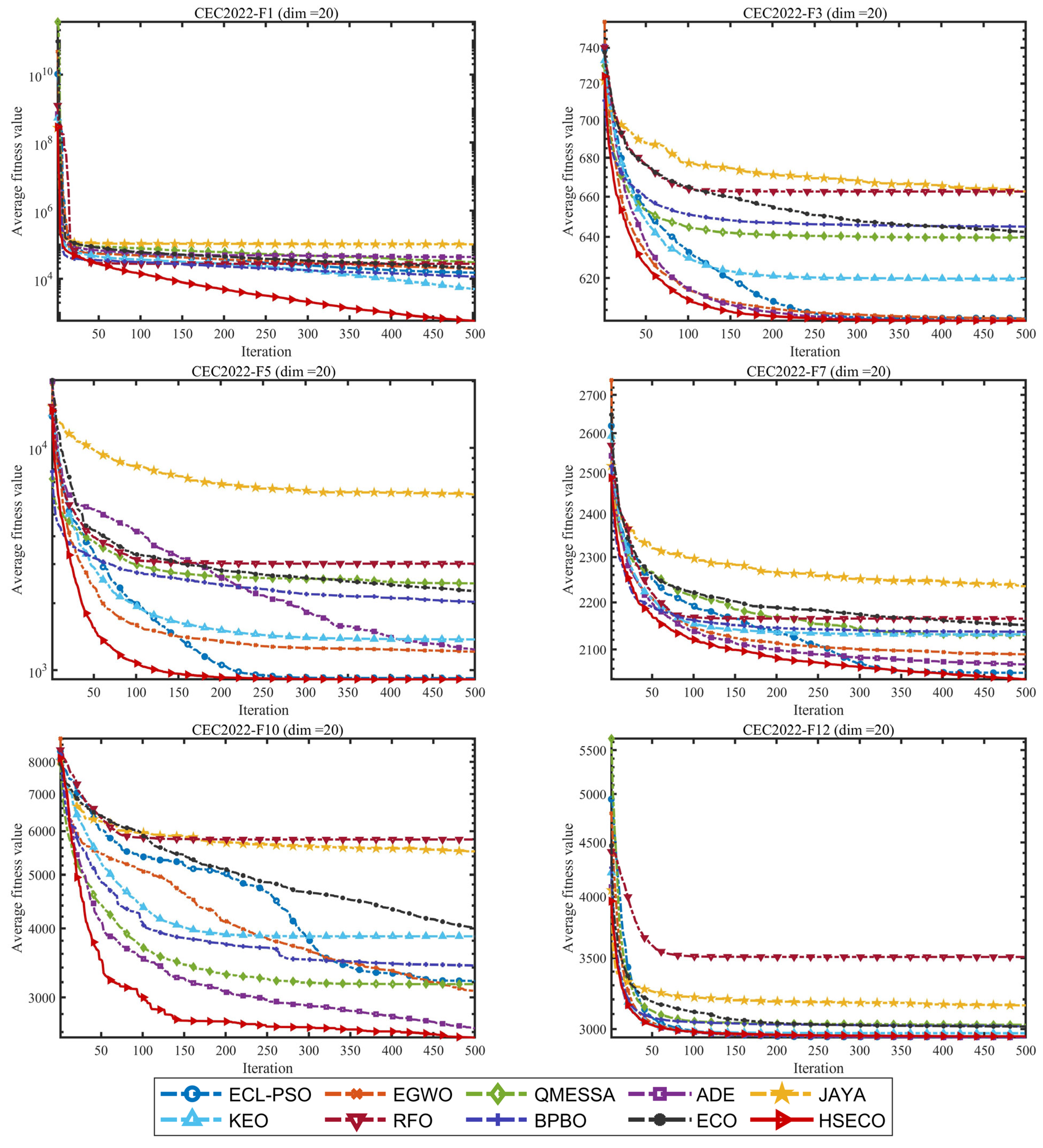
To further evaluate the adaptability and robustness of HSECO in heterogeneous and composite optimization environments, additional comparative experiments were conducted on the CEC2022 benchmark suite (20-dimensional). The CEC2022 test set integrates more nonlinear and highly coupled characteristics, posing greater challenges to an algorithm’s landscape adaptability and diversity preservation capability. Under unified experimental settings, HSECO was compared with nine mainstream metaheuristic algorithms. The performance was assessed using the average fitness value, standard deviation, and convergence curves to comprehensively analyze optimization accuracy, stability, and convergence efficiency on this benchmark suite. The experimental results are presented in Figure 8 and

Table 4. Experimental results of CEC2022 (dim = 20).

Function	Metric	ECL-PSO	EGWO	QMESSA	ADE	JAYA	KEO	RFO	BPBO	ECO	HSECO
F1	Ave	1.5119E+04	2.0210E+04	3.0231E+04	4.3681E+04	1.0219E+05	5.0080E+03	2.7422E+04	1.1519E+04	2.1709E+04	5.8862E+02
	Std	8.2258E+03	8.1174E+03	1.2732E+04	1.0772E+04	2.7884E+04	3.9007E+03	8.6314E+03	4.7353E+03	1.0398E+04	2.6489E+02
F2	Ave	4.5547E+02	4.5683E+02	4.6674E+02	4.4920E+02	1.5443E+03	4.6607E+02	1.4172E+03	4.7021E+02	5.1728E+02	4.5309E+02
	Std	1.1600E+01	1.2133E+01	2.8391E+01	3.4561E−01	4.3292E+02	1.8564E+01	4.9237E+02	1.9978E+01	4.5554E+01	1.8621E+01
F3	Ave	6.0127E+02	6.0107E+02	6.3963E+02	6.0007E+02	6.6276E+02	6.1970E+02	6.6267E+02	6.4500E+02	6.4233E+02	6.0007E+02
	Std	1.0068E+00	1.1630E+00	1.0931E+01	2.7577E−02	1.0019E+01	1.0634E+01	1.5662E+01	1.1325E+01	1.0978E+01	9.9534E−02
F4	Ave	8.2964E+02	8.4287E+02	8.9064E+02	9.1848E+02	9.9062E+02	8.6158E+02	9.4068E+02	8.7867E+02	8.8248E+02	8.3610E+02
	Std	1.1884E+01	1.5800E+01	1.0100E+01	1.1204E+01	1.7910E+01	1.8916E+01	2.2719E+01	1.2212E+01	2.0609E+01	1.0381E+01
F5	Ave	9.2065E+02	1.2109E+03	2.4582E+03	1.2388E+03	6.1636E+03	1.3735E+03	3.0100E+03	2.0307E+03	2.2692E+03	9.0963E+02
	Std	2.5754E+01	4.2931E+02	1.8760E+02	1.9484E+02	1.8754E+03	3.7439E+02	7.3982E+02	5.9624E+02	4.0530E+02	2.3271E+01
F6	Ave	4.1873E+03	4.7388E+03	4.5871E+03	4.0703E+06	4.3238E+08	6.8572E+03	2.0971E+08	7.6243E+03	1.6088E+04	2.9569E+03
	Std	3.7652E+03	3.6427E+03	2.6146E+03	2.5908E+06	2.9892E+08	4.8275E+03	5.0745E+08	1.9513E+04	1.7638E+04	2.4639E+03
F7	Ave	2.0518E+03	2.0898E+03	2.1299E+03	2.0693E+03	2.2354E+03	2.1317E+03	2.1647E+03	2.1370E+03	2.1512E+03	2.0390E+03
	Std	1.9039E+01	5.0005E+01	4.4900E+01	1.4059E+01	4.3067E+01	5.8151E+01	5.6480E+01	3.0696E+01	6.2101E+01	7.7190E+00
F8	Ave	2.2445E+03	2.2562E+03	2.2547E+03	2.2320E+03	2.2724E+03	2.2636E+03	2.3348E+03	2.2868E+03	2.2671E+03	2.2300E+03
	Std	4.0751E+01	5.1543E+01	5.4224E+01	2.5121E+00	2.0987E+01	5.9206E+01	1.1020E+02	5.6525E+01	5.9555E+01	2.1522E+01
F9	Ave	2.4850E+03	2.4834E+03	2.4811E+03	2.4808E+03	2.8361E+03	2.4809E+03	2.8066E+03	2.4858E+03	2.4983E+03	2.4808E+03
	Std	1.2180E+01	2.0776E+00	4.0312E−01	1.0502E−02	7.7286E+01	1.6539E-01	1.0878E+02	5.0238E+00	1.2181E+01	8.4036E−05
F10	Ave	3.2133E+03	3.0820E+03	3.1740E+03	2.6414E+03	5.5147E+03	3.8728E+03	5.7918E+03	3.4258E+03	4.0154E+03	2.5418E+03
	Std	6.4211E+02	9.8743E+02	4.1921E+02	1.7630E+02	1.6632E+03	7.4126E+02	1.5494E+03	1.1445E+03	7.7283E+02	1.6554E+02
F11	Ave	3.0354E+03	2.9446E+03	2.9474E+03	2.9161E+03	7.8210E+03	2.9600E+03	6.7201E+03	2.9748E+03	3.2450E+03	2.9159E+03
	Std	2.4785E+02	1.3580E+02	9.4853E+01	8.3502E+01	1.2817E+03	1.4973E+02	1.1189E+03	1.4669E+02	2.8797E+02	9.9485E+01
F12	Ave	2.9493E+03	2.9541E+03	3.0286E+03	2.9463E+03	3.1594E+03	2.9735E+03	3.5091E+03	3.0181E+03	3.0166E+03	2.9542E+03
	Std	1.0299E+01	1.1322E+01	1.1498E+02	3.5027E+00	8.5627E+01	2.0816E+01	1.8655E+02	4.0672E+01	7.1881E+01	1.2889E+01

.

From the statistical results in Table 4, it can be observed that HSECO achieves the best mean values on the majority of the twelve test functions. On F1, HSECO attains a mean value of 5.8862E+02, which is significantly better than KEO (5.0080E+03) and ECO (2.1709E+04), representing an improvement of nearly two orders of magnitude. On F5, HSECO achieves the best mean value of 9.0963E+02, clearly outperforming ECL-PSO (9.2065E+02) and ECO (2.2692E+03). On F6, HSECO obtains the best mean value of 2.9569E+03, significantly superior to KEO (6.8572E+03) and ECO (1.6088E+04). On F7, HSECO achieves a mean value of 2.0390E+03, outperforming ECL-PSO (2.0518E+03) and ECO (2.1512E+03). HSECO also achieves the best mean results on F8 and F9; notably, on F9, the standard deviation of HSECO is as low as 8.4036E−05, indicating extremely high convergence accuracy and stability. Furthermore, on F10, F11, and F12, HSECO also attains the best or near-best mean values.

It is worth noting that HSECO does not rank first on all functions. On F2, ADE achieves the best mean value of 4.4920E+02, while HSECO ranks second with 4.5309E+02, with only a negligible difference. On F3, both ADE and HSECO obtain the same mean value of 6.0007E+02, indicating equivalent accuracy, although the standard deviation of HSECO (9.9534E−02) is slightly larger than that of ADE (2.7577E−02). On F4, ECL-PSO achieves the best mean value of 8.2964E+02, marginally outperforming HSECO (8.3610E+02). On F12, ADE slightly outperforms HSECO with a mean value of 2.9463E+03 compared to 2.9542E+03. These results indicate that although HSECO does not achieve the top rank on a few functions, it consistently maintains optimal or near-optimal performance, with only marginal differences from the leading algorithms.

From the perspective of standard deviation, HSECO achieves the smallest Std values on multiple functions, including F1, F5, F6, F7, and F9. Particularly on F9, the Std of HSECO is only 8.4036E−05, making it the only algorithm to reach such a level of precision, which demonstrates its exceptional convergence consistency and robustness. On F7, the Std of HSECO is 7.7190E+00, significantly better than ECO (6.2101E+01) and other comparison algorithms. These results further confirm that HSECO not only achieves high optimization accuracy but also exhibits very low variability across multiple independent runs.

The convergence curves in Figure 8 further illustrate the dynamic optimization behaviors of the algorithms. On F1, the convergence curve of HSECO remains significantly lower than those of all other algorithms from the initial stage and maintains a continuous and stable downward trend throughout the entire iteration process, without any sign of stagnation. In contrast, algorithms such as ECO, JAYA, and RFO enter a plateau after approximately 50 iterations. On F5, HSECO converges noticeably faster than the other algorithms, reaching a low fitness level within the first 100 iterations, whereas the other algorithms generally converge slowly or become trapped in local optima. On F6, the convergence curve of HSECO shows a rapid decline followed by continuous improvement, ultimately achieving significantly better accuracy than the comparison algorithms. On F7 and F9, HSECO again demonstrates the fastest convergence speed and the highest final accuracy, with the convergence curve on F9 remaining at the lowest level throughout almost all iterations. On F10 and F11, although algorithms such as ADE and ECL-PSO perform comparably to HSECO in certain stages, HSECO continues to achieve further improvements in the later stages, demonstrating stronger sustained search capability.

In summary, based on the analyses of Table 4 and Figure 8, HSECO achieves the best mean results on eight out of 12 functions (F1, F5, F6, F7, F8, F9, F10, and F11) in the CEC2022 20-dimensional benchmark suite, while ranking second or third on the remaining four functions with only marginal differences from the leading algorithms. Compared with the original ECO, HSECO achieves significant improvements on all twelve functions, particularly on F1, F5, and F6, where the improvements range from several times to tens of times. These results convincingly demonstrate that even in strongly coupled and highly nonlinear heterogeneous composite optimization landscapes, HSECO maintains statistically reliable performance gains, thereby validating the synergistic effectiveness of the three proposed hybrid strategies.

3.4. Statistical Analysis

3.4.1. Wilcoxon Rank-Sum Test Analysis

To statistically validate the significance and reliability of the performance improvements achieved by HSECO, the Wilcoxon rank-sum test was employed at a significance level of $p=0.05$. The test was conducted between HSECO and nine competing algorithms across the CEC2017, CEC2020, and CEC2022 benchmark suites. By counting the number of functions on which HSECO significantly outperforms (+), performs equivalently (=), or underperforms (−) relative to each competitor, the statistical superiority of the proposed algorithm under different dimensionalities and varying optimization complexities is quantitatively assessed.

The Wilcoxon rank-sum test results summarized in

Table 5. Results for various algorithms on the CEC test set.

HSECO VS.	ECL-PSO	EGWO	QMESSA	ADE	JAYA	KEO	RFO	BPBO	ECO
CEC2017 (+/=/−)	(23/0/7)	(21/0/9)	(27/0/3)	(26/0/4)	(30/0/0)	(28/0/2)	(30/0/0)	(30/0/0)	(30/0/0)
CEC2020 (+/=/−)	(6/0/4)	(7/0/3)	(10/0/0)	(10/0/0)	(9/0/1)	(10/0/0)	(10/0/0)	(10/0/0)	(10/0/0)
CEC2022 (+/=/−)	(9/0/3)	(7/0/5)	(10/0/2)	(10/0/2)	(11/0/1)	(11/0/1)	(12/0/0)	(12/0/0)	(12/0/0)

clearly illustrate the distribution of performance superiority of HSECO over the nine comparison algorithms across the three CEC benchmark suites. From a statistical perspective, these results further confirm the overall superiority and strong adaptability of HSECO. Notably, no statistically equivalent cases (=) are observed in any of the tests, indicating that the performance differences between HSECO and the competing algorithms are clearly distinguishable at the predefined significance level.

For the 30-dimensional CEC2017 benchmark suite, HSECO demonstrates overwhelming statistical superiority. Compared with JAYA, RFO, BPBO, and the original ECO, HSECO achieves a 30/0/0 win–tie–loss record, significantly outperforming these algorithms on all 30 test functions. Against QMESSA and ADE, the superiority distributions are 27/0/3 and 26/0/4, respectively, indicating that HSECO is inferior only on a very small number of functions. Even when compared with relatively competitive algorithms such as ECL-PSO and EGWO, HSECO still attains win–loss distributions of 23/0/7 and 21/0/9, respectively. These results provide strong statistical evidence that the performance improvements of HSECO in high-dimensional complex optimization scenarios are highly significant.

For the 20-dimensional CEC2020 benchmark suite, HSECO maintains dominant statistical performance. It achieves a 10/0/0 win–tie–loss distribution against QMESSA, ADE, KEO, RFO, BPBO, and the original ECO, demonstrating complete superiority across all ten test functions. Compared with EGWO and JAYA, the distributions are 7/0/3 and 9/0/1, respectively, indicating only minor performance gaps on a few functions. Against ECL-PSO, HSECO achieves a 6/0/4 distribution. Although the number of winning functions slightly decreases relative to certain algorithms, HSECO still outperforms competitors in the majority of cases. These findings confirm that the superiority of HSECO in medium-dimensional heterogeneous optimization scenarios is also statistically significant.

For the 20-dimensional CEC2022 benchmark suite, the statistical dominance of HSECO further persists. HSECO achieves a 12/0/0 win–tie–loss record against RFO, BPBO, and the original ECO, significantly outperforming them on all test functions. Compared with JAYA and KEO, the distributions are 11/0/1, indicating only one function where HSECO performs slightly worse. Against QMESSA and ADE, the results are 10/0/2, while comparisons with ECL-PSO and EGWO yield 9/0/3 and 7/0/5, respectively. Although the win ratios slightly decrease in comparison with some competitive algorithms, HSECO still demonstrates statistically significant superiority on more than half of the test functions. These results indicate that even in highly coupled and strongly nonlinear heterogeneous composite optimization landscapes, the performance improvements of HSECO remain statistically reliable.

Although HSECO demonstrates statistically significant superiority on most benchmark functions, it still performs slightly worse than certain competitive algorithms on a small number of functions. This phenomenon is mainly related to the characteristics of specific benchmark landscapes. For some relatively simple unimodal or strongly rotation-sensitive functions, algorithms such as ECL-PSO and EGWO may exhibit faster local exploitation capability and more stable directional convergence behavior. In contrast, HSECO mainly emphasizes maintaining population diversity and strengthening global exploration capability for complex multimodal, hybrid, and composition problems. Although this design significantly improves robustness and the ability to escape local optima, it may slightly reduce convergence efficiency on a few exploitation-oriented functions. Nevertheless, from the overall statistical results across the three benchmark suites, HSECO still achieves dominant superiority on the majority of test functions, demonstrating the effectiveness and robustness of the proposed hybrid enhancement framework.

Overall, across the three CEC benchmark suites, HSECO achieves a dominant number of statistically significant wins over all competing algorithms, with no cases of statistical equivalence observed. Under the Wilcoxon rank-sum test at the 0.05 significance level, these results demonstrate that the performance improvements of HSECO over the original ECO and other mainstream metaheuristic algorithms are not due to random variation but represent statistically significant enhancements. This comprehensive statistical validation strongly confirms the effectiveness and synergistic benefits of the three proposed hybrid strategies, namely adaptive parameter evolution, adaptive multi-operator selection, and archive-assisted diversity maintenance.

3.4.2. Friedman Average Ranking Test Analysis

To quantitatively compare the overall optimization performance of different algorithms across multiple benchmark suites, the Friedman average ranking test was employed to comprehensively evaluate HSECO and nine competing algorithms on the CEC2017 (30-dimensional), CEC2020 (10-dimensional), and CEC2022 (20-dimensional) test sets. The evaluation was conducted using two indicators: the mean rank (M.R) and the total rank (T.R). These metrics provide an objective assessment of the overall performance of each algorithm under different dimensionalities and varying optimization complexities, thereby further validating the comprehensive superiority of HSECO.

The Friedman average ranking results presented in

Table 6. Friedman mean rank test result.

Suites	CEC2017		CEC2020		CEC2022
Dimensions	30		20		20
Algorithms	$\mathbf{M}\mathbf{.}\mathbf{R}$	$\mathbf{T}\mathbf{.}\mathbf{R}$	$\mathbf{M}\mathbf{.}\mathbf{R}$	$\mathbf{T}\mathbf{.}\mathbf{R}$	$\mathbf{M}\mathbf{.}\mathbf{R}$	$\mathbf{T}\mathbf{.}\mathbf{R}$
ECL-PSO	3.40	2	3.40	2	3.08	2
EGWO	3.67	3	4.80	4	3.92	4
QMESSA	4.53	5	5.10	5	5.42	6
ADE	6.00	6	5.80	6	3.83	3
JAYA	9.77	10	9.00	10	9.83	10
KEO	3.97	4	3.80	3	4.75	5
RFO	8.77	9	8.20	9	9.08	9
BPBO	6.30	7	6.90	8	6.42	7
ECO	7.10	8	6.80	7	7.25	8
HSECO	1.50	1	1.20	1	1.42	1

clearly illustrate the comprehensive rankings of all algorithms across the three CEC benchmark suites under different dimensional settings. HSECO consistently achieves the lowest mean rank (M.R) and total rank (T.R) in all experimental scenarios, firmly occupying the first position with a significant margin over the competing algorithms. From an overall performance perspective, these results strongly confirm the superiority of HSECO in global optimization tasks. Notably, this advantage remains stable across different dimensionalities and varying degrees of problem complexity.

As shown in the Friedman ranking results in Table 6, HSECO achieves the lowest mean rank and the best total rank across all three benchmark suites, consistently ranking first with a significant margin. Specifically, on the CEC2017 30-dimensional test set, HSECO attains a mean rank of 1.50 and a total rank of 1, substantially outperforming the second-ranked ECL-PSO (M.R. = 3.40, T.R. = 2) and the third-ranked EGWO (M.R. = 3.67, T.R. = 3). In contrast, the original ECO records a mean rank of 7.10 and a total rank of 8, placing it near the bottom. Compared with ECO, HSECO improves by approximately 5.6 ranking positions, demonstrating a remarkable enhancement.

On the CEC2020 20-dimensional test set, HSECO exhibits an even more outstanding performance, achieving a mean rank as low as 1.20 with a total rank of 1. The second-ranked ECL-PSO obtains a mean rank of 3.40, followed by KEO with a mean rank of 3.80. The gap between HSECO and the second-best algorithm reaches 2.2 ranking positions, indicating an even more pronounced advantage. The original ECO records a mean rank of 6.80 and a total rank of 7 on this test set, meaning that HSECO improves by approximately 5.6 ranking positions, which is consistent with the improvement observed on CEC2017. This demonstrates that HSECO maintains stable superiority across different dimensional configurations.

On the CEC2022 20-dimensional test set, HSECO again ranks first with a mean rank of 1.42 and a total rank of 1. The second-ranked ECL-PSO achieves a mean rank of 3.08, while ADE ranks third with a mean rank of 3.83. The performance gap between HSECO and the second-best algorithm is 1.66 ranking positions. The original ECO obtains a mean rank of 7.25 and a total rank of 8, indicating that HSECO improves by approximately 5.8 ranking positions. Notably, even on the CEC2022 test suite, which features stronger nonlinearity and coupling characteristics, HSECO continues to demonstrate stable superiority, confirming its strong adaptability in complex heterogeneous optimization landscapes.

From an overall perspective, JAYA and RFO consistently rank at the bottom across all three test suites (with mean ranks of 9.77, 9.00, and 9.83 for JAYA, and 8.77, 8.20, and 9.08 for RFO), indicating relatively limited performance on high-dimensional and complex optimization problems. ECL-PSO consistently ranks second across all test suites, demonstrating competitive performance; however, it still exhibits a clear gap compared to HSECO. In contrast, HSECO maintains mean ranks of 1.50, 1.20, and 1.42 across the three test suites, consistently remaining below 1.5, which highlights its superior and stable overall performance under diverse optimization scenarios.

In summary, the Friedman mean rank test results provide strong statistical evidence of the comprehensive superiority of HSECO over the nine comparison algorithms. The synergistic integration of the self-adaptive parameter evolution strategy, multi-operator adaptive selection strategy, and Archive-Assisted Diversity Maintenance Strategy enables HSECO to consistently outperform competing methods across optimization problems with varying characteristics, thereby further validating the effectiveness and generality of the proposed hybrid enhancement framework.

3.5. Runtime Analysis

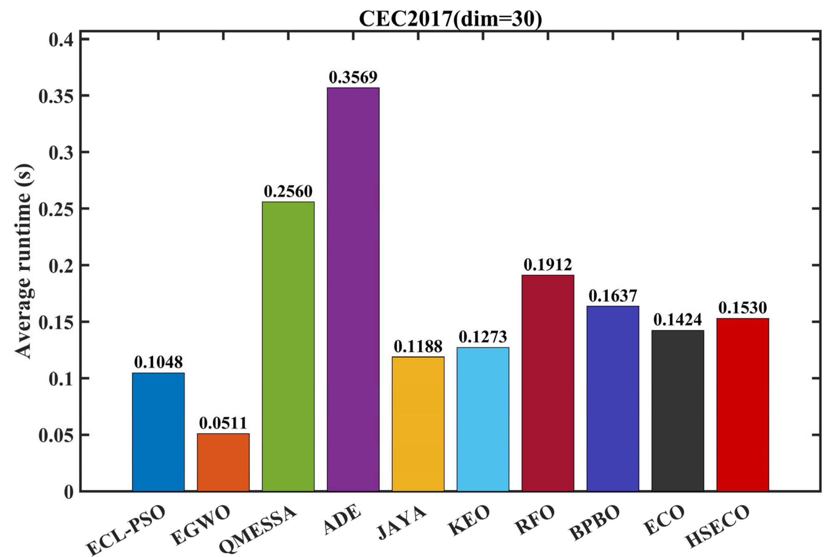
To further evaluate the computational efficiency of the proposed HSECO algorithm, the average runtime of all compared algorithms on the CEC2017 benchmark suite with 30 dimensions was recorded under the same experimental environment. The results are shown in Figure 9. All algorithms were executed using identical population size, maximum number of function evaluations, and independent runs, thereby ensuring fairness of the runtime comparison.

As shown in Figure 9, EGWO obtains the shortest average runtime of 0.0511 s, indicating that its search mechanism has relatively low computational overhead. ECL-PSO also shows high computational efficiency, with an average runtime of 0.1048 s. JAYA and KEO require 0.1188 s and 0.1273 s, respectively, suggesting that these algorithms maintain relatively simple update structures and low computational cost. ECO records an average runtime of 0.1424 s, while BPBO and RFO require 0.1637 s and 0.1912 s, respectively.

The proposed HSECO achieves an average runtime of 0.1530 s, which is slightly higher than that of the original ECO. This increase is reasonable because HSECO introduces additional mechanisms, including self-adaptive parameter evolution, multi-operator adaptive selection, and archive-assisted diversity maintenance. These components inevitably introduce extra computational operations, such as operator probability updating, archive maintenance, diversity monitoring, and partial reinitialization. However, the runtime increase compared with ECO is relatively small, increasing from 0.1424 s to 0.1530 s.

Compared with QMESSA and ADE, HSECO demonstrates better computational efficiency. QMESSA requires 0.2560 s, while ADE has the highest average runtime of 0.3569 s. This indicates that although HSECO incorporates multiple enhancement strategies, its computational burden remains moderate and does not lead to excessive runtime consumption. In particular, the adaptive mechanisms in HSECO are mainly based on lightweight vector operations and simple statistical updates, so the additional overhead is limited.

Overall, the runtime comparison demonstrates that HSECO achieves a favorable balance between computational cost and optimization performance. Although its runtime is slightly higher than that of ECO and several simpler algorithms, the improvement in convergence accuracy, robustness, and stability justifies this modest increase in computational cost. Therefore, HSECO can be considered computationally efficient and suitable for solving complex high-dimensional optimization problems.

4. UAV Three-Dimensional Path-Planning Model in Mountainous Terrain

Unmanned aerial vehicle (UAV) three-dimensional path-planning in mountainous terrain is a complex constrained optimization task. The goal is to find a safe, short, and smooth path from the start point to the end point under terrain collision avoidance, threat avoidance, and maneuverability constraints. Before establishing the mathematical model, we first describe the environmental characteristics, path structure, and optimization objectives in natural language.

The planning area includes rugged terrain, threatening regions, and altitude constraints. The path must be flyable, collision-free, and cost-minimized.

In complex mountainous environments, an unmanned aerial vehicle (UAV) is required to travel from a start point to a target point while ensuring terrain safety, threat avoidance, and smooth maneuvering. Due to the nonlinear terrain surface and the presence of threat regions, the path-planning task can be formulated as a constrained three-dimensional continuous optimization problem. In this section, the environment model, decision variables, path generation method, constraints, and objective function are presented in a unified mathematical formulation.

4.1. Three-Dimensional Mountain Environment Modeling

Consider a rectangular planning area in the horizontal plane:

$$\begin{array}{c}\mathsf{\Omega }=\{(x,y)\mid x\in [0,X_{max}],y\in [0,Y_{max}\left]\right\}\end{array}$$

(27)

where $X_{max}=200$ and $Y_{max}=200$ in the simulation. The terrain is represented by a height function:

$$\begin{array}{c}z=H(x,y)\end{array}$$

(28)

In the implemented model, the terrain height $H(x,y)$ is constructed by combining (i) an undulating base surface and (ii) a set of Gaussian-shaped mountains. Specifically, the Gaussian mountain component can be expressed as:

$$\begin{array}{c}{H}_m(x,y)={\displaystyle \sum _{i=1}^{n_h}}{h}_{i}exp\left(-{\displaystyle \frac{(x-x_i{)}^2}{a_i^2}}-{\displaystyle \frac{(y-y_i{)}^2}{b_i^2}}\right)\end{array}$$

(29)

where $n_h$ denotes the number of peaks, $(x_i,y_i)$ is the center of the $i$-th mountain, $h_i$ is the peak height, and $a_i,b_i$ control the slopes along the $x$- and $y$-directions, respectively. The final terrain height is defined as the maximum of the base undulation and the mountain superposition, which ensures prominent peaks are preserved:

$$\begin{array}{c}H(x,y)=max\{H_b(x,y),H_m(x,y)\}\end{array}$$

(30)

where $H_b(x,y)$ denotes the base oscillatory surface generated by trigonometric terms.

4.2. Threat Region Modeling

Assume there exist $n_T$ circular threat zones projected on the horizontal plane. The $k$-th threat zone is characterized by a center location $(x_k^T,y_k^T)$ and radius $R_k$. A UAV position $(x,y,z)$ is considered to violate the threat constraint if its horizontal distance to the threat center is smaller than the radius:

$$\begin{array}{c}\sqrt{(x-x_k^T{)}^2+(y-y_k^T{)}^2}<R_k,k=\mathrm{1,2},\dots ,n_T\end{array}$$

(31)

In other words, a feasible path must satisfy, for all points along the path:

$$\begin{array}{c}\sqrt{(x-x_k^T{)}^2+(y-y_k^T{)}^2}\ge R_k,\forall k\end{array}$$

(32)

In the simulation setup, one threat zone is used with center (50,140) and radius $R=30$.

4.3. Path Representation and Decision Variables

4.3.1. Start and End Points

The UAV start point and end point are defined in 3D space as:

$$\begin{array}{c}\mathbf{S}=(x_s,y_s,z_s),\mathbf{E}=(x_e,y_e,z_e)\end{array}$$

(33)

In the simulation, $\mathbf{S}=(\mathrm{0,0},20)$ $\mathrm{a}\mathrm{n}\mathrm{d}$ $\mathbf{E}=(\mathrm{200,200,40})$.

4.3.2. Control Nodes Between Start and End

To construct a smooth 3D flight path, $N$ intermediate control nodes are introduced between the start and end points:

$$\begin{array}{c}{\mathbf{P}}_i=(x_i,y_i,z_i),i=\mathrm{1,2},\dots ,N\end{array}$$

(34)

In the provided implementation, $N=2$. The key design choice is that the xxx-coordinates of the intermediate nodes are not optimized; instead, they are uniformly distributed along the straight-line direction from $\mathbf{S}$ to $\mathbf{E}$:

$$\begin{array}{c}{x}_i=x_s+{\displaystyle \frac{i}{N+1}}(x_e-x_s),i=\mathrm{1,2},\dots ,N\end{array}$$

(35)

This setting enforces a forward progression of the path and reduces the number of decision variables.

4.3.3. Optimization Vector Encoding

The optimization vector is constructed by concatenating the $y$-coordinates and the altitude offsets of the $N$ nodes:

$$\begin{array}{c}\mathbf{X}=[y_1,y_2,\dots ,y_N,\Delta z_1,\Delta z_2,\dots ,\Delta z_N]\end{array}$$

(36)

Hence, the dimension of the decision vector is:

$$\begin{array}{c}D=2N\end{array}$$

(37)

where $D=4$ when $N=2$.

The intermediate node altitude is defined relative to the terrain height to guarantee terrain-coupled modeling:

$$\begin{array}{c}{z}_i=H(x_i,y_i)+\Delta z_i\end{array}$$

(38)

where $\mathsf{\Delta }{z}_i$ is an optimization variable representing the extra height above the terrain at the iii-th control node.

4.4. Path Generation via Cubic Spline Interpolation

After constructing the control point set

$$\begin{array}{c}\mathcal{P}=\{\mathbf{S},{\mathbf{P}}_1,\dots ,{\mathbf{P}}_N,\mathbf{E}\}\end{array}$$

(39)

a continuous path is generated using cubic spline interpolation with a normalized parameter $t\in \left[\mathrm{0,1}\right]$. Let the discrete control points correspond to parameter values:

$$\begin{array}{c}{t}_j={\displaystyle \frac{j-1}{N+1}},j=\mathrm{1,2},\dots ,N+2\end{array}$$

(40)

where $j=1$ corresponds to $\mathbf{S}$ and $j=N+2$ corresponds to $\mathbf{E}$. The spline produces continuous functions:

$$\begin{array}{c}X(t),Y(t),Z(t)\end{array}$$

(41)

For numerical evaluation, the spline curve is sampled at $M$ evenly spaced points (in the code $M=200$):

$$\begin{array}{c}{t}_m={\displaystyle \frac{m-1}{M-1}},m=\mathrm{1,2},\dots ,M\end{array}$$

(42)

and the corresponding sampled path points are:

$$\begin{array}{c}{\mathbf{q}}_m=\left(\begin{array}{c}X(t_m),Y(t_m),Z(t_m)\end{array}\right)\end{array}$$

(43)

These sampled points are used for collision checking and objective evaluation.

4.5. Feasibility Constraints

To ensure safe flight, the candidate path must satisfy both terrain clearance and threat avoidance. The feasibility check is applied to all sampled points $q_m$.

4.5.1. Terrain Clearance Constraint

For each sampled point $(x_m,y_m,z_m).$, the altitude must be no lower than the terrain height at the same horizontal location:

$$\begin{array}{c}{z}_m\ge H(x_m,y_m),m=\mathrm{1,2},\dots ,M\end{array}$$

(44)

This constraint prevents the path from intersecting the terrain surface.

4.5.2. Threat Avoidance Constraint

For each threat zone $k$ and each sampled point, the horizontal distance must remain outside the threat radius:

$$\begin{array}{c}\sqrt{(x_m-x_k^T{)}^2+(y_m-y_k^T{)}^2}\ge R_k,\forall m,\forall k\end{array}$$

(45)

If any sampled point violates either constraint, the solution is labeled infeasible. In the implementation, infeasible solutions are penalized by assigning a very large fitness value:

$$\begin{array}{c}f(\mathbf{X})={10}^{33}\end{array}$$

(46)

which effectively eliminates them during optimization.

4.5.3. Variable Bounds

The decision variables are bounded to limit the search space:

$$\begin{array}{c}{y}_i\in [y_{min},y_{max}],\Delta z_i\in [\Delta z_{min},\Delta z_{max}]\end{array}$$

(47)

In the simulation:

$$\begin{array}{c}{y}_i\in \left[\mathrm{20,180}\right],\Delta z_i\in \left[\mathrm{0,50}\right]\end{array}$$

(48)

These bounds match the lower/upper bound vectors used in the optimizer.

4.6. Objective Function Construction

The path-planning objective integrates three criteria: total path length, altitude variation, and turning smoothness. The problem is formulated as a weighted single-objective minimization model.

It should be emphasized that the UAV path-planning problem considered in this study contains multiple performance responses, including path length, altitude variation, and turning smoothness. However, the proposed HSECO used in this paper is a single-objective optimizer. Therefore, these three responses are not optimized by a Pareto-dominance-based multi-objective framework. Instead, they are transformed into one scalar fitness function through a weighted-sum aggregation strategy. From the perspective of metaheuristic optimization, the final UAV path-planning model is therefore a single-objective constrained optimization problem.

4.6.1. Path Length Term

Using the sampled spline points $q_m$, the total 3D path length is computed by:

$$\begin{array}{c}L={\displaystyle \sum _{m=1}^{M-1}}\sqrt{(x_{m+1}-x_m{)}^2+(y_{m+1}-y_m{)}^2+(z_{m+1}-z_m{)}^2}\end{array}$$

(49)

This term encourages short and efficient trajectories.

4.6.2. Height Variation Term

To discourage excessive altitude fluctuation, the height variation is measured by the deviation of sampled altitudes from their mean:

$$\begin{array}{c}{\displaystyle \genfrac{}{}{0pt}{}{\overline{z}=\frac{1}{M}{\displaystyle {\sum }_{m=1}^M}{z}_m}{H_v={\displaystyle {\sum }_{m=1}^M}|z_m-\overline{z}|}}\end{array}$$

(50)

A smaller $H_v$ implies a more stable altitude profile.

4.6.3. Turning Smoothness Term

Let the discrete direction vectors along the path be:

$$\begin{array}{c}{\mathbf{v}}_m={\mathbf{q}}_{m+1}-{\mathbf{q}}_m,m=\mathrm{1,2},\dots ,M-1\end{array}$$

(51)

The cosine of the turning angle between consecutive segments is:

$$\begin{array}{c}{C}_m={\displaystyle \frac{{\mathbf{v}}_m\cdot {\mathbf{v}}_{m+1}}{\parallel {\mathbf{v}}_m\parallel \parallel {\mathbf{v}}_{m+1}\parallel }},m=\mathrm{1,2},\dots ,M-2\end{array}$$

(52)

To penalize sharp turns, the turning cost is defined as:

$$\begin{array}{c}T={\displaystyle \sum _{m=1}^{M-2}}(cos\varphi -C_m)\end{array}$$

(53)

where $\varphi =\pi /2$ is a reference angle used in the implementation. When the path is smoother, $C_m$ tends to be closer to 1, making $(\mathrm{c}\mathrm{o}\mathrm{s} \varphi -C_m)$ smaller (or more negative), thus improving the objective.

4.7. Final Optimization Model

The overall fitness function is defined as a weighted sum of the three components:

$$\begin{array}{c}\underset{\mathbf{X}}{min }f (\mathbf{X})=w_{1}L+w_2{H}_v+w_{3}T\end{array}$$

(54)

where $w_1,w_2,w_3$ are nonnegative weights satisfying $w_1+w_2+w_3=1$. In the simulation, the weights are set as:

$$\begin{array}{c}{w}_1=0.5,w_2=0.3,w_3=0.2\end{array}$$

(55)

The weights in Equation (54) reflect the relative importance assigned to the three path-quality responses. In this study, the path length is assigned the largest weight because flight distance is directly related to energy consumption and mission efficiency. The altitude variation term is assigned a moderate weight to encourage stable flight and avoid unnecessary vertical maneuvers. The turning smoothness term is also considered to reduce sharp turns and improve trajectory feasibility. To reduce the subjectivity caused by manual weight assignment, the three weights were selected according to the following principles: first, all objective components were normalized or evaluated under comparable scales before aggregation; second, the weight values were determined based on the engineering priority of UAV path-planning, where path efficiency, flight stability, and smoothness are considered in descending order of importance; third, additional trial experiments were conducted to ensure that no single response completely dominated the final fitness value. Therefore, the adopted weight setting represents a practical trade-off among path length, altitude stability, and turning smoothness rather than an arbitrary subjective choice.

For clarity, the adopted weights do not imply a Pareto-based multi-objective optimization process. They only serve as preference coefficients for converting multiple responses into a scalar objective value. Different weight settings may lead to different preference-oriented paths, and a full sensitivity analysis of weight combinations will be considered in future work.

Finally, the complete constrained optimization model can be written as:

$$\begin{array}{c}minf(\mathbf{X})=0.5L+0.3H_v+0.2T\hfill \\ s.t.z_m\ge H(x_m,y_m),m=\mathrm{1,2},\dots ,M\hfill \\ \hspace{1em}\hspace{1em} \sqrt{(x_m-x_k^T{)}^2+(y_m-y_k^T{)}^2}\ge R_k,\forall m,\forall k\hfill \\ \hspace{1em}\hspace{1em} y_i\in \left[\mathrm{20,180}\right],i=\mathrm{1,2},\dots ,N\hfill \\ \hspace{1em}\hspace{1em} \Delta z_i\in \left[\mathrm{0,50}\right],i=\mathrm{1,2},\dots ,N\hfill \end{array}$$

(56)

This model is a nonlinear constrained optimization problem in continuous space. Because the terrain function $H(x,y)$ is non-convex and the threat constraint introduces discontinuous feasible regions, metaheuristic optimizers are suitable to search for high-quality feasible paths.

4.8. Experimental Setup and Results

To further verify the practical applicability and problem-solving capability of HSECO in real-world engineering optimization tasks, a three-dimensional UAV path-planning problem in mountainous terrain was adopted as an application scenario. HSECO and nine comparison algorithms were applied to this constrained nonlinear optimization problem. The performance of each algorithm was comprehensively evaluated from multiple perspectives, including the generated three-dimensional flight trajectories, planar top-view paths, fitness convergence curves, and quantitative statistical indicators. Specifically, the evaluation criteria considered path feasibility, optimality, smoothness, and computational efficiency, thereby providing an integrated assessment of the optimization performance of HSECO in practical engineering contexts.

The algorithm parameter settings are the same as those described in the previous section. The experimental results are illustrated in Figure 10, Figure 11 and Figure 12 and summarized in

Table 7. Statistics of drone path-planning simulation results.

Algorithm	Mean	Std	Best	Worst	Median	Run Time	Friedman	Friedman Rank
ECL-PSO	287.95	25.98	275.06	358.88	275.06	32.63	3.37	2
EGWO	333.05	31.96	275.06	409.57	337.85	31.10	7.87	9
QMESSA	296.75	24.78	275.06	365.87	293.43	33.72	5.20	4
ADE	306.90	33.30	275.06	357.38	298.97	28.75	6.03	5
JAYA	381.07	34.08	327.21	476.39	376.39	30.38	9.37	10
KEO	336.03	38.06	275.06	409.72	349.47	39.39	7.20	8
RFO	308.29	36.31	275.06	409.56	311.64	35.29	4.43	3
BPBO	313.86	38.06	275.23	413.80	301.20	28.19	7.03	7
ECO	321.08	49.49	275.07	453.73	311.85	31.22	6.77	6
HSECO	283.80	23.52	275.05	362.12	275.06	31.41	3.03	1

.

From the three-dimensional flight trajectory in Figure 10, it can be observed that the path generated by HSECO is the smoothest and most reasonable among all ten algorithms. Starting from the initial point (0, 0, 20), the trajectory steadily avoids terrain elevations and the circular threat region labeled as No. 1 (centered at (50, 140) with a radius of 30). Throughout the flight from the start to the destination (200, 200, 40), the path maintains a safe clearance from the terrain while avoiding unnecessary altitude fluctuations. The overall trajectory exhibits a smooth arc-like shape, which conforms well to the maneuverability constraints of fixed-wing UAVs.

In contrast, although the paths generated by ECL-PSO and KEO successfully connect the start and end points, they pass close to the peaks of mountainous terrain in certain mid-course segments, resulting in insufficient safety margins. The trajectory obtained by EGWO shows a sharp altitude drop around x = 100 followed by a rapid climb, which is impractical for real flight operations. The paths generated by ADE and QMESSA are generally reasonable but contain multiple minor fluctuations in the latter half, indicating suboptimal smoothness. BPBO introduces unnecessary detours near the threat region, increasing the overall path length. The trajectory produced by the original ECO exhibits abrupt altitude changes in the mid-to-late stages, dropping from approximately 40 m to near-ground level and then rapidly climbing, which compromises flight safety and violates energy-efficient flight principles. The paths generated by JAYA and RFO contain numerous sharp turns and zigzag patterns, resulting in disordered trajectories that are nearly infeasible for practical flight. Notably, portions of the RFO trajectory even fall below the terrain surface, directly violating terrain-avoidance constraints.

The top-view path-planning results in Figure 11 further illustrate the horizontal navigation strategies of different algorithms. HSECO produces the most direct and smooth planar path, forming an approximately smooth curve from the start to the destination. Within the interval x = 50 to x = 100, the path bypasses the threat region from the right side with a curvature, achieving a good balance between path length and safety distance without unnecessary detours or excessive proximity to the threat center.

The planar path generated by ECL-PSO is also relatively reasonable; however, its curvature around the threat region is slightly larger than that of HSECO, leading to a longer projected distance. The path generated by KEO exhibits a slight “S”-shaped deviation after bypassing the threat region. The paths of ADE, QMESSA, and BPBO deviate from the optimal direction in certain segments, particularly BPBO, which shows hesitation and oscillation before reaching the threat region, resulting in locally tortuous paths. The planar trajectories of ECO and EGWO are more irregular, with ECO exhibiting a sharp turn near x = 80, while EGWO presents a zigzag pattern with multiple unnecessary directional adjustments, making it difficult to maintain stable flight. JAYA and RFO produce the most disordered paths; JAYA’s trajectory appears almost randomly distributed, with some solutions deviating significantly from the general direction between the start and end points, while RFO lacks overall consistency and contains multiple sharp turns. These observations indicate that JAYA and RFO lack effective guidance mechanisms when dealing with constrained path-planning problems.

The convergence curves in Figure 12 further reveal the dynamic optimization behaviors of the algorithms. HSECO exhibits a significantly lower convergence curve from the initial stage, rapidly decreasing to a low level within approximately 50 iterations, and then continuing a steady decline until convergence around 250 iterations, without any noticeable stagnation or oscillation. This smooth and continuous descent validates the effectiveness of the proposed self-adaptive parameter evolution and Archive-Assisted Diversity Maintenance Strategy in handling constrained optimization problems.

ECL-PSO demonstrates the second-fastest convergence, reaching near convergence after approximately 100 iterations, although its final fitness value is about four units higher than that of HSECO. The convergence curves of RFO and KEO decrease rapidly in the early stage but exhibit multiple fluctuations in the later stages, indicating insufficient stability. QMESSA and ADE show relatively stable convergence processes; however, their convergence speeds are noticeably slower than that of HSECO, and their final accuracies are inferior. BPBO exhibits a slow convergence trend, stabilizing only after approximately 300 iterations, indicating low efficiency.

The convergence behavior of the original ECO is particularly noteworthy. Although it shows some improvement within the first 50 iterations, the curve subsequently stagnates almost completely, with no further optimization even after 200 iterations. This indicates that ECO is highly prone to being trapped in local optima when applied to constrained path-planning problems and lacks effective escape mechanisms. This observation is consistent with the population diversity analysis in Section 3.2.4, where ECO exhibits rapid loss of diversity in the early stage, leading to exhausted search capability in later iterations. The convergence curve of JAYA remains nearly flat throughout the process, indicating almost no effective optimization, which suggests a significant mismatch between its search mechanism and terrain-constrained path-planning problems.

The quantitative results in Table 7 provide a more systematic and precise evaluation of algorithm performance. HSECO achieves the best results in five out of six evaluation metrics. Specifically, in terms of mean cost, HSECO ranks first with a value of 283.80, followed by ECL-PSO (287.95) and RFO (308.29), with gaps of approximately 4.15 and 24.5, respectively. The original ECO records a mean cost of 321.08, which is 37.28 higher than HSECO, corresponding to a relative difference of 13.1%. JAYA performs the worst, with a mean cost of 381.07, approximately 1.34 times that of HSECO, highlighting the superior solution accuracy of HSECO.

In terms of standard deviation, HSECO achieves the smallest value of 23.52, indicating the strongest robustness and the least variation across independent runs. ECO exhibits a much larger standard deviation of 49.49, approximately 2.1 times that of HSECO, indicating high sensitivity to initial populations and randomness. Although JAYA has a lower standard deviation (34.08) than ECO, its significantly higher mean cost suggests that its “stability” is achieved at the expense of consistently poor solutions.

Regarding the best cost, HSECO achieves a value of 275.05, which is very close to those of ECL-PSO, EGWO, QMESSA, KEO, RFO, and ECO (all within the range of 275.05 to 275.07). This indicates that multiple algorithms are capable of locating the vicinity of the global optimum. However, HSECO attains the theoretically best value and maintains a much smaller gap between its mean and best values (8.75) compared to ECO (46.01), further demonstrating its superior stability.

In terms of worst cost, HSECO records 362.12, which is not the best (ADE achieves 357.38) but is significantly better than ECO (453.73) and JAYA (476.39). This indicates that even under unfavorable conditions, HSECO can maintain a reasonable optimization quality, whereas ECO and JAYA may fail in certain runs. For the median cost, HSECO achieves 275.06, which is nearly identical to its best cost, indicating that more than half of the independent runs reach near-optimal solutions. In contrast, ECO has a median cost of 311.85, far from its best value, suggesting that most of its runs deviate significantly from the optimum.

In terms of runtime, HSECO requires 31.41 s, representing a moderate computational cost. BPBO (28.19 s) and ADE (28.75 s) are slightly faster, while ECL-PSO requires 32.63 s. Although HSECO incurs slightly higher computational cost than BPBO and ADE, its significantly superior accuracy and robustness justify this overhead. KEO has the longest runtime (39.39 s) but does not achieve competitive accuracy.

According to the Friedman mean rank results, HSECO ranks first with a score of 3.03, followed by ECL-PSO (3.37), with a gap of 0.34. RFO ranks third with 4.43, while EGWO (7.87) and JAYA (9.37) occupy the bottom positions. The original ECO ranks sixth with a score of 6.77, which is 3.74 positions behind HSECO. This statistical result further confirms the overall superiority of HSECO across multiple metrics and repeated runs.

In summary, HSECO demonstrates significantly superior overall performance compared to nine competing algorithms in the three-dimensional UAV path-planning problem over mountainous terrain. The generated trajectories are the smoothest in 3D space, the most direct in planar projection, and the safest in terms of terrain and threat avoidance, while also achieving the fastest convergence speed, lowest final cost, and strongest robustness. The quantitative results consistently validate these advantages across multiple metrics, including mean cost, standard deviation, best cost, median, worst cost, and Friedman ranking. These findings confirm the strong engineering applicability of HSECO in constrained nonlinear continuous optimization problems and further highlight the effectiveness and promising potential of the proposed hybrid enhancement framework in complex real-world scenarios.

5. Pressure Vessel Design Problem

To further validate the effectiveness and generality of HSECO in practical constrained engineering optimization problems, the classical pressure vessel design problem is selected as an additional real-world application case. The objective of this problem is to minimize the manufacturing cost of a cylindrical pressure vessel, subject to multiple nonlinear constraints involving design variables such as shell thickness, head thickness, inner radius, and the length of the cylindrical section. Due to its narrow feasible region, complex constraints, and the presence of multiple local optima, this problem has been widely used to evaluate the search capability and convergence stability of optimization algorithms in constrained engineering scenarios. Therefore, testing HSECO on this problem provides a more comprehensive assessment of its performance in real-world optimization tasks.

The pressure vessel design problem is a well-known constrained optimization task widely encountered in mechanical and chemical engineering. Its objective is to minimize the overall manufacturing cost of a cylindrical pressure vessel while satisfying a series of structural strength, volumetric, and geometric constraints. As illustrated in Figure 13, the vessel is composed of a cylindrical shell and two hemispherical end caps.

The decision variables include the shell thickness $T_s$, the head thickness $T_h$, the inner radius $R$, and the length of the cylindrical section $L$. The total production cost, which accounts for material usage, forming, and welding operations, can be expressed by the following objective function:

$$\begin{array}{c}minf(\mathbf{x})=0.6224T_{s}RL+1.7781T_h{R}^2+3.1661T_s^{2}L+19.84T_s^{2}R\end{array}$$

(57)

The constraints are derived from both mechanical strength requirements and geometric limitations. To guarantee that the vessel can endure internal pressure safely, the thicknesses of the shell and head must meet the following conditions:

$$\begin{array}{c}{\displaystyle \genfrac{}{}{0pt}{}{\begin{array}{c}{g}_1\left(\mathbf{x}\right)=0.0193R-T_s\le 0\\ g_2\left(\mathbf{x}\right)=0.00954R-T_h\le 0\end{array}}{\begin{array}{c}{g}_3(\mathbf{x})=\pi R^{2}L+\frac{4}{3}\pi R^3-1296000\le 0\\ g_4(\mathbf{x})=L-240\le 0\end{array}}}\end{array}$$

(58)

The allowable ranges of the design variables are given as:

$$\begin{array}{c}1\le T_s,T_h\le \mathrm{99,10}\le R,L\le 200\end{array}$$

(59)

The experimental results are presented in Figure 14 and

Table 8. Statistical results obtained by different algorithms for the pressure vessel design problem.

Algorithm	Best	Mean	Std	Friedman Rank	Rank
ECL-PSO	5.90499E+03	6.22907E+03	3.04130E+02	5.63	5
EGWO	5.88534E+03	6.09256E+03	3.29771E+02	4.00	3
QMESSA	5.88533E+03	6.52641E+03	6.32587E+02	5.93	6
ADE	5.92391E+03	6.62530E+03	5.27472E+02	7.47	9
JAYA	5.96689E+03	6.29920E+03	2.26596E+02	6.40	7
KEO	6.01253E+03	6.32209E+03	2.66476E+02	6.47	8
RFO	6.06230E+03	6.95310E+03	3.96311E+02	8.87	10
BPBO	5.88534E+03	5.93444E+03	5.65367E+01	2.87	2
ECO	5.88731E+03	6.18165E+03	2.81294E+02	5.40	4
HSECO	5.88533E+03	5.90819E+03	4.95957E+01	1.97	1

.

Figure 14 presents the statistical comparison results of different algorithms on the pressure vessel design problem, illustrating the distribution of objective function values obtained from multiple independent runs. It can be clearly observed that the results of HSECO are the most concentrated, with very few outliers, indicating a high level of consistency across runs. In contrast, algorithms such as EGWO, QMESSA, and RFO exhibit more dispersed distributions with larger variability, suggesting lower stability when handling complex constraints. Similarly, the results of JAYA and ADE are less concentrated, with some runs deviating significantly from the optimal solution. Overall, Figure 14 demonstrates that HSECO achieves superior convergence consistency and robustness on this problem.

Table 8 further validates these observations from a quantitative perspective. In terms of the best value, HSECO achieves 5.88533E+03, which is comparable to the best results obtained by EGWO, QMESSA, and BPBO, indicating that multiple algorithms are capable of approaching the theoretical optimum. However, in terms of the mean value, HSECO significantly outperforms all comparison algorithms with a value of 5.90819E+03, while EGWO, ECL-PSO, and ECO achieve 6.09256E+03, 6.22907E+03, and 6.18165E+03, respectively, and RFO records a much higher mean value of 6.95310E+03. These results indicate that although some algorithms may occasionally obtain competitive solutions in single runs, their overall performance is far less stable than that of HSECO, highlighting the superior reliability of HSECO across repeated runs.

In terms of standard deviation, HSECO achieves the lowest value of 4.95957E+01 among all algorithms, which is significantly smaller than those of EGWO (3.29771E+02), QMESSA (6.32587E+02), and ECO (2.81294E+02). This demonstrates that the optimization results of HSECO are minimally affected by initial population settings and stochastic factors, reflecting strong robustness. Finally, according to the Friedman mean rank results, HSECO ranks first with a score of 1.97, significantly outperforming BPBO (2.87) and EGWO (4.00), while RFO and ADE rank tenth and ninth, respectively. This further confirms the overall superiority of HSECO on the pressure vessel design problem.

In summary, through experimental validation on the classical pressure vessel design problem, HSECO demonstrates superior performance over all comparison algorithms in terms of solution quality, mean performance, stability, and overall ranking. These findings strongly confirm its practical value and excellent performance in complex nonlinear constrained optimization scenarios.

6. Summary and Prospect

This paper proposes a Hybrid Strategy Enhanced Educational Competition Optimizer (HSECO) to address the limitations of the original ECO when solving high-dimensional and complex optimization problems, including fixed stage scheduling, limited update mechanisms, and insufficient diversity preservation. A unified hybrid framework is constructed by integrating three complementary strategies: a Self-Adaptive Parameter Evolution Strategy (SAPES), a Multi-Operator Adaptive Selection Strategy (MOASS), and an Archive-Assisted Diversity Maintenance Strategy (AADMS).

Extensive experimental evaluations conducted on the CEC2017, CEC2020, and CEC2022 benchmark suites demonstrate that HSECO significantly outperforms nine State-of-the-Art metaheuristic algorithms in terms of optimization accuracy, convergence speed, and robustness. Statistical analyses using the Wilcoxon rank-sum test and the Friedman average ranking test further confirm that the performance improvements achieved by HSECO are statistically significant rather than the result of random variation.

Moreover, HSECO was applied to a three-dimensional UAV path-planning problem in mountainous terrain. In this application, the multiple path-quality responses, including path length, altitude variation, and turning smoothness, were aggregated into a single weighted fitness function. Therefore, the UAV problem was solved as a single-objective constrained optimization problem rather than a Pareto-based multi-objective optimization problem. The experimental results demonstrate that HSECO can generate safer, smoother, and lower-cost flight trajectories while maintaining stable convergence behavior.

Despite the promising performance of HSECO, several limitations should be acknowledged. According to the No Free Lunch (NFL) theorem, no optimization algorithm can perform optimally across all problem domains. Although HSECO demonstrates strong performance on high-dimensional and complex benchmark functions, its advantage may be less significant for simple unimodal problems. In addition, the introduction of multiple adaptive strategies inevitably increases the computational overhead compared with simpler algorithms. Although the runtime analysis indicates that this increase remains moderate, it may still affect efficiency in time-sensitive applications. Furthermore, the performance of HSECO may still depend on the selection of certain control parameters, although the sensitivity analysis demonstrates acceptable robustness within a reasonable range.

Despite these limitations, several directions remain for further investigation. First, a multi-objective extension of HSECO could be developed to address trade-off optimization problems, such as multi-objective path-planning and multi-performance engineering design. Second, incorporating dynamic environment modeling mechanisms would enable the algorithm to handle time-varying optimization scenarios. Third, integrating deep learning or reinforcement learning techniques for higher-level operator scheduling may further enhance adaptive decision-making capability. In addition, scalability analysis for large-scale ultra-high-dimensional optimization problems remains an important research topic.

Furthermore, although HSECO has been compared with several representative and State-of-the-Art metaheuristic algorithms, the current study does not include some highly competitive adaptive differential evolution frameworks and top-performing algorithms from recent CEC competitions, such as SHADE and L-SHADE variants. Therefore, the generalization capability and competitiveness of HSECO against these advanced adaptive optimization frameworks still require further investigation. Future work will include more extensive comparative studies with advanced adaptive differential evolution algorithms and top-ranking CEC competition optimizers to provide a more comprehensive evaluation of HSECO under different optimization scenarios.

In addition, although the UAV path-planning experiment demonstrates the feasibility of HSECO in constrained engineering optimization, the current UAV scenario remains relatively simplified compared with real-world applications. We have explicitly acknowledged this limitation and added corresponding discussions in the conclusion section. Future work will focus on extending HSECO to more complex UAV path-planning environments involving multiple dynamic threat zones, terrain-following constraints, kinematic limitations, and dynamic real-time path replanning problems, thereby further enhancing its practical engineering applicability.

Through continued theoretical development and practical expansion, HSECO is expected to demonstrate broader application potential in intelligent manufacturing, energy optimization scheduling, autonomous-driving path-planning, and cooperative control of unmanned systems.

References

1. Fu, Y.; Liu, D.; Chen, J.; He, L. Secretary bird optimization algorithm: A new metaheuristic for solving global optimization problems. Artif. Intell. Rev. 2024, 57, 123. [Google Scholar] [CrossRef]
2. Di Puglia Pugliese, L.; Guerriero, F.; Mitton, N. Optimizing wireless sensor networks deployment with coverage and connectivity requirements. Ann. Oper. Res. 2025, 346, 1997–2008. [Google Scholar] [CrossRef]
3. Yu, M.Y.; Du, J.; Xu, X.X.; Xu, J.; Jiang, F.; Fu, S.W.; Zhang, J.; Liang, A.K. A multi-strategy enhanced Dung Beetle Optimization for real-world engineering problems and UAV path planning. Alex. Eng. J. 2025, 118, 406–434. [Google Scholar] [CrossRef]
4. Yu, M.; Xu, J.; Liang, W.; Qiu, Y.; Bao, S.; Tang, L. Improved multi-strategy adaptive Grey Wolf Optimization for practical engineering applications and high-dimensional problem solving. Artif. Intell. Rev. 2024, 57, 277. [Google Scholar] [CrossRef]
5. Yu, M.; Yang, H.; Wei, X.; Fu, S.; Xu, J.; Zhang, J. Carbon Footprint Efficiency Ratio: A Unified Indicator for Green Evaluation of Evolutionary Algorithms. IEEE Trans. Emerg. Top. Comput. Intell. 2026; early access.
6. Kennedy, J.; Eberhart, R. Particle swarm optimization. In Proceedings of ICNN’95—International Conference on Neural Networks; Perth, WA, Australia, 27 November–1 December 1995, IEEE: New York, NY, USA, 1995; Volume 4, pp. 1942–1948. [Google Scholar]
7. Dorigo, M.; Birattari, M.; Stützle, T. Ant Colony Optimization. In Computational Intelligence Magazine; IEEE: New York, NY, USA, 2006; Volume 1, pp. 28–39. [Google Scholar]
8. Karaboga, D. Artificial bee colony algorithm. Scholarpedia 2010, 5, 6915. [Google Scholar] [CrossRef]
9. Mirjalili, S.; Mirjalili, S.M.; Lewis, A. Grey Wolf Optimizer. Adv. Eng. Softw. 2014, 69, 46–61. [Google Scholar] [CrossRef]
10. Mirjalili, S.; Lewis, A. The Whale Optimization Algorithm. Adv. Eng. Softw. 2016, 95, 51–67. [Google Scholar] [CrossRef]
11. Cao, L.; Wei, Q. SZOA: An Improved Synergistic Zebra Optimization Algorithm for Microgrid Scheduling and Management. Biomimetics 2025, 10, 664. [Google Scholar] [CrossRef]
12. Zhang, Y.; Wang, J.; Zhang, X.; Wang, B. ACPOA: An Adaptive Cooperative Pelican Optimization Algorithm for Global Optimization and Multilevel Thresholding Image Segmentation. Biomimetics 2025, 10, 596. [Google Scholar] [CrossRef]
13. Liu, Z.; Han, F.; Ling, Q.; Han, H.; Jiang, J. Constraint-Pareto Dominance and Diversity Enhancement Strategy based Evolutionary Algorithm for Solving Constrained Multiobjective Optimization Problems. IEEE Trans. Evol. Comput. 2025, 29, 2771–2784. [Google Scholar] [CrossRef]
14. Manoharan, P.; Jangir, P.; Kumar, S.; Ravichandran, S.; Alhelou, H.H.; Abualigah, L.; Yildiz, A.R.; Mirjalil, S. A New Arithmetic Optimization Algorithm for Solving Real-World Multiobjective CEC-2021 Constrained Optimization Problems: Diversity Analysis and Validations. IEEE Access 2021, 9, 84263–84295. [Google Scholar] [CrossRef]
15. Coello, C.A.C.; Lechuga, M.S. MOPSO: A proposal for multiple objective particle swarm optimization. In Proceedings of the 2002 Congress on Evolutionary Computation, CEC’02 (Cat. No.02TH8600), Honolulu, HI, USA, 12–7 May 2003; Volume 2, pp. 1051–1056. [Google Scholar]
16. Mirjalili, S.; Saremi, S.; Mirjalili, S.M.; Coelho, L.D.S. Multi-objective grey wolf optimizer: A novel algorithm for multi-criterion optimization. Expert Syst. Appl. 2016, 47, 106–119. [Google Scholar] [CrossRef]
17. He, L.; Li, W.; Chiong, R.; Abedi, M.; Cao, Y.; Zhang, Y. Optimising the job-shop scheduling problem using a multi-objective Jaya algorithm. Appl. Soft Comput. 2021, 111, 107654. [Google Scholar] [CrossRef]
18. Zhang, Q.; Li, H. MOEA/D: A Multiobjective Evolutionary Algorithm Based on Decomposition. IEEE Trans. Evol. Comput. 2007, 11, 712–731. [Google Scholar] [CrossRef]
19. Deb, K.; Pratap, A.; Agarwal, S.; Meyarivan, T. A fast and elitist multiobjective genetic algorithm: NSGA-II. IEEE Trans. Evol. Comput. 2002, 6, 182–197. [Google Scholar] [CrossRef]
20. Peng, Y.; Gu, S.W.; Liang, Y.B.; Ouyang, K.C.; Li, Y.L.; Wang, K.; Wu, G.H.; Fan, C.J. Wave Optics Optimizer: A novel meta-heuristic algorithm for engineering optimization. Commun. Nonlinear Sci. Numer. Simul. 2025, 152, 109337. [Google Scholar] [CrossRef]
21. Abedinpourshotorban, H.; Shamsuddin, S.M.; Beheshti, Z.; Jawawi, D.N.A. Electromagnetic field optimization: A physics-inspired metaheuristic optimization algorithm. Swarm Evol. Comput. 2015, 26, 8–22. [Google Scholar] [CrossRef]
22. Heidari, A.A.; Mirjalili, S.; Faris, H.; Aljarah, I.; Mafarja, M.; Chen, H. Harris hawks optimization: Algorithm and applications. Future Gener. Comput. Syst. 2019, 97, 849–872. [Google Scholar] [CrossRef]
23. Xue, J.; Shen, B. A novel swarm intelligence optimization approach: Sparrow search algorithm. Syst. Sci. Control. Eng. 2020, 8, 22–34. [Google Scholar] [CrossRef]
24. Xue, J.; Shen, B. Dung beetle optimizer: A new meta-heuristic algorithm for global optimization. J. Supercomput. 2023, 79, 7305–7336. [Google Scholar] [CrossRef]
25. Fu, S.; Li, K.; Huang, H.; Ma, C.; Fan, Q.; Zhu, Y. Red-billed blue magpie optimizer: A novel metaheuristic algorithm for 2D/3D UAV path planning and engineering design problems. Artif. Intell. Rev. 2024, 57, 134. [Google Scholar] [CrossRef]
26. Wang, J.; Shang, Z. Traffic jam optimizer: A novel swarm-based metaheuristic algorithm for solving global optimization problems. Appl. Math. Model. 2026, 150, 116410. [Google Scholar] [CrossRef]
27. Yu, M.Y.; Yang, H.R.; Zhang, J.Q.; Ouyang, K.C.; Fu, S.W.; Tan, P.L.; Jiang, F.; Xu, J. Bounty hunter optimizer: A novel metaheuristic with an application to multi-UAV mobile edge computing and path planning. Knowl.-Based Syst. 2026, 341, 115836. [Google Scholar] [CrossRef]
28. Wang, T.-L.; Gu, S.-W.; Liu, R.-J.; Chen, L.-Q.; Wang, Z.; Zeng, Z.-Q. Cuckoo catfish optimizer: A new meta-heuristic optimization algorithm. Artif. Intell. Rev. 2025, 58, 326. [Google Scholar] [CrossRef]
29. Talatahari, S.; Bayazidi, H.; Sareh, P. Philosophical proposition optimizer (ΦPO): An epistemology-inspired algorithm for numerical optimization. Artif. Intell. Rev. 2025, 58, 1–70. [Google Scholar] [CrossRef]
30. Zhao, S.; Zhang, T.; Ma, S.; Wang, M. Sea-horse optimizer: A novel nature-inspired meta-heuristic for global optimization problems. Appl. Intell. 2022, 53, 11833–11860. [Google Scholar] [CrossRef]
31. Wang, R.B.; Hu, R.B.; Geng, F.D.; Xu, L.; Chu, S.C.; Pan, J.S.; Meng, Z.Y.; Mirjalili, S. The Animated Oat Optimization Algorithm: A nature-inspired metaheuristic for engineering optimization and a case study on Wireless Sensor Networks. Knowl.-Based Syst. 2025, 318, 113589. [Google Scholar] [CrossRef]
32. Wei, J.; Gu, Y.; Lu, B.; Cheong, N. RWOA: A novel enhanced whale optimization algorithm with multi-strategy for numerical optimization and engineering design problems. PLoS ONE 2025, 20, e0320913. [Google Scholar] [CrossRef]
33. Wang, Z.; Ye, X.; Jiang, G.; Yi, Y. Improved Zebra Optimization Algorithm with Multi Strategy Fusion and Its Application in Robot Path Planning. Biomimetics 2025, 10, 354. [Google Scholar] [CrossRef]
34. Yu, M.Y.; Zhang, J.Q.; Yu, L.; Yang, H.R.; Lu, H.T.; Wei, X.J.; Xu, J. Alzheimer’s disease brain image segmentation using multi-feature fusion in 3D Rényi entropy model and quantum hybrid optimization. Artif. Intell. Rev. 2026, 59, 95. [Google Scholar] [CrossRef]
35. Wolpert, D.H.; Macready, W.G. No free lunch theorems for optimization. IEEE Trans. Evol. Comput. 1997, 1, 67–82. [Google Scholar] [CrossRef]
36. Wang, X.; Snášel, V.; Mirjalili, S.; Pan, J.-S. MAAPO: An innovative membrane algorithm based on artificial protozoa optimizer for multilevel threshold image segmentation. Artif. Intell. Rev. 2025, 58, 1–40. [Google Scholar] [CrossRef]
37. Tang, X.J.; Lian, J.J.; Ma, L.; Wu, X.C.; Zhong, R.; Zhang, Y.J.; Chen, H.L. IECO: An improved educational competition optimizer for state-of-the-art engineering optimization. J. Big Data 2025, 12, 200. [Google Scholar] [CrossRef]
38. Çelik, E. A powerful variant of symbiotic organisms search algorithm for global optimization. Eng. Appl. Artif. Intell. 2020, 87, 103294. [Google Scholar] [CrossRef]
39. Çelik, E.; Houssein, E.H.; Abdel-Salam, M.; Oliva, D.; Tejani, G.G.; Öztürk, N.; Sharma, S.K.; Baljon, M. Novel distance-fitness learning scheme for ameliorating metaheuristic optimization. Eng. Sci. Technol. Int. J. 2025, 65, 102053. [Google Scholar] [CrossRef]
40. Çelik, E. IEGQO-AOA: Information-exchanged gaussian arithmetic optimization algorithm with quasi-opposition learning. Knowl.-Based Syst. 2023, 260, 110169. [Google Scholar] [CrossRef]
41. Lian, J.B.; Zhu, T.; Ma, L.; Wu, X.C.; Heidari, A.A.; Chen, Y.; Chen, H.L.; Hui, G.H. The educational competition optimizer. Int. J. Syst. Sci. 2024, 55, 3185–3222. [Google Scholar] [CrossRef]
42. Tang, W.; Shi, S.; Lu, Z.; Lin, M.; Cheng, H. EDECO: An Enhanced Educational Competition Optimizer for Numerical Optimization Problems. Biomimetics 2025, 10, 176. [Google Scholar] [CrossRef]
43. Qian, C.; Cai, X. An efficient social-driven educational competition optimizer for numerical optimization. Clust. Comput. 2025, 28, 1–40. [Google Scholar] [CrossRef]
44. Li, S.; Luo, J. Comprehensive Learning-Enhanced Educational Competition Optimizer for Numerical Optimization and Reservoir Production Optimization. Biomimetics 2026, 11, 111. [Google Scholar] [CrossRef]
45. Zhao, B.; Yang, X.; Lee, H.; Dong, B. An improved educational competition optimizer with multi-covariance learning operators for global optimization problems. Clust. Comput. 2025, 28, 964. [Google Scholar] [CrossRef]
46. Gupta, S.; Gautam, K. Enhanced cooperative learning and local search integrated particle swarm optimization for global optimization and coverage enhancement in wireless sensor network. Swarm Evol. Comput. 2026, 100, 102262. [Google Scholar] [CrossRef]
47. Iraninezhad, R.; Asheghi, R.; Ahmadi, H. A new enhanced grey wolf optimizer to improve geospatially subsurface analyses. Model. Earth Syst. Environ. 2025, 11, 1–16. [Google Scholar] [CrossRef]
48. Wu, R.; Huang, H.S.; Wei, J.A.; Ma, C.; Zhu, Y.W.; Chen, Y.L.; Fan, Q.S. An improved Sparrow Search Algorithm based on quantum computations and multi-strategy enhancement. Expert Syst. Appl. 2022, 215, 119421. [Google Scholar] [CrossRef]
49. Abbasi, B.; Majidnezhad, V.; Mirjalili, S. ADE: Advanced differential evolution. Neural Comput. Appl. 2024, 36, 15407–15438. [Google Scholar] [CrossRef]
50. Rao, R.V. Jaya: A simple and new optimization algorithm for solving constrained and unconstrained optimization problems. Int. J. Ind. Eng. Comput. 2016, 7, 19–34. [Google Scholar] [CrossRef]
51. Almutairi, S.Z.; Shaheen, A.M. A novel kangaroo escape optimizer for parameter estimation of solar photovoltaic cells/modules via one, two and three-diode equivalent circuit modeling. Sci. Rep. 2025, 15, 32669. [Google Scholar] [CrossRef]
52. Braik, M.; Al-Hiary, H. Rüppell’s fox optimizer: A novel meta-heuristic approach for solving global optimization problems. Clust. Comput. 2025, 28, 292. [Google Scholar] [CrossRef]
53. Ghasemi, M.; Akbari, M.A.; Zare, M.; Mirjalili, S.; Deriche, M.; Abualigah, L.; Khodadadi, N. Birds of prey-based optimization (BPBO): A metaheuristic algorithm for optimization. Evol. Intell. 2025, 18, 88. [Google Scholar] [CrossRef]
Figure 1. Overall framework of HSECO.
Symmetry 18 00924 g001
Figure 2. Fitness curves of ECO variants improved by different strategies.
Symmetry 18 00924 g002
Figure 3. Average ranking values of HSECO under different parameter settings on CEC2017.
Symmetry 18 00924 g003
Figure 4. Dynamic balance between exploration and exploitation during optimization.
Symmetry 18 00924 g004
Figure 5. Population diversity curves of different algorithms on CEC2017 benchmark functions.
Symmetry 18 00924 g005
Figure 6. Comparison of convergence speed of different algorithms on CEC2017 test set.
Symmetry 18 00924 g006aSymmetry 18 00924 g006b
Figure 7. Comparison of convergence speed of different algorithms on CEC2020 test set.
Symmetry 18 00924 g007aSymmetry 18 00924 g007b
Figure 8. Comparison of convergence speed of different algorithms on CEC2022 test set.
Symmetry 18 00924 g008
Figure 9. Comparison of average computational time of different algorithms on the CEC2017 benchmark suite (dim = 30).
Symmetry 18 00924 g009
Figure 10. 3D flight path diagrams of UAV obtained by various algorithms.
Symmetry 18 00924 g010aSymmetry 18 00924 g010b
Figure 11. Top view of UAV flight path diagrams obtained by various algorithms.
Symmetry 18 00924 g011aSymmetry 18 00924 g011b
Figure 12. Fitness curves of path costs obtained by various algorithms.
Symmetry 18 00924 g012
Figure 13. Schematic diagram of the pressure vessel structure.
Symmetry 18 00924 g013
Figure 14. Statistical comparison results of different algorithms for the pressure vessel design optimization problem.
Symmetry 18 00924 g014