Teaching–Learning–Studying-Based Optimization with Dance Learning Strategies for Global Optimization Problems and Real-World Applications

Abstract

This paper addresses two key challenges: low solution accuracy and premature convergence in high-dimensional optimization problems, as well as the difficulty of jointly optimizing coverage, redundancy, and movement cost in wireless sensor network (WSN) deployment. To solve these issues, an improved Teaching–Learning–Studying-Based Optimization algorithm, named TLSBO-DLS, is proposed. Within the original TLSBO framework, three enhancement strategies are incorporated: (1) a dimension-adaptive update probability mechanism to improve fine-grained search capability; (2) a dance learning strategy that enhances dynamic exploration through oscillatory cooperative learning; and (3) an elite adaptive perturbation mechanism based on a Cauchy–Gaussian hybrid distribution to improve convergence accuracy and help escape local optima. Empirical evaluations conducted on the CEC2017, CEC2020, and CEC2022 benchmark datasets indicate that TLSBO-DLS achieves superior performance compared to nine alternative algorithms, exhibiting higher solution precision and faster convergence behavior. Furthermore, its advantage is rigorously confirmed through statistical analyses using the Wilcoxon rank-sum test and the Friedman ranking test. Furthermore, a two-dimensional multi-objective WSN node deployment model is constructed, and TLSBO-DLS is applied to a practical scenario with 30 sensor nodes. The results show that the proposed algorithm achieves a coverage rate of 85.50%, a redundant coverage rate of only 5.15%, and an average node movement distance as low as 15.8471. In terms of global performance, the proposed method surpasses PSO, GWO, WOA, as well as several enhanced TLSBO variants, thereby demonstrating its strong capability and practical value when addressing high-dimensional challenging optimization tasks and real-world engineering problems.

1. Introduction

Riven by the accelerated advancement of intelligent manufacturing, modern communication systems, and Internet of Things (IoT) frameworks, numerous challenging optimization tasks with high dimensionality, non-convex landscapes, and multiple local optima have increasingly arisen across both engineering applications and academic investigations. Representative scenarios encompass structural design in mechanical engineering, allocation and scheduling of resources, deployment strategies for wireless sensor networks (WSNs), and hyperparameter adjustment in deep neural architectures. Such problems are typically distinguished by intricate solution domains, a proliferation of locally optimal solutions, and objective formulations that exhibit strong nonlinearity and lack differentiability. Traditional gradient-based deterministic optimization methods, which rely heavily on the mathematical properties of objective functions and possess limited global search capability, often struggle to obtain satisfactory solutions [1,2].

Algorithms belonging to the metaheuristic category, which draw inspiration from natural processes, biological systems, and collective social behaviors, have gained considerable interest in recent years [3,4]. Their advantages, including independence from gradient information, high robustness, and straightforward implementation, make them particularly suitable for complex optimization tasks. As a result, they are now widely recognized as effective approaches and have been extensively utilized in diverse application fields [5,6].

Within the broad spectrum of metaheuristic techniques, swarm-based optimization methods have attracted widespread attention due to their ability to emulate cooperative interactions found in natural systems [7,8]. Representative algorithms include Particle Swarm Optimization (PSO), inspired by bird flocking behavior [9]; Grey Wolf Optimizer (GWO), based on wolf hunting mechanisms [10]; Cuckoo Catfish Optimizer (CCO), modeling search, predation, and parasitic behaviors [11], Harris Hawks Optimization (HHO), mimicking cooperative predation strategies [12]; Whale Migrating Algorithm (WMA), based on humpback whale migration [13]; Animated Oat Optimization (AOO), derived from the rolling–bouncing mechanism of oat seeds [14]; Bounty Hunter Optimizer (BHO) [15], Zebra Optimization Algorithm (ZOA), simulating zebra group dynamics [16]; and Secretary Bird Optimization Algorithm (SBOA), modeling predatory behavior [17]. These algorithms exhibit diverse advantages due to their distinct search mechanisms.

The No Free Lunch (NFL) theorem states that no optimization algorithm can universally achieve the best performance across all problem types [18]. This theoretical insight has motivated continuous research into the development and improvement of optimization algorithms. To enhance the performance of metaheuristics, researchers have proposed various improvement strategies. For instance, Zhu et al. incorporated quantum computing-based t-distribution mutation into the Secretary Bird Optimization Algorithm, proposing QHSBOA to enhance global exploration and convergence performance, successfully applied to KELM diabetes classification [19]. Zhao et al. introduced a leader–follower escape mechanism to help particles avoid local optima, proposing a leader-driven particle swarm optimizer (LDPSO) [20]. Algubili et al. integrated a dynamic fuzzy inference system into the Grey Wolf Optimizer, resulting in a fuzzy grey wolf optimizer (FGWO) [21]. Manafi et al. developed a self-learning whale optimization algorithm (SLWOA) to effectively address the dual-resource flexible job shop scheduling (DRFJSS) problem by incorporating reinforcement learning [22]. S. Kayalvizhi et al. proposed an improved optimization-based approach, namely the feature selection whale optimization algorithm (FSWOA), to achieve fair resource allocation, and applied it to reinforcement learning-based predictive support for optimizing resource allocation in cloud environments [23]. Gaige Liang and co-authors developed a capacity planning approach for interconnected microgrid clusters incorporating shared hydrogen-based storage. Initially, they formulated an operational control scheme by considering the output limits and storage constraints of individual components within an electro-hydrogen hybrid microgrid. Subsequently, an enhanced multi-objective whale optimization technique was applied to identify suitable sizing schemes for both storage units and generation facilities, and its performance was verified through experiments. In addition, the study investigated the power exchange behavior among multiple microgrids and further introduced a coordinated management framework for systems combining multi-microgrid architectures with hybrid electric–hydrogen energy storage [24].

The Teaching–Learning-Based Optimization (TLBO) algorithm, proposed by Rao et al. in 2011 [25], simulates the processes of teacher instruction and peer learning in a classroom environment. It features a simple structure, few control parameters, and stable optimization performance. The subsequently developed Teaching–Learning–Studying-Based Optimization (TLSBO) introduces an additional self-learning phase, further improving the balance between exploration and exploitation. However, TLSBO still suffers from several limitations when dealing with high-dimensional complex problems. Specifically, full-dimensional synchronous updates lead to coarse search granularity and may disrupt local structures near optimal regions; single-direction learning causes population convergence and trajectory rigidity in later stages, reducing the ability to escape local optima; and insufficient perturbation mechanisms for the global best solution result in slow convergence and limited accuracy in later stages [26,27,28].

Wireless sensor network (WSN) deployment represents a typical engineering optimization problem, where sensor nodes must be arranged within a monitoring region to maximize coverage, minimize redundancy, and reduce movement cost. These objectives directly influence network monitoring quality and energy efficiency. In recent years, numerous metaheuristic algorithms have been applied to WSN deployment optimization. Yue et al. improved PSO to enhance coverage in a two-dimensional WSN deployment, though redundancy was not effectively controlled [29]. An adaptive learning grey wolf optimizer was proposed in [30] to achieve a more uniform node distribution, but it suffers from slow convergence. In ref. [31], WOA was applied to a three-dimensional WSN deployment to address uneven spatial coverage, yet it tends to prematurely converge in high-dimensional scenarios. In ref. [32], TLBO was improved using chaotic strategies and differential evolution and applied to node deployment, improving stability but still lacking fine search capability and effective escape from local optima. Overall, existing methods struggle to simultaneously satisfy coverage efficiency, robustness, and energy consumption requirements in high-dimensional, constrained, and multi-objective WSN deployment problems.

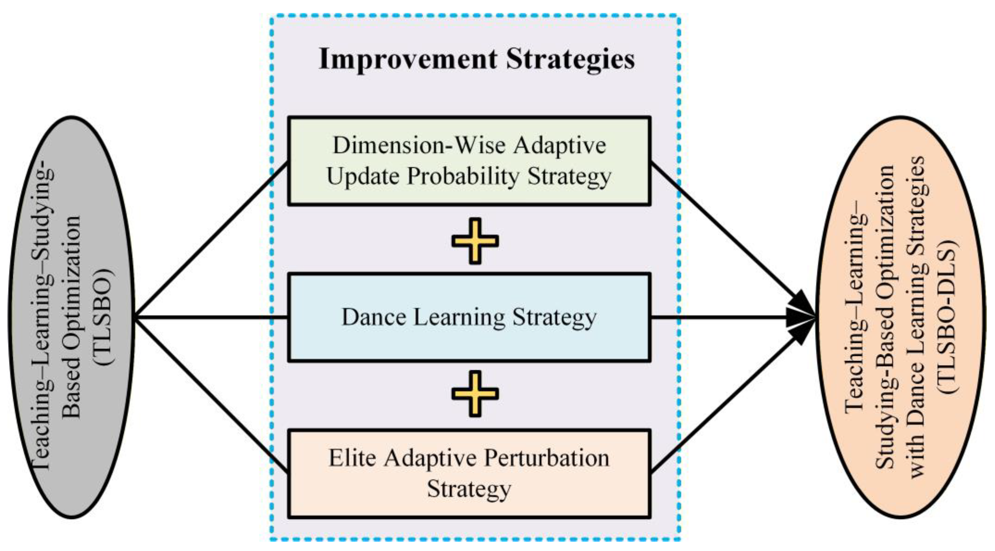
To overcome the inherent limitations of traditional TLSBO and improve WSN deployment optimization performance, this paper proposes an enhanced algorithm named TLSBO-DLS, which integrates a dance learning strategy. First, a dimension-wise adaptive update probability strategy is introduced to control the number of updated dimensions, enabling a smooth transition from global coarse search in early stages to local fine search in later stages. Second, a dance learning strategy is designed, guided by the teacher, global best, and randomly selected individuals, and incorporating sine–cosine oscillations to achieve multidirectional dynamic cooperative search, thereby enhancing exploration capability in complex regions. Third, an elite adaptive perturbation strategy based on a Cauchy–Gaussian hybrid distribution is proposed to apply adaptive perturbations to the global best solution, balancing large-step exploration in early stages with fine exploitation in later stages. Additionally, a multi-objective WSN node deployment model is constructed, and TLSBO-DLS is applied to this practical problem. The effectiveness of the proposed algorithm is validated through both benchmark functions and real-world engineering scenarios.

The main contributions of this paper are summarized as follows:

(1)

An improved algorithm, TLSBO-DLS, is proposed by integrating dimension-wise adaptive updating, dance learning, and elite adaptive perturbation strategies, significantly enhancing optimization accuracy, convergence speed, and robustness in high-dimensional complex problems.

(2)

Extensive experiments are conducted on the CEC2017, CEC2020, and CEC2022 benchmark suites, and statistical superiority is verified using the Wilcoxon rank-sum test and Friedman ranking test.

(3)

The proposed algorithm is applied to a self-constructed two-dimensional WSN node deployment problem, achieving coordinated optimization of coverage, redundancy, and movement cost, thereby providing an efficient solution for practical engineering applications.

The rest of this manuscript is structured as follows. Section 2 presents the fundamental concepts of TLSBO along with the formulation of the TLSBO-DLS approach. Section 3 provides a comparative analysis of algorithm performance using the CEC benchmark test functions. Section 4 applies the algorithm to the WSN deployment problem and validates its engineering effectiveness. Finally, Section 5 employs two classical engineering optimization problems to further validate the effectiveness of the proposed method. Section 6 concludes the paper and outlines future research directions.

2. Teaching–Learning–Studying-Based Optimization and Proposed Methodology

2.1. Teaching–Learning–Studying-Based Optimization

Teaching–Learning-Based Optimization (TLBO) [25] is a population-based metaheuristic inspired by the knowledge transfer process in a classroom environment. In this framework, each candidate solution is regarded as a learner, and the best-performing individual in the population acts as the teacher. Compared with many other algorithms, TLBO has fewer control parameters and exhibits strong performance in various optimization problems. The schematic diagram of the Teaching–Learning–Studying-Based Optimization (TLSBO) algorithm is shown in Figure 1, which consists of three main phases: the teacher phase, the learner phase, and the studying phase, corresponding to knowledge transfer, peer interaction, and individual refinement, respectively.

In TLBO, the population is denoted as ${\mathbf{X}}_i=(X_{i1},X_{i2},\dots ,X_{iD})$, where $i=\mathrm{1,2},\dots ,N$. The current best solution is denoted as $\mathbf{G}$, and the population mean is expressed as $\mathbf{M}\mathbf{e}\mathbf{a}\mathbf{n}$.

(1) Teacher Phase

The teacher phase simulates the process of knowledge dissemination from the teacher to learners. The teacher, corresponding to the best individual $\mathbf{G}$, attempts to shift the population mean toward a better level.

The position update in this phase can be expressed as:

$$X_{i,j}^{t+1}=X_{i,j}^t+r\cdot (G_j^t-T_F\cdot Mea{n}_j^t)$$

(1)

where $r\in \left(\mathrm{0,1}\right)$ is a random number, and $T_F$ is the teaching factor, typically taking values 1 or 2.

This mechanism encourages the population to move toward the teacher while adjusting the overall distribution of solutions.

(2) Learner Phase

In addition to learning from the teacher, individuals can also improve their knowledge through interaction with peers. During this phase, each learner ${\mathbf{X}}_i$ randomly selects another individual ${\mathbf{X}}_k$ for mutual learning.

The update strategy can be formulated as:

$$X_{i,j}^{t+1}=\left\{\begin{array}{c}{X}_{i,j}^t+r\cdot (X_{k,j}^t-X_{i,j}^t),\hspace{0.25em}\hspace{0.25em}\hspace{0.25em}\hspace{0.25em}f\left({\mathbf{X}}_k\right)<f\left({\mathbf{X}}_i\right)\\ X_{i,j}^t+r\cdot (X_{i,j}^t-X_{k,j}^t),\hspace{0.25em}\hspace{0.25em}\hspace{0.25em}\hspace{0.25em}\mathrm{otherwise}\hspace{0.25em}\hspace{0.25em}\hspace{0.25em}\hspace{0.25em}\hfill \end{array}\right.$$

(2)

where $r\in \left(\mathrm{0,1}\right)$, and $f(·)$ represents the objective function.

This phase enhances diversity and enables individuals to explore new regions of the search space through pairwise interaction.

2.2. Proposed Methodology (Teaching–Learning–Studying-Based Optimization with Dance Learning Strategies)

Although TLSBO achieves knowledge transfer through the Teacher and Learner phases, it still faces limitations in high-dimensional and complex optimization problems. Specifically, simultaneous multi-dimensional updates may lead to coarse search steps and reduced exploitation accuracy; population convergence reduces diversity, increasing the risk of local optima; and the simple learning mechanism lacks dynamic search flexibility.

To address these issues, three strategies are proposed while retaining the original framework. First, a dimension-wise adaptive update probability enhances fine-grained exploitation by controlling effective dimensions. Second, a Dance Learning Strategy (DLS) introduces oscillatory collaborative learning to improve exploration and escape local optima. Third, an elite adaptive perturbation based on a decaying Cauchy–Gaussian hybrid improves convergence while avoiding stagnation. Together, these strategies enhance exploration, exploitation, and convergence stability.

2.2.1. Dimension-Wise Adaptive Update Probability Strategy

In the original TLSBO, whether in the Teacher Phase or the Learner Phase, the position vector of an individual usually changes as a whole according to the updating formula; that is, all dimensions in the position vector participate in the update simultaneously. Let the position vector of the $i$-th individual at the $t$-th iteration be

$${\mathbf{X}}_i^t=[x_{i,1}^t,x_{i,2}^t,\dots ,x_{i,D}^t]\in {\mathbb{R}}^{1\times D},$$

(3)

where $D$ denotes the problem dimension and is a positive integer scalar; ${\mathbf{X}}_i^t$ is a row vector of size $1\times D$; and $x_{i,d}^t$ denotes the position of the $i$-th individual in the $d$-th dimension and is a scalar. If all dimensions change simultaneously in each update, two phenomena are likely to occur in high-dimensional complex problems. On the one hand, the search in the early stage becomes too aggressive, leading to increased directional fluctuation. On the other hand, synchronous perturbation of multiple dimensions in the later stage may destroy the local structure that is already close to the optimum, thereby reducing the fine search capability.

To this end, a dimension-wise adaptive update probability strategy is introduced in this paper. Its core idea is that, after a candidate solution is obtained according to the original TLSBO updating formula, not all dimensions are allowed to immediately adopt the new values. Instead, only part of the dimensions are allowed to be updated according to a certain probability, while the remaining dimensions keep their original values unchanged. In this way, the algorithm can maintain full-dimensional search with high freedom in the early stage, and gradually transition to local fine exploitation dominated by partial dimensions in the later stage.

Let ${\mathbf{Y}}_i^t\in {\mathbb{R}}^{1\times D}$ denote the candidate position vector generated by the original Teacher Phase or Learner Phase updating formula, and let its $d$-th component is denoted by $y_{i,d}^t.$ Define the dimension update probability at iteration $t$ as

$$P_c^t=P_c^{max}-\left(P_c^{max}-P_c^{min}\right){\displaystyle \frac{t}{T_{max}}},$$

(4)

where $P_c^t$ is a scalar representing the probability that a single dimension is updated at the current iteration; $P_c^{max}$ and $P_c^{min}$ are the initial and terminal values of the dimension update probability, respectively, and satisfy $0<P_c^{min}<P_c^{max}\le 1$; $t$ is the current iteration number and is a positive integer scalar; and $T_{max}$ is the maximum number of iterations and is also a positive integer scalar.

It can be seen from (4) that, as the iteration proceeds, $P_c^t$ decreases monotonically. That is, more dimensions participate in updating in the early stage, while fewer dimensions participate in updating in the later stage, thus realizing a smooth transition from coarse-grained global search to fine-grained local exploitation.

Furthermore, define the dimension mask vector as

$${\mathbf{M}}_i^t=[m_{i,1}^t,m_{i,2}^t,\dots ,m_{i,D}^t]\in \{\mathrm{0,1}{\}}^{1\times D},$$

(5)

where $m_{i,d}^t$ is a Bernoulli random variable satisfying:

$$m_{i,d}^t=\left\{\begin{array}{c}1,\hspace{0.25em}\hspace{0.25em}\hspace{0.25em}\hspace{0.25em}\mathrm{if} rand<P_c^t,\hfill \\ 0,\hspace{0.25em}\hspace{0.25em}\hspace{0.25em}\hspace{0.25em}\mathrm{o}\mathrm{t}\mathrm{h}\mathrm{e}\mathrm{r}\mathrm{w}\mathrm{i}\mathrm{s}\mathrm{e},\hspace{0.25em}\hspace{0.25em}\hspace{0.25em}\hspace{0.25em}\end{array}\right.$$

(6)

where $rand$ is a random scalar uniformly distributed over the interval [0, 1]. To avoid the case where no dimension is selected in an iteration and the individual is therefore not updated at all, when ${\displaystyle {\sum }_{d=1}^D} m_{i,d}^t=0,$ a dimension $d^{\ast }\in \{\mathrm{1,2},\dots ,D\}$ is randomly selected, and $m_{i,d^{\ast }}^t=1$ is enforced.

Accordingly, the final updated position vector of the iii-th individual can be written as

$${\mathbf{X}}_{i,\mathrm{n}\mathrm{e}\mathrm{w}}^t={\mathbf{X}}_i^t+{\mathbf{M}}_i^t\odot \left({\mathbf{Y}}_i^t-{\mathbf{X}}_i^t\right),$$

(7)

where $\odot$ denotes the Hadamard element-wise multiplication; and ${\mathbf{X}}_{i,\mathrm{n}\mathrm{e}\mathrm{w}}^t$ is the final updated position vector.

The essence of this strategy lies in that the algorithm no longer forces all dimensions to be updated simultaneously, but screens the dimensions participating in the update through an adaptive probability. Since $P_c^t$ is large in the early stage, more dimensions participate in updating, and the population still maintains strong global exploration capability. In contrast, $P_c^t$ becomes smaller in the later stage, and only a small number of important dimensions are adjusted, thereby weakening ineffective perturbations and improving local exploitation accuracy. Therefore, this strategy can improve the convergence stability and optimization accuracy of the algorithm in high-dimensional complex problems without changing the basic structure of TLSBO.

2.2.2. Dance Learning Strategy

Although the dimension-wise adaptive update probability strategy can improve the granularity of individual updates, the basic learning behavior of TLSBO is still mainly reflected as a direct displacement of “learning from the teacher” or “learning from peers,” and its search pattern remains relatively simple. When the population gradually gathers in some promising regions during the middle and later stages, the movement directions of individuals tend to become consistent, which in turn causes the search trajectory to become rigid and reduces the exploration ability in complex local regions. To enhance the dynamic cooperative search ability of the population near promising regions, a Dance Learning Strategy is proposed in this paper.

The basic idea of the Dance Learning Strategy is as follows: after the conventional Teacher Phase and Learner Phase are completed, each individual performs collaborative learning with periodic oscillatory characteristics around the teacher individual, the current global best individual, and a randomly selected peer differential direction. Different from the traditional one-way approach, this strategy constructs multidirectional dynamic oscillatory updates through sine and cosine oscillation terms, so that individuals can perform more flexible “back-and-forth probing” near promising regions, thereby enhancing the ability to identify complex local structures and improving the possibility of escaping from local optima.

Let the position vector of the teacher individual at iteration $t$ be ${\mathbf{T}}^t=[T_1^t,T_2^t,\dots ,T_D^t]\in {\mathbb{R}}^{1\times D}$, and let the position vector of the current global best individual be ${\mathbf{G}}^t=[G_1^t,G_2^t,\dots ,G_D^t]\in {\mathbb{R}}^{1\times D}$.

Randomly select two individuals from the population that are different from the $i$-th individual, and denote their position vectors by ${\mathbf{x}}_{r_1}^t,{\mathbf{x}}_{r_2}^t\in {\mathbb{R}}^{1\times D}$($r_1\ne r_2\ne i$). Define the candidate position vector generated by dance learning as

$${\mathbf{Z}}_i^t={\mathbf{X}}_i^t+{\beta }^t\mathrm{s}\mathrm{i}\mathrm{n}\left(2\pi {\mathbf{R}}_1^t\right)\odot ({\mathbf{T}}^t-{\mathbf{X}}_i^t)+{\gamma }^t\mathrm{c}\mathrm{o}\mathrm{s}\left(2\pi {\mathbf{R}}_2^t\right)\odot ({\mathbf{G}}^t-{\mathbf{X}}_i^t)+{\eta }^t{\mathbf{R}}_3^t\odot ({\mathbf{X}}_{r_1}^t-{\mathbf{X}}_{r_2}^t),$$

(8)

where ${\mathbf{Z}}_i^t$ is the candidate position vector generated by dance learning; ${\mathbf{R}}_1^t,{\mathbf{R}}_2^t,{\mathbf{R}}_3^t$ are random vectors following uniform distributions, and each component is an independent random scalar; $\mathrm{s}\mathrm{i}\mathrm{n}\left(2\pi {\mathbf{R}}_1^t\right)$ and $\mathrm{c}\mathrm{o}\mathrm{s}\left(2\pi {\mathbf{R}}_2^t\right)$ denote the element-wise sine and cosine operations on the vectors, respectively; and ${\beta }^t,{\gamma }^t, \mathrm{a}\mathrm{n}\mathrm{d} {\eta }^t$ are all nonnegative scalars, which control the influence intensities of the “oscillation toward the teacher,” “oscillation toward the global best,” and the “population differential rhythmic term,” respectively.

To make this strategy emphasize dynamic exploration in the early stage and stable convergence in the later stage, the following adaptive decay coefficients are introduced:

$${\displaystyle \genfrac{}{}{0pt}{}{{\beta }^t={\beta }_0\left(1-\frac{t}{T_{max}}\right),}{\begin{array}{c}{\gamma }^t={\gamma }_0\left(1-\frac{t}{T_{max}}\right),\\ {\eta }^t={\eta }_0\left(1-\frac{t}{T_{max}}\right),\end{array}}}$$

(9)

where ${\beta }_0$, ${\gamma }_0$, and ${\eta }_0$ are predefined positive scalar constants, representing the maximum initial strengths of the three dance-learning components, respectively. Since the coefficients in (19) all decrease linearly with the iteration, individuals can oscillate around promising regions with relatively large amplitudes in the early stage, whereas the oscillation amplitude gradually shrinks in the later stage, thereby avoiding damage to the high-quality solutions already obtained.

In addition, to prevent dance learning from being triggered too frequently throughout the entire optimization process and thus affecting the later convergence, its triggering probability is further defined as

$$P_d^t=P_d^{max}-\left(P_d^{max}-P_d^{min}\right){\displaystyle \frac{t}{T_{max}}},$$

(10)

where $P_d^t$ is the triggering probability of the dance learning strategy at iteration $t$, and is a scalar; $P_d^{max}$ and $P_d^{min}$ are the initial and terminal triggering probabilities, respectively, satisfying $0<P_d^{min}<P_d^{max}<1$. When $rand<P_d^t$, the $i$-th individual executes the dance learning update; otherwise, the conventional updated result remains unchanged.

Considering that the dimension-wise adaptive update probability has already been introduced in the previous strategy, the candidate solution generated by dance learning can also be screened through the dimension mask. Its final form can be expressed as

$${\mathbf{X}}_{i,\mathrm{d}\mathrm{a}\mathrm{n}\mathrm{c}\mathrm{e}}^t={\mathbf{X}}_i^t+{\mathbf{M}}_i^t\odot ({\mathbf{Z}}_i^t-{\mathbf{X}}_i^t),$$

(11)

The essence of this strategy lies in the fact that individuals no longer directly approach only the teacher or the global best along a single direction, but perform a multidirectional search near promising regions in a periodic oscillatory manner under the joint guidance of multiple advantageous sources of information. Specifically, the first term uses the teacher individual to provide the dominant learning direction; the second term uses the current global best individual to strengthen the focus on high-quality regions; and the third term uses a random peer differential vector to maintain population dynamics and directional diversity. The combined action of these three components can effectively enhance the dynamic search capability of the algorithm in complex multimodal regions and alleviate the problem of premature rigidity of the search trajectory.

2.2.3. Elite Adaptive Perturbation Strategy

Although the above two strategies can improve the search behavior of TLSBO, respectively, from the perspectives of dimension update granularity and population dynamic learning mode, when the population has already converged to a certain locally promising region in the middle and later stages, the current global best individual may still remain unchanged for a long time. If one relies only on the updates of ordinary individuals to further improve the best solution, it is often difficult to break local stagnation in time. Therefore, this paper further proposes an elite adaptive perturbation strategy, which directly performs local refinement and jump-based probing on the current global best individual.

The core idea of this strategy is as follows: at the end of each iteration, an adaptively decaying Cauchy–Gaussian hybrid perturbation is imposed on the current global best position vector ${\mathbf{G}}^t$. Since the Cauchy distribution has a heavy-tailed property, it is more likely to generate large jumps and is therefore suitable for helping the best solution escape from local optima in the early stage or during stagnation. In contrast, the perturbation generated by the Gaussian distribution is relatively smooth and is more suitable for local fine search in the later stage. Therefore, adaptively combining the two can simultaneously take into account both jumping ability and refinement ability.

Define the Cauchy random vector and the Gaussian random vector as

$${\displaystyle \genfrac{}{}{0pt}{}{{\mathbf{C}}^t=[C_1^t,C_2^t,\dots ,C_D^t]\in {\mathbb{R}}^{1\times D},}{{\mathbf{N}}^t=[N_1^t,N_2^t,\dots ,N_D^t]\in {\mathbb{R}}^{1\times D},}}$$

(12)

where $C_d^t$ follows the standard Cauchy distribution, and  $N_d^t$ follows the standard normal distribution. The components of both vectors are random scalars.

Define the adaptive mixing coefficient as

$${\alpha }^t=1-{\displaystyle \frac{t}{T_{max}}},$$

(13)

where ${\alpha }^t\in \left[\mathrm{0,1}\right]$ is a scalar. It can be seen from (13) that in the early stage of the iteration, ${\alpha }^t$ is relatively large, and the Cauchy component dominates; whereas in the later stage, ${\alpha }^t$ becomes smaller, and the Gaussian component gradually dominates.

Further define the perturbation scale vector as

$${\mathit{\delta }}^t=\lambda \left(1-{\displaystyle \frac{t}{T_{max}}}\right)(\mathbf{U}-\mathbf{L}),$$

(14)

where $\mathbf{U}$ and $\mathbf{L}$ are the upper-bound vector and lower-bound vector of the search space, respectively. $\lambda$ is a constant scalar used to control the perturbation intensity. Equation (14) shows that the perturbation scale gradually decreases as the iteration proceeds, so that the perturbation range is larger in the early stage and finer in the later stage.

Accordingly, the candidate position vector generated by elite perturbation is defined as

$${\mathbf{G}}_{\mathrm{e}\mathrm{l}\mathrm{i}\mathrm{t}\mathrm{e}}^t={\mathbf{G}}^t+{\delta }^t\odot \left({\alpha }^t{\mathbf{C}}^t+\left(1-{\alpha }^t\right){\mathbf{N}}^t\right).$$

(15)

where ${\mathbf{G}}_{\mathrm{e}\mathrm{l}\mathrm{i}\mathrm{t}\mathrm{e}}^t$ is the elite-perturbation candidate solution. This equation indicates that the perturbation of the best individual in each dimension is jointly determined by three factors. First, the boundary scale $\left(\mathbf{U}-\mathbf{L}\right)$ ensures that the perturbation of each dimension matches the search range of that dimension. Second, ${\alpha }^t$ controls the relative proportion of the Cauchy and Gaussian perturbations. Third, the overall coefficient $\lambda \left(1-{\displaystyle \frac{t}{T_{max}}}\right)$ causes the perturbation magnitude to decay with the iteration.

After ${\mathbf{G}}_{\mathrm{e}\mathrm{l}\mathrm{i}\mathrm{t}\mathrm{e}}^t$ is obtained, boundary constraint handling is required. Let the vector after boundary handling be

$${\tilde{\mathbf{G}}}_{\mathrm{e}\mathrm{l}\mathrm{i}\mathrm{t}\mathrm{e}}^t=min\left(max({\mathbf{G}}_{\mathrm{e}\mathrm{l}\mathrm{i}\mathrm{t}\mathrm{e}}^t,\mathbf{L}),\mathbf{U}\right),$$

(16)

Subsequently, the fitness of ${\tilde{\mathbf{G}}}_{\mathrm{e}\mathrm{l}\mathrm{i}\mathrm{t}\mathrm{e}}^t$ is evaluated. If its fitness is better than that of the current global best individual, it replaces ${\mathbf{G}}^t$. At the same time, in order to strengthen the feedback effect of elite information on the population, the updated global best individual can further be used to replace the worst individual in the current population. Let the objective function be $f(·)$. Then, the elite updating criterion can be written as

$$\mathrm{i}\mathrm{f} f({\tilde{\mathbf{G}}}_{\mathrm{e}\mathrm{l}\mathrm{i}\mathrm{t}\mathrm{e}}^t)<f({\mathbf{G}}^t),{\mathbf{G}}^t\leftarrow {\tilde{\mathbf{G}}}_{\mathrm{e}\mathrm{l}\mathrm{i}\mathrm{t}\mathrm{e}}^t.$$

(17)

The advantage of this strategy lies in that it does not add extra random perturbations to all individuals, but only performs controlled adaptive correction on the current best individual. Therefore, it does not significantly destroy the overall convergence trend of the population. Meanwhile, because the Cauchy component is strong in the early stage, the best individual gains a certain large-step jumping ability, which can help the algorithm escape from local optima. In the later stage, the Gaussian component dominates and the perturbation becomes smoother, which is beneficial for fine exploitation near the optimum region. Therefore, the elite adaptive perturbation strategy can effectively enhance the local deep search ability and stagnation escape ability of TLSBO in the middle and later stages.

After embedding the above three strategies into TLSBO, the improved algorithm significantly strengthens its internal search dynamics while preserving the original dual-phase main framework of the Teacher Phase and Learner Phase. Specifically, the dimension-wise adaptive update probability strategy controls the number of dimensions that truly change in each update, enabling the algorithm to maintain a high degree of global exploration freedom in the early stage and reduce ineffective perturbations in the later stage, thereby enhancing local exploitation accuracy. The Dance Learning Strategy provides individuals, in addition to conventional learning behavior, with a multidirectional periodic oscillatory search mode around the teacher individual, the global best individual, and peer differential vectors, thereby improving the cooperative search ability and dynamic jumping ability of the population in complex regions. The elite adaptive perturbation strategy directly acts on the current global best individual, and realizes a smooth transition from large-step jumping to fine-grained refinement through Cauchy–Gaussian hybrid perturbations at different stages, further enhancing the ability of the algorithm to escape from local stagnation.

The integration of the three proposed strategies enhances TLSBO from complementary perspectives. The dimension-adaptive update mechanism improves fine-grained search control, the dance learning strategy increases population diversity and exploration flexibility, and the elite perturbation mechanism strengthens local exploitation and stagnation escape ability. Their combination leads to a balanced exploration–exploitation trade-off and significantly improves overall optimization performance.

Based on the above description, the pseudocode of TLSBO-DLS is presented in Algorithm 1 and the overall framework of TLSBO-DLS is shown in Figure 2.

Algorithm 1. Pseudocode of TLSBO-DLS.

Input$: \mathrm{population} \mathrm{size} N$$, \mathrm{maximum} \mathrm{iteration} T_{max}$$, \mathrm{dimension} D$$, \mathrm{lower} \mathrm{bound} \mathbf{L}$$, \mathrm{upper} \mathrm{bound} \mathbf{U}$. Output$: \mathrm{Best} \mathrm{solution} \mathbf{G}$$, \mathrm{and} \mathrm{best} \mathrm{fitness} f\left(\mathbf{G}\right).$ 1: Randomly initialize the population ${\mathbf{X}}_i\left(i=\mathrm{1,2},\dots ,N\right)$ within the search range. $2:\mathrm{Compute} \mathrm{the} \mathrm{objective} \mathrm{values} \mathrm{for} \mathrm{every} \mathrm{candidate} \mathrm{and} \mathrm{identify} \mathrm{the} \mathrm{presently} \mathrm{optimal} \mathrm{global} \mathrm{solution} \mathbf{G}.$ 3: while $t=1:T_{max}$ then $4: \mathrm{Compute} \mathrm{the} \mathrm{mean} \mathrm{position} \mathbf{M}\mathbf{e}\mathbf{a}\mathbf{n}$$\mathrm{and} \mathrm{Select} \mathrm{the} \mathrm{teacher} \mathrm{individual} \mathbf{T}$ according to the current best fitness. $5: \mathrm{Compute} \mathrm{the} \mathrm{dimension}\text{-}\mathrm{wise} \mathrm{adaptive} \mathrm{update} \mathrm{probability} P_c^t$ according to Equation (4). $6: \mathrm{Compute} \mathrm{the} \mathrm{dance} \mathrm{learning} \mathrm{activation} \mathrm{probability} P_d^t$ according to Equation (10). $7: \mathit{for} \mathrm{for} \mathrm{each} \mathrm{individual} i$ do $8: \mathrm{Generate} \mathrm{the} \mathrm{teacher}\text{-}\mathrm{phase} \mathrm{candidate} \mathrm{solution} {\mathbf{Y}}_i^t$ according to the original TLSBO teacher updating rule. $9: \mathrm{Generate} \mathrm{the} \mathrm{dimension} \mathrm{mask} \mathrm{vector} {\mathbf{M}}_i^t$ according to Equations (5) and (6). $10: \mathrm{Construct} \mathrm{the} \mathrm{teacher}\text{-}\mathrm{phase} \mathrm{updated} \mathrm{solution} {\mathbf{X}}_{i,\mathrm{n}\mathrm{e}\mathrm{w}}^t$ according to Equation (7). $11: \mathit{if} rand<P_d^t$ then $12: \mathrm{Generate} \mathrm{the} \mathrm{dance} \mathrm{learning} \mathrm{candidate} \mathrm{solution} {\mathbf{Z}}_i^t$ according to Equation (8). $13: \mathrm{Construct} \mathrm{the} \mathrm{dance} \mathrm{learning} \mathrm{updated} \mathrm{solution} {\mathbf{X}}_{i,\mathrm{d}\mathrm{a}\mathrm{n}\mathrm{c}\mathrm{e}}^t$ according to Equation (11). 14:       end if $15: \mathrm{Evaluate} \mathrm{the} \mathrm{fitness} \mathrm{of} {\mathbf{X}}_{i,\mathrm{n}\mathrm{e}\mathrm{w}}^t$$\mathrm{and} {\mathbf{X}}_{i,\mathrm{d}\mathrm{a}\mathrm{n}\mathrm{c}\mathrm{e}}^t$ 16:    Update the current individual if the new solution is better. $17: \mathrm{Update} \mathrm{the} \mathrm{global} \mathrm{best} \mathrm{solution} \mathbf{G}$ if a better individual is found. 18:     end for $19: \mathrm{Compute} \mathrm{the} \mathrm{adaptive} \mathrm{mixing} \mathrm{coefficient} {\alpha }^t$ according to Equation (13). $20: \mathrm{Compute} \mathrm{the} \mathrm{perturbation} \mathrm{scale} \mathrm{vector} {\mathit{\delta }}^t$ according to Equation (14). $21: \mathrm{Generate} \mathrm{the} \mathrm{elite} \mathrm{perturbation} \mathrm{candidate} \mathrm{solution} {\mathbf{G}}_{\mathrm{e}\mathrm{l}\mathrm{i}\mathrm{t}\mathrm{e}}^t$ according to Equation (15). $22: \mathrm{Perform} \mathrm{boundary} \mathrm{control} \mathrm{on} {\mathbf{G}}_{\mathrm{e}\mathrm{l}\mathrm{i}\mathrm{t}\mathrm{e}}^t$ according to Equation (16). $23: \mathit{if} f\left({\mathbf{G}}_{\mathrm{e}\mathrm{l}\mathrm{i}\mathrm{t}\mathrm{e}}^t\right)<f\left(\mathbf{G}\right)$ then 24:        Update the global best solution according to Equation (17). 25:        Replace the worst individual in the population with the updated global best solution. 26:    end if $27: t=t+1.$ 28: end while 29: $\mathrm{Return} \mathbf{G}$$\mathrm{and} f\left(\mathbf{G}\right)$.

The algorithm proceeds sequentially as follows: first, the teacher phase is executed with dimension-adaptive updates. Then, with a certain probability, the dance learning strategy is applied to enhance exploration. After evaluating individuals, the learner phase is implicitly included through pairwise interactions. Finally, the elite perturbation mechanism is applied to refine the global best solution.

2.3. Computational Complexity Analysis

To evaluate the computational efficiency of the proposed TLSBO-DLS algorithm, a detailed complexity analysis is conducted in comparison with the original TLSBO framework. Let $N$ denote the population size, $D$ the problem dimensionality, and $T$ the maximum number of iterations. In the original TLSBO, each iteration consists of the teacher phase, learner phase, and studying phase, where all individuals are updated across all dimensions. Since each individual update involves vector operations of dimension $D$, the computational cost per individual is $O\left(D\right)$, leading to a total complexity of $O(N \times D)$ per iteration. Consequently, over T iterations, the overall computational complexity of TLSBO is $O(T \times N \times D)$.

In the proposed TLSBO-DLS algorithm, three additional strategies are incorporated into the original framework. The dimension-wise adaptive update mechanism introduces a masking operation that selectively updates certain dimensions, which requires generating D random variables and performing element-wise operations for each individual. This results in an additional computational cost of $O\left(D\right)$ per individual, and thus $O(TN \times D)$ per iteration. The dance learning strategy further enhances the search process by introducing oscillatory updates based on sine and cosine functions. Although this strategy is triggered with a certain probability, its expected computational cost remains proportional to $O(N \times D)$, as each activated update still involves vector operations across all dimensions. Furthermore, the elite adaptive perturbation strategy operates only on the current global best individual, requiring the generation of Cauchy and Gaussian random vectors and corresponding vector operations, which introduces an additional cost of $O\left(D\right)$ per iteration.

By combining all components, the total computational complexity of TLSBO-DLS per iteration can be expressed as $O(N \times D)$, since the additional strategies do not change the dominant term but only introduce a moderate increase in the constant factor. Therefore, the overall complexity over T iterations remains $O(T \times N \times D)$ which is consistent with that of the original TLSBO algorithm. From a practical perspective, although the proposed strategies introduce extra operations such as random sampling and trigonometric calculations, their computational overhead is relatively small compared to the overall population update process. As a result, TLSBO-DLS achieves a significant improvement in optimization performance while maintaining a comparable computational cost, making it suitable for solving high-dimensional and complex optimization problems efficiently.

3. IEEE CEC Standard Test Suite Evaluation

3.1. Algorithms for Comparison and Parameter Configuration

To assess the effectiveness of the proposed method, a series of experiments is conducted using benchmark functions from the CEC2017, CEC2020, and CEC2022 suites, aiming to evaluate the optimization performance of TLSBO-DLS. The results are compared with several classical optimization techniques, including Particle Swarm Optimization (PSO) [9], Grey Wolf Optimizer (GWO) [10], and Whale Optimization Algorithm (WOA) [33]. In addition, comparisons are made with more recent algorithms, including the Artificial Lemming Algorithm (ALA) [34], and Secretary Bird Optimization Algorithm(SBOA) [17]. Furthermore, the proposed method is evaluated against different variants of TLSBO, namely Teaching–Learning–Studying-Based Optimization (TLSBO) [25], the Teaching–Learning Optimization Algorithm incorporating Cadre–Mass relationships with a tutor mechanism (TLOCTO) [35], an Improved Teaching-Learning-Based Optimization Algorithm with Reinforcement Learning Strategy (RLTLBO) [36], and an improved version integrating Cauchy mutation and chaotic operators (PI-CTLBO) [37]. Detailed parameter settings for all compared methods are summarized in

Table 1. Summary of the parameter configurations used for all comparative algorithms.

Algorithm	Parameter	Value
PSO	$c_1,c_2, w$	2, 2, 0.8
GWO	$a$	[0, 2]
WOA	$r,l,a$	[0, 1], [−1, 1], Linear reduction from 2 to 1
ALA	$Prob$	$0.3$
SBOA	$CF,K, RB$	$\left[0, 1\right],\left\{1, 2\right\},[0,1]$
TLSBO	$TF$	$\left\{1, 2\right\}$
TLOCTO	$TF,\kappa$	$\left\{1, 2\right\}, 1.5$
RLTLBO	$TF,\alpha ,\gamma$	$\left\{1, 2\right\},0.1, 0.8$
PI-CTLBO	$TF$	$\left\{1, 2\right\}$

.

The parameter settings of all comparative algorithms are selected according to their original literature or widely adopted configurations in recent studies to ensure fairness and reproducibility. For the proposed TLSBO-DLS, the parameter values were determined based on preliminary experiments, balancing convergence speed and solution accuracy.

To guarantee an unbiased comparison and minimize stochastic effects, a consistent experimental setup was employed. In detail, each method operated with a swarm size of 30, while the termination condition was defined as 1000 generations. Every algorithm was executed 30 independent times to obtain reliable performance data. The evaluation metrics included the mean performance (Mean) and the dispersion measure (Std), and the optimal results were emphasized in boldface for clarity. All numerical experiments were implemented on a workstation running Windows 11, powered by an Intel^® Core™ i5-series processor (13th Gen, Intel Corporation, Santa Clara, CA, USA) with a base clock speed around 2.5 GHz and 16 GB memory, and MATLAB R2022b was used as the simulation environment.

3.2. Ablation Study

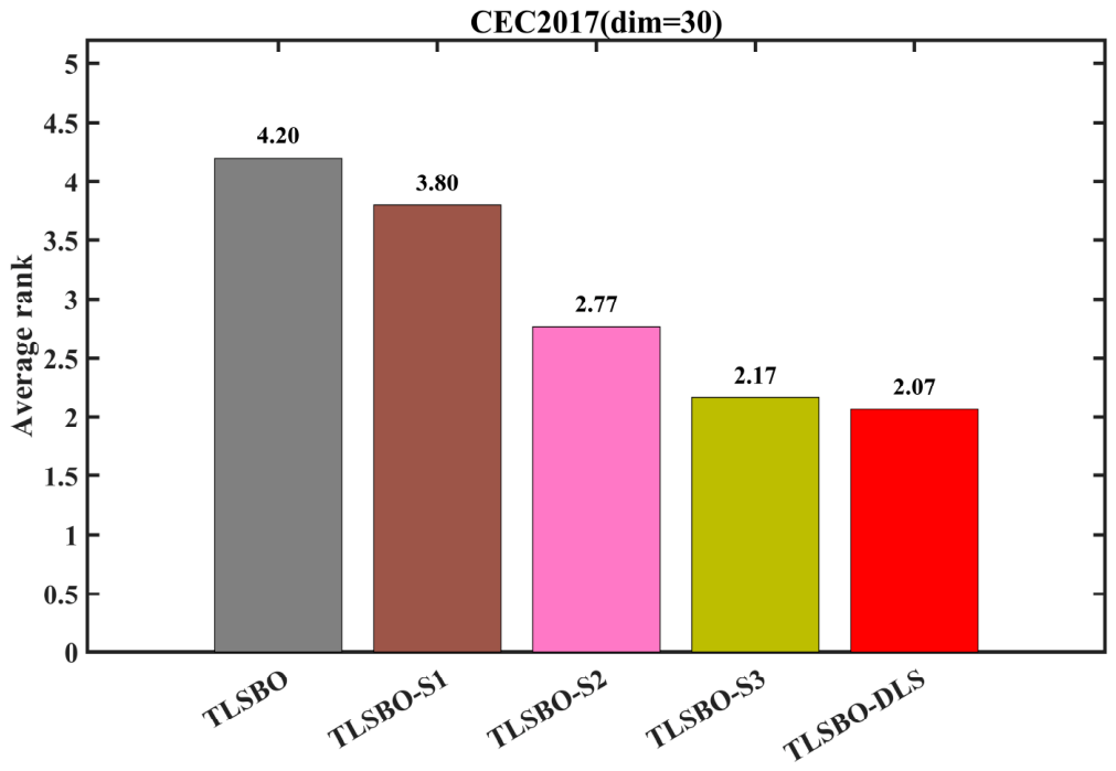
To clearly quantify the individual contributions and synergistic effects of the three proposed improvement strategies, an ablation study was designed based on the CEC2017 benchmark suite (30 dimensions). Three improved variants incorporating a single strategy were constructed, namely TLSBO-S1 (dimension-adaptive update probability strategy), TLSBO-S2 (dance learning strategy), and TLSBO-S3 (elite adaptive perturbation strategy). These variants were compared with the original TLSBO and the final integrated algorithm TLSBO-DLS. The mean rank was utilized as the assessment criterion, with lower values reflecting superior comprehensive performance. The corresponding outcomes are illustrated in Figure 3.

As illustrated in Figure 3, the average ranking values of the five algorithms are as follows: the original TLSBO achieves 4.20, TLSBO-S1 obtains 3.80, TLSBO-S2 reaches 2.77, TLSBO-S3 achieves 2.17, and TLSBO-DLS, which integrates all three strategies, attains the best value of 2.07. Accordingly, the performance ranking from worst to best is: TLSBO < TLSBO-S1 < TLSBO-S2 < TLSBO-S3 < TLSBO-DLS.

First, compared with the original TLSBO, all variants incorporating a single strategy exhibit clear performance improvements. Specifically, TLSBO-S1 reduces the average ranking value to 3.80, representing an improvement of 0.40, indicating that the dimension-adaptive update strategy effectively enhances the update mechanism and improves search efficiency. TLSBO-S2 achieves a ranking value of 2.77, improving by 1.43 compared with the baseline, which is the most significant improvement among the single-strategy variants. This demonstrates that the dance learning strategy plays a crucial role in enhancing population exploration and preventing premature convergence. TLSBO-S3 further reduces the ranking value to 2.17, with an improvement of 2.03, indicating that the elite adaptive perturbation strategy effectively refines the perturbation mechanism applied to elite individuals, thereby improving local search accuracy and enhancing the ability to escape local optima.

Second, among the three single-strategy variants, TLSBO-S3 achieves the best performance (2.17), followed by TLSBO-S2 (2.77), while TLSBO-S1 performs relatively weaker (3.80). This observation reflects the differences in contribution among the three strategies and further indicates that the elite adaptive perturbation strategy and the dance learning strategy provide more substantial performance gains.

Finally, the proposed TLSBO-DLS, which integrates all three strategies, achieves the lowest average ranking value of 2.07. It not only significantly outperforms the original TLSBO (with an improvement of 2.13), but also surpasses all single-strategy variants. Compared with the best-performing single-strategy variant, TLSBO-S3, TLSBO-DLS further reduces the ranking value by 0.10. This result confirms that the three strategies do not simply produce additive effects, but instead exhibit strong synergistic interactions: the dimension-adaptive update strategy improves the granularity of the search process, the dance learning strategy enhances global exploration flexibility, and the elite adaptive perturbation strategy strengthens local exploitation accuracy. Their complementary integration jointly leads to a further improvement in overall algorithm performance.

3.3. Parameter Sensitivity Analysis

To investigate the effect of the perturbation intensity parameter λ in the elite adaptive perturbation strategy, a sensitivity analysis was conducted based on Equation (14), where $\lambda$ controls the magnitude of the perturbation scale. According to this formulation, the perturbation scale gradually decreases as the iteration proceeds, enabling large exploration steps in the early stage and refined exploitation in the later stage. 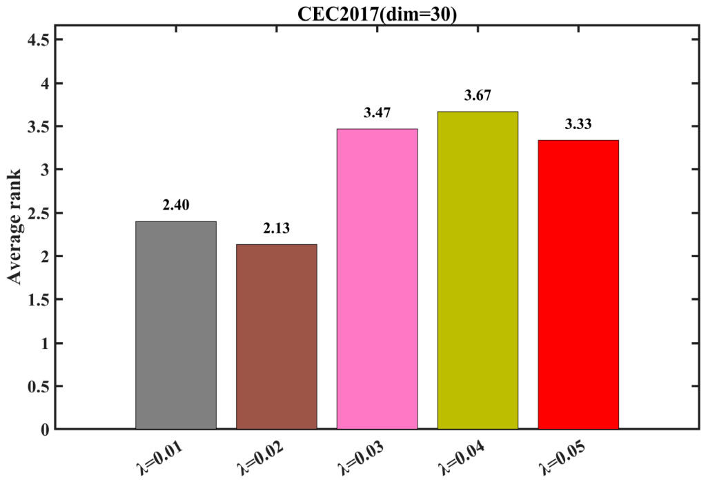In this study, $\lambda$ was set to five different values, namely 0.01, 0.02, 0.03, 0.04, and 0.05, while keeping all other parameters unchanged, in order to evaluate its impact on the optimization performance of TLSBO-DLS. The mean rank was employed as the evaluation indicator, where lower values signify superior overall effectiveness. The corresponding experimental findings are illustrated in Figure 4.

As shown in Figure 4, the average ranking values under different $\lambda$ settings are clearly reported: when $\lambda =0.01$, the algorithm achieves an average ranking value of 2.40; when $\lambda =0.02$, the ranking value decreases to 2.13; when $\lambda =0.03$, it increases to 3.47; when $\lambda =0.04$, it further rises to 3.67; and when $\lambda =0.05$, it slightly decreases to 3.33. Overall, the performance exhibits a trend of first improvement and then degradation as $\lambda$ increases. The best performance is achieved at $\lambda =0.02$, with the lowest average ranking value of 2.13 among all tested settings. When $\lambda$ exceeds 0.02, a noticeable decline in performance is observed, with the worst result occurring at $\lambda =0.04$, where the ranking value reaches 3.67.

From the perspective of the parameter mechanism, $\lambda$, as a key factor controlling the intensity of local perturbations, directly influences the balance between exploration and exploitation. When $\lambda$ is too small (e.g., 0.01), the perturbation strength is insufficient, limiting the algorithm’s ability to escape local optima, and resulting in slightly inferior performance compared to the optimal setting. When $\lambda =0.02$, the perturbation intensity is well matched with the overall search dynamics, ensuring both sufficient local exploitation accuracy and effective avoidance of local optima, thereby achieving a desirable balance between exploration and exploitation. In contrast, when $\lambda$ is too large (e.g., 0.03, 0.04, 0.05), excessive perturbations disrupt the fine-grained local search process, preventing stable convergence to high-quality solutions and leading to a significant performance degradation.

These results demonstrate that the parameter λ has a substantial impact on the performance of the TLSBO-DLS algorithm, and its optimal value lies within a specific range rather than at the extremes. Under the CEC2017 (30-dimensional) benchmark setting, $\lambda =0.02$ yields the best overall optimization performance, providing a reliable basis for parameter selection in subsequent experiments.

3.4. Experimental Analysis on the IEEE CEC Benchmark Suite

3.4.1. Experimental Analysis on the IEEE CEC2017 Benchmark Suite

To comprehensively validate the optimization performance of the proposed TLSBO-DLS algorithm on complex global optimization problems, this section conducts comparative experiments using the CEC2017 benchmark suite. This benchmark comprises various types of functions, including unimodal, multimodal, hybrid, and composite functions, which effectively evaluate the algorithm’s global exploration capability, local exploitation ability, convergence speed, and robustness [38,39,40]. It can objectively reflect the algorithm’s performance in high-dimensional and complex optimization scenarios; therefore, it is selected as the core benchmark for performance evaluation. The outcomes of the experiments are presented in

Table 2. Performance comparison of different methods on the CEC2017 test functions (30-dimensional cases).

Function	Metric	PSO	GWO	WOA	ALA	SBOA	TLSBO	TLOCTO	RLTLBO	PI-CTLBO	TLSBO-DLS
F1	Mean	2.2658E+09	2.4241E+09	1.6704E+09	3.5614E+06	3.2772E+04	3.4592E+03	2.0058E+09	1.4851E+05	2.1405E+09	3.5591E+03
	Std	2.6745E+09	1.6066E+09	6.8726E+08	1.7112E+06	1.1768E+05	4.5649E+03	3.1185E+09	6.4591E+05	1.0673E+09	3.7332E+03
F2	Mean	5.0946E+35	3.9190E+32	6.6880E+32	2.5744E+20	5.6785E+16	8.9159E+22	1.0387E+31	1.6632E+21	9.3427E+33	5.0973E+10
	Std	2.7904E+36	1.1949E+33	3.0233E+33	7.4647E+20	2.0095E+17	4.8454E+23	4.1215E+31	7.3005E+21	2.8856E+34	2.3977E+11
F3	Mean	3.2369E+04	5.0971E+04	2.5551E+05	1.1985E+04	2.4536E+04	3.3349E+04	3.4000E+03	7.3159E+03	6.4089E+03	4.2236E+04
	Std	1.0237E+04	1.1372E+04	5.9776E+04	4.3948E+03	6.2268E+03	1.6629E+04	2.4194E+03	3.1476E+03	4.7636E+03	1.1884E+04
F4	Mean	5.8811E+02	6.4463E+02	8.9231E+02	5.1197E+02	5.0880E+02	4.9078E+02	9.2781E+02	5.0429E+02	9.5765E+02	4.8528E+02
	Std	9.3866E+01	9.2644E+01	1.6796E+02	2.9616E+01	3.8984E+01	2.5637E+01	6.5597E+02	4.1878E+01	2.3747E+02	3.3207E+01
F5	Mean	6.9743E+02	6.1989E+02	8.2550E+02	6.0544E+02	6.0602E+02	5.9485E+02	6.9864E+02	6.3539E+02	6.3582E+02	5.6789E+02
	Std	3.0178E+01	3.9142E+01	8.8151E+01	2.2621E+01	2.4879E+01	3.8327E+01	2.8601E+01	2.5181E+01	3.5309E+01	2.0011E+01
F6	Mean	6.1566E+02	6.1208E+02	6.7697E+02	6.0896E+02	6.1153E+02	6.0889E+02	6.3599E+02	6.1746E+02	6.3025E+02	6.0275E+02
	Std	5.5608E+00	4.5351E+00	8.2392E+00	4.4164E+00	5.9926E+00	9.7687E+00	1.0507E+01	6.9518E+00	6.2327E+00	3.5440E+00
F7	Mean	9.7346E+02	9.0278E+02	1.2885E+03	8.7820E+02	8.9689E+02	9.1109E+02	1.0975E+03	9.3197E+02	9.4516E+02	8.2417E+02
	Std	3.6441E+01	6.3676E+01	8.0109E+01	3.0949E+01	6.2760E+01	4.9075E+01	7.9431E+01	5.3739E+01	4.0347E+01	2.8041E+01
F8	Mean	9.9552E+02	8.9898E+02	1.0557E+03	8.9723E+02	8.7900E+02	8.9211E+02	9.4944E+02	9.0000E+02	9.1121E+02	8.5525E+02
	Std	2.5487E+01	2.4737E+01	5.1337E+01	2.4671E+01	2.1483E+01	4.1456E+01	2.1198E+01	2.1775E+01	2.2484E+01	1.7492E+01
F9	Mean	1.7396E+03	2.2242E+03	1.1282E+04	1.6916E+03	2.2505E+03	1.1859E+03	6.2942E+03	2.3890E+03	2.5263E+03	1.0489E+03
	Std	1.0636E+03	6.8314E+02	3.5703E+03	7.0042E+02	8.1176E+02	3.7423E+02	1.6409E+03	1.2179E+03	7.8777E+02	1.9780E+02
F10	Mean	7.3163E+03	4.3977E+03	7.3990E+03	5.7222E+03	4.3711E+03	8.2231E+03	6.8605E+03	6.8865E+03	7.1378E+03	4.5009E+03
	Std	4.6751E+02	6.9545E+02	9.8720E+02	6.2962E+02	5.0912E+02	3.3877E+02	8.6382E+02	1.2987E+03	1.3152E+03	5.6564E+02
F11	Mean	1.4220E+03	2.0489E+03	7.4110E+03	1.2523E+03	1.2436E+03	1.2212E+03	1.3324E+03	1.2321E+03	1.4262E+03	1.1903E+03
	Std	8.1925E+01	9.7520E+02	2.5851E+03	3.9117E+01	3.2660E+01	5.1277E+01	1.0008E+02	3.8423E+01	1.0431E+02	3.8460E+01
F12	Mean	6.5799E+07	8.4434E+07	2.2296E+08	1.6481E+06	1.9132E+06	1.4720E+05	1.4560E+08	2.0503E+05	3.7765E+07	3.4893E+05
	Std	1.1231E+08	1.0766E+08	1.2815E+08	1.6566E+06	1.5340E+06	1.4934E+05	2.5977E+08	2.9176E+05	3.7590E+07	3.5977E+05
F13	Mean	4.6390E+06	1.8196E+05	1.5726E+06	2.9847E+04	2.4695E+04	2.0255E+04	1.1374E+07	1.1874E+04	1.1830E+06	1.4512E+04
	Std	1.2882E+07	3.2665E+05	1.4522E+06	2.1273E+04	1.9636E+04	1.6614E+04	2.8493E+07	9.4747E+03	3.2209E+06	1.9241E+04
F14	Mean	7.6147E+04	6.0599E+05	3.4200E+06	1.5756E+03	4.7486E+04	2.6805E+04	5.6940E+03	7.9342E+03	3.2938E+04	2.1884E+04
	Std	7.2420E+04	9.4318E+05	3.4424E+06	2.8199E+01	4.6180E+04	1.9133E+04	6.0680E+03	4.2511E+03	5.4208E+04	2.2972E+04
F15	Mean	6.8254E+04	8.7160E+05	2.1057E+06	4.8752E+03	1.6034E+04	1.4285E+04	1.0567E+04	7.5372E+03	1.8294E+04	8.6356E+03
	Std	5.7550E+04	1.4680E+06	4.9823E+06	7.4557E+03	1.4266E+04	2.3964E+04	8.7164E+03	7.8609E+03	1.4200E+04	9.4265E+03
F16	Mean	2.7660E+03	2.5529E+03	3.9695E+03	2.6796E+03	2.3180E+03	2.7292E+03	2.6469E+03	2.3754E+03	2.7101E+03	2.0961E+03
	Std	3.0106E+02	3.7729E+02	4.7546E+02	2.8394E+02	2.1472E+02	3.9522E+02	3.2284E+02	2.4397E+02	3.0877E+02	1.9670E+02
F17	Mean	2.1316E+03	2.0899E+03	2.6931E+03	2.1191E+03	2.0110E+03	2.0643E+03	2.0529E+03	2.0113E+03	2.1942E+03	1.8516E+03
	Std	1.4321E+02	1.8736E+02	3.7835E+02	1.7346E+02	1.7495E+02	1.6878E+02	1.6569E+02	1.4318E+02	2.6479E+02	5.5638E+01
F18	Mean	1.3045E+06	1.2376E+06	5.5967E+06	1.0302E+04	4.0918E+05	1.0123E+06	1.2748E+05	3.0846E+05	3.3409E+05	3.1027E+05
	Std	1.4850E+06	1.5184E+06	6.5240E+06	1.2659E+04	3.3902E+05	8.5215E+05	8.6389E+04	2.2858E+05	3.3112E+05	2.5155E+05
F19	Mean	5.9269E+05	1.1251E+06	1.4101E+07	4.8837E+03	2.0236E+04	9.3391E+03	1.6741E+05	6.6529E+03	1.7603E+04	1.0583E+04
	Std	2.8810E+06	1.9367E+06	1.2753E+07	9.4942E+03	2.5807E+04	7.9414E+03	7.3991E+05	4.7227E+03	1.8548E+04	1.1766E+04
F20	Mean	2.4247E+03	2.4985E+03	2.9025E+03	2.4143E+03	2.3501E+03	2.3981E+03	2.3636E+03	2.3543E+03	2.4446E+03	2.1881E+03
	Std	1.3619E+02	1.9300E+02	2.2823E+02	1.4588E+02	1.2862E+02	1.6319E+02	1.2195E+02	9.4330E+01	1.9088E+02	8.3956E+01
F21	Mean	2.4939E+03	2.4065E+03	2.6305E+03	2.4023E+03	2.3735E+03	2.3936E+03	2.4515E+03	2.3982E+03	2.4333E+03	2.3619E+03
	Std	2.8374E+01	3.4442E+01	6.9435E+01	3.1671E+01	1.9989E+01	4.3340E+01	3.3124E+01	2.4726E+01	3.2481E+01	1.9177E+01
F22	Mean	5.0988E+03	5.4051E+03	7.5118E+03	5.6978E+03	2.7326E+03	3.5458E+03	3.5484E+03	2.3103E+03	5.0703E+03	2.8115E+03
	Std	2.7310E+03	1.9943E+03	2.0522E+03	2.1689E+03	9.8832E+02	2.8292E+03	1.1238E+03	1.0171E+01	2.6761E+03	1.3306E+03
F23	Mean	2.9105E+03	2.7807E+03	3.0891E+03	2.7584E+03	2.7439E+03	2.7672E+03	2.8530E+03	2.7820E+03	2.8682E+03	2.7220E+03
	Std	5.4365E+01	4.4064E+01	1.1438E+02	3.2577E+01	2.8929E+01	5.7930E+01	5.1338E+01	4.0215E+01	5.2321E+01	2.4248E+01
F24	Mean	3.0922E+03	2.9742E+03	3.2121E+03	2.9202E+03	2.9199E+03	2.9405E+03	3.0419E+03	2.9417E+03	3.0044E+03	2.8858E+03
	Std	7.4438E+01	7.3888E+01	9.9384E+01	2.7955E+01	2.4166E+01	4.7312E+01	8.8923E+01	4.0451E+01	4.6973E+01	2.2916E+01
F25	Mean	2.9810E+03	3.0140E+03	3.0957E+03	2.9007E+03	2.9110E+03	2.9024E+03	3.0813E+03	2.9278E+03	3.1337E+03	2.8974E+03
	Std	7.7376E+01	5.7308E+01	5.3932E+01	1.6164E+01	2.1241E+01	2.2884E+01	7.2227E+01	2.3876E+01	8.7602E+01	1.6494E+01
F26	Mean	5.2327E+03	5.0247E+03	8.1879E+03	4.9310E+03	4.3453E+03	4.4226E+03	7.4674E+03	5.0943E+03	5.9459E+03	4.5802E+03
	Std	9.7202E+02	5.1527E+02	1.1645E+03	4.1257E+02	8.6839E+02	1.1575E+03	1.0129E+03	1.5189E+03	6.3178E+02	8.1144E+02
F27	Mean	3.2725E+03	3.2594E+03	3.4298E+03	3.2246E+03	3.2371E+03	3.2422E+03	3.3610E+03	3.2696E+03	3.3241E+03	3.2253E+03
	Std	3.8708E+01	2.8568E+01	1.0121E+02	1.5809E+01	1.6057E+01	3.4723E+01	1.0582E+02	4.3143E+01	4.7684E+01	1.6163E+01
F28	Mean	3.3382E+03	3.4748E+03	3.5659E+03	3.3808E+03	3.2392E+03	3.2215E+03	3.6064E+03	3.2603E+03	3.6608E+03	3.2188E+03
	Std	6.0850E+01	1.1150E+02	1.1761E+02	5.5237E+02	2.7013E+01	2.3536E+01	3.4506E+02	2.0926E+01	2.0538E+02	2.1540E+01
F29	Mean	4.0890E+03	3.9764E+03	5.3438E+03	3.9055E+03	3.7204E+03	3.7064E+03	4.1952E+03	3.9027E+03	4.2977E+03	3.5815E+03
	Std	2.8566E+02	2.4517E+02	5.3811E+02	1.9737E+02	1.7966E+02	2.2783E+02	2.7511E+02	2.3102E+02	2.5565E+02	1.4450E+02
F30	Mean	1.1503E+06	1.3836E+07	4.5990E+07	5.8655E+04	1.2011E+04	9.3876E+03	1.3860E+06	9.5050E+03	1.7516E+06	1.0838E+04
	Std	7.3878E+05	1.0292E+07	4.0039E+07	5.1541E+04	3.7753E+03	3.4408E+03	1.6430E+06	3.6536E+03	2.1964E+06	4.9521E+03

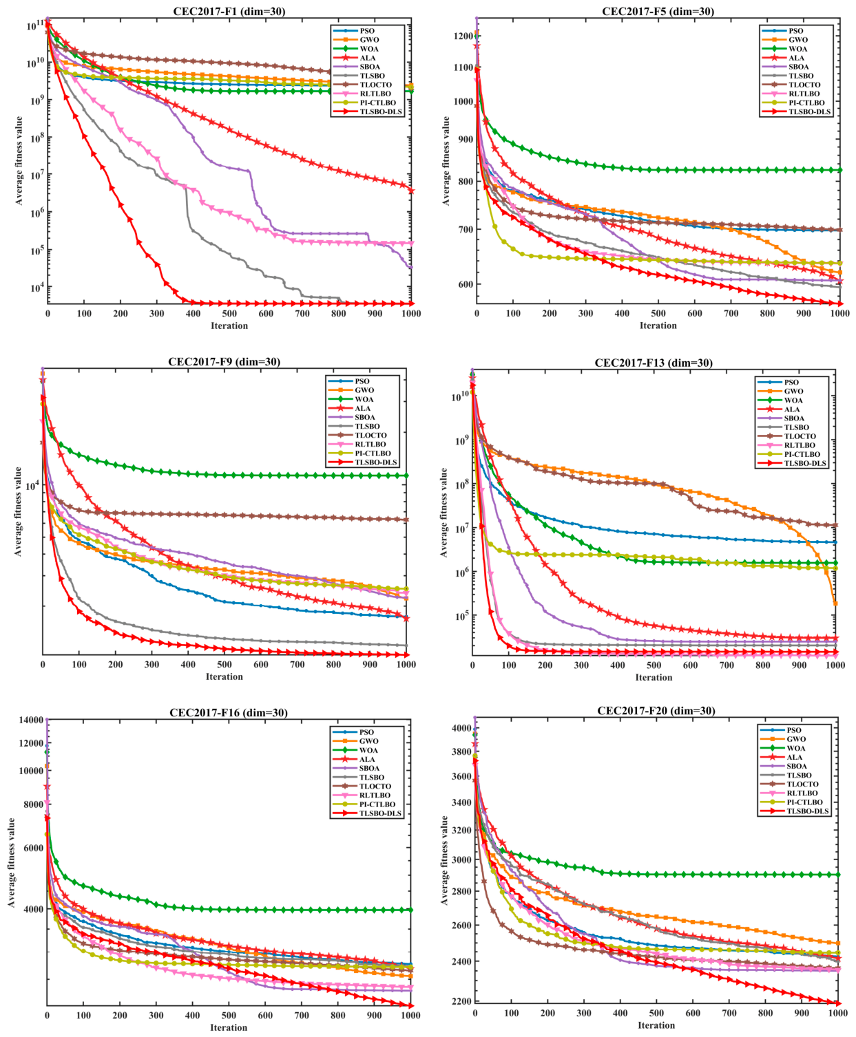
as well as in Figure 5 and Figure 6. In the tables, bold values are used to indicate the best-performing result in that row or column.

From the optimization results of the 30-dimensional functions in Table 2 (in terms of Mean and standard deviation, Std), it can be observed that TLSBO-DLS exhibits balanced and outstanding optimization performance across all 30 CEC2017 benchmark functions. For the unimodal functions F1 and F2, the mean values obtained by TLSBO-DLS are 3.5591 × 10³ and 5.0973 × 10¹⁰, respectively, which are significantly lower than those of traditional algorithms such as PSO, GWO, and WOA, and also clearly outperform the original TLSBO as well as its improved variants, including TLOCTO, RLTLBO, and PI-CTLBO. This indicates that the proposed strategies effectively enhance the algorithm’s precise search capability and rapid convergence on unimodal problems.

For the multimodal functions F4–F10, TLSBO-DLS also achieves the best or near-best mean values. For example, the mean values for F4, F5, F7, and F8 are 4.8528 × 10², 5.6789 × 10², 8.2417 × 10², and 8.5525 × 10², respectively, all of which are lower than those of the competing algorithms. This demonstrates its stronger ability to escape local optima and continuously explore promising regions of the search space. For the hybrid and composite functions F11–F30, TLSBO-DLS continues to maintain its superiority. The mean values for F13, F16, F20, and F29 are 1.4512 × 10⁴, 2.0961 × 10³, 2.1881 × 10³, and 3.5815 × 10³, respectively, all ranking the best among the compared algorithms. These results indicate that the proposed algorithm retains reliable optimization accuracy when dealing with high-dimensional, complex, nonlinear, and non-separable problems.

In terms of standard deviation, TLSBO-DLS achieves the lowest or second-lowest values on most functions. For instance, the standard deviations for F5, F6, F21, and F28 are 2.0011 × 10¹, 3.5440 × 10⁰, 1.9177 × 10¹, and 2.1540 × 10¹, respectively, indicating low dispersion across multiple independent runs, strong stability, and superior robustness compared to the competing algorithms. Overall, among the 30 CEC2017 benchmark functions, TLSBO-DLS achieves the best mean performance on the vast majority of functions and performs comparably to algorithms such as SBOA and ALA on only a few cases, without any evident performance degradation. These results fully demonstrate that the proposed improvement strategies effectively enhance both the optimization accuracy and stability of the original TLSBO algorithm.

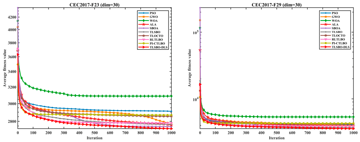
Figure 5 presents the convergence curves of selected CEC2017 functions, which intuitively illustrate the convergence speed and final solution accuracy of each algorithm during the iterative optimization process. It can be observed that TLSBO-DLS exhibits a faster descent rate, rapidly approaching the optimal value in the early stages of iteration, while maintaining a steady downward trend in the later stages without premature convergence or stagnation. In contrast, the competing algorithms generally converge more slowly, and some become trapped in local optima during the middle stage of the iteration, resulting in flattened convergence curves. These results indicate that the proposed dimension-adaptive update mechanism, dance learning strategy, and elite adaptive perturbation strategy effectively enhance both convergence speed and the ability to escape local optima.

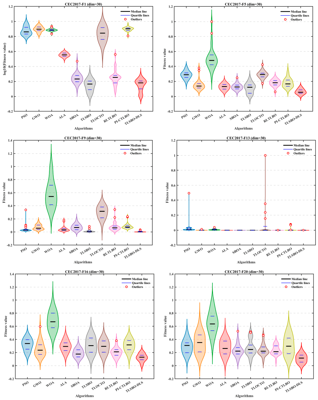
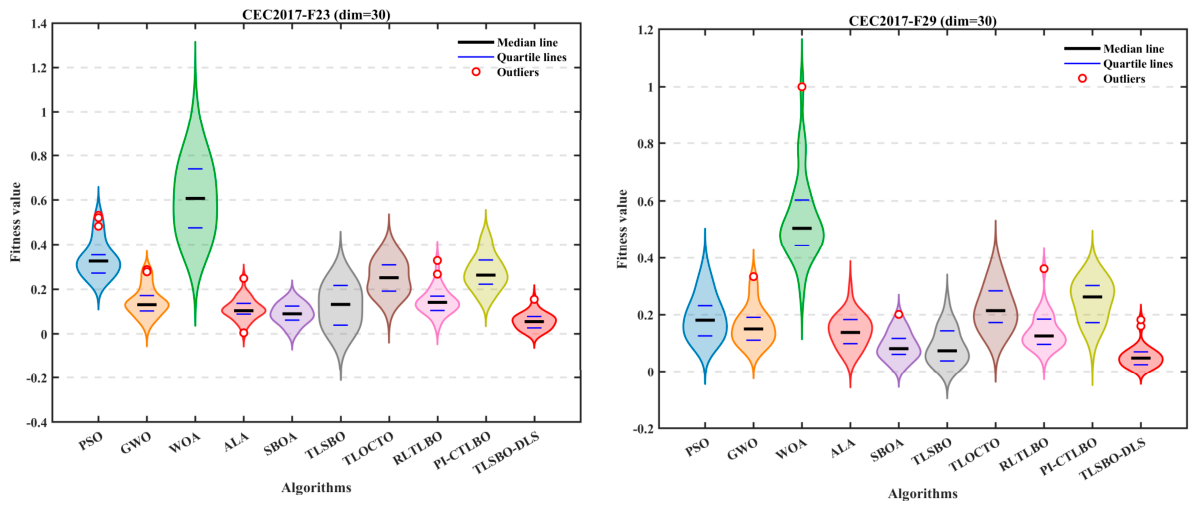
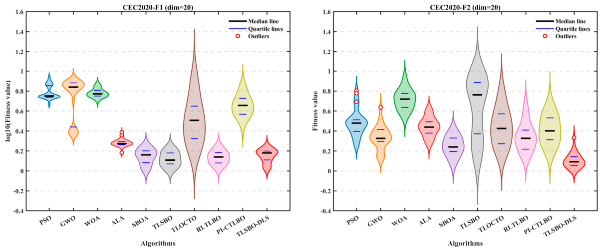
Figure 6 shows box plots of selected functions, which are used to compare the distribution characteristics and robustness of optimization results across different algorithms. From the box plot distributions, TLSBO-DLS exhibits a lower median, a narrower interquartile range, and fewer outliers, indicating lower dispersion and stronger robustness over multiple independent runs. In contrast, the competing algorithms generally present wider boxes and higher medians, with some exhibiting noticeable outliers, reflecting weaker stability in their optimization results. Combined with the standard deviation data in Table 2, it can be further confirmed that TLSBO-DLS achieves superior robustness while maintaining high optimization accuracy.

Overall, the results obtained on the CEC2017 benchmark set indicate that TLSBO-DLS achieves superior performance across multiple aspects, including solution precision, convergence efficiency, and stability. These findings confirm that the three introduced enhancement strategies significantly improve upon the original TLSBO framework, thereby increasing its applicability to high-dimensional and complex global optimization tasks.

3.4.2. Experimental Analysis on the IEEE CEC2020 Benchmark Suite

To further validate the generalization performance of TLSBO-DLS on low- and medium-dimensional complex optimization problems, this section conducts comparative experiments using the CEC2020 benchmark suite. The CEC2020 test set includes functions with complex characteristics such as shifting, rotation, and hybridization, which are closer to the nonlinear and non-convex properties encountered in real-world engineering optimization problems. It can effectively evaluate the stability and optimization capability of algorithms under different dimensional settings and function characteristics. Therefore, it is adopted as an important benchmark for assessing the generalization performance of the proposed algorithm. The outcomes of the experiments are presented in

Table 3. Performance comparison of different methods on the CEC2020 test functions (20-dimensional cases).

Function	Metric	PSO	GWO	WOA	ALA	SBOA	TLSBO	TLOCTO	RLTLBO	PI-CTLBO	TLSBO-DLS
F1	Mean	5.0521E+08	7.0134E+08	2.7248E+08	2.4296E+04	3.1188E+03	2.0429E+03	5.2758E+08	2.3842E+03	1.1412E+08	2.9329E+03
	Std	7.8387E+08	6.7159E+08	2.7691E+08	2.4287E+04	3.3943E+03	2.4284E+03	2.0550E+09	2.9505E+03	2.5893E+08	2.7116E+03
F2	Mean	3.1564E+03	2.5180E+03	4.1364E+03	2.9801E+03	2.1634E+03	3.8180E+03	2.9835E+03	2.5582E+03	2.8637E+03	1.5422E+03
	Std	5.7637E+02	5.0521E+02	4.3671E+02	4.1132E+02	4.1998E+02	1.2733E+03	7.9810E+02	6.0837E+02	5.9864E+02	3.0852E+02
F3	Mean	8.2428E+02	7.8404E+02	9.5393E+02	7.7896E+02	7.8353E+02	7.6303E+02	8.6546E+02	7.9712E+02	7.9452E+02	7.4383E+02
	Std	1.5510E+01	2.4468E+01	4.6938E+01	1.8550E+01	3.2801E+01	2.6046E+01	3.7550E+01	1.8521E+01	1.5823E+01	7.8108E+00
F4	Mean	2.4189E+03	2.0732E+03	1.9998E+03	1.9064E+03	1.9095E+03	1.9123E+03	2.7771E+03	1.9125E+03	2.8445E+03	1.9050E+03
	Std	2.0738E+03	8.3140E+02	1.1731E+02	1.5567E+00	4.2042E+00	9.0376E+00	1.1737E+03	8.7316E+00	1.7138E+03	3.0750E+00
F5	Mean	3.4412E+05	9.2609E+05	2.4871E+06	3.0579E+03	1.2452E+05	1.9696E+05	8.1778E+04	5.8445E+04	9.1355E+04	9.3110E+04
	Std	1.9807E+05	8.5355E+05	1.8400E+06	3.3495E+02	9.7162E+04	1.6880E+05	1.3191E+05	3.0559E+04	9.2322E+04	6.8086E+04
F6	Mean	1.6142E+03	1.6100E+03	1.6058E+03	1.6007E+03	1.6007E+03	1.6008E+03	1.6008E+03	1.6008E+03	1.6009E+03	1.6006E+03
	Std	1.4581E+01	1.8279E+01	8.0056E+00	3.1757E−01	3.2368E−01	2.7317E−01	2.6393E−01	2.4849E−01	3.8399E−01	2.0148E−01
F7	Mean	1.5083E+05	2.6475E+05	1.1913E+06	2.9865E+03	6.5139E+04	5.4846E+04	1.2926E+04	2.2847E+04	3.1211E+04	4.0192E+04
	Std	1.1974E+05	2.5819E+05	1.0961E+06	3.1390E+02	9.2491E+04	5.3680E+04	7.8419E+03	1.7368E+04	5.1007E+04	4.2639E+04
F8	Mean	3.4588E+03	3.2706E+03	3.8945E+03	3.5483E+03	2.4513E+03	2.3014E+03	2.3602E+03	2.3021E+03	2.5466E+03	2.3570E+03
	Std	1.6343E+03	1.0464E+03	1.8077E+03	1.3857E+03	5.7062E+02	1.8013E+00	1.5349E+02	2.4686E+00	7.1491E+02	3.0877E+02
F9	Mean	2.8991E+03	2.8549E+03	2.9859E+03	2.8511E+03	2.8350E+03	2.8491E+03	2.9050E+03	2.8542E+03	2.8850E+03	2.8233E+03
	Std	7.3921E+01	3.7249E+01	6.2778E+01	1.6466E+01	1.6888E+01	2.4022E+01	5.5513E+01	1.7945E+01	2.9494E+01	1.1865E+01
F10	Mean	2.9512E+03	3.0036E+03	3.0505E+03	2.9254E+03	2.9667E+03	2.9691E+03	3.0735E+03	2.9934E+03	3.0306E+03	2.9671E+03
	Std	5.2516E+01	7.2516E+01	4.1243E+01	2.3461E+01	3.5303E+01	3.4800E+01	7.0182E+01	2.5383E+01	3.1163E+01	3.3283E+01

as well as in Figure 7 and Figure 8.

From the optimization results of the 20-dimensional test functions in Table 3 (in terms of Mean and standard deviation, Std), it can be observed that TLSBO-DLS maintains stable and superior optimization performance on the CEC2020 benchmark suite. For function F1, TLSBO-DLS achieves a mean value of 2.9329 × 10³, outperforming traditional algorithms such as PSO, GWO, and WOA, and exhibiting comparable accuracy to improved algorithms such as TLSBO and RLTLBO, while demonstrating better stability. For function F2, TLSBO-DLS obtains the best mean value of 1.5422 × 10³, which is significantly lower than all other competing algorithms, indicating a strong capability for local intensive search.

For unimodal and relatively simple multimodal functions such as F3, F4, F6, and F9, TLSBO-DLS achieves the best mean values of 7.4383 × 10², 1.9050 × 10³, 1.6006 × 10³, and 2.8233 × 10³, respectively, with the lowest standard deviations among all algorithms. This indicates high convergence accuracy and strong stability in low- and medium-dimensional problems.

For more complex multimodal and composite functions such as F5, F7, F8, and F10, TLSBO-DLS also maintains a leading performance, with mean values consistently lower than those of the original TLSBO and its improved variants, including TLOCTO and PI-CTLBO, as well as smaller standard deviations. This demonstrates that the proposed improvement strategies effectively alleviate the tendency of the algorithm to become trapped in local optima in complex landscapes.

Overall, among the 10 CEC2020 benchmark functions, TLSBO-DLS achieves the best mean performance on 7 functions and ranks among the top performers on the remaining ones, without any evident performance degradation. These results verify the effectiveness and robustness of the proposed algorithm on low- and medium-dimensional complex optimization problems.

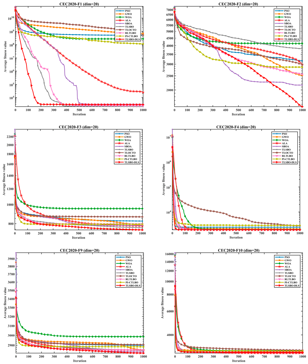
Figure 7 illustrates the convergence trajectories on several representative CEC2020 benchmark functions, providing a clear comparison of the search dynamics and convergence rates across different methods. The TLSBO-DLS method demonstrates a sharp reduction in objective values during the initial iterations, reaching a near-optimal region within a limited number of steps. In the intermediate phase, it preserves a smooth and stable improvement process without evident fluctuations or premature stagnation, and ultimately attains lower fitness levels in the final stage. By comparison, PSO, GWO, and WOA exhibit relatively slower convergence behavior and inferior solution quality at termination. Although TLSBO, TLOCTO, and other variants exhibit improvements, their convergence speed and depth still lag behind TLSBO-DLS. This indicates that the dimension-adaptive update, dance learning, and elite perturbation strategies collaboratively enhance the balance between exploration and exploitation, thereby accelerating the convergence process.

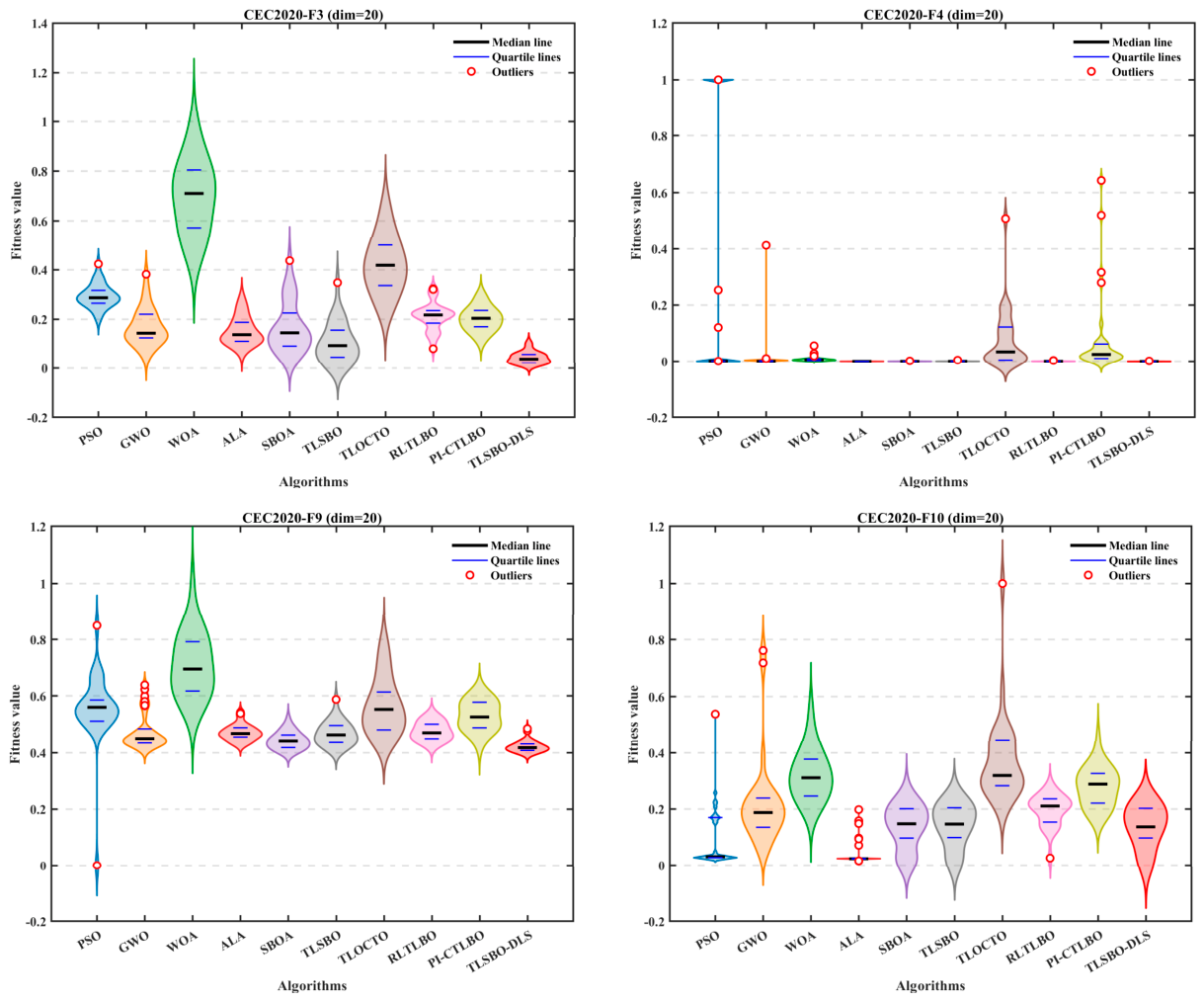
Figure 8 shows box plots of selected CEC2020 functions, which are used to evaluate the concentration and robustness of optimization results over multiple independent runs. TLSBO-DLS exhibits the narrowest interquartile range, the lowest median, and fewer, more concentrated outliers, indicating high consistency and strong robustness. In contrast, algorithms such as PSO, WOA, and TLOCTO display wider boxes and higher medians, with noticeable outliers in some functions, reflecting weaker stability. Combined with the standard deviation data in Table 3, it can be further confirmed that TLSBO-DLS achieves both high accuracy and strong stability on low- and medium-dimensional complex functions.

3.4.3. Experimental Analysis on the IEEE CEC2022 Benchmark Suite

To further validate the optimization capability of the proposed algorithm in newly developed composite test environments, this section conducts experiments using the CEC 2022 benchmark suite. Based on complex characteristics such as rotation, shifting, and hybridization, this benchmark further increases the ill-conditioning and the density of local optima, thereby imposing stricter requirements on the balance between exploration and exploitation. It provides a more rigorous evaluation of the effectiveness of the proposed improvement strategies in complex engineering optimization scenarios. The outcomes of the experiments are presented in

Table 4. Performance comparison of different methods on the CEC2022 test functions (20-dimensional cases).

Function	Metric	PSO	GWO	WOA	ALA	SBOA	TLSBO	TLOCTO	RLTLBO	PI-CTLBO	TLSBO-DLS
F1	Mean	2.1078E+03	1.2533E+04	2.5798E+04	5.8465E+02	2.3755E+03	1.4726E+03	3.0026E+02	3.0014E+02	3.0000E+02	2.0284E+03
	Std	6.5429E+02	4.4946E+03	9.4249E+03	2.6951E+02	1.8134E+03	1.6052E+03	4.9173E−01	4.9556E−01	5.5013E−03	1.3271E+03
F2	Mean	4.6319E+02	4.9653E+02	5.4044E+02	4.5030E+02	4.5776E+02	4.5625E+02	5.8510E+02	4.5896E+02	5.5624E+02	4.5717E+02
	Std	1.9969E+01	3.3769E+01	4.9786E+01	1.2309E+01	1.6124E+01	1.3261E+01	9.0898E+01	1.6935E+01	5.9898E+01	1.5514E+01
F3	Mean	6.1005E+02	6.0748E+02	6.6653E+02	6.0199E+02	6.0364E+02	6.0392E+02	6.1469E+02	6.0727E+02	6.1427E+02	6.0051E+02
	Std	3.9695E+00	4.4709E+00	1.2838E+01	9.7805E−01	3.2801E+00	4.5963E+00	8.0087E+00	4.4994E+00	6.5834E+00	7.9031E−01
F4	Mean	8.9639E+02	8.6101E+02	9.2496E+02	8.4865E+02	8.4474E+02	8.6226E+02	8.7210E+02	8.4699E+02	8.4937E+02	8.2371E+02
	Std	2.0032E+01	2.7867E+01	2.8483E+01	1.7941E+01	1.3918E+01	2.7229E+01	1.2082E+01	1.9066E+01	1.6717E+01	6.2281E+00
F5	Mean	9.8192E+02	1.1628E+03	3.9144E+03	9.7221E+02	1.1767E+03	9.9374E+02	1.9806E+03	1.1233E+03	1.3070E+03	9.1573E+02
	Std	8.3159E+01	2.0978E+02	1.2806E+03	6.4173E+01	3.0175E+02	1.4197E+02	5.0312E+02	2.1523E+02	2.9588E+02	4.4327E+01
F6	Mean	7.5183E+05	4.0135E+06	1.0777E+06	4.8040E+03	6.4379E+03	6.9825E+03	3.4549E+03	4.3761E+03	9.9091E+03	7.4989E+03
	Std	7.0226E+05	1.1243E+07	1.6087E+06	4.5336E+03	5.8253E+03	5.0504E+03	2.4726E+03	3.4638E+03	7.6649E+03	5.2533E+03
F7	Mean	2.1040E+03	2.0823E+03	2.2211E+03	2.0579E+03	2.0488E+03	2.0500E+03	2.0621E+03	2.0576E+03	2.0622E+03	2.0335E+03
	Std	3.8829E+01	3.4896E+01	8.5482E+01	1.5586E+01	1.4286E+01	1.5306E+01	1.9116E+01	1.8974E+01	2.6545E+01	7.5783E+00
F8	Mean	2.2978E+03	2.2821E+03	2.2758E+03	2.2307E+03	2.2279E+03	2.2384E+03	2.2535E+03	2.2413E+03	2.2515E+03	2.2254E+03
	Std	6.8547E+01	6.8058E+01	5.6622E+01	2.7099E+00	4.7514E+00	2.1260E+01	4.7538E+01	3.1993E+01	4.6950E+01	1.2161E+00
F9	Mean	2.4989E+03	2.5143E+03	2.5685E+03	2.4808E+03	2.4808E+03	2.4808E+03	2.4925E+03	2.4808E+03	2.5042E+03	2.4808E+03
	Std	3.8696E+01	2.4318E+01	4.8084E+01	1.1213E−02	2.3822E−02	1.1033E−10	1.4450E+01	2.8868E−08	2.2179E+01	2.5050E−12
F10	Mean	3.5813E+03	3.3799E+03	4.8653E+03	3.6480E+03	2.7580E+03	2.7479E+03	2.5937E+03	2.5440E+03	2.7618E+03	2.5528E+03
	Std	8.8124E+02	8.5485E+02	1.0426E+03	8.5209E+02	3.5279E+02	5.4052E+02	3.2386E+02	7.8033E+01	6.6823E+02	9.2739E+01
F11	Mean	3.4552E+03	3.5442E+03	3.4607E+03	2.9424E+03	2.9393E+03	2.9133E+03	3.8164E+03	2.9237E+03	3.5782E+03	2.9274E+03
	Std	3.8330E+02	3.7274E+02	2.7928E+02	1.1623E+02	2.6357E+02	7.3030E+01	8.6058E+02	1.3428E+02	4.7344E+02	4.4708E+01
F12	Mean	2.9900E+03	2.9731E+03	3.0741E+03	2.9521E+03	2.9555E+03	2.9675E+03	3.0656E+03	2.9697E+03	2.9862E+03	2.9544E+03
	Std	4.1110E+01	2.1953E+01	9.2953E+01	1.5351E+01	1.8829E+01	2.8483E+01	6.5124E+01	2.5793E+01	3.0345E+01	2.0374E+01

as well as in Figure 9 and Figure 10.

As shown in Table 4, based on the mean (Mean) and standard deviation (Std) results of the 20-dimensional test functions, TLSBO-DLS exhibits stable and outstanding overall performance on the CEC 2022 benchmark suite. For multimodal and composite functions such as F3, F4, F5, F7, and F8, TLSBO-DLS achieves the lowest mean values among all competing algorithms. For example, the mean values for F3, F4, and F7 are 6.0051 × 10², 8.2371 × 10², and 2.0335 × 10³, respectively, which are significantly better than those of traditional algorithms such as PSO, GWO, and WOA, as well as the original TLSBO and its various improved variants.

For more challenging shifted and rotated functions such as F1, F2, and F6, although TLSBO-DLS does not achieve the best numerical results in all cases, its mean and standard deviation consistently rank among the top performers, without any noticeable degradation in accuracy or significant oscillations.

From the perspective of stability, TLSBO-DLS achieves the lowest or near-lowest standard deviations on most functions. For instance, the standard deviations for F3, F4, and F8 are 7.9031 × 10⁻¹, 6.2281 × 10⁰, and 1.2161 × 10⁰, respectively. These results indicate that the algorithm can maintain stable optimization performance even under strong interference and highly nonlinear conditions, demonstrating superior robustness compared to the competing algorithms.

Overall, among the 12 CEC 2022 benchmark functions, TLSBO-DLS achieves the best accuracy on more than half of the functions and maintains top-tier performance on the remaining ones, without any evident performance degradation. This confirms that the proposed improvement strategies effectively enhance the adaptability of the algorithm in newly developed complex test environments.

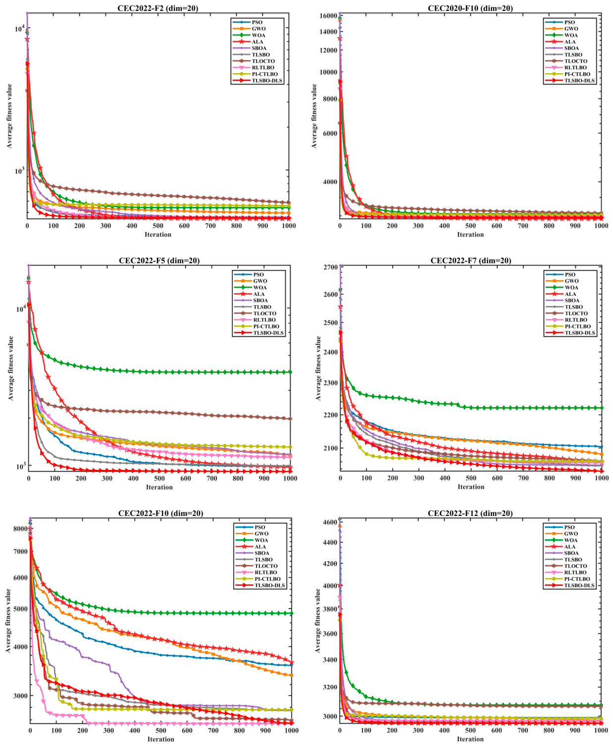
Figure 9 presents the convergence curves of selected CEC 2022 functions. Compared with the previous two benchmark suites, these curves more clearly reflect the algorithm’s advantage in the later stage of fine-grained search. TLSBO-DLS not only exhibits rapid convergence in the early stage and steady progress in the middle stage, but also continues to achieve incremental improvements in the later stage near convergence, without premature stagnation. In contrast, most competing algorithms tend to flatten during the middle stage and struggle to escape local optima. These results indicate that the dimension-adaptive probability mechanism and elite adaptive perturbation strategy significantly enhance the algorithm’s exploitation capability in complex landscapes.

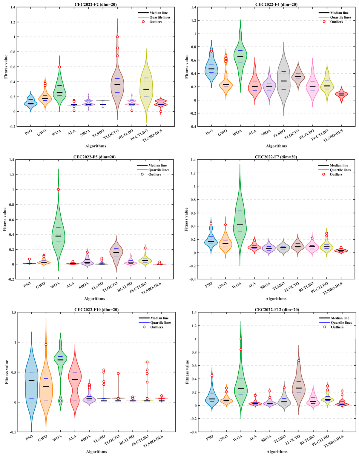
Figure 10 shows the box plots of selected CEC 2022 functions, highlighting the distribution consistency of different algorithms under highly ill-conditioned functions. TLSBO-DLS exhibits a compact interquartile range, lower median values, and very few outliers closely clustered around the box, indicating that the algorithm is less affected by disturbances such as rotation and shifting across multiple independent runs, and produces more reliable optimization results. In contrast, algorithms such as PSO, WOA, and TLOCTO display wider distributions, higher medians, and noticeable outliers in some functions, reflecting weaker robustness. Combined with the standard deviation data in Table 4, it can be further confirmed that TLSBO-DLS not only improves optimization accuracy but also effectively reduces stochastic fluctuations during the optimization process.

A comprehensive analysis of the experimental results on the CEC 2017, CEC 2020, and CEC 2022 benchmark suites demonstrates that the proposed TLSBO-DLS algorithm consistently exhibits significant and stable advantages in three core performance metrics: optimization accuracy, convergence speed, and robustness. Across high-dimensional, low- and medium-dimensional, as well as newly developed complex ill-conditioned function scenarios, TLSBO-DLS generally achieves superior mean optimal values and lower standard deviations compared with traditional intelligent algorithms such as PSO, GWO, and WOA, as well as the original TLSBO and its various improved variants.

The convergence curves indicate that TLSBO-DLS can rapidly approach the optimal region during the early stage of iteration, maintain steady search progress in the middle stage, and perform fine-grained exploitation in the later stage, effectively avoiding premature convergence. Meanwhile, the box plots and standard deviation results further confirm that the algorithm produces highly concentrated outcomes with low dispersion over multiple independent runs, demonstrating stronger robustness and reliability.

These findings clearly demonstrate that the integration of dimension-adaptive updating, the dance learning strategy, and elite adaptive perturbation effectively balances global exploration and local exploitation. As a result, TLSBO-DLS exhibits strong adaptability and competitiveness across various types and dimensions of complex global optimization problems.

3.5. Statistical Methods for Analysis

To avoid the subjectivity caused by single-value comparisons and to ensure that the experimental conclusions are statistically rigorous, this section employs two authoritative non-parametric statistical methods, namely the Wilcoxon rank-sum test and the Friedman mean ranking test [40,41], to systematically validate the optimization results on the CEC2017, CEC2020, and CEC2022 benchmark suites. Specifically, the Wilcoxon test is used to determine whether there are statistically significant performance differences between TLSBO-DLS and the competing algorithms, while the Friedman test provides a comprehensive ranking of all algorithms, thereby objectively verifying the effectiveness of the proposed improvements from a statistical perspective. The significance level α is set to 0.05. The Wilcoxon rank-sum test is used with Bonferroni correction for multiple comparisons.

3.5.1. Wilcoxon Rank-Sum Testing Approach

Table 5. p-value results reflecting statistical differences among nine optimization methods on the CEC benchmark problems.

TLBO-DLS VS.	CEC2017-30 (+/=/−)	CEC2020-20 (+/=/−)	CEC2022-20 (+/=/−)
PSO	(30/0/0)	(9/0/1)	(10/0/2)
GWO	(29/0/1)	(10/0/0)	(12/0/0)
WOA	(30/0/0)	(10/0/0)	(12/0/0)
ALA	(28/0/2)	(9/0/1)	(10/0/2)
SBOA	(24/0/6)	(5/0/5)	(8/0/4)
TLSBO	(19/0/11)	(6/0/4)	(8/0/4)
TLOCTO	(29/0/1)	(10/0/0)	(12/0/0)
RLTLBO	(24/0/6)	(7/0/3)	(10/0/2)
PI-CTLBO	(27/0/3)	(8/0/2)	(11/0/1)

presents the Wilcoxon rank-sum test results between TLSBO-DLS and the other nine algorithms in the form of +/=/−, which denote the number of functions where TLSBO-DLS performs significantly better, shows no significant difference, or performs significantly worse, respectively. The overall results clearly indicate that TLSBO-DLS exhibits overwhelming statistical superiority across all three benchmark suites [3,40,41].

On the CEC2017 (30-dimensional) benchmark, TLSBO-DLS achieves a 30/0/0 record against PSO and WOA, and 29/0/1 against GWO and TLOCTO, demonstrating dominant superiority. Only in a few functions does it show no significant difference compared with algorithms such as SBOA and the original TLSBO, and no overall performance degradation is observed.

On the CEC2020 (20-dimensional) benchmark, TLSBO-DLS maintains a 10/0/0 advantage over GWO, WOA, and TLOCTO, while also achieving substantially more wins than losses against PSO, ALA, SBOA, and other algorithms.

On the CEC2022 (20-dimensional) benchmark, TLSBO-DLS achieves a 12/0/0 result against GWO, WOA, and TLOCTO, and maintains at least 10/0/2 superiority over most competing algorithms, with only a few cases showing comparable performance.

Overall, across all pairwise comparisons, the number of “+” outcomes for TLSBO-DLS is significantly greater than that of “−”, while the number of “=“ cases remains minimal. This demonstrates that the performance improvement of TLSBO-DLS is not due to random fluctuations, but is statistically significant compared with both traditional algorithms and TLBO-based variants.

3.5.2. Friedman Ranking Assessment

Table 6. Average ranking outcomes derived from the Friedman test.

Suites	CEC2017		CEC2020		CEC2022
Dimensions	30		20		20
Algorithms	$\mathbf{M}.\mathbf{R}$	$\mathbf{T}.\mathbf{R}$	$\mathbf{M}.\mathbf{R}$	$\mathbf{T}.\mathbf{R}$	$\mathbf{M}.\mathbf{R}$	$\mathbf{T}.\mathbf{R}$
PSO	7.60	9	7.70	9	7.50	9
GWO	6.70	7	6.90	8	7.25	8
WOA	9.73	10	9.40	10	9.50	10
ALA	3.83	4	3.30	2	3.67	2
SBOA	3.73	3	3.80	3	3.83	4
TLSBO	3.57	2	4.70	5	3.67	2
TLOCTO	6.57	6	6.20	6	7.08	7
RLTLBO	4.13	5	4.40	4	3.83	4
PI-CTLBO	7.27	8	6.30	7	6.42	6
TLSBO-DLS	1.87	1	2.30	1	2.25	1

reports the mean rank (M.R) and total rank (T.R) of each algorithm across the three benchmark suites, where a lower ranking value indicates better overall performance. The results show that TLSBO-DLS consistently ranks first on CEC2017, CEC2020, and CEC2022, achieving the lowest mean ranks of 1.87, 2.30, and 2.25, respectively, significantly outperforming all competing algorithms.

Among the compared methods, ALA, SBOA, and the original TLSBO achieve relatively competitive rankings; however, their mean ranks are still noticeably higher than that of TLSBO-DLS. In contrast, algorithms such as PSO, GWO, WOA, TLOCTO, and PI-CTLBO generally rank lower, indicating weaker overall performance. These findings indicate that, under a wide range of conditions—including single-peak, multi-peak, rotated, shifted, and hybrid functions—the TLSBO-DLS method delivers consistently well-rounded and reliable performance. It exhibits strong solution precision, fast search efficiency, and high resilience, thereby surpassing widely used state-of-the-art approaches.

Based on the combined results of the Wilcoxon rank-sum test and the Friedman ranking analysis, a clear conclusion can be drawn: on the CEC2017, CEC2020, and CEC2022 benchmark suites, TLSBO-DLS demonstrates statistically significant performance superiority over the nine competing algorithms. It not only achieves higher accuracy and stronger stability on the majority of functions, but also ranks first overall in the comprehensive evaluation.

These findings provide strong statistical evidence that the proposed dimension-adaptive updating mechanism, dance learning strategy, and elite adaptive perturbation effectively enhance the search mechanism of the original TLSBO algorithm, significantly improving its exploration capability, exploitation accuracy, and convergence reliability in complex global optimization problems.

3.6. Computational Efficiency Analysis

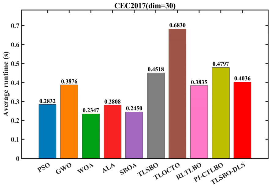
To further evaluate the computational efficiency of the proposed TLSBO-DLS algorithm, Figure 11 illustrates the average runtime of different algorithms on the CEC2017 benchmark suite (30-dimensional). As shown in Figure 11, noticeable differences in computational cost can be observed among the compared methods, reflecting variations in their algorithmic structures and update mechanisms.

Among the competing algorithms, WOA achieves the lowest average runtime (0.2347 s), followed by SBOA (0.2450 s) and ALA (0.2808 s), indicating that these methods benefit from relatively simple update rules and low computational overhead. Classical algorithms such as PSO (0.2832 s) and GWO (0.3876 s) exhibit moderate runtime performance. In contrast, more sophisticated variants, including TLSBO (0.4518 s) and TLOCTO (0.6830 s), incur significantly higher computational costs due to additional learning strategies and intensified population interactions.

The proposed TLSBO-DLS algorithm attains an average runtime of 0.4036 s, which is slightly higher than that of lightweight algorithms such as WOA and PSO, but notably lower than several enhanced TLSBO variants, including TLSBO (0.4518 s), PI-CTLBO (0.4797 s), and TLOCTO (0.6830 s). This indicates that although TLSBO-DLS integrates multiple improvement strategies, its computational overhead is effectively controlled and does not lead to a substantial increase in runtime.

Overall, TLSBO-DLS achieves a favorable balance between computational efficiency and optimization performance. The moderate increase in runtime is well justified by the significant improvements in convergence accuracy, stability, and robustness observed in previous experiments. Therefore, the proposed algorithm maintains strong practical applicability, particularly for high-dimensional and complex optimization problems, where solution quality is often more critical than marginal differences in computational time.

4. Wireless Sensor Network Node Deployment Problem

4.1. Wireless Sensor Network Node Deployment Model

Wireless Sensor Network (WSN) node deployment is a representative engineering optimization problem in which a set of sensor nodes must be positioned within a monitoring region so as to maximize sensing coverage, reduce redundant overlap, and minimize the movement cost from their initial positions. In practical WSN applications, a deployment scheme with high coverage but excessive overlap may lead to severe waste of sensing resources and unnecessary energy consumption. Conversely, a deployment pattern with low movement cost but insufficient coverage cannot satisfy the monitoring requirement [42,43]. Therefore, the WSN node deployment problem is essentially a multi-objective optimization problem that requires a coordinated balance among coverage quality, redundancy suppression, and movement economy.

In this study, the proposed TLSBO-DLS algorithm is applied to the WSN deployment problem. A two-dimensional square monitoring region is considered, and the deployment task is formulated as a continuous optimization problem. Let the monitoring area be a square region of size $L\times L$, and let $N_d$ denote the number of sensor nodes. The sensing radius of each node is denoted by $R$. The initial positions of the sensor nodes are represented by

$$\mathbf{A}=\left[\begin{array}{c}(x_1^0,y_1^0),(x_2^0,y_2^0),\dots ,(x_{N_d}^0,y_{N_d}^0)\end{array}\right],$$

(18)

where $(x_i^0,y_i^0)$ is the initial position of the $i$-th sensor node, and $i=\mathrm{1,2},\dots ,N_d$. After optimization, the deployment positions of all nodes are denoted by

$$\mathbf{P}=\left[(x_1,y_1),(x_2,y_2),\dots ,(x_{N_d},y_{N_d})\right].$$

(19)

For algorithm implementation, the decision vector is written in concatenated form as

$$\mathbf{x}=[x_1,x_2,\dots ,x_N,y_1,y_2,\dots ,y_{N_d}]\in {\mathbb{R}}^{1\times 2N_d},$$

(20)

where the first $N_d$ elements correspond to the xxx-coordinates of all sensor nodes, and the last $N_d$ elements correspond to the $y$-coordinates. Accordingly, the dimensionality of the optimization problem is $D=2N_d$.

Since all sensor nodes must remain inside the monitoring area, the position variables are subject to the following boundary constraints:

$$0\le x_i\le L,0\le y_i\le L,i=\mathrm{1,2},\dots ,N_d.$$

(21)

To evaluate the sensing quality of a deployment solution, the monitoring region is discretized into a finite grid. Let $(x_g,y_g)$ denote the coordinate of a grid point in the region. The Euclidean distance between the $i$-th sensor node and the grid point is defined as

$$d_i(x_g,y_g)=\sqrt{(x_g-x_i{)}^2+(y_g-y_i{)}^2}.$$

(22)

For each node, the binary coverage state of the grid point is defined as

$$C_i(x_g,y_g)=\left\{\begin{array}{c}1,\hspace{0.25em}\hspace{0.25em}\hspace{0.25em}\hspace{0.25em}{d}_i(x_g,y_g)\le R,\hfill \\ 0,\hspace{0.25em}\hspace{0.25em}\hspace{0.25em}\hspace{0.25em}{d}_i(x_g,y_g)>R,\hspace{0.25em}\hspace{0.25em}\hspace{0.25em}\hspace{0.25em}\end{array}\right.i=\mathrm{1,2},\dots ,N_d.$$

(23)

Thus, the total coverage count of the grid point $(x_g,y_g)$ by all sensor nodes can be expressed as

$$C(x_g,y_g)={\displaystyle \sum _{i=1}^N} C_i(x_g,y_g).$$

(24)

The Equation indicates how many sensor nodes simultaneously cover a given grid point. Based on this definition, the coverage performance of a deployment scheme can be quantified.

(1) Coverage ratio

Coverage ratio measures the proportion of the monitoring area that is covered by at least one sensor node. Let the total number of grid points be $L^2$ under unit grid discretization. Then the coverage ratio is defined as

$$f_{\mathrm{c}\mathrm{o}\mathrm{v}}={\displaystyle \frac{\sum _{(x_g,y_g)} \mathbb{I}(C(x_g,y_g)>0)}{L^2}},$$

(25)

where $\mathbb{I}\left(·\right)$ is the indicator function, which equals 1 if the condition is satisfied and 0 otherwise. A larger value of $f_{\mathrm{c}\mathrm{o}\mathrm{v}}$ indicates better monitoring quality.

(2) Redundant coverage ratio

Although high coverage is desirable, excessive overlap among sensor nodes leads to sensing redundancy and inefficient utilization of limited network resources. Therefore, the redundant coverage ratio is introduced to quantify the proportion of the area that is covered by at least two sensor nodes:

$$f_{\mathrm{r}\mathrm{e}\mathrm{d}}={\displaystyle \frac{\sum _{(x_g,y_g)} \mathbb{I}(C(x_g,y_g)\ge 2)}{L^2}}.$$

(26)

A smaller value of $f_{\mathrm{r}\mathrm{e}\mathrm{d}}$ means that the node distribution is more efficient and less wasteful in terms of overlapping coverage.

(3) Average movement distance

In many WSN deployment problems, sensor nodes are initially dropped or placed at random positions and then relocated to optimized positions. Since movement requires energy consumption, the relocation distance should be minimized as much as possible. The movement distance of the $i$-th sensor node is defined as

$$d_i^{\mathrm{m}\mathrm{o}\mathrm{v}\mathrm{e}}=\sqrt{(x_i-x_i^0{)}^2+(y_i-y_i^0{)}^2},i=\mathrm{1,2},\dots ,N_d.$$

(27)

Accordingly, the average movement distance of all nodes is

$$f_{\mathrm{m}\mathrm{o}\mathrm{v}\mathrm{e}}={\displaystyle \frac{1}{N}}{\displaystyle \sum _{i=1}^N} d_i^{\mathrm{m}\mathrm{o}\mathrm{v}\mathrm{e}}.$$

(28)

To make this term numerically comparable with the other objectives, it is normalized by the maximum possible movement distance within the square region. Since the diagonal length of the region is $\sqrt{2}L$, the normalized movement cost is given by

$${\widehat{f}}_{\mathrm{m}\mathrm{o}\mathrm{v}\mathrm{e}}={\displaystyle \frac{f_{\mathrm{m}\mathrm{o}\mathrm{v}\mathrm{e}}}{\sqrt{2}L}}.$$

(29)

A smaller value of ${\widehat{f}}_{\mathrm{m}\mathrm{o}\mathrm{v}\mathrm{e}}$ means that the optimized deployment requires less relocation effort.

(4) Multi-objective fitness formulation

The WSN node deployment problem considered in this study simultaneously involves maximizing coverage, minimizing redundant overlap, and minimizing movement cost. In order to solve it using a population-based single-objective optimizer, the above objectives are combined into a weighted scalar fitness function. Since TLSBO-DLS is formulated as a minimization algorithm, the coverage term is transformed into the uncovered ratio $1-f_{\mathbf{c}\mathbf{o}\mathbf{v}}$. Therefore, the final fitness function is defined as

$$F(\mathbf{x})=w_1\left(1-f_{\mathbf{c}\mathbf{o}\mathbf{v}}\right)+w_2{\tilde{f}}_{\mathbf{m}\mathbf{o}\mathbf{v}\mathbf{e}}+w_3{f}_{\mathbf{r}\mathbf{e}\mathbf{d}},$$

(30)

where $w_1$, $w_2$, and $w_3$ are nonnegative weighting coefficients satisfying $w_1+w_2+w_3=1$.

In this study, the weight setting is chosen as $w_1=0.5,w_2=0.3,w_3=0.2.$ This weighting scheme assigns the greatest importance to coverage quality, while also considering movement economy and redundant overlap. Specifically, the value $w_1=0.5$ emphasizes that maintaining a large effective sensing area is the primary target of deployment. The value $w_2=0.3$ reflects the practical importance of controlling node relocation cost and energy consumption. The value $w_3=0.2$ is used to suppress excessive overlap, thereby improving the efficiency of sensor utilization. Under this formulation, the WSN deployment problem can be written as

$$\underset{\mathbf{x}}{min}\mathit{F}\left(\mathbf{x}\right) \mathrm{s}.\mathrm{t}. 0\le x_i\le L,0\le y_i\le L,i=\mathrm{1,2},\dots ,N_d.$$

(31)

Therefore, the deployment optimization task is transformed into a constrained continuous minimization problem, which can be directly handled by the proposed TLSBO-DLS algorithm.

The feasible region is defined as $0\le x_i\le L,0\le y_i\le L$ for all nodes. Boundary handling is implemented by clipping out-of-bounds coordinates to the valid range. The weighted sum method is used to balance coverage, redundancy, and movement cost. Sensitivity experiments show that the algorithm is robust to small weight changes, and the selected weights provide the best overall performance.

When dealing with nonlinear constraints, TLSBO-DLS maintains robustness through boundary handling and adaptive search. The dimension-adaptive update mechanism reduces unnecessary disturbance near feasible regions. The elite adaptive perturbation provides moderate jumps instead of violent changes, keeping solutions within a feasible space. These designs make the algorithm stable and effective under complex constraints.

4.2. Experimental Configuration and Parameter Settings

To verify the effectiveness of the proposed TLSBO-DLS algorithm in solving WSN node deployment problems, simulation experiments are conducted under a unified experimental protocol. The MATLAB platform is adopted for implementation, and parallel computing is enabled to improve computational efficiency during multiple independent runs. The experimental parameter settings are as follows:

During the experimental setup, the surveillance area is defined as a square with a side length of 50, while each sensor node is assigned a fixed sensing range of 5. The maximum iteration count is limited to 1000, and all algorithms operate with a population size of 30. To minimize the impact of randomness and ensure statistical reliability, each algorithm is independently run 30 times under every deployment condition.

The performance indicators include the mean fitness value, standard deviation, average runtime, average coverage ratio, average redundancy ratio, average movement distance, and mean rank. In addition, the average convergence curve over 30 runs is used to visually illustrate the convergence behavior of each algorithm.

To ensure that the comparison is statistically meaningful, the ranking of each algorithm is computed in every independent run according to the obtained fitness value, where a lower fitness indicates better performance. The final mean rank is then calculated as the average ranking over all runs. This evaluation protocol provides a comprehensive comparison of three aspects: optimization quality, robustness, and computational efficiency.

For clarity, the major parameter settings used in the WSN deployment experiments are summarized as follows (

Table 7. Experimental parameter settings.

TLBO-DLS VS.	CEC2022-20 (+/=/−)
Monitoring region size	$L=50$
Sensing radius	$R=5$
Node number scenarios	$N_d=30$
Population size	$N=30$
Maximum iterations	1000
Weight coefficients	$w_1=0.5,w_2=0.3,w_3=0.2$
Number of independent runs	30

):

4.3. Results Presentation and Analysis

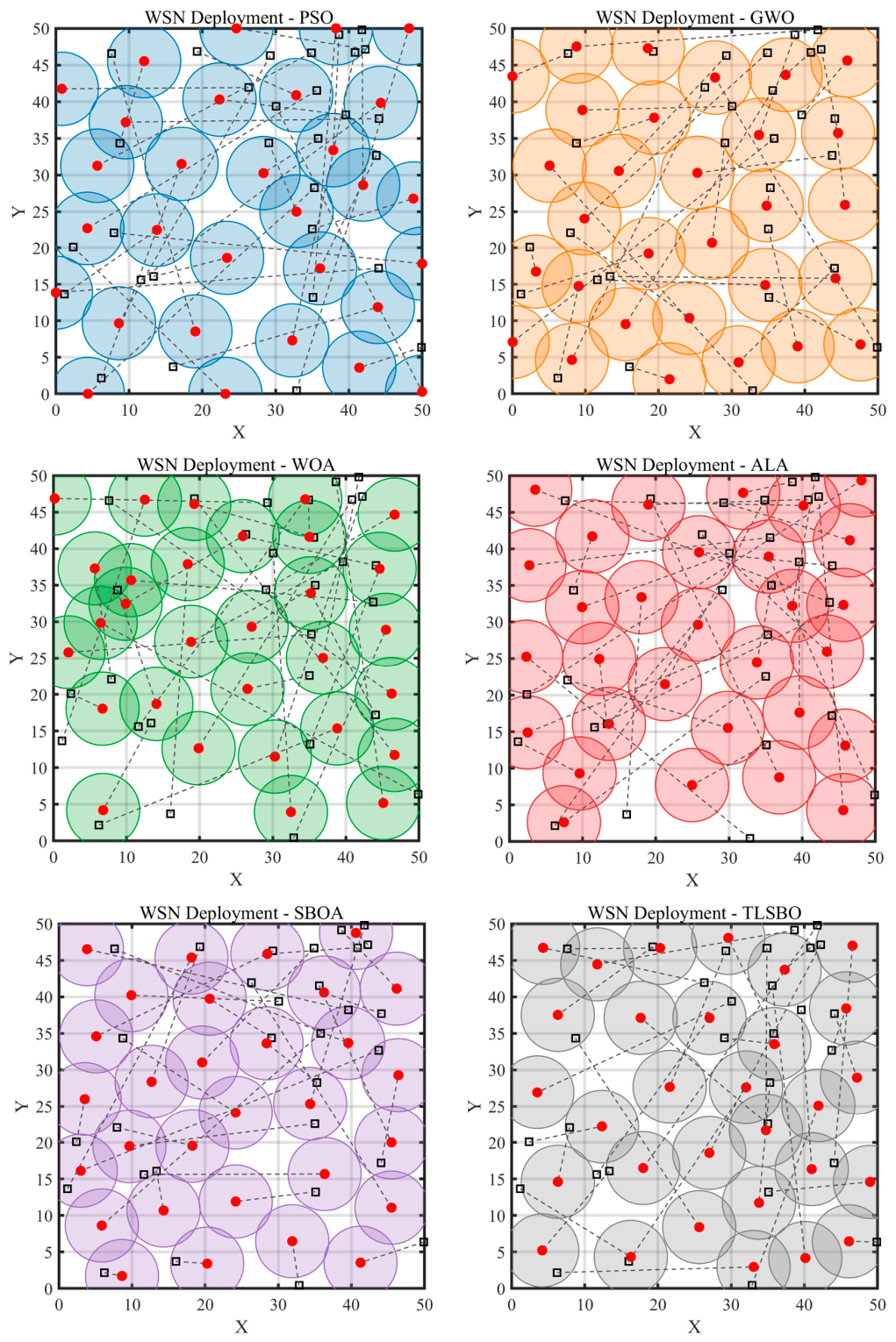
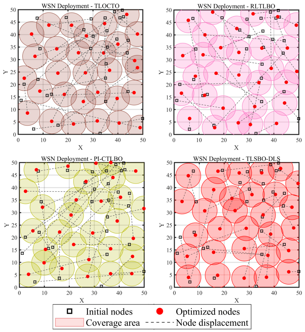
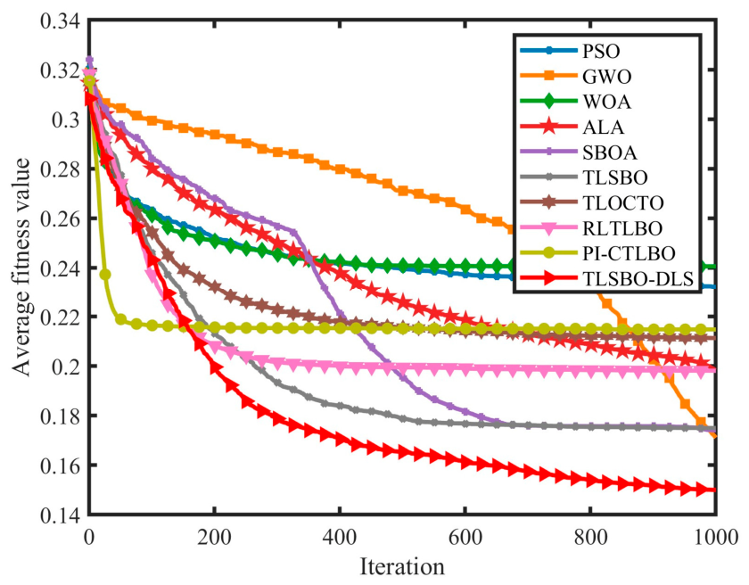
In order to assess the practical effectiveness and applicability of the proposed TLSBO-DLS algorithm in real-world engineering optimization scenarios, it is applied to the wireless sensor network (WSN) node deployment problem, which is a typical multi-objective constrained optimization task. A comprehensive comparative study is conducted against nine algorithms, including PSO, GWO, WOA, ALA, SBOA, the original TLSBO, TLOCTO, RLTLBO, and PI-CTLBO, in terms of coverage rate, redundant coverage rate, average movement distance, overall fitness, convergence characteristics, and spatial distribution of nodes. The corresponding experimental findings are illustrated in

Table 8. Statistical results of different algorithms for the WSN deployment problem ($N_d=30$).

Algorithm	Coverage	Redundancy	Move	Mean	Std	Mean Rank	Rank
PSO	0.7594	0.0737	22.9216	0.2323	0.0100	9.17	9
GWO	0.8262	0.0356	18.1726	0.1711	0.0144	2.87	2
WOA	0.7600	0.1170	22.9143	0.2406	0.0163	9.37	10
ALA	0.8173	0.0803	21.4223	0.1983	0.0119	5.70	6
SBOA	0.8357	0.0660	18.5568	0.1741	0.0130	3.00	3
TLSBO	0.8335	0.0702	18.3260	0.1750	0.0264	3.50	4
TLOCTO	0.7938	0.0968	20.9445	0.2113	0.0159	6.83	7
RLTLBO	0.8101	0.0805	20.5215	0.1981	0.0116	5.47	5
PI-CTLBO	0.7919	0.0824	22.2089	0.2148	0.0092	7.47	8
TLSBO-DLS	0.8550	0.0515	15.8471	0.1500	0.0141	1.63	1

as well as in Figure 12 and Figure 13.

As shown in Table 8, under the scenario with 30 sensor nodes, TLSBO-DLS achieves the best performance across all key evaluation metrics. In terms of coverage rate, TLSBO-DLS reaches 0.8550, outperforming traditional algorithms such as PSO, GWO, and WOA, as well as competitive algorithms such as SBOA and the original TLSBO. This indicates that TLSBO-DLS can more effectively determine node positions, reduce coverage holes, and improve overall sensing coverage.

Regarding redundant coverage rate, TLSBO-DLS achieves a value of only 0.0515, which is the lowest among all algorithms. This demonstrates that the algorithm minimizes node overlap while maintaining high coverage, thereby reducing sensing redundancy and improving energy efficiency.

In terms of average movement distance, TLSBO-DLS achieves a value of 15.8471, which is significantly lower than those of PSO, WOA, GWO, and the original TLSBO. This indicates that the algorithm can accomplish deployment optimization with lower movement cost, making it more suitable for practical scenarios with energy constraints and mobility limitations.

From the perspective of overall fitness, TLSBO-DLS attains the lowest mean value of 0.1500 among all algorithms, with a relatively low standard deviation and an average ranking of 1.63. This significantly outperforms the second-ranked GWO, the third-ranked SBOA, and the original TLSBO, demonstrating its superior accuracy and stability in multi-objective optimization.

Figure 12 illustrates the optimized node deployment layouts obtained by different algorithms, providing a visual validation of the above findings. The node distribution generated by TLSBO-DLS is more uniform, with no obvious coverage holes and minimal overlapping regions, resulting in a compact and complete coverage pattern. In contrast, algorithms such as PSO and WOA exhibit issues such as node clustering, uneven distribution, and local coverage gaps. Although GWO, SBOA, and the original TLSBO show some improvements, their deployment uniformity and coverage completeness remain inferior to those of TLSBO-DLS.

Figure 13 presents the average convergence curves of different algorithms for the WSN deployment problem, reflecting their optimization efficiency. TLSBO-DLS exhibits the fastest decline in the early stage, quickly escaping the initial random distribution and approaching high-quality solutions. During the middle stage, it maintains a steady descent without significant oscillations or premature stagnation. In the later stage, it continues to fine-tune node positions, further improving deployment quality and ultimately converging to the lowest fitness value. In contrast, PSO and WOA converge more slowly and are prone to being trapped in local optima, while GWO, SBOA, and the original TLSBO lag behind TLSBO-DLS in both convergence speed and final optimization accuracy.

Based on the quantitative results, node distribution visualizations, and convergence characteristics, it can be concluded that TLSBO-DLS achieves an optimal balance among coverage performance, resource utilization, and node movement cost in the WSN deployment problem, while also exhibiting faster convergence and stronger robustness. These results demonstrate that the proposed dimension-adaptive updating, dance learning strategy, and elite adaptive perturbation not only enhance the performance of the algorithm on benchmark functions but also provide significant advantages in complex, constrained, multi-objective real-world engineering scenarios, highlighting its strong practical value and application potential.

5. Additional Engineering Applications

To further validate the robustness and practical applicability of the proposed TLSBO-DLS algorithm, this section applies it to two classical constrained engineering optimization problems: the pressure vessel design problem and the tension/compression spring design problem. Such tasks involve nonlinear constraint conditions and are commonly adopted as standard test cases for assessing the effectiveness of optimization methods.

5.1. Pressure Vessel Design Problem

The pressure vessel design problem aims to minimize the total manufacturing cost of a cylindrical pressure vessel capped at both ends by hemispherical heads [36]. Four design variables are considered: shell thickness ($x_1$), head thickness ($x_2$), inner radius ($x_3$), and cylindrical section length ($x_4$). The corresponding mathematical model can be expressed as follows:

$${\displaystyle \genfrac{}{}{0pt}{}{\min f\left(\mathbf{x}\right)=0.6224x_1{x}_3{x}_4+1.7781x_2{x}_3^2+3.1661x_1^2{x}_4+19.84x_1^2{x}_3}{\begin{array}{c}\mathrm{s}.\mathrm{t}. g_1\left(\mathbf{x}\right)=-x_1+0.0193x_3\le 0\\ g_2\left(\mathbf{x}\right)=-x_2+0.00954x_3\le 0\\ g_3\left(\mathbf{x}\right)=-\pi x_3^2{x}_4-\frac{4}{3}\pi x_3^3+1296000\le 0\\ g_4\left(\mathbf{x}\right)=x_4-240\le 0\\ 0.0625\le x_1,x_2\le 6.1875, 10\le x_3,x_4\le 200\end{array}}}$$

(32)

Table 9. Statistical results obtained by different algorithms for the pressure vessel design problem.

Algorithm	Best	Mean	Std	Friedman Rank	Rank
PSO	5.90751E+03	6.25702E+03	3.07711E+02	8.87	9
GWO	5.88709E+03	6.04860E+03	3.60216E+02	7.83	8
WOA	6.16368E+03	8.09252E+03	1.15336E+03	9.93	10
ALA	5.88533E+03	5.88551E+03	3.41009E−01	3.40	2
SBOA	5.88533E+03	5.91495E+03	6.44248E+01	6.40	7
TLSBO	5.88533E+03	5.88597E+03	1.80186E+00	3.87	5
TLOCTO	5.88533E+03	5.88551E+03	3.02130E−01	3.73	4
RLTLBO	5.88533E+03	5.88585E+03	9.82698E−01	3.63	3
PI-CTLBO	5.88534E+03	5.91418E+03	1.11402E+02	4.37	6
TLSBO-DLS	5.88533E+03	5.88551E+03	3.41009E−01	2.97	1

presents the comparison results of different algorithms on the pressure vessel design problem.

From the statistical results presented in Table 9, TLSBO-DLS demonstrates a significant performance advantage in the pressure vessel design problem. In terms of the best solution (Best), TLSBO-DLS achieves 5.88533 × 10³, which is identical to the results obtained by ALA, SBOA, TLSBO, TLOCTO, and RLTLBO, and outperforms PSO (5.90751 × 10³), GWO (5.88709 × 10³), WOA (6.16368 × 10³), and PI-CTLBO (5.88534 × 10³).

Regarding the mean value (Mean), TLSBO-DLS attains 5.88551 × 10³, which is equal to ALA and TLOCTO, and significantly lower than PSO (6.25702 × 10³), GWO (6.04860 × 10³), WOA (8.09252 × 10³), SBOA (5.91495 × 10³), TLSBO (5.88597 × 10³), RLTLBO (5.88585 × 10³), and PI-CTLBO (5.91418 × 10³).

In terms of standard deviation (Std), TLSBO-DLS records 3.41009 × 10⁻¹, which is also the lowest value together with ALA and TLOCTO, and is substantially smaller than PSO (3.07711 × 10²), GWO (3.60216 × 10²), WOA (1.15336 × 10³), SBOA (6.44248 × 10¹), TLSBO (1.80186 × 10⁰), RLTLBO (9.82698 × 10⁻¹), and PI-CTLBO (1.11402 × 10²), indicating superior stability.

According to the Friedman ranking, TLSBO-DLS ranks first with a score of 2.97, followed by ALA (3.40), RLTLBO (3.63), TLOCTO (3.73), and the original TLSBO (3.87).

These results demonstrate that TLSBO-DLS outperforms the compared algorithms in terms of solution accuracy, convergence stability, and overall performance, making it a highly effective and reliable approach for solving constrained engineering optimization problems such as pressure vessel design.

5.2. Tension/Compression Spring Design Problem

This optimization case aims to reduce the mass of a tension/compression spring while satisfying limitations related to shear stress, natural frequency, and deformation. The decision variables consist of wire diameter ($x_1$), mean coil diameter ($x_2$), and number of active coils ($x_3$):

$${\displaystyle \genfrac{}{}{0pt}{}{\min f\left(\mathbf{x}\right)=(x_3+2)x_2{x}_1^2}{\begin{array}{c}\mathrm{s}.\mathrm{t}. g_1(\mathbf{x})=1-\frac{x_2^3{x}_3}{71785x_1^4}\le 0\\ g_2(\mathbf{x})=\frac{4x_2^2-x_1{x}_2}{12566(x_2{x}_1^3-x_1^4)}+\frac{1}{5108x_1^2}-1\le 0\\ g_3(\mathbf{x})=1-\frac{140.45x_1}{x_2^2{x}_3}\le 0\\ g_4(\mathbf{x})=\frac{x_1+x_2}{1.5}-1\le 0\\ 0.05\le x_1\le 2.0, 0.25\le x_2\le 1.3, 2\le x_3\le 15\end{array}}}$$

(33)

Table 10. Statistical results obtained by different algorithms for the tension/compression spring design problem.

Algorithm	Best	Mean	Std	Friedman Rank	Rank
PSO	1.26655E−02	1.34359E−02	9.66023E−04	8.13	9
GWO	1.26792E−02	1.27433E−02	6.16092E−05	8.03	8
WOA	1.26655E−02	1.38379E−02	1.20376E−03	9.23	10
ALA	1.26652E−02	1.26777E−02	3.12293E−05	3.13	2
SBOA	1.26653E−02	1.26791E−02	1.90616E−05	4.10	3
TLSBO	1.26654E−02	1.26849E−02	1.33300E−05	5.60	7
TLOCTO	1.26656E−02	1.26766E−02	8.56222E−06	4.47	5
RLTLBO	1.26653E−02	1.26755E−02	1.11549E−05	4.13	4
PI-CTLBO	1.26652E−02	1.26894E−02	2.18705E−05	5.20	6
TLSBO-DLS	1.26656E−02	1.26697E−02	3.82459E−06	2.97	1

presents the best (Best), mean (Mean), standard deviation (Std), and Friedman ranking results of TLSBO-DLS compared with other algorithms.

In terms of the best value (Best), TLSBO-DLS achieves 1.26656 × 10⁻², which is very close to ALA (1.26652 × 10⁻²), SBOA (1.26653 × 10⁻²), RLTLBO (1.26653 × 10⁻²), and PI-CTLBO (1.26652 × 10⁻²), placing it within the optimal range and clearly outperforming PSO, GWO, WOA, the original TLSBO, and TLOCTO.

Regarding the mean value (Mean), TLSBO-DLS attains 1.26697 × 10⁻², which is the lowest among all compared algorithms, significantly better than ALA (1.26777 × 10⁻²), SBOA (1.26791 × 10⁻²), TLSBO (1.26849 × 10⁻²), TLOCTO (1.26766 × 10⁻²), RLTLBO (1.26755 × 10⁻²), PI-CTLBO (1.26894 × 10⁻²), as well as PSO, GWO, and WOA.

In terms of standard deviation (Std), TLSBO-DLS records 3.82459 × 10⁻⁶, which is substantially smaller than that of almost all other algorithms, being only slightly higher than TLOCTO, thereby demonstrating excellent stability and robustness.

According to the Friedman ranking, TLSBO-DLS ranks first with a score of 2.97, followed by ALA (3.13), SBOA (4.10), RLTLBO (4.13), and TLOCTO (4.47).

These results indicate that TLSBO-DLS achieves superior convergence accuracy, stability, and overall optimization capability in the spring design problem, and is able to solve such constrained engineering optimization tasks in a stable and efficient manner.

In summary, the multi-strategy enhancement mechanism proposed in TLSBO-DLS not only demonstrates excellent performance on the CEC benchmark functions but also exhibits superior optimization accuracy, convergence stability, and practical applicability in constrained and highly nonlinear real-world engineering optimization problems.

6. Conclusions and Future Work

This study focuses on overcoming the shortcomings of the TLSBO algorithm when dealing with high-dimensional and complex optimization tasks, including insufficient search capability, susceptibility to local optima, and poor convergence stability, by proposing a multi-strategy enhanced algorithm, namely TLSBO-DLS. By incorporating a dimension-adaptive update probability strategy, a dance learning strategy, and an elite adaptive perturbation mechanism, the proposed algorithm enables a more efficient trade-off between broad search capability and refined local optimization. The results obtained from experiments conducted on the CEC2017, CEC2020, and CEC2022 benchmark sets indicate that TLSBO-DLS exhibits superior performance compared to a range of advanced optimization algorithms, particularly in terms of solution quality, convergence efficiency, and stability. Furthermore, in the wireless sensor network node deployment model constructed in this study, the proposed algorithm effectively improves coverage, reduces redundant coverage, and minimizes node movement cost, thereby validating its practical applicability in real-world engineering problems.

Despite the promising performance achieved, several limitations remain. First, the integration of multiple strategies increases the algorithmic complexity, which may introduce additional computational overhead. Second, some parameters of the algorithm (e.g., weighting coefficients and strategy activation probabilities) are still determined empirically, and their adaptability requires further improvement. In addition, the current study mainly focuses on a single-objective optimization framework, while the capability of handling multi-objective optimization problems has not been fully explored.

Subsequent research will be directed toward several key avenues. To begin with, efforts will be made to design more self-regulating parameter adjustment strategies, thereby decreasing the dependence on manual configuration. In addition, the algorithm is expected to be further developed to handle both multi-objective scenarios and dynamically changing optimization environments. Another important direction involves incorporating techniques from machine learning and reinforcement learning to improve its adaptability when facing complex and uncertain conditions. Moreover, the applicability of the method will be explored across a broader spectrum of engineering problems, including three-dimensional wireless sensor network deployment, path optimization, and intelligent scheduling, in order to comprehensively assess its versatility and practical significance.