Research on Eddy Currents in Dry Cool Superconducting MRI Systems Based on Multi-Physics Field Coupling Analysis

Abstract

This study investigates eddy currents in the dry cool superconducting MRI system by adopting a strong coupling multi-physics analysis method that integrates electromagnetic and mechanical fields. The 3D model is simplified based on the spatial distribution characteristics of the Lorentz force. A set of strong coupling matrix equations is derived by combining mechanical principles with Maxwell’s equations. The weak coupling scheme is implemented by applying displacement boundary conditions and validated through kinetic energy analysis. Through vector analysis, the origin of eddy power is explored, leading to the conclusion that the primary contribution to eddy power stems from the coupling between primary and secondary eddy currents. Furthermore, by analyzing the vector directions of primary and secondary eddy currents at specific mesh elements, the sign (positive or negative) of eddy power at different frequencies is characterized. The results show that the superposition of primary and secondary eddy currents produces positive power when they have a common directional component; conversely, the suppressive effect of secondary eddy currents results in negative power. This research deepens the understanding of the generation mechanism and influence of secondary eddy currents, providing guidance for subsequent dry cool superconducting MRI magnet optimization design.

1. Introduction

Unlike traditional liquid helium cooled magnets, dry cool superconducting magnets feature a compact structure, low maintenance costs, and convenient operation, which have become a mainstream development direction for modern MRI systems. Dry cool superconducting MRI magnets operate without liquid helium and adopt a vacuum environment instead. When superconducting coils generate heat due to eddy currents, the heat cannot be removed by liquid helium. Alternatively, heat is dissipated through thermal conduction via thermal bus structures. Therefore, it is of great necessity and engineering significance to systematically investigate the eddy current characteristics and suppression methods for dry cool superconducting MRI magnets.

In dry cool superconducting MRI systems, gradient coils are typically placed inside the magnet, surrounded by various types of conductive structures. These include the pole plates and iron yoke structures of permanent magnets, the cryostat structure of superconducting magnets (comprising vacuum vessels, liquid helium vessels, and thermal shields), the framework of superconducting magnets, radio frequency shields, room-temperature shim coils, and more [1]. In MRI scanning, gradient coils must be rapidly switched on and off in coordination with radio frequency pulses according to the imaging pulse sequence. This process enables the spatial localization of nuclear magnetic resonance (NMR) signals and allows for the measurement of tissue parameters in the examined subject. Typically, gradient current pulses take the form of trapezoidal waveforms. The magnet investigated in this study employs an active shielding method to reduce the alternating gradient fields generated by the gradient coils (GCs). This is achieved by designing shielding coils placed outside the gradient coils, through which a reverse current is passed to reduce the magnetic field beyond the shielding coils. However, the magnetic field cannot be completely eliminated, and stray fields still exist, which induce eddy currents in the thermal shield according to Faraday’s law of electromagnetic induction [2]. These eddy currents usually exhibit complex spatial and temporal distributions.

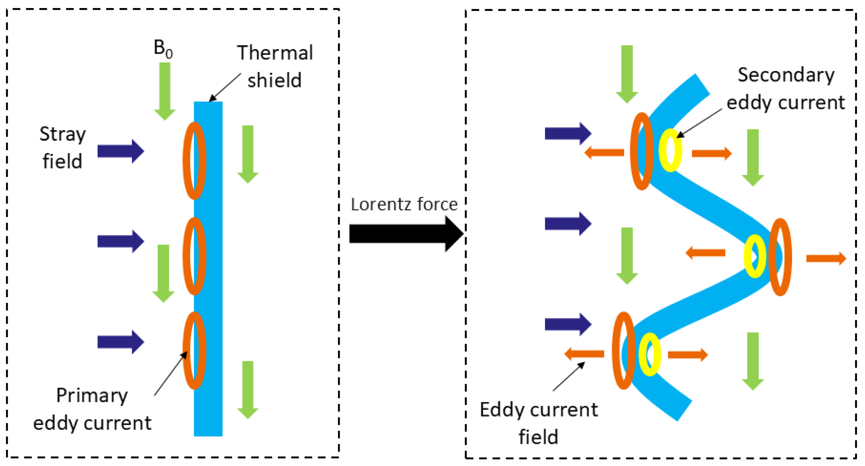
According to Lenz’s law, the temporal variation in the induced eddy currents opposes the current in the GC. These eddy currents can, in turn, adversely affect the MRI system and image quality in several ways. The eddy power generated by eddy currents may cause the magnetic circuit temperature to deviate from its ideal operating state, alter the operating temperature of the magnet, and in extreme cases, may even trigger a magnet quench [3,4]. Under the influence of the static magnetic field, the eddy currents within the conductors are subjected to Lorentz forces, causing vibrations in other components of the MRI system. This vibration radiates noise externally, thereby reducing patient comfort and deteriorating image quality [5,6,7]. In addition, it may generate oscillatory currents within the system [8,9]. Furthermore, the vibration of the thermal shield induced by Lorentz forces cuts the magnetic flux lines of the main magnetic field, generating secondary eddy currents. These secondary eddy currents interact with the primary eddy currents and subsequently transmit magnetic fields to the superconducting main coil, causing it to heat up and potentially leading to a quench. This process is illustrated in Figure 1. The left dashed box illustrates the formation process of the primary eddy current. Under the action of the Lorentz force, the secondary eddy current shown in the right dashed box is generated. In this figure, $B_0$ refers to the main magnetic field produced by the superconducting coil when energized with direct current, acting as the background field for the generation of eddy currents.

Not only that, but according to Lenz’s law, eddy currents cause distortion in the magnetic field pulse waveform, leading to a reduction in the switching speed of gradient pulses of GC. This consequently limits the application of fast and ultra-fast imaging pulse sequences. The magnetic field generated by secondary eddy currents in the imaging region superimposes onto the magnetic field produced by the GC, degrading the spatiotemporal characteristics of the gradient magnetic field. This results in erroneous localization of NMR signals and causes distortion in MRI images [9,10]. These geometric distortions include shear deformation caused by readout eddy current gradients, stretch deformation caused by phase-encoding eddy current gradients, and image displacement caused by ${\mathit{B}}_0$ eddy currents [11,12,13]. In diffusion imaging or Echo Planar Imaging (EPI), these geometric distortions become even more severe [13]. Additionally, eddy currents can lead to intensity-phase variations in images and spectra [14]. To mitigate the adverse effects of eddy currents on MRI equipment and image quality, researchers have proposed a series of solutions. Methods such as lamination techniques [15,16] and the insertion of thermal shield conductors [17,18] can reduce eddy currents to some extent. However, secondary eddy currents still persist. To address the issue of unwanted transient magnetic fields induced by eddy currents in conductive shielded rooms due to the rapid turn-off of polarization coil currents in ultra-low field MRI, ref. [19] proposed two physical models of the shielded room based on the relative position of the polarization coil and the shielded room to simulate the transient fields, and verified the consistency between simulation and experimental results, which provides guidance for the structural design of conductive shielded rooms and the development of eddy current cancellation techniques. Ref. [20] developed and validated the TVEDDY algorithm, a retrospective three-parameter exponential decay model, to characterize and correct time-varying eddy current artifacts in oscillating gradient spin-echo (OGSE) diffusion MRI, demonstrating its superior performance over conventional correction methods in reducing artifacts and improving image quality for gradient-intensive diffusion acquisitions. In 2021, ref. [21] conducted finite element analysis using Opera-3D software to investigate quench-induced eddy currents and the resulting mechanical stresses/deformations in the bobbin structure and thermal shield of a 1.5 T superconducting MRI magnet system, comparing the effects on different metallic alloys to provide design inputs for these components. In 2023, ref. [22] tailored the Multi-layer Integral Method (TMIM) for general eddy current analysis in thin structures, comparing it with the network-analysis (NA) method and Ansys Maxwell simulations to analyze z-gradient eddy currents, validate passive shielding configurations, and demonstrate effective pre-emphasis compensation for eddy current mitigation in MRI systems. In the same year, ref. [23] presented a novel computational approach that leverages high-resolution electromagnetic simulations and frequency-domain superposition to optimize gradient array performance, minimizing eddy power losses within the cryostat while preserving key MRI system parameters such as field linearity and gradient strength. In 2024, ref. [24] present a systematic method, based on time-domain Maxwell’s equations, to calculate spatially resolved eddy current heating power density in thin conductive objects exposed to time-varying magnetic fields from multiple independent coils, validated against experimental temperature rise measurements in an MRI scanner, which enables accurate prediction and mitigation of gradient-induced conductor heating in MRI and related instruments. In the same year, ref. [25] developed a theoretical framework and mitigation strategy for motional eddy currents in high-field MRI eddy current shielding, demonstrating that patterned copper shields can suppress vibration-induced currents and improve shielding performance in high-static magnetic field environments. In 2025, ref. [26] proposed an efficient finite element analysis framework to characterize eddy current effects from z-gradient coils in low-field MRI, introducing an equivalent system model to reduce computational complexity and deriving the gradient eddy-current impulse response function (GEIRF) to guide pre-emphasis design, validated through experiments on a 50 mT portable MRI system. In summary, numerous scholars have continuously investigated the eddy currents generated by gradient coils in MRI in recent years, and various methods have been adopted to reduce or eliminate eddy currents. Therefore, it is essential to further explore the generation mechanism and evolution process of eddy currents.

It is evident that the eddy current issue in superconducting MRI systems constitutes a complex electromagnetic–mechanical multi-physics coupling process. Many researchers have employed multi-physics coupling solution methods to perform high-precision calculations of eddy currents in MRI systems. Based on the principles of decoupling, multi-physics coupling solution methods can be categorized into weak coupling and strong coupling. Among these, weak coupling is also referred to as loose coupling or sequential coupling, while strong coupling is known as full coupling or direct coupling [27].

Weak coupling involves the iterative analysis of two or more physical fields in a specific sequence, where the calculation results from one physical process are transferred as loads to another. This approach is effective for solving multi-physics coupling problems, where it is difficult to establish degrees of freedom that encompass all coupling physical fields and where nonlinearity is not highly pronounced. Employing weak coupling methods for such problems can reduce the dimensionality of the analytical model, alleviate ill-conditioning in system equations, and lower computational costs [28]. Typical applications of weak coupling include thermal stress analysis [29], induction heating analysis, steady-state fluid–structure interaction [30,31], electrostatic-structural coupling, and electric current conduction—magnetostatic coupling. For instance, in the static structural coupling analysis of micro electromechanical system switches [32], electric field analysis and stress-strain analysis are performed alternately. The advantages of the weak coupling method lie in its ease of implementation, high computational efficiency, and the ability to fully leverage existing mature commercial simulation software, making it widely applicable. However, compared to strong coupling, weak coupling tends to be less accurate in computation. When solving multi-physics coupling problems using weak coupling, each physical field is analyzed sequentially, with the results from the previous analysis applied as loads to the subsequent one. The iteration ends once the coupled state variables converge. In contrast, the strong coupling method simultaneously establishes and solves the governing equations for all physical fields by incorporating the degrees of freedom from all coupling fields at once.

A typical application of strong coupling is thermoelectric analysis. For instance, researchers have used the finite element method and strong coupling heat transfer theory to transform the external boundary conditions between components into internal boundary conditions within the components. This approach allows for direct coupled simulation of the components, determines boundary conditions through empirical formulas, and acquires initial heat transfer conditions by simulating operational processes. This significantly simplifies boundary conditions and enhances the rationality of the heat transfer analysis process [33]. The strong coupling method typically requires the use of coupled field elements that encompass all necessary degrees of freedom. Decoupling is achieved by solving the coupled element matrices or load vectors, enabling a more accurate determination of the unknown variables for each physical field.

Dry cool superconducting MRI, as a crucial medical imaging tool, is now widely used in clinical diagnosis and scientific research. As the application scope of MRI technology continues to expand and innovate, higher demands are placed on the imaging quality of MRI equipment and the reliability of superconducting magnets. Against this backdrop, this paper investigates the eddy currents in a dry cool superconducting MRI system. This study focuses on the electromagnetic–mechanical multi-physics coupling problem, conducting analyzes through strong coupling and weak coupling approaches. Simulations are performed, and the results are analyzed. An in-depth examination of the generation processes and mechanisms of eddy currents in the system is provided, offering guidance for the subsequent optimization design of the magnet and gradient coils.

2. Theoretical Model and Numerical Methods

2.1. Theoretical Model

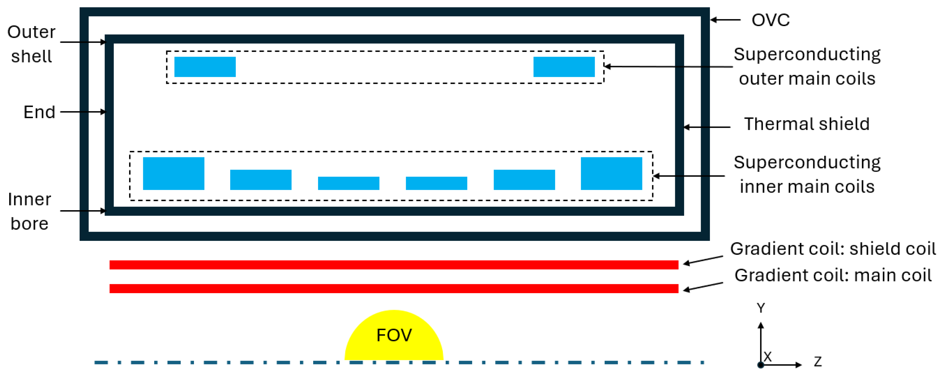
Figure 2 shows a cross-sectional schematic diagram of the dry cool superconducting MRI system and its GC. The cryostat of the superconducting magnet contains two cylindrical conductive structures: the Outer Vacuum Chamber (OVC) at room temperature and the thermal shield at 50 K. The GC is located within the inner bore of the magnet and consists of two parts: the main coil and the shield coil. The main function of the shield coil is to reduce the stray field outside the gradient coil, thereby minimizing eddy currents in the magnet. FOV refers to the field of view of the MRI system, which is adopted to schematically illustrate the operating principle of the MRI system.

The dimensions of the model shown in the above figure are listed in the table below, and the dimensions of the 3D model used in the subsequent text are consistent with those in the table.

The OVC at room temperature is made of stainless steel, while the thermal shield at 50 K is constructed from high-purity aluminum, leveraging its extremely high electrical conductivity at low temperatures to shield against the stray field generated by GC. To facilitate simulation and computation, the superconducting coils were assumed to be copper-based materials, and inter-turn interactions were neglected. Regarding GC, due to the complex structure of the transverse coils, where the coil cross-section is only on the millimeter scale, it would increase mesh complexity, leading to higher computational costs and longer processing times. Therefore, in this study, a finite element model was not established for GC. Instead, it was treated as a series of short straight current segments. In this approach, the tiny cross-section of the gradient coil was ignored, and only the magnetic field generated inside the OVC of the magnet was considered. According to Equation (1), the magnetic field produced by each short straight current segment can be calculated using the Biot–Savart law, followed by a line integral.

$$\mathit{B}\left(\mathit{r}\right)=\frac{1}{4\pi \nu }{\int }_C\frac{I\mathit{dl}\times {\mathit{r}}^{\prime }}{|{\mathit{r}}^{\prime }{|}^3}$$

(1)

where I is the current amplitude within the line source and $\mathit{dl}$ is its differential, and $\nu$ represents the magnetic reluctivity.

2.2. Numerical Methods

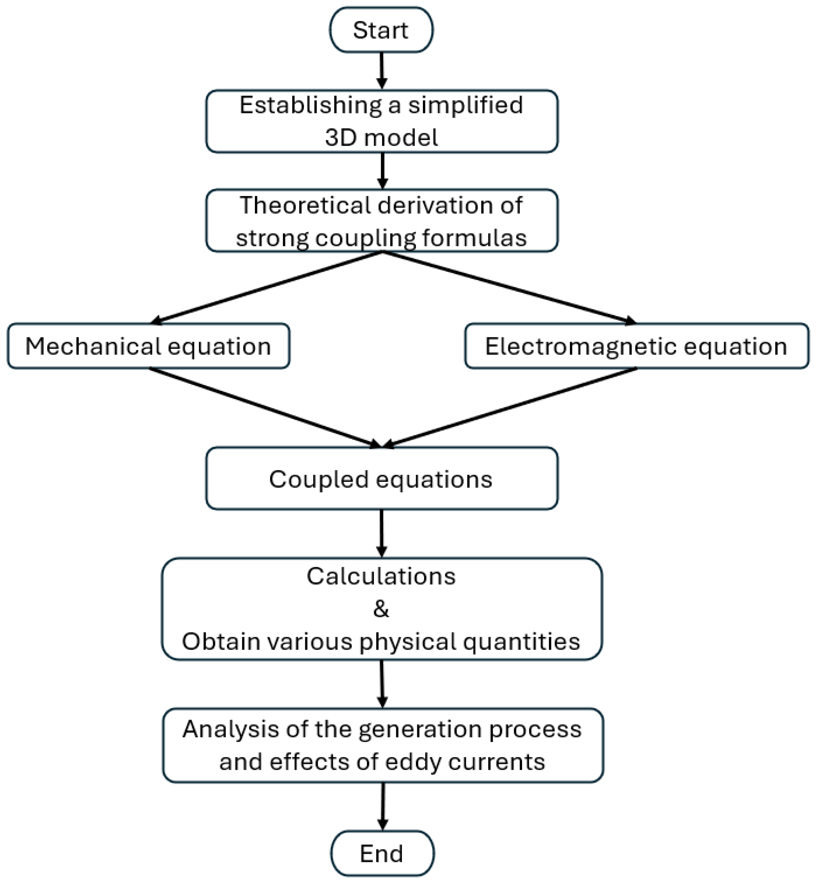
This study focuses on eddy currents in a dry cool superconducting MRI system. Addressing the coupled electromagnetic–mechanical multi-physics problem, it conducts a strong coupling analysis and a weak coupling analysis, followed by simulation calculations. Based on the computational results, the generation processes of primary and secondary eddy currents, as well as the relationship between them, were analyzed by examining the magnetic field distribution, eddy currents, eddy current power, and kinetic energy in various parts. The influence of eddy currents on the dry cool superconducting magnet is revealed through the eddy power distribution on the thermal shield, providing guidance for the subsequent optimization design of the magnet and GC. The specific research methodology and process are illustrated in Figure 3.

The specific details are as follows:

• During the model establishment stage, a 3D model is created based on the structural diagram shown in Figure 2, excluding the GC. Since this study focuses on eddy currents generated by the transverse GC, an axisymmetric model cannot be used. Meanwhile, the X-GC and Y-GC have identical structures, differing only by a 90-degree spatial rotation; therefore, this paper selects only the Y-GC for investigation. It is important to note that the Lorentz forces acting on the metal components are not symmetric in all directions, thus requiring discussion. This analysis helps determine the symmetry of the magnet, facilitating the simplification of the 3D model and reducing computational time.
• During the theoretical derivation stage of strong coupling, the mechanical equation employed Navier’s equation of motion, while the electromagnetic equation is derived from Maxwell’s equations. Vector analysis was performed separately for each. Coupling equations were established based on the coupled physical quantities. Minor and high-order terms were neglected or simplified, resulting in a system of strong coupling matrix equations in the frequency domain.
• In the results comparison stage, based on the computational outcomes from both strong coupling and weak coupling methods, various parameters of thermal shield components—such as eddy currents, eddy power, and kinetic energy are compared. The results from the two coupling methods were subtracted to isolate the effects attributable solely to secondary eddy currents. These were then compared with the results from the weak coupling simulation, which only reflect the effects of primary eddy currents, thereby illustrating the relationship between primary and secondary eddy currents.
• Finally, based on the above calculations and analysis results, recommendations were provided regarding the optimized design direction for the dry cool superconducting MRI system to address eddy current issues.

3. Simplified 3D Model and Coupling Formulas

3.1. Simplified 3D Model

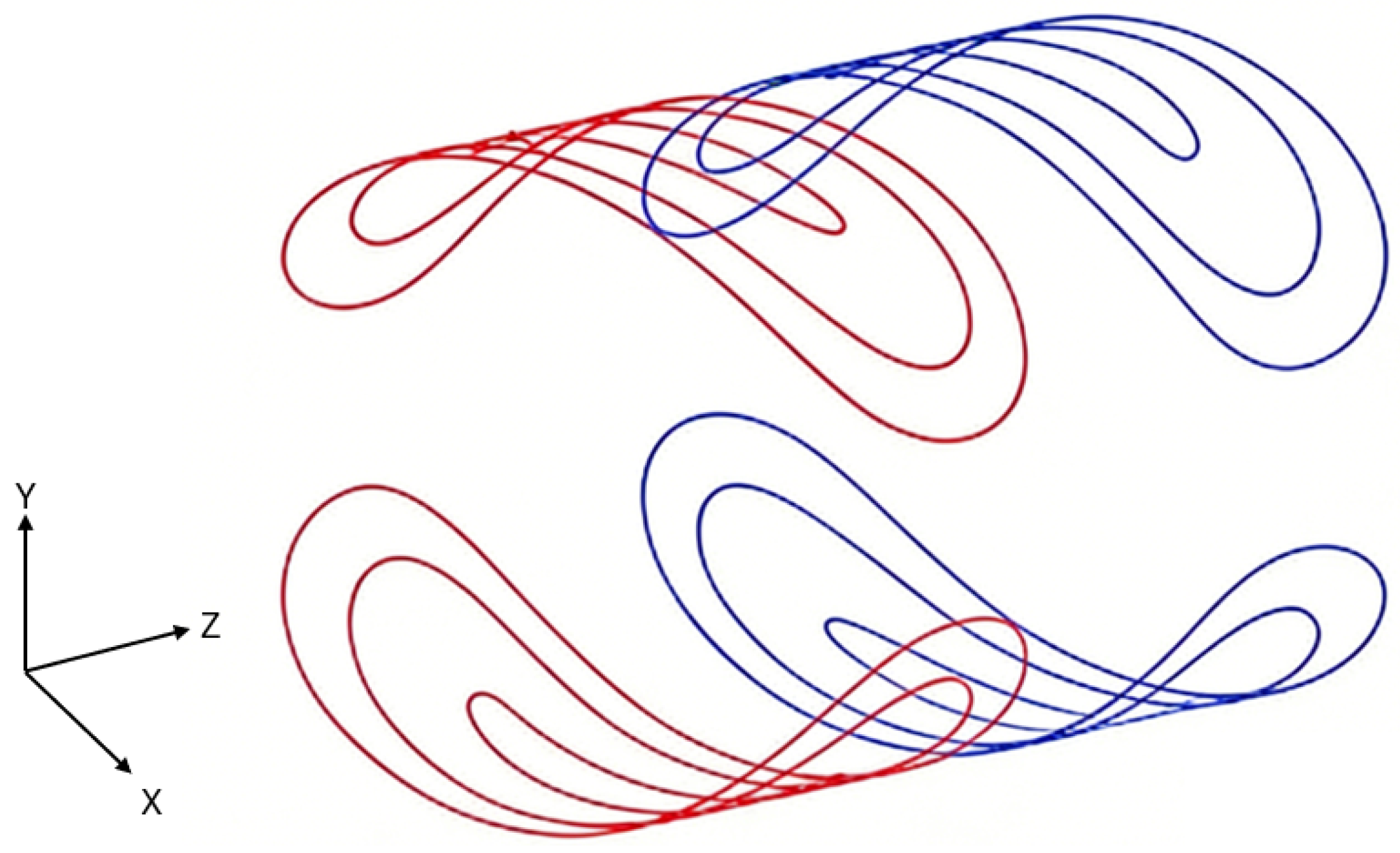
To improve simulation efficiency, the 3D model needs to be simplified using symmetry to avoid building a complete cylindrical magnet model. Based on the aforementioned simplification of GC, each turn of the gradient coil can be considered independent and unconnected. According to the Biot–Savart law in Equation (1), each coil generates a magnetic field from the input current. The structure of the Y-GC at this point is shown in Figure 4. It shows the schematic diagram of the Y-direction gradient coil adopted in this study, which is a simplified representation of the actual engineering product. It exhibits geometric symmetry with respect to the X-Y plane, the Y-Z plane, and the X-Z plane. Therefore, the degree of simplification of the magnet needs further discussion based on the symmetry of the Lorentz force components acting on the magnet in various directions.

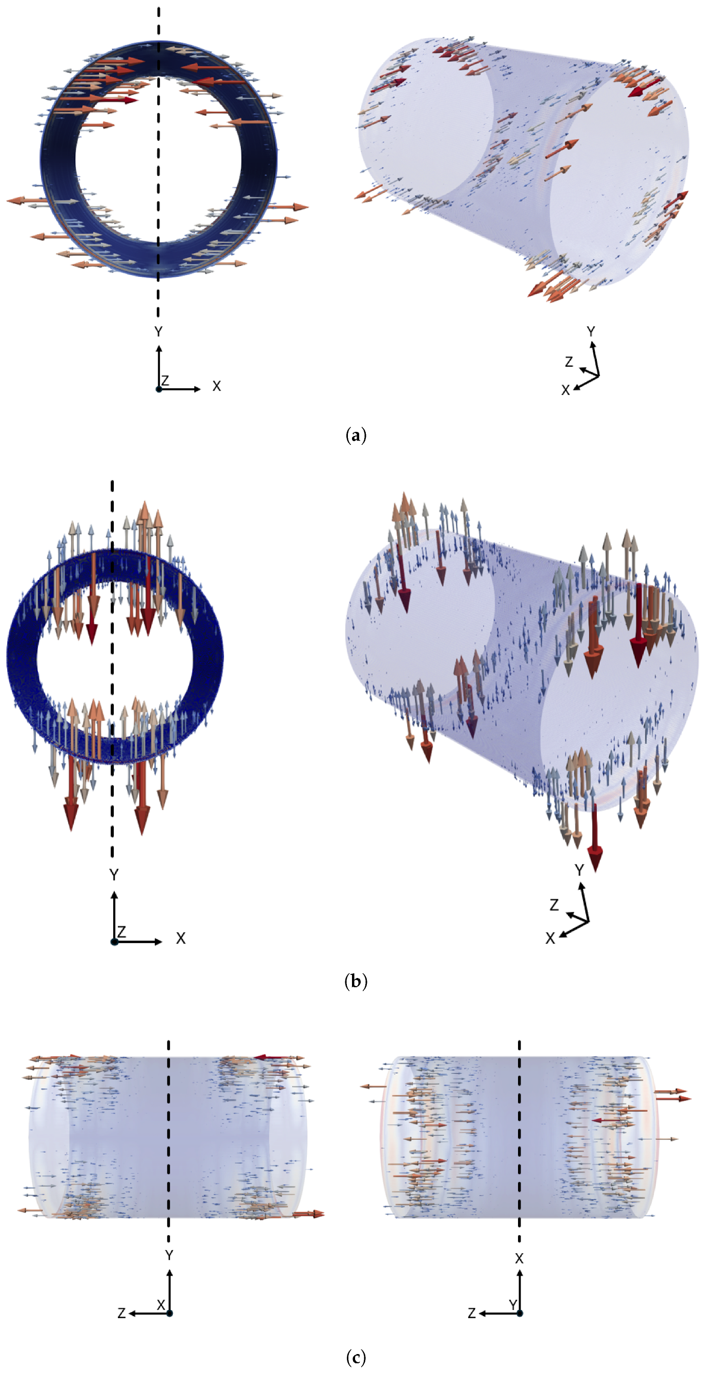
Taking the inner bore of the high-conductivity thermal shield as an example, when an alternating current is applied to GC, according to Faraday’s law of electromagnetic induction, eddy currents are induced in the conductor, and these currents are subjected to electromagnetic forces under the influence of the magnetic field. Figure 5 presents the simplified model of the inner bore of the thermal shield, where a cylindrical structure is used to equivalent the practical configuration. When the Y-GC is energized with an alternating current of a specific frequency, the schematic diagram of Lorentz force components in all directions of the thermal shield from different perspectives is shown in Figure 5a–c.

From Figure 5a,b, it can be observed that the X-component and Y-component of the Lorentz force acting on the inner bore of the thermal shield are symmetric with respect to the Y-Z plane. Therefore, the complete cylindrical magnet model can be simplified to a half model symmetric about the Y-Z plane. Furthermore, from Figure 5c, it can be seen that the Z-component of the Lorentz force is symmetric with respect to the X-Y plane. Hence, the magnet model can be further simplified to a quarter model symmetric about the X-Y plane. However, it is also noticeable that none of the components of the Lorentz force are symmetric with respect to the X-Z plane; instead, they point in the same direction on both sides of the X-Z plane. Consequently, the magnet model cannot be further simplified symmetrically and must be solved with a quarter model. Meanwhile, symmetric excitation currents are imposed on the gradient coils in accordance with the structural layout, which yields a symmetric magnetic field distribution. Furthermore, the magnetic field is properly constrained by boundary conditions. Consequently, model simplification can be reasonably implemented based on the inherent symmetry of the aforementioned Lorentz force.

3.2. Strong Coupling Formulas

3.2.1. Mechanical Equation

For the analysis of the mechanical field, since the thermal shield vibrates due to the Lorentz force in the magnetic field, it is described using Navier’s equation of motion, as shown in Equation (2).

$${\rho }_m\ddot{\mathit{u}}={\mathit{f}}_{\mathrm{ext}}+{\widehat{\mathcal{D}}}^{\mathrm{T}}\widehat{\mathit{\sigma }}$$

(2)

Here, ${\rho }_m$ is the material density of the object, and $\mathit{u}$ describes the displacement of the object. The mechanical stress tensor $\widehat{\mathit{\sigma }}$ can be simplified into a vector based on its symmetry using Voigt notation, as shown in Equation (3).

$$\mathit{\sigma }={\left(\begin{array}{cccccc}{\sigma }_{xx}& {\sigma }_{yy}& {\sigma }_{zz}& {\sigma }_{yz}& {\sigma }_{xz}& {\sigma }_{xy}\end{array}\right)}^{\mathrm{T}}$$

(3)

The differential operator $\widehat{\mathcal{D}}$ can be obtained by expanding the divergence term:

$$\widehat{\mathcal{D}}={\left(\begin{array}{ccccccc}\frac{\partial }{\partial x}& 0& 0& 0& 0& \frac{\partial }{\partial z}& \frac{\partial }{\partial y}\\ 0& \frac{\partial }{\partial y}& 0& \frac{\partial }{\partial z}& 0& 0& \frac{\partial }{\partial x}\\ 0& 0& \frac{\partial }{\partial z}& \frac{\partial }{\partial y}& \frac{\partial }{\partial x}& 0& 0\end{array}\right)}^{\mathrm{T}}$$

(4)

For small displacements, the mechanical stress $\widehat{\mathit{\sigma }}$ and strain $\widehat{\mathit{S}}$ can be treated in a linear relationship, which allows conversion via the tensor of elasticity moduli $\widehat{\mathit{c}}$.

$$\widehat{\mathit{\sigma }}=\widehat{\mathit{c}}\widehat{\mathit{S}}$$

(5)

Combined with Equation (2) and describing $\widehat{\mathit{S}}\to \mathit{S}$ using Voigt notation as $\widehat{\mathcal{D}}\mathit{u}$, this yields the following equation of motion.

$${\rho }_m\ddot{\mathit{u}}={\mathit{f}}_{\mathrm{ext}}+{\widehat{\mathcal{D}}}^{\mathrm{T}}\widehat{\mathit{c}}\widehat{\mathcal{D}}\mathit{u}$$

(6)

For the movement of the thermal shield, a velocity proportional damping term $\widehat{\mathit{R}}$, typically describing friction within the material, is also considered.

$${\rho }_m\ddot{\mathit{u}}={\mathit{f}}_{\mathrm{ext}}+{\widehat{\mathcal{D}}}^{\mathrm{T}}\widehat{\mathit{c}}\widehat{\mathcal{D}}\mathit{u}-\mathit{R}\dot{\mathit{u}}$$

(7)

3.2.2. Electromagnetic Equation

For the magnetic part Maxwell equations are used [2]:

$$\nabla ·\mathit{B}=0$$

(8)

$$\nabla ·\mathit{E}=0$$

(9)

$$\nabla \times \mathit{E}=-\frac{\partial \mathit{B}}{\partial t}$$

(10)

$$\nabla \times \nu \mathit{B}=\mathit{J}$$

(11)

Here, $\mathit{E}$, $\mathit{J}$, and $\nu$ represent the electric field intensity, current density, and magnetic reluctivity, respectively. As this study addresses a pure eddy current problem, $\mathit{E}$ is represented by a solenoidal vector field, and displacement currents are neglected. According to Equations (9) and (10), the following can be derived:

$$\frac{\partial }{\partial t}\mathit{A}=-\mathit{E}$$

(12)

Here, the magnetic vector potential $\mathit{A}$ is defined by $\mathit{B}=\nabla \times \mathit{A}$, and the Coulomb gauge is introduced as shown in Equation (13).

$$\nabla ·\mathit{A}=0$$

(13)

3.2.3. Coupled Equations

In the electromagnetic–mechanical coupling process, the magnetic field influences the structural displacement $\mathit{u}$ and velocity $\dot{\mathit{u}}$ through the electromagnetic force density ${\mathit{f}}_L$. Conversely, the velocity of the structural motion $\dot{\mathit{u}}$ affects the magnetic field distribution through the motional electromotive force. Therefore, the Lorentz force density ${\mathit{f}}_L$ serves as a coupling quantity in the numerical description of the electromagnetic–mechanical coupling process. It must be considered the exciting force ${\mathit{f}}_{\mathrm{ext}}$ in the mechanical field Equation (7) and is calculated using ’magnetic’ quantities as follows:

$${\mathit{f}}_L=\mathit{J}\times \mathit{B}=({\mathit{J}}_i+{\mathit{J}}_e+{\mathit{J}}_{\mathrm{emf}})\times \mathit{B}$$

(14)

Here ${\mathit{J}}_i$ represents the impressed current density arising from possible electric potential differences. ${\mathit{J}}_e=\gamma \dot{\mathit{A}}$ corresponds to the eddy currents induced by the time-varying magnetic field, and ${\mathit{J}}_{\mathrm{emf}}$ denotes the electromotive force (emf) term. The latter accounts for the generation of eddy currents within moving conductive materials (with electrical conductivity $\gamma$) due to the motion of intrinsic charged particles in the presence of magnetic fields.

$${\mathit{J}}_{\mathrm{emf}}=\gamma \dot{\mathit{u}}\times \mathit{B}$$

(15)

By combining Ampere’s circuital law and Faraday’s law, as given in Equations (10) and (11), the following can be obtained:

$$\nabla \times \nu \nabla \times \mathit{A}={\mathit{J}}_i-\gamma \frac{\partial }{\partial t}\mathit{A}+\gamma \dot{\mathit{u}}\times \nabla \times \mathit{A}$$

(16)

By combining Equation (7), the coupled electromagnetic–mechanical equations can be obtained as follows:

$${\rho }_m\ddot{\mathit{u}}+R\dot{\mathit{u}}-{\widehat{\mathcal{D}}}^{\mathrm{T}}\widehat{\mathit{c}}\widehat{\mathcal{D}}\mathit{u}=\mathit{J}\times \mathit{B}$$

(17)

3.2.4. Matrix Equations

The electromagnetic–mechanical coupling process investigated in this work occurs within the thermal shield. The distance between the thermal shield and the main coils generating the static ${\mathit{B}}_0$ field is on the order of a few centimeters. Consequently, the magnetic field strength at the thermal shield is considerably higher than that at the isocenter. For 3T systems, the ${\mathit{B}}_z$ field can reach values of up to 5 T. In comparison, the excitation fields produced by GC have amplitudes in the mT range. Thus, it is evident that the $\mathit{B}$ terms in the governing equations are predominantly influenced by the static ${\mathit{B}}_0$ field. This observation allows for certain simplifications in the solution process.

All time-varying quantities mentioned above can be decomposed into steady and dynamic components.

$$\mathit{A}={\mathit{A}}_0+{\mathit{A}}_{\sim };\mathit{B}={\mathit{B}}_0+{\mathit{B}}_{\sim };{\mathit{J}}_i={\mathit{J}}_0+{\mathit{J}}_{\sim }=\nabla \times \nu {\mathit{B}}_0+{\mathit{J}}_{\sim }$$

(18)

where the subscript “~” denotes the time-varying component and “0” represents the constant terms. Consequently, the time derivatives of ${\mathit{A}}_0$, ${\mathit{B}}_0$, and ${\mathit{J}}_0$ are zero. Equation (16) can then be expressed as:

$$\nabla \times \nu \nabla \times {\mathit{A}}_{\sim }+\gamma {\dot{\mathit{A}}}_{\sim }-\gamma \dot{\mathit{u}}\times \nabla \times {\mathit{A}}_{\sim }={\mathit{J}}_{\sim }+\gamma \dot{\mathit{u}}\times {\mathit{B}}_0$$

(19)

Equation (17) can then be expressed as:

$${\widehat{\mathcal{D}}}^{\mathrm{T}}\widehat{\mathit{c}}\widehat{\mathcal{D}}\mathit{u}-\mathit{R}\dot{\mathit{u}}+\gamma (\dot{\mathit{u}}\times {\mathit{B}}_0)\times {\mathit{B}}_0-{\rho }_m\ddot{\mathit{u}}-\gamma {\dot{\mathit{A}}}_{\sim }\times {\mathit{B}}_0=-{\mathit{J}}_{\sim }\times {\mathit{B}}_0-{\mathit{Q}}_1-{\mathit{Q}}_2$$

(20)

Two new substitutions are introduced herein.

$${\mathit{Q}}_1={\mathit{J}}_0\times {\mathit{B}}_0+{\mathit{J}}_0\times {\mathit{B}}_{\sim }$$

(21)

$${\mathit{Q}}_2={\mathit{J}}_{\sim }\times {\mathit{B}}_{\sim }+\gamma (\dot{\mathit{u}}\times {\mathit{B}}_0)\times {\mathit{B}}_{\sim }+\gamma (\dot{\mathit{u}}\times {\mathit{B}}_{\sim })\times {\mathit{B}}_0-\gamma {\dot{\mathit{A}}}_{\sim }\times {\mathit{B}}_{\sim }+\gamma (\dot{\mathit{u}}\times {\mathit{B}}_{\sim })\times {\mathit{B}}_{\sim }$$

(22)

A further substitution is

$${\mathit{Q}}_3=\gamma \dot{\mathit{u}}\times \nabla \times {\mathit{A}}_{\sim }$$

(23)

Equation (19) can then be simplified as:

$$\nabla \times \nu \nabla \times {\mathit{A}}_{\sim }+\gamma {\dot{\mathit{A}}}_{\sim }-\gamma \dot{\mathit{u}}\times {\mathit{B}}_0={\mathit{J}}_{\sim }+{\mathit{Q}}_3$$

(24)

The $\mathit{Q}$-terms introduced here are neglected in the linearized simulation scheme. This simplification is justified based on the context of MRI system applications and the boundary conditions considered in the simulations, as follows:

• ${\mathit{Q}}_1$ represents the forces arising from interactions with the currents that generate the static ${\mathit{B}}_0$ field. These currents flow exclusively within the superconducting main coils. Under the assumption that the main coils remain fixed in their initial positions, ${\mathit{Q}}_1$ can be neglected.
• ${\mathit{Q}}_2$ comprises forces that arise solely from the interaction of two or more time-dependent variables. Since these forces result from products of small quantities, their contribution to the total force is negligible and can therefore be neglected.
• ${\mathit{Q}}_3$ represents currents induced solely by the movement of conductive parts within the alternating field. Consequently, the same reasoning applied to ${\mathit{Q}}_2$ is valid here, as this term does not meaningfully alter the coupling behavior.

In summary, the influence of these $\mathit{Q}$-terms is negligible under high ${\mathit{B}}_0$ field conditions. Therefore, in cases where the ${\mathit{B}}_0$ field dominates the magnetomechanical coupling, the system can be approximately described by two reduced equations.

$${\widehat{\mathcal{D}}}^{\mathrm{T}}\widehat{\mathit{c}}\widehat{\mathcal{D}}\mathit{u}-\mathit{R}\dot{\mathit{u}}+\gamma (\dot{\mathit{u}}\times {\mathit{B}}_0)\times {\mathit{B}}_0-{\rho }_m\ddot{\mathit{u}}-\gamma {\dot{\mathit{A}}}_{\sim }\times {\mathit{B}}_0=-{\mathit{J}}_{\sim }\times {\mathit{B}}_0$$

(25)

Consequently, all time-dependent terms of order higher than one are neglected, leading to a linearization of the governing equations. This reduction in complexity enables the use of a more efficient solution algorithm, which computes the results directly without the need for time-consuming iterative procedures.

For the numerical implementation, the weak formulation of each term is established. In this case, explicit magnetomechanical coupling terms—namely ${\widehat{\mathit{C}}}_{uu}$, ${\widehat{\mathit{C}}}_{uA}$, and ${\widehat{\mathit{C}}}_{Au}$—emerge. Consequently, the system can be described by a linear matrix equation.

$$\left(\begin{array}{cc}{\widehat{\mathcal{K}}}_u& 0\\ 0& {\widehat{\mathcal{K}}}_A\end{array}\right)\left(\begin{array}{c}\mathit{u}\\ {\mathit{A}}_{\sim }\end{array}\right)+\left(\begin{array}{cc}-{\widehat{\mathit{R}}}_{uu}+{\widehat{\mathcal{C}}}_{uu}& {\widehat{\mathcal{C}}}_{uA}\\ {\widehat{\mathcal{C}}}_{Au}& {\widehat{\gamma }}_{AA}\end{array}\right)\left(\begin{array}{c}\dot{\mathit{u}}\\ {\dot{\mathit{A}}}_{\sim }\end{array}\right)+\left(\begin{array}{cc}\widehat{\mathit{M}}& 0\\ 0& 0\end{array}\right)\left(\begin{array}{c}\ddot{\mathit{u}}\\ {\ddot{\mathit{A}}}_{\sim }\end{array}\right)=\left(\begin{array}{c}{\mathit{F}}_{\sim }\\ {\mathcal{J}}_{\sim }\end{array}\right)$$

(26)

The newly introduced $\widehat{\mathcal{C}}$-matrices account for specific coupling effects within the system, which can be described as follows:

• ${\widehat{\mathcal{C}}}_{uu}$ represents an additional damping term arising from Lorentz forces, which acts to suppress motion within the spatial inhomogeneities of the static ${\mathit{B}}_0$ field in accordance with Lenz’s rule.
• ${\widehat{\mathcal{C}}}_{uA}$ characterizes the forces generated by time-varying magnetic fields.
• ${\widehat{\mathcal{C}}}_{Au}$ represents the motional eddy currents, which give rise to the additional damping term ${\widehat{\mathcal{C}}}_{uu}$.

For the calculation of energy deposition within the MRI system, the relevant system state is steady-state oscillation. Therefore, the time-dependent behavior of $\mathit{u}$ and ${\mathit{A}}_{\sim }$ can be assumed to be solely described by $\exp \left(i\omega t\right)$. Applying this harmonic ansatz allows the transformation of Equation (26) from the time domain to the frequency domain. After evaluating the time derivatives, the factor $\exp \left(i\omega t\right)$ cancels out, leaving a dependency on $\omega$. It is worth noting that phase information between the oscillating quantities is preserved, as the terms remain complex-valued.

$$\left(\begin{array}{cc}{\widehat{\mathcal{K}}}_u+i\omega (-{\widehat{\mathit{R}}}_{uu}+{\widehat{\mathcal{C}}}_{uu})-{\omega }^2\widehat{\mathit{M}}& i\omega {\widehat{\mathcal{C}}}_{uA}\\ i\omega {\widehat{\mathcal{C}}}_{Au}& {\widehat{\mathcal{K}}}_A+i\omega {\widehat{\gamma }}_{AA}\end{array}\right)\left(\begin{array}{c}\mathit{u}\\ {\mathit{A}}_{\sim }\end{array}\right)=\left(\begin{array}{c}{\mathit{F}}_{\sim }\\ {\mathit{J}}_{\sim }\end{array}\right)$$

(27)

Applying this scheme enables a simplified calculation of the steady-state behavior of the harmonically excited magnetomechanically coupled system at a given frequency $\omega$.

4. Results and Discussion

4.1. Simulation Results

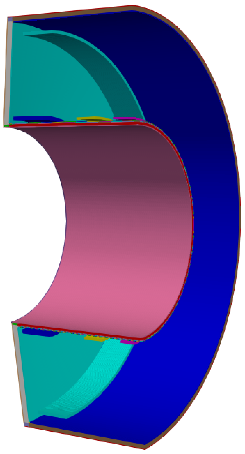
Based on the structure shown in Figure 2 and the symmetry simplifications illustrated in Figure 5, a quarter 3D model was established, as depicted in Figure 6. It displays the 3D simplified model adopted for simulation calculation. Considering the confidentiality of commercial product parameters, the model is established with scaled and reasonably simplified dimensions based on the real structure.Meanwhile, the dimensional parameters of the model in Figure 6 refer to those listed in

Table 1. Dimensions of the dry cool superconducting MRI system model.

Name	Size/mm
Radius of OVC inner bore	468
Thickness of OVC inner bore	12
Radius of OVC outer shell	960
Thickness of OVC outer shell	8
Thickness of OVC end	8
Z-direction length of OVC	1500
Radius of thermal shield inner bore	474
Thickness of thermal shield inner bore	8
Radius of thermal shield outer shell	930
Thickness of thermal shield outer shell	8
Thickness of thermal shield end	4
Z-direction length of GC	130
Z-direction length of thermal shield	1380
Radius of main GC	400
Radius of shield GC	410

.

Meanwhile, the code and program were developed based on the coupling formulas derived in Section 3, combined with finite element theory. Both strong coupling and weak coupling calculations of the electromagnetic–mechanical multi-physics field were performed on this model and program. In the weak coupling calculation process, fixed constraint boundary conditions were applied to all components; i.e., the displacement $\mathit{u}$ was always set to zero. This ensured that all metal components did not experience displacement under the Lorentz force, thereby preventing the generation of secondary eddy currents. Consequently, only primary eddy currents existed in the weak coupling process. A comparison between strong coupling and weak coupling is shown in Figure 7. It can be intuitively seen from Figure 7 the difference between strong coupling and weak coupling. Strong coupling considers the vibration caused by the Lorentz force, which further generates secondary eddy currents with kinetic energy involved. In contrast, weak coupling ignores this effect, vibrations are constrained by boundary conditions such that the kinetic energy is zero, and no secondary eddy currents exist accordingly.

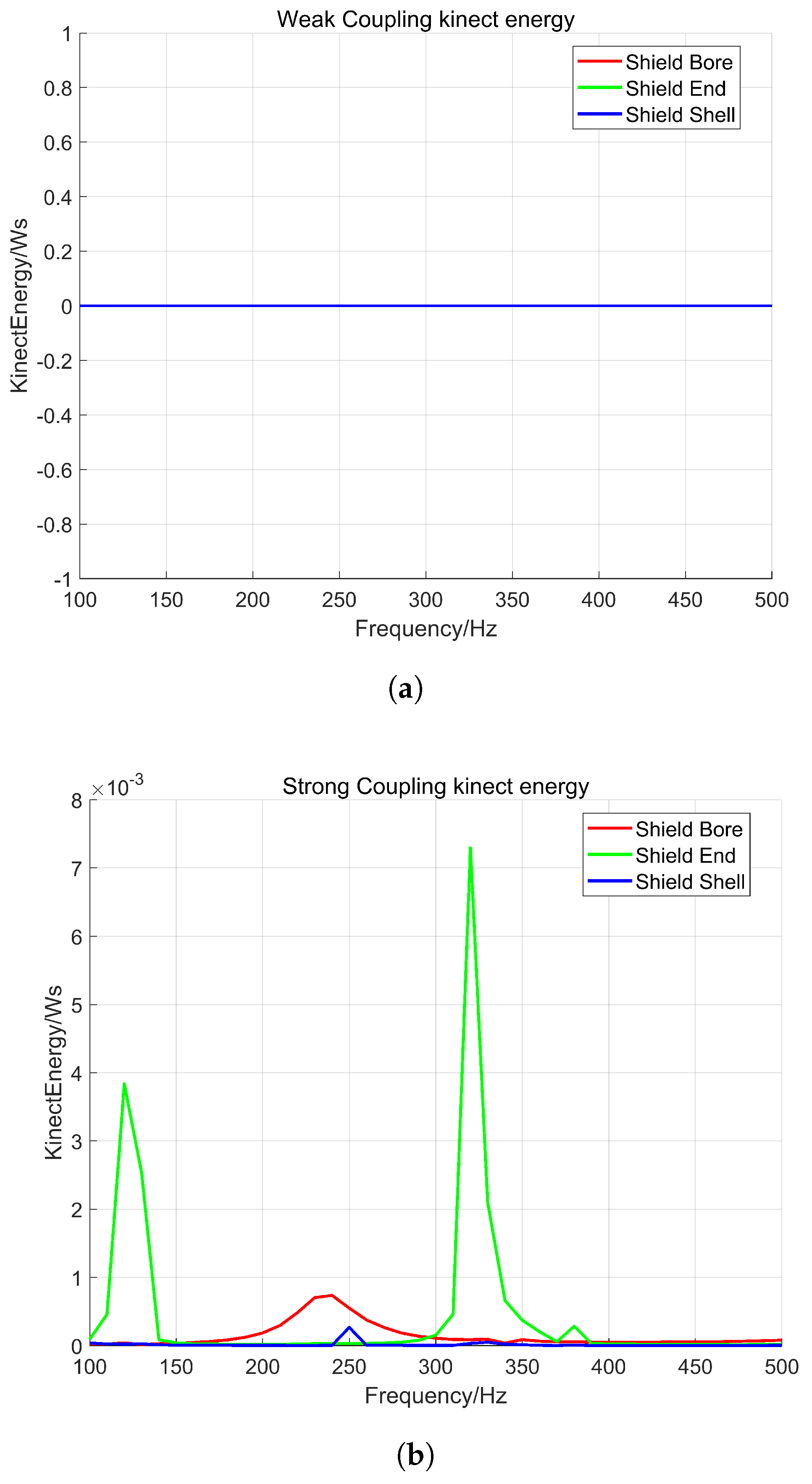
At this point, taking 100–500 Hz as an example, the kinetic energy on each component of the thermal shield under different coupling was observed. In Figure 8a, it can be seen that the kinetic energy is zero in all cases, indicating that the constraint on displacement $\mathit{u}$ in the weak coupling process has been successfully achieved. In the strong coupling calculation without the fixed constraint boundary conditions, the kinetic energy of each component is shown in Figure 8b. It can be observed that each component experienced displacement under the influence of Lorentz force.

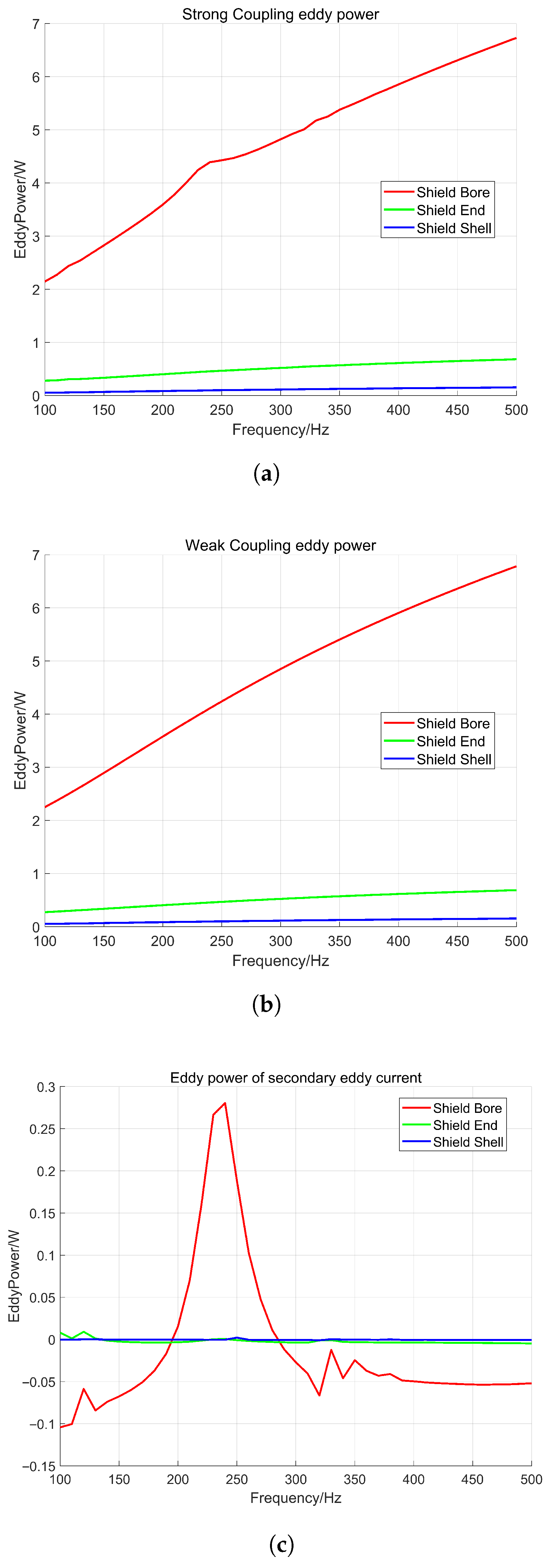
Then, the eddy current power of each component under strong and weak coupling conditions is obtained, as shown in Figure 9a,b.

Based on the comparison between strong and weak coupling shown in Figure 7, the difference between the two coupling conditions is attributed to the secondary eddy current. Therefore, the eddy power generated solely by the secondary eddy current is obtained by subtracting the calculation results of the two conditions, as presented in Figure 9c.

Based on the aforementioned calculation results, the generation and influence of the secondary eddy current are analyzed and discussed in the following section.

4.2. Analysis and Discussion

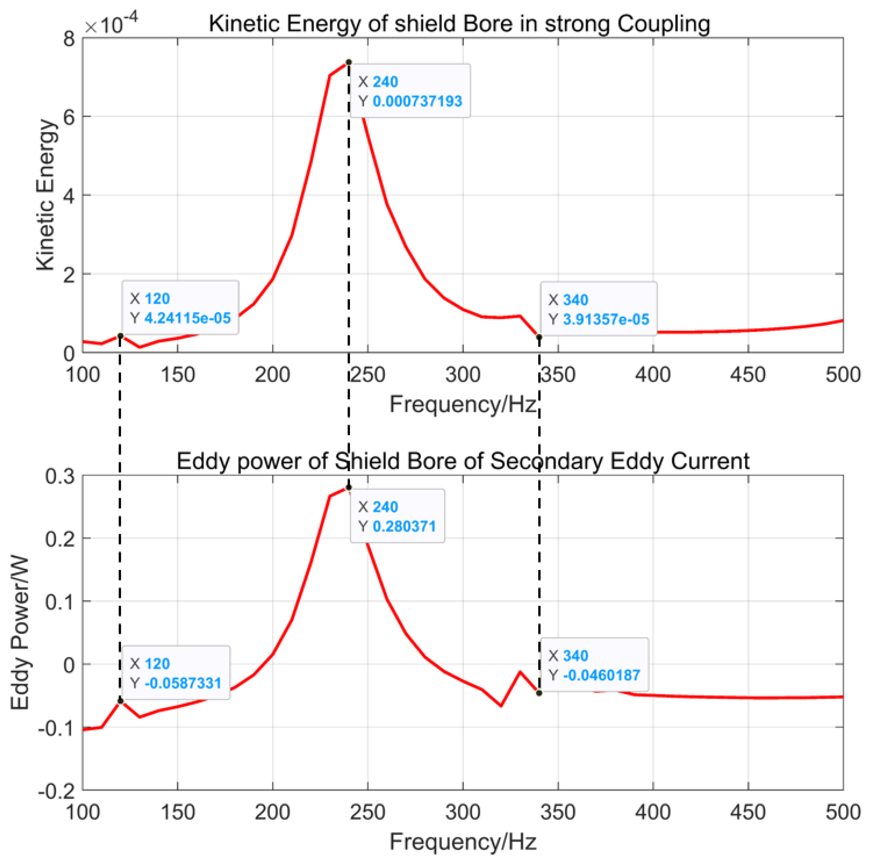
As illustrated in Figure 9c, the eddy power of the secondary eddy current on the shield bore is the most significant. Therefore, the shield bore is selected as the subject for in-depth analysis. A comparison between the kinetic energy of the shield bore in Figure 8b and its eddy power in Figure 9c is presented in Figure 10. The results show that the variation trends of the waveforms are completely consistent, with peaks appearing at the same frequency points (120 Hz, 240 Hz, and 340 Hz). This finding corroborates the preceding theoretical analysis, confirming that the secondary eddy current is primarily generated by the motion of components under the influence of the Lorentz force.

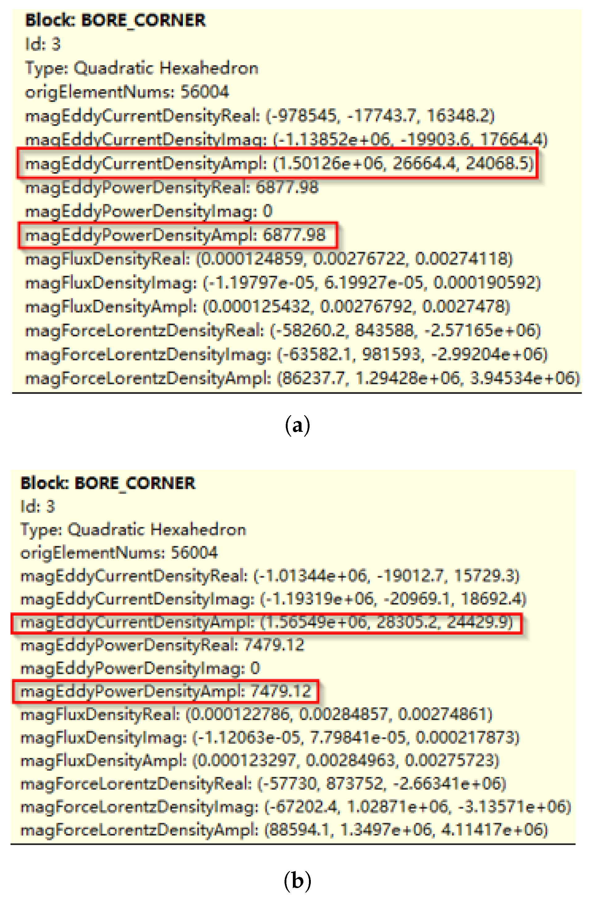
At this point, a specified element on the shield bore is selected for the numerical calculation of the eddy power of the secondary eddy current on that element. Taking 100 Hz as an example, the results extracted using mesh reading software are shown in Figure 11a,b. All data presented in the figures are in SI units.

The eddy power attributed to the secondary eddy current is obtained by directly subtracting the eddy power under weak coupling from that under strong coupling, yielding the following result:

$$\Delta P=P_{SC}-P_{WC}=-601.14\mathrm{W}/{\mathrm{m}}^3$$

(28)

However, if vector calculations are performed using the eddy current results presented in the figures, with the real and imaginary parts of the secondary eddy current calculated separately, the eddy power induced by the secondary eddy current is as follows:

$$J_{2nd}^{Re}=J_{SC}^{Re}-J_{WC}^{Re}$$

(29)

$$J_{2nd}^{Im}=J_{SC}^{Im}-J_{WC}^{Im}$$

(30)

$$\begin{array}{cc}\hfill P_{2nd}& =\frac{1}{2}·\frac{1}{\sigma }·{\left|J_{2nd}^{Ampl}\right|}^2\hfill \\ \hfill & =\frac{1}{2}·\frac{1}{\sigma }·\left({\left(J_{2nd}^{Re}\right)}^2+{\left(J_{2nd}^{Im}\right)}^2\right)\hfill \\ \hfill & =12.84\mathrm{W}/{\mathrm{m}}^3\hfill \end{array}$$

(31)

Based on the comparative analysis of the strong and weak coupling processes presented above, the vector superposition relationship of the eddy currents can be expressed as:

$$\begin{array}{cc}\hfill {\left|J_{SC}\right|}^2=& |J_{WC}+J_{2nd}{|}^2\hfill \\ \hfill & =|J_{WC}{|}^2+{\left|J_{2nd}\right|}^2+2\mathrm{Re}(J_{WC}·J_{2nd}^{*})\hfill \end{array}$$

(32)

Then, the eddy power induced by the secondary eddy current is calculated as:

$$\begin{array}{cc}\hfill \Delta P& =P_{\mathrm{SC}}-P_{\mathrm{WC}}=\frac{1}{2\sigma }\left(|J_{2nd}{|}^2+2\mathrm{Re}\left(J_{\mathrm{WC}}·J_{2nd}^{*}\right)\right)\hfill \\ \hfill & =P_{2nd}+\frac{1}{\sigma }\mathrm{Re}\left(J_{\mathrm{WC}}·J_{2nd}^{*}\right)\hfill \end{array}$$

(33)

where

$$\frac{1}{\sigma }\mathrm{Re}\left(J_{\mathrm{WC}}·J_{2nd}^{*}\right)=-613.8\mathrm{W}/{\mathrm{m}}^3$$

(34)

Under this condition,

$$\Delta P=12.84-613.8=-600.96\mathrm{W}/{\mathrm{m}}^3$$

(35)

It can be observed from Equations (28) and (35) that the eddy power induced by the secondary eddy current, calculated using the two methods, is in close agreement. Therefore, from the perspective of vector analysis, it can be concluded that the eddy power generated solely by the secondary eddy current is negligible, whereas the eddy power resulting from the coupling effect between the secondary and primary eddy currents is substantial and plays a dominant role.

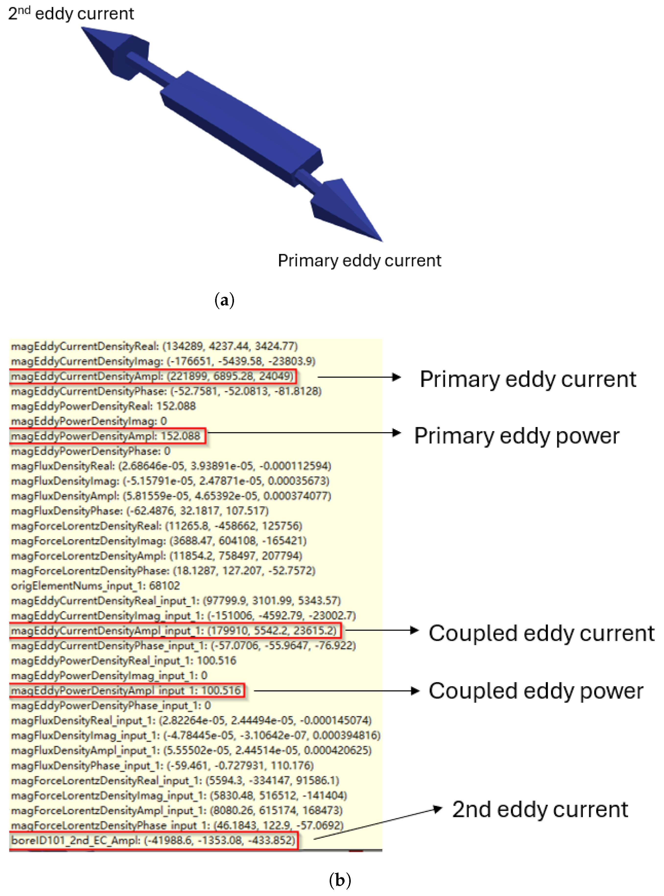
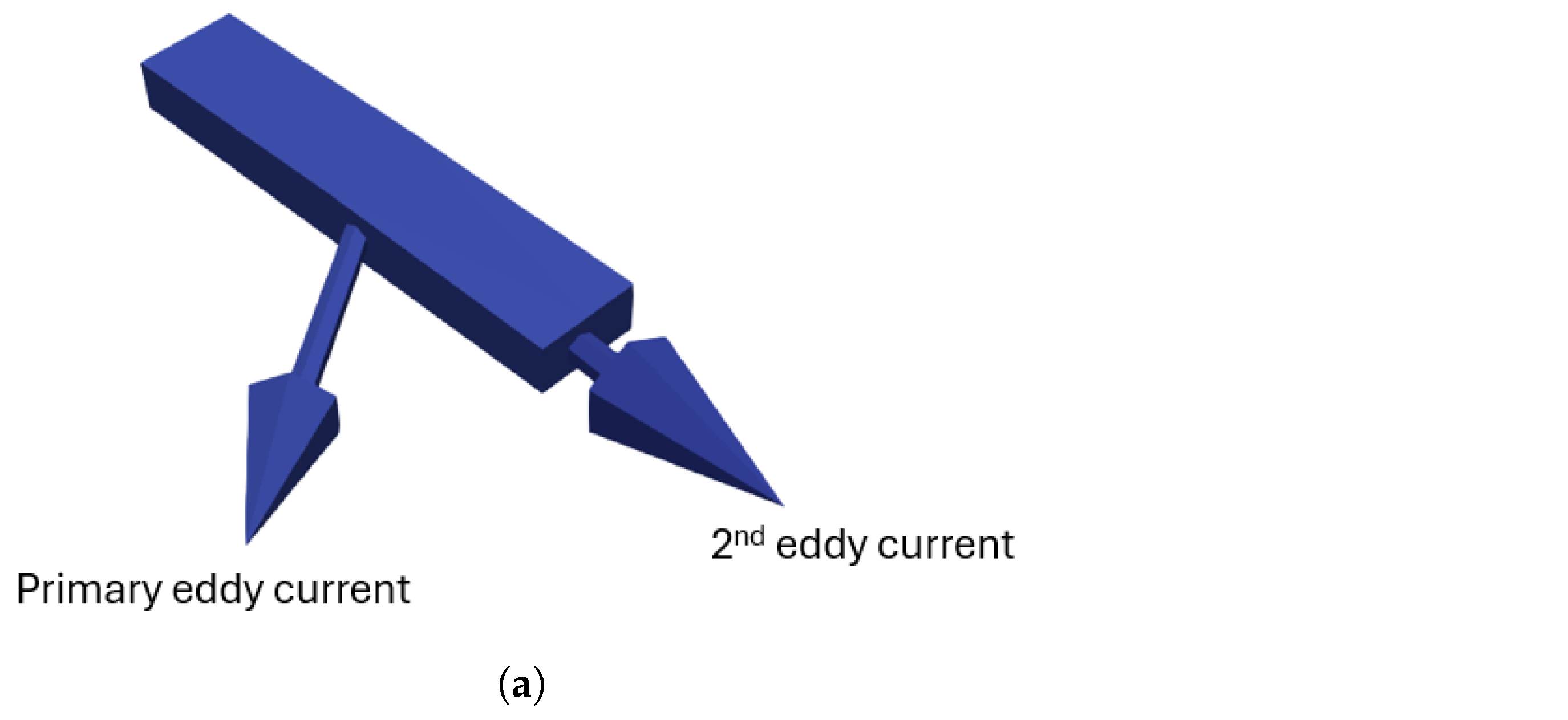
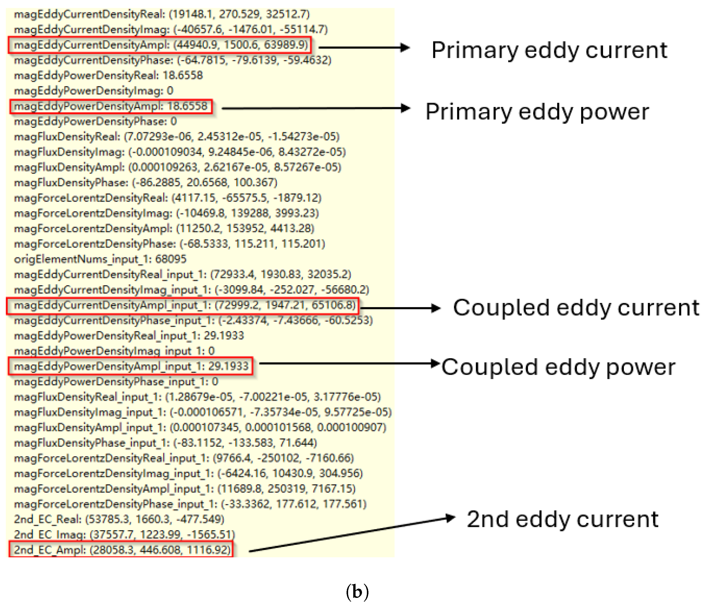
The directionality of the secondary eddy current at different frequencies is then discussed. Based on Figure 9c, two frequencies are selected: 190 Hz, where the eddy power of the secondary eddy current is negative, and 240 Hz, where it is positive. The results from the two coupling conditions are compiled together using mesh reading software, as presented in Figure 12a,b and Figure 13a,b.

Employing the calculation procedure from Equation (28) to Equation (35), the eddy power attributed to the secondary eddy current is calculated separately. It can be observed that for the selected element, the eddy power induced by the secondary eddy current is negative at 190 Hz. As shown in Figure 12a, the direction of the secondary eddy current is almost completely opposite to that of the primary eddy current at this frequency, exerting a suppressing effect and thus resulting in negative eddy power. Conversely, at 240 Hz, the eddy power induced by the secondary eddy current is positive. Figure 13a illustrates that the secondary eddy current has a component in the same direction as the primary eddy current, leading to a positive superposition effect and consequently generating positive eddy power. That is to say, at 190 Hz, the coupled eddy power (100.516) is lower than the uncoupled eddy power (152.068), because the direction of the secondary eddy current is opposite to that of the primary eddy current, resulting in a counteractive effect. At 240 Hz, the coupled eddy power (29.1933) is higher than the uncoupled eddy power (18.6558), since the secondary eddy current is in the same direction as the primary eddy current and produces a superimposed effect.

5. Conclusions

This study investigates eddy currents in a dry cool superconducting MRI system via strong and weak coupling analysis methods for electromagnetic and mechanical fields. First, the generation mechanism of secondary eddy currents is theoretically analyzed. Based on the force symmetry acting on the magnet, the 3D model is simplified, and the formulation for the strong coupling process is derived from both mechanical and electromagnetic perspectives, yielding a system of strong coupling matrix equations with higher-order terms and negligible quantities omitted or simplified. The simplified 3D model is then solved using these matrix equations.

In the simulation, weak coupling is achieved by constraining the displacement of each component, and the results are validated using kinetic energy. The frequency-dependent eddy power of secondary eddy currents is obtained by subtracting weak coupling results from strong coupling results; comparison with the kinetic energy spectrum confirms that secondary eddy currents are generated by the vibration of the shield bore.

Furthermore, a single element is selected for numerical calculation and verification of secondary eddy current power. Vector analysis shows that the eddy power generated solely by secondary eddy currents is minimal, with the dominant contribution coming from the coupling between primary and secondary eddy currents. Additionally, the direction of eddy current vectors on the element explains the sign variation (positive or negative) of the eddy power induced by secondary eddy currents at different frequencies.

Overall, in the dry cool superconducting MRI system, the magnetic field on the superconducting coil originates from eddy current emissions. Primary eddy currents arise from the stray field of the gradient coil (GC), while secondary eddy currents are generated by the motion-induced electromotive force resulting from the vibration of the thermal shield bore under the Lorentz force.

Future research can apply these findings to the optimal design of such magnets. It is recommended to design relevant experiments for further validation and to consider additional metallic structures within the magnet.

References

1. Niu, C.Q. Research on Optimization Methods for Magnetic Resonance Imaging Gradient Systems. Ph.D. Thesis, University of Chinese Academy of Sciences, Beijing, China, 2020. [Google Scholar]
2. Plonsey, R.; Collin, R.E. Principles and Applications of Electromagnetic Fields; McGraw-Hill Book Company, Inc.: New York, NY, USA, 1961. [Google Scholar]
3. Badea, E.A.; Craiu, O. Eddy current effects in MRI superconducting magnets. IEEE Trans. Magn. 1997, 33, 1330–1333. [Google Scholar] [CrossRef]
4. Iwasa, Y.; Bascunan, J.; Hahn, S. High-temperature superconducting magnets for NMR and MRI: R&D activities at the MIT francis bitter magnet laboratory. IEEE Trans. Appl. Supercond. 2010, 20, 718–721. [Google Scholar]
5. Edelstein, W.A.; Hedeen, R.A.; Mallozzi, R.P. Making MRI quieter. Magn. Reson. Imaging 2002, 20, 155–163. [Google Scholar] [CrossRef] [PubMed]
6. Edelstein, W.A.; Kidane, T.K.; Taracila, V. Active-passive gradient shielding for MRI acoustic noise reduction. Magn. Reson. Med. 2005, 53, 1013–1017. [Google Scholar] [CrossRef]
7. Wang, Y.; Liu, F.; Zhou, X. A numerical study of the acoustic radiation due to eddy current cryostat interactions. Med. Phys. 2017, 44, 2196–2206. [Google Scholar] [CrossRef]
8. Bernstein, M.A.; King, K.F.; Zhou, X.J. Handbook of MRI Pulse Sequences; Elsevier Academic Press: Burlington, MA, USA; San Diego, CA, USA; London, UK, 2004. [Google Scholar]
9. Liu, Q.; Hughes, D.G.; Allen, P.S. Quantitative characterization of the eddy current fields in a 40 cm bore superconducting magnet. Magn. Reson. Med. 1994, 31, 73–76. [Google Scholar] [CrossRef]
10. You, X.F. Research on Optimal Design of Gradient and Shim Coils for Magnetic Resonance Imaging System. Ph.D. Thesis, University of Chinese Academy of Sciences, Beijing, China, 2013. [Google Scholar]
11. Henkelman, R.M.; Bronskill, M.J. Artifacts in magnetic resonance imaging. Magn. Reson. Med. 1987, 2, 126–256. [Google Scholar]
12. Spees, W.M.; Buhl, N.; Sun, P. Quantification and compensation of eddy-current-induced magnetic-field gradients. J. Magn. Reson. 2011, 212, 116–123. [Google Scholar] [CrossRef]
13. Jezzard, P.; Barnett, A.S.; Pierpaoli, C. Characterization of and correction for eddy current artifacts for echo planar diffusion imaging. Magn. Reson. Med. 1998, 39, 801–812. [Google Scholar] [CrossRef] [PubMed]
14. Trakic, A.; Liu, F.; Lopez, H.S. Longitudinal gradient coil optimization in the present of transient eddy currents. Magn. Reson. Med. 2007, 57, 1119–1130. [Google Scholar] [CrossRef] [PubMed]
15. Chung, Y.; Galayda, J. Effect of Eddy Current in the Laminations on the Magnetic Field; Argonne National Laboratory: Lemont, IL, USA, 1992.
16. Agarwal, P.D. Eddy-current losses in solid and laminated iron. IEEE Trans. Commun. Electron. 1959, 78, 169–181. [Google Scholar] [CrossRef]
17. Kinanen, I.V. Arrangement to Minimize Eddy Currents in MR Imagers. U.S. Patent 5555251A, 10 September 1996. [Google Scholar]
18. Wickliffe, G.D.; Morich, M.A.; Patrick, J.L. Filamentary Cold Shield for Superconducting Magnets. U.S. Patent 5280247A, 18 January 1994. [Google Scholar]
19. Dong, H. Simulation and Measurements of Transient Fields from Conductive Plates of Shielded Room for SQUID-Based Ultralow Field Magnetic Resonance Imaging. IEEE Trans. Appl. Supercond. 2019, 29, 1601605. [Google Scholar] [CrossRef]
20. Valsamis, J.J.; Dubovan, P.I.; Baron, C.A. Characterization and Correction of Time-Varying Eddy Currents for Diffusion MRI. Magn. Reson. Med. 2021, 87, 2209–2223. [Google Scholar] [CrossRef]
21. Kar, S. Quench Induced Eddy Current and Mechanical Stresses in the Bobbin and Thermal Shield of the 1.5 T MRI Magnet System. IEEE Trans. Appl. Supercond. 2021, 31, 4400907. [Google Scholar] [CrossRef]
22. Alsharafi, S.S.; Badawi, A.; El-Sharkawy, A. Eddy currents analysis methods for an MRI longitudinal gradient coil. Magn. Reson. Med. 2023, 90, 2158–2174. [Google Scholar] [CrossRef] [PubMed]
23. Takrimi, M.; Atalar, E. Minimization of eddy power loss in the cryostat for a z-gradient array coil driven by an arbitrary pulse sequence: An electromagnetic approach. Magn. Reson. Med. 2024, 91, 1225–1238. [Google Scholar] [CrossRef] [PubMed]
24. Lee, S.K.; Tarasek, M.; Spence, L.D.K. Eddy Current Heating of Metallic Shells and Plates: Application to Gradient-Induced Conductor Heating in MRI. IEEE Trans. Magn. 2024, 60, 5100310. [Google Scholar] [CrossRef]
25. Lee, S.K.; Hua, Y. Theory and mitigation of motional eddy current in high-field eddy current shielding. J. Appl. Phys. 2024, 136, 024504. [Google Scholar] [CrossRef]
26. Zhang, Y.; Kong, X.; He, W.; Xu, Z. Eddy Current Characterization Using Efficient Finite Element Analysis for Z-Gradient Coils in a Low-Field MRI Scanner. IEEE Trans. Instrum. Meas. 2025, 74, 4003909. [Google Scholar] [CrossRef]
27. Zhao, Z. Study and Applications on Transient Field of Heterogeneous Simulation System for Electromagnetic-Mechanical Coupling. Ph.D. Thesis, Zhejiang University, Hangzhou, China, 2011. [Google Scholar]
28. Wang, A.L.; Zhong, Z. Global coupling modeling method and simulation research of complex electromechanical systems. J. Mech. Eng. 2003, 39, 1–5. [Google Scholar] [CrossRef]
29. Kolluri, D.K.; Boidin, X.; Desplanques. Effect of natural graphite particle size in friction materials on thermal localization phenomenon during stop-braking. Wear 2010, 268, 1472–1482. [Google Scholar] [CrossRef]
30. Li, H.F.; Zhou, L.; Zhou, D. Study on wind pressure distribution and wind-induced response of saddle-shaped cable-membrane structures considering fluid-structure interaction effects. J. Shanghai Jiaotong Univ. 2009, 43, 967–971. [Google Scholar]
31. Su, B.; Qian, R.J.; Yuan, X.F.; Yu, M. Fluid-structure coupling interface data transfer method using energy conservation and radial basis function interpolation. J. Xi’an Jiaotong Univ. 2009, 43, 114–119. [Google Scholar]
32. Liu, X.; Chen, X.Y. Electromechanical coupling simulation analysis of RF MEMS switches. J. Qingdao Univ. (Eng. Technol. Ed.) 2007, 22, 60–65. [Google Scholar]
33. Li, Y.; Yu, X.L.; Li, T. Finite element simulation of piston-cylinder transient coupling heat transfer. J. Zhejiang Univ. (Eng. Sci.) 2007, 41, 347–355. [Google Scholar]
Figure 1. Formation process of primary and secondary eddy currents.
Symmetry 18 00913 g001
Figure 2. Schematic cross-sectional diagram of the dry cool superconducting magnet structure.
Symmetry 18 00913 g002
Figure 3. Schematic diagram of the research process.
Symmetry 18 00913 g003
Figure 4. Schematic diagram of the Y-direction gradient coil (Y-GC) structure.
Symmetry 18 00913 g004
Figure 5. Schematic diagram of Lorentz force components in all directions of the thermal shield from different perspectives: (a) The X-direction component from the +Z perspective and three-dimensional perspective. (b) The Y-direction component from the +Z perspective and three-dimensional perspective. (c) The Z-direction component from the +X perspective and +Y perspective.
Symmetry 18 00913 g005
Figure 6. The quarter 3D model used in the simulation.
Symmetry 18 00913 g006
Figure 7. Comparison between strong coupling and weak coupling.
Symmetry 18 00913 g007
Figure 8. Kinetic energy of each shield component under different coupling: (a) The kinetic energy calculation results under weak coupling. (b) The kinetic energy calculation results under strong coupling.
Symmetry 18 00913 g008
Figure 9. Eddy power of each shield component under different coupling: (a) Eddy power of each shield component in the strong coupling. (b) Eddy power of each shield component in the weak coupling. (c) Eddy power of secondary eddy current.
Symmetry 18 00913 g009
Figure 10. The comparison between the kinetic energy of the shield bore and the eddy power of the secondary eddy current.
Symmetry 18 00913 g010
Figure 11. A specified element is selected to perform numerical calculation of the eddy power of the secondary eddy current by reading its physical quantities: (a) The calculation results of various physical quantities for this element under strong coupling. (b) The calculation results of various physical quantities for this element under weak coupling.
Symmetry 18 00913 g011
Figure 12. The eddy current direction of a specific element at 190 Hz and the corresponding coupling calculation results: (a) The directions of the primary eddy current and the secondary eddy current. (b) The coupling calculation results.
Symmetry 18 00913 g012
Figure 13. The eddy current direction of a specific element at 240 Hz and the corresponding coupling calculation results: (a) The directions of the primary eddy current and the secondary eddy current. (b) The coupling calculation results.
Symmetry 18 00913 g013aSymmetry 18 00913 g013b