A Hankel Determinant—Driven Framework for Medical Image Enhancement Using Bi-Univalent Functions

Abstract

This study introduces a new approach to image enhancement by integrating ideas from geometric function theory with modern computer vision techniques. A specific subclass $\mathcal{B}(\hslash )$ of bi-univalent functions is constructed, and its associated Hankel determinants are employed to design convolution-based enhancement filters. These determinants are incorporated as adaptive weights within the filtering process to improve image quality. The effectiveness of the proposed framework is assessed using widely accepted performance measures, including PSNR, SSIM, MSE, standard deviation, and Pearson correlation coefficient. Experimental results on various medical imaging datasets demonstrate clear improvements compared to existing methods. The proposed method is evaluated on different medical images obtained from publicly available Kaggle and Radiopaedia datasets. Quantitative comparison of the proposed method against two histogram-based enhancement methods, QDHE and CLAHE, demonstrates substantial improvements across all quality metrics, achieving superior image enhancement with better preservation of fine structural details. An ablation study confirms that Hankel weights contribute approximately 4.5 dB and directional fusion contributes 2.8 dB to the average PSNR. The findings demonstrate a quantifiable connection between the theory of Hankel determinants and practical image processing applications.

1. Introduction

Let $\mathtt{Q}$ be the collection of analytic functions ($\mathtt{Afs}$) within the open unit disk $\mathtt{U}=\{\mathtt{z}:|\mathtt{z}|<1\}$, which can be written as:

$$\mathtt{D}\left(\mathtt{z}\right)=\mathtt{z}+{\displaystyle \sum _{n\geqq 2}}{g}_n{\mathtt{z}}^n,\mathtt{z}\in \mathtt{U}$$

(1)

and which have the properties $\mathtt{D}\left(0\right)=0$, $\mathtt{D}\left(0\right)=1$. In this set $\mathtt{Q}$ we can consider a subset S consisting of univalent functions ($\mathtt{Ufs}$) in $\mathtt{U}$. 

There are multiple subfamilies of S, including bounded turning function ($\mathtt{BTfs}$), convex function ($\mathtt{Cfs}$), starlike functions ($\mathtt{Sfs}$) defined by specific geometric features

$$\Re \left[{\mathtt{D}}^{\prime }\left(\mathtt{z}\right)\right]>0;\Re \left[{\displaystyle \frac{{\left(\mathtt{z}{\mathtt{D}}^{\prime }\left(\mathtt{z}\right)\right)}^{\prime }}{{\mathtt{D}}^{\prime }\left(\mathtt{z}\right)}}\right]>0;\Re \left[{\displaystyle \frac{\mathtt{z}{\mathtt{D}}^{\prime }\left(\mathtt{z}\right)}{\mathtt{D}\left(\mathtt{z}\right)}}\right]>0.$$

There are also numerous other variations that have been investigated for their geometric properties as documented in the extant literature.

The symbol $\mathcal{CV}\left(\tau \right)$ represents the $\mathtt{Cfs}$ of order $\tau$$(0\le \tau <1)$, and $\mathcal{ST}\left(\tau \right)$ represents the $\mathtt{Sfs}$ of order $\tau$. These are two important examples of S subclasses that have received a great deal of attention. The details can be found in [1]. The more recent work in the $\mathtt{GFT}$ has been done by considering functions whose values are determined by joining the first coefficients of functions in the class $\mathtt{Q}$. It is proven that if $\mathtt{D}\in S$ then $|g_n|$ is bounded by n. These bounds on the coefficients reveal information about the geometric properties of the functions

Now, if ${\mathtt{D}}_1,{\mathtt{D}}_2\in \mathtt{Q}$, we write ${\mathtt{D}}_1\left(\mathtt{z}\right)\prec {\mathtt{D}}_2\left(\mathtt{z}\right)$ and the following conditions being satisfied: $\omega \in \mathtt{Q}$, $\omega \left(0\right)=0$, $\left|\omega \right(\mathtt{z}\left)\right|<1$, and ${\mathtt{D}}_1\left(\mathtt{z}\right)={\mathtt{D}}_2\left(\omega \left(\mathtt{z}\right)\right)$, the function ${\mathtt{D}}_1$ is subordinate to ${\mathtt{D}}_2$.

We know from the popular Theorem (one-quarter Theorem) introduced by Koebe which proves that the image of $\mathtt{U}$ under every $\mathtt{Ufs}$ contains a disk of radius ${\displaystyle \frac{1}{4}}$. Furthermore, we can say that for every $\mathtt{D}\in S$, there exists an inverse ${\mathtt{D}}^{-1}$ which is shown below:

$${\mathtt{D}}^{-1}\left(\mathtt{D}\left(\mathtt{z}\right)\right)=\mathtt{z}$$

$$\mathrm{and}\mathtt{D}\left({\mathtt{D}}^{-1}\left(\mathtt{l}\right)\right)=\mathtt{l}\left(\right|\mathtt{l}|<s_0\left(\mathtt{D}\right);s_0\left(\mathtt{D}\right)\ge 4^{-1})$$

with

$${\mathtt{D}}^{-1}\left(\mathtt{l}\right)=\mathtt{l})=\mathtt{l}-g_2{\mathtt{l}}^2+(-g_3+2g_2^2){\mathtt{l}}^3-(g_4-5g_2{g}_3+5g_2^3){\mathtt{l}}^4+\cdots .$$

(2)

We can now indicate by E the set of every bi-univalent functions ($\mathtt{Bfs}$) in $\mathtt{U}$, which we have below:

$$E=\{\mathtt{D}\in \mathtt{Q}:{\mathtt{D}}^{-1},\mathtt{D}\in S\}.$$

Brannan and Taha [2] presented bi-$\mathtt{Sfs}$ of order $\tau$ ($0<\tau \le 1$), indicated by ${\mathcal{ST}}_{\Theta }\left(\tau \right)$, and bi-$\mathtt{Cfs}$ of order $\tau$, indicated by ${\mathcal{CV}}_{\Theta }\left(\tau \right)$. They provided initial, though not precise, estimates for the absolute values of the first two Taylor-Maclaurin coefficients, $|g_2|$ and $|g_3|$, for both ${\mathcal{ST}}_{\Theta }\left(\tau \right)$ and ${\mathcal{CV}}_{\Theta }\left(\tau \right)$ [2,3,4].

However, determining exact estimates for subsequent Taylor-Maclaurin coefficients, $|g_n|$ (for $n\in \mathbb{N}\setminus \{1,2\}$), remains an unresolved problem. Following extensive research into various interesting subclasses of $\Theta$, many authors (see [5,6,7,8,9,10] and references cited therein) have concluded that the initial estimations for $|g_2|$ and $|g_3|$ are not sharp. 

Using the function $\mathtt{D}\left(\mathtt{z}\right)$ from Equation (1), we can define the $n^{th}$ Hankel determinant introduced in 1973 by Noonan and Thomas [11] when $n\ge 1$, $\mathtt{q}\ge 1$, and $g_1=1$.

$${\mathcal{H}}_n\left(\mathtt{q}\right)=\left|\begin{array}{ccccc}{g}_{\mathtt{q}}& g_{\mathtt{q}+1}& g_{\mathtt{q}+2}& \dots & g_{\mathtt{q}+n-1}\\ g_{\mathtt{q}+1}& g_{\mathtt{q}+2}& g_{\mathtt{q}+3}& \dots & g_{\mathtt{q}+n}\\ g_{\mathtt{q}+2}& g_{\mathtt{q}+3}& g_{\mathtt{q}+4}& \dots & g_{\mathtt{q}+n+1}\\ ⋮& ⋮& ⋮& \dots & ⋮\\ g_{\mathtt{q}+n-1}& g_{\mathtt{q}+n}& g_{\mathtt{q}+n+1}& \dots & g_{\mathtt{q}+2(n-1)}\end{array}\right|.$$

(3)

Setting $n=2$ and $\mathtt{q}=1$ in Equation (3), we derive the following expression:

$${\mathcal{H}}_2\left(1\right)=\left|\begin{array}{cc}1& g_2\\ g_2& g_3\end{array}\right|=|g_3-g_2^2|.$$

(4)

Furthermore, the Hankel determinant of order two for bi-$\mathtt{Sfs}$ and bi-$\mathtt{Cfs}$ is given by [12,13]:

$$|{\mathcal{H}}_2\left(2\right)|=|g_2{g}_4-g_3^2|.$$

(5)

This expression can be generalized as,

$$|g_3-\rho g_2^2|$$

(6)

where $\rho$ represents a number that can be either real or complex. For more instances on $|g_3-\rho g_2^2|$ see [14].

Also, we have the third Hankel determinant, which has been studied by [15] can be written as follows:

$${\mathcal{H}}_3\left(1\right)=\left|\begin{array}{ccc}{g}_1& g_2& g_3\\ g_2& g_3& g_4\\ g_3& g_4& g_5\end{array}\right|$$

(7)

From (7), applying the triangle inequality, we obtain the following expression:

$$|{\mathcal{H}}_3\left(1\right)|\le |g_3-g_2^2\left|\right|g_5|+|g_4-g_2{g}_3\left|\right|g_4|+|g_2{g}_4-g_3^2\left|\right|g_3|.$$

(8)

The Hankel determinant is crucial in singularity theory [16] and is useful for examining power series with integer coefficients (see [17]). Many researchers have determined maximum limits for ${\mathcal{H}}_n\left(\mathtt{q}\right)$ with varying values of k and c in different categories of $\mathtt{Afs}$ (refer to [18,19,20,21,22,23,24,25], for more information).

Image enhancement plays a central role in medical image analysis, where the accurate interpretation of structural details is essential for reliable diagnosis [26,27]. However, medical images such as ultrasound, MRI, and CT scans are often affected by low contrast, speckle noise, and non-uniform illumination, which obscure fine anatomical features [26]. Conventional enhancement techniques, including histogram equalization and Retinex-based methods [28,29] offer partial improvements but often suffer from noise amplification and loss of structural fidelity. More recent deep learning approaches achieve superior performance but require large annotated datasets and significant computational resources, limiting their practical deployment in resource-constrained environments.

In parallel, geometric function theory (GFT) has emerged as a powerful mathematical framework for analyzing analytic and univalent functions through their coefficient structures [30,31]. In particular, Hankel determinants capture higher-order interactions among coefficients and have been extensively studied in connection with growth, distortion, and stability properties of analytic functions [11,15,18]. Despite their rich theoretical significance, the potential of these structures in practical image processing applications remains largely unexplored.

Motivated by this gap, the present work establishes a novel connection between the theory of bi-univalent functions and digital image enhancement. This study introduces a novel subclass of functions, denoted as $\mathtt{Bfs}$, extending prior research that explored various subclasses of $\mathtt{Afs}$ and $\mathtt{Bfs}$ within the domain $\mathtt{U}$. Previous investigations often focused on the second Hankel determinant for functions in $\mathtt{Bfs}$, as exemplified by the work in [32,33]. The primary goal of this research is to define a distinct subclass of $\mathtt{Bfs}$ and, crucially, to determine bounds for its third Hankel determinant. Consequently, this work establishes fresh limitations for the estimated values of the third Hankel determinant specific to the class $\mathcal{B}(\hslash )$. These determinants are then systematically embedded into directional convolution kernels, enabling the extraction and enhancement of structural features in images. Similar ideas of utilizing analytic function coefficients in image processing have recently been explored in [34,35,36,37,38], which further motivates the present framework.

Recent advances in medical image enhancement have increasingly relied on Retinex-based frameworks, variational denoising models, transformer-based architectures, and lightweight convolutional neural networks for improving contrast and suppressing noise in low-quality medical scans. Retinex-inspired methods provide illumination correction and local contrast adaptation, whereas deep learning approaches achieve impressive enhancement performance through data-driven feature extraction. However, many of these approaches require extensive training datasets, parameter optimization, and high computational resources, which may limit their applicability in real-time or resource-constrained medical environments. Moreover, low-light image enhancement approaches have increasingly focused on feature fusion and attention-guided architectures. The virtual exposure-based enhancement method proposed in 2023 utilizes exposure reconstruction and multi-scale fusion to improve illumination consistency and detail preservation. Similarly, the Convolutional Dense Attention-Guided Network (CDAN) employs dense feature propagation, attention modules, and skip connections to enhance structural information and perceptual quality in low-light images. These approaches demonstrate the effectiveness of information transfer and attention mechanisms in preserving image details under challenging illumination conditions [39].

Unlike these deep learning-based approaches, the proposed framework achieves enhancement through analytically derived Hankel determinant structures and coefficient bounds, providing a mathematically interpretable and lightweight alternative for structural enhancement.

2. A Set of Lemmas

The following lemmas are used to derive the main results.

Lemma 1 

([30]). Suppose that $\mathtt{u}\in \mathcal{P}$ is of series form

$$\mathtt{u}\left(\mathtt{z}\right)=1+{\displaystyle \sum _{n=1}^{\infty }}{\mathtt{u}}_n{\mathtt{z}}^n$$

(9)

where $\Re \left(\mathtt{u}\right(\mathtt{z}\left)\right)>0$ and $\mathtt{z}\in \mathtt{U}$, so

$$|{\mathtt{u}}_n|\le 2,n\in \mathbb{N}.$$

Lemma 2 

([40]). Assume that $\mathtt{u}\in \mathcal{P}$ has the form of a series given in (9), and $\Re \left(\mathtt{u}\right(\mathtt{z}\left)\right)>0$ where $\mathtt{z}$ in $\mathtt{U}$, so

$${\mathtt{u}}_2={\displaystyle \frac{{\mathtt{u}}_1^2+(4-{\mathtt{u}}_1^2)e_1}{2}},$$

$${\mathtt{u}}_3={\displaystyle \frac{{\mathtt{u}}_1^3+2(4-{\mathtt{u}}_1^2){\mathtt{u}}_1{e}_1-(4-{\mathtt{u}}_1^2){\mathtt{u}}_1{e}_1^2+2(4-{\mathtt{u}}_1^2)(1-|e_1{|}^2)\mathtt{z}}{4}}.$$

3. Main Results

In this section, we introduce a subclass of bi-univalent functions as follows:

Definition 1.

Let $\mathtt{D}\left(\mathtt{z}\right)$ be a function in the class E. We say that $\mathtt{D}$ belongs to the subclass $\mathcal{B}(\hslash )$ if the following conditions are satisfied:

$$\Re \left({\displaystyle \frac{2\mathtt{z}{\mathtt{D}}^{\prime }\left(\mathtt{z}\right)}{\mathtt{D}\left(\mathtt{z}\right)-\mathtt{D}(-\mathtt{z})}}\right)>⋋,\mathit{for}\mathit{all}\mathtt{z}\in \mathbb{U},$$

(10)

and

$$\Re \left({\displaystyle \frac{2\mathtt{l}{\mathtt{G}}^{\prime }\left(\mathtt{l}\right)}{\mathtt{l})-\mathtt{G}(-\mathtt{l})}}\right)>⋋,\mathit{for}\mathit{all}\mathtt{l}\in \mathbb{U},$$

(11)

where $\mathtt{G}$ denotes the inverse of $\mathtt{D}$, $\mathbb{U}$ is the open unit disk, and $0\le ⋋<1$.

Theorem 1.

Let $\mathtt{D}\in \mathcal{B}(\hslash )$, where $0\le ⋋<1$. Then

$$|g_2{g}_4-g_3^2{|\le (1-⋋)}^2\left[{\displaystyle \frac{1}{4}}{(1-⋋)}^2+{\displaystyle \frac{1}{2}}\right].$$

(12)

Proof. 

Firstly, taking it from Equations (10) and (11), we yield:

$${\displaystyle \frac{2\mathtt{z}{\mathtt{D}}^{\prime }\left(\mathtt{z}\right)}{\mathtt{D}\left(\mathtt{z}\right)-\mathtt{D}(-\mathtt{z})}}=⋋+(1-⋋)\mathtt{u}\left(\mathtt{z}\right)$$

(13)

and

$${\displaystyle \frac{2\mathtt{l}\left(\mathtt{l}\right)}{\mathtt{G}\left(\mathtt{l}\right)-\mathtt{G}(-\mathtt{l})}}=⋋+(1-⋋)\mathtt{b}\left(\mathtt{l}\right)$$

(14)

where $\mathtt{u},\mathtt{b}\in \mathcal{P}$ and $\mathtt{z},\mathtt{l}\in \mathtt{U}$.

By assumption, we say that $\varrho :\mathtt{U}⟶\mathtt{U}$ and $\varsigma :\mathtt{U}⟶\mathtt{U}$, which are analytic functions alongside $\varrho \left(0\right)=0=\varsigma \left(0\right)$, $\left|\varrho \right(z\left)\right|<1$, $\left|\varsigma \right(\varpi \left)\right|<1$ satisfying the stipulated criteria:

$$\mathtt{u}\left(\mathtt{z}\right)={\displaystyle \frac{1+\varrho \left(\mathtt{z}\right)}{1-\varrho \left(\mathtt{z}\right)}}=1+\sum _{n\geqq 1}{\mathtt{u}}_n{\mathtt{z}}^n$$

and

$$\mathtt{b}\left(\mathtt{l}\right)={\displaystyle \frac{1+\varsigma \left(\mathtt{l}\right)}{1-\varsigma \left(\mathtt{l}\right)}}=1+\sum _{n\geqq 1}{\mathtt{b}}_n{\mathtt{l}}^n.$$

It follows that

$$⋋+(1-⋋)\mathtt{u}\left(\mathtt{z}\right)=1+\sum _{n\geqq 1}(1-⋋){\mathtt{u}}_n{\mathtt{z}}^n$$

(15)

and

$$⋋+(1-⋋)\mathtt{b}\left(\mathtt{l}\right)=1+\sum _{n\geqq 1}(1-⋋){\mathtt{b}}_n{\mathtt{l}}^n.$$

(16)

By expanding the LHS of Equation (13), we have:

$$\begin{array}{c}\hfill {\displaystyle \frac{2\mathtt{z}{\mathtt{D}}^{\prime }\left(\mathtt{z}\right)}{\mathtt{D}\left(\mathtt{z}\right)-\mathtt{D}(-\mathtt{z})}}=1+2g_2\mathtt{z}+2g_3{\mathtt{z}}^2+\left[4g_4-2g_2{g}_3\right]{\mathtt{z}}^3+\left[4g_5-2g_3^2\right]{\mathtt{z}}^4+\cdots \end{array}$$

(17)

and

$$\begin{array}{cc}\hfill {\displaystyle \frac{2\mathtt{l}\left(\mathtt{l}\right)}{\mathtt{l})--\mathtt{l})}}=& 1+(-2g_2)\mathtt{l}+\left[-2g_3+4g_2^2\right]{\mathtt{l}}^2+\left[16g_2{g}_3-4g_4-16g_2^3\right]{\mathtt{l}}^3\hfill \\ \hfill & +\left[-4g_5+10g_3^2+24g_2{g}_4-76g_2^2{g}_3+48g_2^4\right]{\mathtt{l}}^4+\cdots .\hfill \end{array}$$

(18)

Now, making use of (15) and (17) and taking note of the coefficients will yield:

$$\begin{array}{cc}\hfill 2g_2& =(1-⋋){\mathtt{u}}_1\hfill \end{array}$$

(19)

$$\begin{array}{cc}\hfill 2g_3& =(1-⋋){\mathtt{u}}_2\hfill \end{array}$$

(20)

$$\begin{array}{cc}\hfill 4g_4-2g_2{g}_3& =(1-⋋){\mathtt{u}}_3\hfill \end{array}$$

(21)

$$\begin{array}{cc}\hfill 4g_5-2g_3^2& =(1-⋋){\mathtt{u}}_4.\hfill \end{array}$$

(22)

Also, making use of (15) and (17) and taking note of the coefficients yields:

$$\begin{array}{cc}\hfill -2g_2& =(1-⋋){\mathtt{b}}_1\hfill \end{array}$$

(23)

$$\begin{array}{cc}\hfill -2g_3+4g_2^2& =(1-⋋){\mathtt{b}}_2\hfill \end{array}$$

(24)

$$\begin{array}{cc}\hfill 16g_2{g}_3-4g_4-16g_2^3& =(1-⋋){\mathtt{b}}_3\hfill \end{array}$$

(25)

$$\begin{array}{cc}\hfill -4g_5+10g_3^2+24g_2{g}_4-76g_2^2{g}_3+48g_2^4& =(1-⋋){\mathtt{b}}_4.\hfill \end{array}$$

(26)

From (19) and (23), we have

$${\displaystyle \frac{(1-⋋){\mathtt{u}}_1}{2}}=g_2={\displaystyle \frac{-(1-⋋){\mathtt{b}}_1}{2}}.$$

(27)

As a result of (27), we have

$${\mathtt{u}}_1=-{\mathtt{b}}_1.$$

(28)

Now, using (20), (21), (24), and (25), we have:

$$g_3={\displaystyle \frac{{(1-⋋)}^2{\mathtt{u}}_1^2}{4}}+{\displaystyle \frac{(1-⋋)({\mathtt{u}}_2-{\mathtt{b}}_2)}{4}}$$

(29)

and

$$g_4={\displaystyle \frac{{(1-⋋)}^3{\mathtt{u}}_1^3}{32}}+{\displaystyle \frac{9{(1-⋋)}^2{\mathtt{u}}_1({\mathtt{u}}_2-{\mathtt{b}}_2)}{32}}+{\displaystyle \frac{(1-⋋)({\mathtt{u}}_3-{\mathtt{b}}_3)}{8}}.$$

(30)

To obtain $g_2{g}_4-g_3^2$, we utilize (27), (29), and (30) to express

$$\begin{array}{cc}\hfill g_2{g}_4-g_3^2=& {\displaystyle \frac{{(1-⋋)}^3{\mathtt{u}}_1^2({\mathtt{u}}_2-{\mathtt{b}}_2)}{64}}+{\displaystyle \frac{{(1-⋋)}^4{\mathtt{u}}_1^4}{64}}+{\displaystyle \frac{{(1-⋋)}^2{\mathtt{u}}_1({\mathtt{u}}_3-{\mathtt{b}}_3)}{16}}\hfill \\ \hfill & -{\displaystyle \frac{{(1-⋋)}^2{({\mathtt{u}}_2-{\mathtt{b}}_2)}^2}{16}}.\hfill \end{array}$$

(31)

Now, from the expression in Lemma 2 and ${\mathtt{u}}_1=-{\mathtt{b}}_1$ with $|{\mathtt{u}}_5|\le 1$, $|{\mathtt{b}}_5|\le 1$, $\left|\mathtt{z}\right|\le 1$, and $\left|\mathtt{l}\right|\le 1$, we have:

$${\mathtt{u}}_2-{\mathtt{b}}_2={\displaystyle \frac{4-{\mathtt{u}}_1^2}{2}}({\mathtt{u}}_5-{\mathtt{b}}_5),$$

(32)

$$\begin{array}{cc}\hfill {\mathtt{u}}_3-{\mathtt{b}}_3=& {\displaystyle \frac{{\mathtt{u}}_1^3}{2}}+{\displaystyle \frac{(4-{\mathtt{u}}_1^2){\mathtt{u}}_1}{2}}({\mathtt{u}}_5+{\mathtt{b}}_5)-{\displaystyle \frac{(4-{\mathtt{u}}_1^2){\mathtt{u}}_1}{4}}({\mathtt{u}}_5^2+{\mathtt{b}}_5^2)\hfill \\ \hfill & +{\displaystyle \frac{4-{\mathtt{u}}_1^2}{2}}\left([1-|{\mathtt{u}}_5{|}^2]\mathtt{z}-[1-|{\mathtt{b}}_5{|}^2]\mathtt{l}\right).\hfill \end{array}$$

(33)

Since $\mathtt{u}\in \mathcal{P}$, we can say that $|{\mathtt{u}}_1|\le 2$. This leads us to take ${\mathtt{u}}_1=\mathtt{u}$, and we can assume, without loss of generality, that $\mathtt{u}\in [0,2]$. Taking into account that ${\mathtt{u}}_6=\left|{\mathtt{u}}_5\right|\le 1$ and ${\mathtt{b}}_6=\left|{\mathtt{b}}_5\right|\le 1$, we have:

$$|g_2{g}_4-g_3^2|\le {\mathtt{S}}_1+{\mathtt{S}}_2({\mathtt{u}}_6+{\mathtt{b}}_6)+{\mathtt{S}}_3({\mathtt{u}}_6^2+{\mathtt{b}}_6^2)+{\mathtt{S}}_4{({\mathtt{u}}_6+{\mathtt{b}}_6)}^2=\mathtt{S}({\mathtt{u}}_6,{\mathtt{b}}_6),$$

where

$$\begin{array}{cc}\hfill {\mathtt{S}}_1& ={\mathtt{S}}_1(⋋,\mathtt{u})={\displaystyle \frac{{(1-⋋)}^2}{32}}\left[{\displaystyle \frac{{(1-⋋)}^2}{2}}+1\right]{\mathtt{u}}^4\ge 0,\hfill \\ \hfill {\mathtt{S}}_2& ={\mathtt{S}}_2(⋋,\mathtt{u})={\displaystyle \frac{{(1-⋋)}^2}{32}}\left[{\displaystyle \frac{(1-⋋)}{4}}+1\right](4-{\mathtt{u}}^2){\mathtt{u}}^2\ge 0,\hfill \\ \hfill {\mathtt{S}}_3& ={\mathtt{S}}_3(⋋,\mathtt{u})={\displaystyle \frac{{(1-⋋)}^2}{32}}\left[{\displaystyle \frac{\mathtt{u}}{2}}-1\right](4-{\mathtt{u}}^2)\mathtt{u}\le 0\hfill \\ \hfill & \mathrm{and}\hfill \\ \hfill {\mathtt{S}}_4& ={\mathtt{S}}_4(⋋,\mathtt{u})={\displaystyle \frac{{(1-⋋)}^2}{64}}{(4-{\mathtt{u}}^2)}^2\ge 0.\hfill \end{array}$$

Next, we aim to maximize $\mathtt{S}({\mathtt{u}}_6,{\mathtt{b}}_6)$ within $[0,1]\times [0,1]$ where $0\le \mathtt{u}\le 2$. The reason for this is that ${\mathtt{S}}_3+2{\mathtt{S}}_2\ge 0$ and ${\mathtt{S}}_3\le 0$. In the end, we can conclude that $\mathtt{u}\in (0,2)$. For ${\mathtt{S}}_{{\mathtt{u}}_6{\mathtt{u}}_6}{\mathtt{S}}_{{\mathtt{b}}_6{\mathtt{b}}_6}-{\left({\mathtt{S}}_{{\mathtt{u}}_6{\mathtt{b}}_6}\right)}^2<0$, we can say that $\mathtt{S}$ will not have a local maximum within the interior of $[0,1]\times [0,1]$. With this, we can now determine the maximum of $\mathtt{S}$ exactly at the boundary of $[0,1]\times [0,1]$ where ${\mathtt{u}}_6=0$ and ${\mathtt{b}}_6\in [0,1]$, so we have:

$$\mathtt{S}(0,{\mathtt{b}}_6)=\varphi \left({\mathtt{b}}_6\right)={\mathtt{S}}_1+{\mathtt{S}}_2{\mathtt{b}}_6+({\mathtt{S}}_3+{\mathtt{S}}_4){\mathtt{b}}_6^2.$$

Hence, we can have these two cases discussed below:

• Case 1: If ${\mathtt{S}}_3+{\mathtt{S}}_4\ge 0$ with some certain $\mathtt{u}$ with $0\le \mathtt{u}<2$ and $0\le {\mathtt{b}}_6\le 1$, we have

$${\varphi }^{\prime }\left({\mathtt{b}}_6\right)={\mathtt{S}}_2+2({\mathtt{S}}_3+{\mathtt{S}}_4){\mathtt{b}}_6>0.$$

This implies that $\varphi \left({\mathtt{b}}_6\right)$ is the type of function that increases; hence, for certain $0\le \mathtt{u}<2$, the function $\varphi \left({\mathtt{b}}_6\right)$ takes its maximum at ${\mathtt{b}}_6=1$ and

$$max\varphi \left({\mathtt{b}}_6\right)=\varphi \left(1\right)={\mathtt{S}}_1+{\mathtt{S}}_2+{\mathtt{S}}_3+{\mathtt{S}}_4.$$

Case 2: For ${\mathtt{S}}_3+{\mathtt{S}}_4<0$, since $2({\mathtt{S}}_3+{\mathtt{S}}_4)+{\mathtt{S}}_2\ge 0$, ${\mathtt{b}}_6\in (0,1)$, where $\mathtt{u}\in (0,2)$, and it is easy to see that $2({\mathtt{S}}_3+{\mathtt{S}}_4)+{\mathtt{S}}_2<2({\mathtt{S}}_3+{\mathtt{S}}_4){\mathtt{b}}_6+{\mathtt{S}}_2<{\mathtt{S}}_2$ and $\varphi \left({\mathtt{b}}_6\right)>0$. With this, we can see that the function $\varphi \left({\mathtt{b}}_6\right)$ takes a maximum at ${\mathtt{b}}_6=1$ and ${\mathtt{b}}_6\in [0,1]$, so we have:

$$\mathtt{S}(1,{\mathtt{b}}_6)=\psi \left({\mathtt{b}}_6\right)=({\mathtt{S}}_3+{\mathtt{S}}_4){\mathtt{b}}_6^2+({\mathtt{S}}_2+2{\mathtt{S}}_4){\mathtt{b}}_6+{\mathtt{S}}_1+{\mathtt{S}}_2+{\mathtt{S}}_3+{\mathtt{S}}_4.$$

Taking it from the cases of ${\mathtt{S}}_3+{\mathtt{S}}_4$, we have

$$max\psi \left({\mathtt{b}}_6\right)=\psi \left(1\right)={\mathtt{S}}_1+2{\mathtt{S}}_2+2{\mathtt{S}}_3+4{\mathtt{S}}_4.$$

Now, because $\varphi \left(1\right)\le \psi \left(1\right)$, we can say that $max\left(\mathtt{S}({\mathtt{u}}_6,{\mathtt{b}}_6)\right)=\mathtt{S}(1,1)$ on $[0,1]\times [0,1]$. Hence, we can now define a function J which is real on $(0,1)$ as:

$$J\left(\mathtt{u}\right)=max\left(\mathtt{S}({\mathtt{u}}_6,{\mathtt{b}}_6)\right)=\mathtt{S}(1,1)={\mathtt{S}}_1+2{\mathtt{S}}_2+2{\mathtt{S}}_3+4{\mathtt{S}}_4.$$

Substituting ${\mathtt{S}}_1$, ${\mathtt{S}}_2$, ${\mathtt{S}}_3$ and ${\mathtt{S}}_4$ in J, we have

$$J\left(\mathtt{u}\right)={(1-⋋)}^2[V_1+V_2]$$

where

$$V_1=\left({\displaystyle \frac{{(1-⋋)}^2}{64}}+{\displaystyle \frac{1}{32}}\right){\mathtt{u}}^4$$

and

$$V_2=\left({\displaystyle \frac{3{\mathtt{u}}^2}{32}}+{\displaystyle \frac{(1-⋋){\mathtt{u}}^2}{64}}-{\displaystyle \frac{\mathtt{u}}{16}}+{\displaystyle \frac{(4-{\mathtt{u}}^2)}{16}}\right)(4-{\mathtt{u}}^2).$$

After some analysis, we conclude that $J\left(\mathtt{u}\right)$ is a function that increases. For $\mathtt{u}=2$, we find the maximum of $J\left(\mathtt{u}\right)$ to be

$$maxJ\left(\mathtt{u}\right)=J\left(\mathtt{u}\right)\left(2\right)={(1-⋋)}^2\left[{\displaystyle \frac{1}{4}}{(1-⋋)}^2+{\displaystyle \frac{1}{2}}\right].$$

   □

Theorem 2.

Let $\mathtt{D}\in \mathcal{B}(\hslash )$, where $0\le ⋋<1$. Then

$$\left|g_2{g}_3-g_4\right|\le \left\{\begin{array}{ccc}{\displaystyle \frac{(1-⋋)}{2}}\left[{\displaystyle \frac{3{(1-⋋)}^2}{2}}+1\right],\hfill & \hfill & \ell \le \mathtt{u}\le 2\hfill \\ \hfill & \hfill & \\ {\displaystyle \frac{1}{2}}(1-⋋),\hfill & \hfill & 0\le \mathtt{u}\le \ell ,\hfill \end{array}\right.$$

(34)

where

$$\ell ={\displaystyle \frac{{\kappa }_3\pm \sqrt{{\kappa }_3^2-12{\kappa }_2({\kappa }_1-{\kappa }_2)}}{3({\kappa }_1-{\kappa }_2)}},$$

$${\kappa }_1={\displaystyle \frac{(1-⋋)}{16}}\left[{\displaystyle \frac{3{(1-⋋)}^2}{2}}+1\right],$$

$${\kappa }_2={\displaystyle \frac{(1-⋋)}{8}}\left[{\displaystyle \frac{5(1-⋋)}{4}}+{\displaystyle \frac{3}{2}}\right],$$

$${\kappa }_3={\displaystyle \frac{1-⋋}{8}}.$$

Proof. 

Firstly, we utilize (27), (29), and (30) to obtain:

$$|g_2{g}_3-g_4|=\left|{\displaystyle \frac{3{(1-⋋)}^3{\mathtt{u}}_1^3}{32}}-{\displaystyle \frac{5{(1-⋋)}^2{\mathtt{u}}_1({\mathtt{u}}_2-{\mathtt{b}}_2)}{32}}-{\displaystyle \frac{(1-⋋)({\mathtt{u}}_3-{\mathtt{b}}_3)}{8}}\right|.$$

Now, because of Lemma 2, we can state that without boundaries, $0\le \mathtt{u}\le 1$ and ${\mathtt{u}}_1=\mathtt{u}$. Then, with $\eta =|{\mathtt{u}}_4|\le 1$ and $\chi =|{\mathtt{b}}_4|\le 1$, we obtain

$$|g_2{g}_3-g_4|\le {\mathtt{A}}_1+{\mathtt{A}}_2(\eta +\chi )+{\mathtt{A}}_3({\eta }^2+{\chi }^2)=\mathtt{A}(\eta ,\chi ),$$

where

$$\begin{array}{cc}\hfill {\mathtt{A}}_1(⋋,\mathtt{u})& ={\displaystyle \frac{(1-⋋)}{16}}\left[{\displaystyle \frac{3{(1-⋋)}^2}{2}}+1\right]{\mathtt{u}}^3\ge 0,\hfill \\ \hfill {\mathtt{A}}_2(⋋,\mathtt{u})& ={\displaystyle \frac{(1-⋋)}{16}}\left[{\displaystyle \frac{5(1-⋋)}{4}}+1\right](4-{\mathtt{u}}^2)\mathtt{u}\ge 0,\hfill \\ \hfill & \mathrm{and}\hfill \\ \hfill {\mathtt{A}}_3(⋋,\mathtt{u})& ={\displaystyle \frac{(1-⋋)}{16}}\left[{\displaystyle \frac{\mathtt{u}}{2}}+1\right](4-{\mathtt{u}}^2)\ge 0.\hfill \end{array}$$

Using the same method outlined in Theorem 1, we determine that the maximum is attained at $\eta =1$ and $\chi =1$ in ${[0,2]}^2$,

$$\Delta \left(\mathtt{u}\right)=max\left(\mathtt{A}(\eta ,\chi )\right)={\mathtt{A}}_1+2({\mathtt{A}}_2+{\mathtt{A}}_3).$$

Inputting the parameter of ${\mathtt{A}}_1$, ${\mathtt{A}}_2$ and ${\mathtt{A}}_3$ in $\Delta \left(\mathtt{u}\right)$, we obtain

$$\Delta \left(\mathtt{u}\right)={\kappa }_1{\mathtt{u}}^3+{\kappa }_2\mathtt{u}(4-{\mathtt{u}}^2)+{\kappa }_3(4-{\mathtt{u}}^2),$$

where

$${\kappa }_1={\displaystyle \frac{(1-⋋)}{16}}\left[{\displaystyle \frac{3{(1-⋋)}^2}{2}}+1\right],$$

$${\kappa }_2={\displaystyle \frac{(1-⋋)}{8}}\left[{\displaystyle \frac{5(1-⋋)}{4}}+{\displaystyle \frac{3}{2}}\right],$$

$${\kappa }_3={\displaystyle \frac{1-⋋}{8}}.$$

suppose ${\kappa }_1>{\kappa }_2$, we can say that ${\Delta }^{\prime }\left(\mathtt{u}\right)>0$. Hence, the function $\Delta \left(\mathtt{u}\right)$ increases on $[0,2]$, which means that the function $\Delta \left(\mathtt{u}\right)$ reaches its maximum at $\mathtt{u}=2$, implying that:

$$|g_2{g}_3-g_4|\le \Delta \left(2\right)={\displaystyle \frac{(1-⋋)}{2}}\left[{\displaystyle \frac{3{(1-⋋)}^2}{2}}+1\right].$$

Suppose that ${\kappa }_1<{\kappa }_2$ and we allow ${\Delta }^{\prime }\left(\mathtt{u}\right)=0$. Then we have

$$\mathtt{u}=\ell ={\displaystyle \frac{{\kappa }_3\pm \sqrt{{\kappa }_3^2-12{\kappa }_2({\kappa }_1-{\kappa }_2)}}{3({\kappa }_1-{\kappa }_2)}}.$$

For values where $\ell <\mathtt{u}\le 2$, it follows that ${\Delta }^{\prime }\left(\mathtt{u}\right)>0$, implying that the function is positive over the closed interval $[0,2]$. As a result, $\Delta \left(\mathtt{u}\right)$ reaches its maximum at $\mathtt{u}=0$, indicating that $\Delta \left(\mathtt{u}\right)$ is a decreasing function throughout the interval $[0,2]$. So,

$$|g_2{g}_3-g_4|\le \Delta \left(0\right)={\displaystyle \frac{1}{2}}(1-⋋).$$

   □

Theorem 3.

Let $\mathtt{D}\in \mathcal{B}(\hslash )$, where $0\le ⋋<1$. Then

$$|g_3-g_2^2|\le 1-⋋,$$

(35)

$$|g_3|\le 4⋋(⋋-1).$$

(36)

Proof. 

Firstly, we utilize (29), and Lemma 1 to obtain:

$$g_3-\rho g_2^2={\displaystyle \frac{{(1-⋋)}^2{\mathtt{u}}_1^2}{4}}(1-\rho )+{\displaystyle \frac{(1-⋋)({\mathtt{u}}_2-{\mathtt{b}}_2)}{4}}.$$

By Lemma 1, we get

$$|g_3-\rho g_2^2{|\le (1-⋋)}^2(1-\rho )+(1-⋋),$$

with $\rho =1$, we have (35). Now, to get (36), we have from (29), to have:

$$|g_3|\le {\displaystyle \frac{4\times 4\times {(1-⋋)}^2}{4}}+{\displaystyle \frac{(1-⋋)\times 4}{4}}$$

$$|g_3{|\le 4(1-⋋)}^2+(1-⋋)$$

$$|g_3|\le 4(1-⋋)[1-⋋+1]$$

$$|g_3|\le 4⋋(1-⋋)$$

   □

Theorem 4.

Let $\mathtt{D}\in \mathcal{B}(\hslash )$, where $0\le ⋋<1$. Then

$$|g_4|\le {\displaystyle \frac{1-⋋}{2}}\left[{\displaystyle \frac{{(1-⋋)}^2}{2}}+{\displaystyle \frac{9(1-⋋)}{2}}+1\right],$$

(37)

$$|g_5{|\le (1-⋋)}^2\left[{\displaystyle \frac{5}{4}}{(1-⋋)}^2+{\displaystyle \frac{53}{4}}(1-⋋)+{\displaystyle \frac{1}{3}}\right]+{\displaystyle \frac{1}{2}}(1-⋋).$$

(38)

Proof. 

Making use of (30) and Lemma 1, we have (37). Hence, to get $g_5$, we make use of (22) and (26), to have

$$\begin{array}{c}\hfill 8g_5=12g_2{g}_4+12g_3^2-76g_2^2{g}_3+48g_2^4+(1-⋋)({\mathtt{u}}_4-{\mathtt{b}}_4)\end{array}$$

By inputting (27), (29) and (30), we get

$$\begin{array}{cc}\hfill g_5=& -{\displaystyle \frac{5{(1-⋋)}^4{\mathtt{u}}_1^4}{64}}-{\displaystyle \frac{13{(1-⋋)}^3{\mathtt{u}}_1^2({\mathtt{u}}_2-{\mathtt{b}}_2)}{32}}+{\displaystyle \frac{3{(1-⋋)}^2{\mathtt{u}}_1({\mathtt{u}}_3-{\mathtt{b}}_3)}{16}}\hfill \\ \hfill & +{\displaystyle \frac{3{(1-⋋)}^2{({\mathtt{u}}_2-{\mathtt{b}}_2)}^2}{32}}+{\displaystyle \frac{27{(1-⋋)}^3{\mathtt{u}}_1^2({\mathtt{u}}_2-{\mathtt{b}}_2)}{64}}+{\displaystyle \frac{(1-⋋)({\mathtt{u}}_4-{\mathtt{b}}_4)}{8}}.\hfill \end{array}$$

Hence, application of Lemma 1, gives us (38).    □

Theorem 5.

Let $\mathtt{D}\in \mathcal{B}(\hslash )$, where $0\le ⋋<1$. Then

$$\left|{\mathcal{H}}_3\left(1\right)\right|\le \left\{\begin{array}{ccc}\varpi {\varpi }_1+{\varpi }_2\left({\displaystyle \frac{1-⋋}{2}}\left[{\displaystyle \frac{3{(1-⋋)}^2}{2}}+1\right]\right)+{\varpi }_3{\varpi }_4,\hfill & \hfill & \ell \le \mathtt{u}\le 2\hfill \\ \hfill & \hfill & \\ \varpi {\varpi }_1+{\displaystyle \frac{1}{2}}(1-⋋){\varpi }_2+{\varpi }_3{\varpi }_4,\hfill & \hfill & 0\le \mathtt{u}\le \ell ,\hfill \end{array}\right.$$

(39)

where $\varpi ,{\varpi }_1,{\varpi }_2,{\varpi }_3,{\varpi }_4$ and ℓ are located in (36), (12), (37), (38), and (35), respectively.

Proof. 

Since

$${\mathcal{H}}_3\left(1\right)=(g_3-g_2^2)\left(g_5\right)-(g_4-g_2{g}_3)\left(g_4\right)+(g_2{g}_4-g_3^2)\left(g_3\right).$$

(40)

Hence, with the application of triangle inequality, we have (8). Now, substituting

$$|g_3|\le ⋋(1-⋋),$$

$$|g_2{g}_4-g_3^2{|\le (1-⋋)}^2\left[{\displaystyle \frac{1}{4}}{(1-⋋)}^2+{\displaystyle \frac{1}{2}}\right],$$

$$|g_4|\le {\displaystyle \frac{1-⋋}{2}}\left[{\displaystyle \frac{{(1-⋋)}^2}{2}}+{\displaystyle \frac{9(1-⋋)}{2}}+1\right],$$

$$|g_5{|\le (1-⋋)}^2\left[{\displaystyle \frac{5}{4}}{(1-⋋)}^2+{\displaystyle \frac{53}{4}}(1-⋋)+{\displaystyle \frac{1}{3}}\right]+{\displaystyle \frac{1}{2}}(1-⋋)$$

and

$$|g_3-g_2^2|\le 1-⋋,$$

(41)

in

$$|{\mathcal{H}}_3\left(1\right)|\le |g_3-g_2^2\left|\right|g_5|-|g_4-g_2{g}_3\left|\right|g_4|+|g_2{g}_4-g_3^2\left|\right|g_3|$$

we finally have (39).    □

4. Application in Image Enhancement

Medical images often suffer from reduced contrast, non-uniform illumination, and sensor noise. To tackle these challenges, image enhancement techniques are deployed. These techniques aim to improve the visual quality of images by reducing noise, balancing contrast and adjusting illumination without introducing artificial artifacts. Traditional methods like histogram equalization, Retinex theory such as Milano-Retinex [28], the dark channel prior [41] and image dehazing techniques [42] excel but may over-amplify noise and produce unnatural intensity transitions. More advanced approaches like deep learning require large training datasets and are often computationally expensive.

Recently, geometric function theory has provided new mathematical foundations for image enhancement by constructing convolution kernels from sharp coefficient bounds of analytic functions through which such problems can be analyzed [34,35,36,37,38]. By exploiting the geometric characteristics of analytic functions, it becomes possible to process image data by mapping the pixel intensities of the image to the coefficients of these functions defined on the unit disk. The first novel connection between Hankel determinants and image enhancement was established by Kanwal et al. [43] in 2025 by utilizing the growth and stability properties of these determinants. Building on that contribution, our work derives bounds for the third Hankel determinant of the new bi-univalent class $\mathcal{B}(\hslash )$ and then use these bounds as weights in four directional $3\times 3$ convolution masks, which are then used for convolution process.

Medical imaging modalities including X-rays, CT scans, and MRI often suffer from low contrast, blurred edges, sensor noise, and nonuniform illumination, which affects the overall image quality. These degradations often lead to blurred details, misdiagnosis, and diagnostic error. Our proposed method is specifically focused on medical image enhancement where the preservation of fine structural details is crucial.

5. Proposed Methodology

In this section, we introduce a new mathematical approach for image enhancement based on the Hankel determinants and coefficient bounds of the bi-univalent class $\mathcal{B}(\hslash )$. We represent the Hankel determinants $|{\mathcal{H}}_2\left(1\right)\left(g\right)|$, $|{\mathcal{H}}_2\left(2\right)\left(g\right)|$, and $|{\mathcal{H}}_3\left(1\right)\left(g\right)|$ in the previous sections as $h_1,h_2,$ and $h_3$, respectively. These serve as weights for our directional convolution kernels. By utilizing these determinants, the proposed algorithm transforms raw pixel data into a geometrically stabilized representation that highlights the image structures. Hankel determinants encode higher-order interactions among the coefficients of analytic functions and therefore capture local structural variations of the associated mappings. In digital images, edges and texture transitions correspond to abrupt intensity changes between neighboring pixels. The determinant quantities ($|{\mathcal{H}}_2\left(1\right)\left(g\right)|$, $|{\mathcal{H}}_2\left(2\right)\left(g\right)|$, and $|{\mathcal{H}}_3\left(1\right)\left(g\right)|$ therefore behave as measures of directional contrast variation when incorporated into convolution kernels.

By embedding these bounded determinant values into directional masks, the proposed framework enhances regions with strong local gradients while preserving homogeneous regions. Consequently, fine anatomical boundaries and structural details become more distinguishable without introducing excessive amplification artifacts

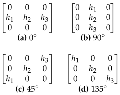
For the convolution process, we define four $3\times 3$ convolution masks or kernels with respect to four directions $0^{\circ }$, ${45}^{\circ }$, ${90}^{\circ }$ and ${135}^{\circ }$. These directional kernels are shown in Figure 1.

The Hankel determinants $h_1,h_2$ and $h_3$ are derived using the Equations (4), (5) and (8). ⋋ = 0.5 is substituted in these equations and achieve the values $h_1=0.5$, $h_2=0.14063$ and $h_3=0.104167$. These determinant values are used as weights in image enhancement. This choice of ⋋ value enhances image quality, structural integrity and overall robustness in method.

The proposed algorithm is as follows (Algorithm 1):

Algorithm 1 Proposed Image Enhancement Algorithm based on Hankel Determinants

Step 1: Read input image I (grayscale or RGB) and convert to double precision. Step 2: Extract dimensions $M\times N\times C$. For medical imagery, the channel C is typically 1 (grayscale), whereas, for color datasets, the algorithm processes each channel independently. Set the class parameter $⋋=0.5$. Step 3: Define four $3\times 3$ kernels ${\mathrm{KerH}}_1,{\mathrm{KerH}}_2,{\mathrm{KerH}}_3,{\mathrm{KerH}}_4$ for four directions $0^{\circ }$, ${45}^{\circ }$, ${90}^{\circ }$ and ${135}^{\circ }$. The kernels are illustrated in Figure 1. Zero-padding is employed during convolution to preserve image dimensions. Step 4: For each channel $c=1$ to C, compute convolution using, $K_i=I_c\ast {\mathrm{KerH}}_i,fori=1,2,3,4.$ For grayscale images, convolution is directly applied to the single-channel image. For RGB images, each channel is processed independently using the four directional kernels. Step 5: Isolate the high-frequency structural details by computing the difference between the original signal and the filtered output using $D_i=I_c-K_i.$ Step 6: Perform pixel-wise maximum selection for capturing the most prominent directional features at each pixel using $D_{\max }=max(D_1,D_2,D_3,D_4).$ Step 7: Generate the final enhanced image by using, $I_{\mathrm{enh},c}=I_c+⋋·D_{\max }$. Step 8: Clip all enhanced intensity values outside the interval $[0,255]$, and convert the reconstructed image back to $uint8$ representation. Step 9: If the image is RGB, convert original and enhanced images to grayscale for analysis. Step 10: Compute the probability density function (PDF) and cumulative distribution function (CDF) and compare PDF/CDF between original and enhanced images. Generate mesh representations of original and enhanced images for 3D visualization of pixel intensities. Step 11: Evaluate performance metrics including Mean Squared Error (MSE), Peak Signal-to-Noise Ratio (PSNR), Standard Deviation (SD), Pearson Correlation Coefficient (PCC), and Structural Similarity Index (SSIM). Step 12: Display the enhanced image. The total computational complexity is $O(M\times N\times C)$, as the four convolutions are performed in parallel per channel.

All convolution operations were implemented using zero-padding at image boundaries in order to preserve the original spatial dimensions throughout the enhancement process. The proposed directional kernels were normalized prior to filtering to avoid excessive amplification of intensity values. During implementation, input images were first converted from uint8 format to double precision within the interval [0, 255]. After enhancement, all reconstructed pixel values exceeding the valid intensity range were clipped to the interval [0, 255] before reconversion to uint8 format.

For RGB images, the enhancement procedure was applied independently to each color channel, whereas grayscale medical images were processed directly as single-channel inputs. The directional convolution masks corresponding to 0°, 45°, 90°, and 135° orientations were applied separately, and the maximum directional response was selected pixel-wise to preserve dominant structural information.

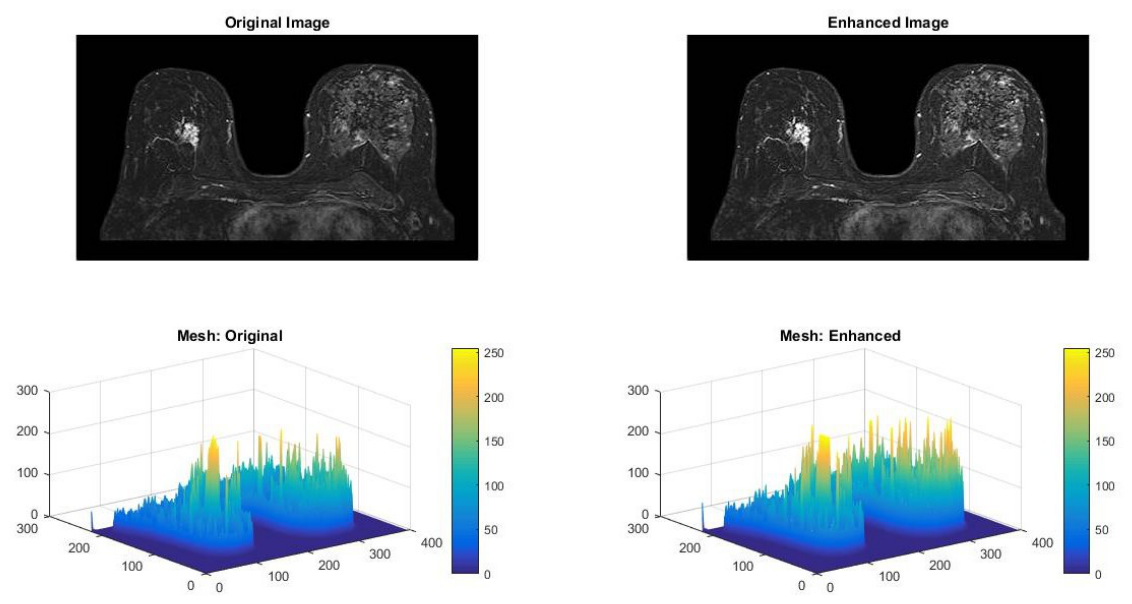
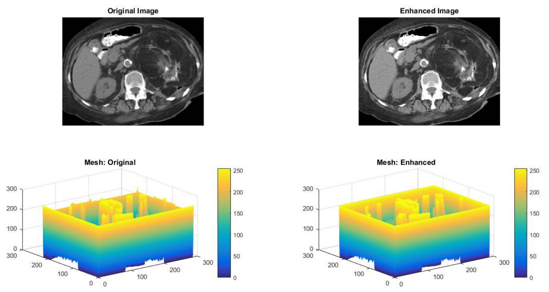
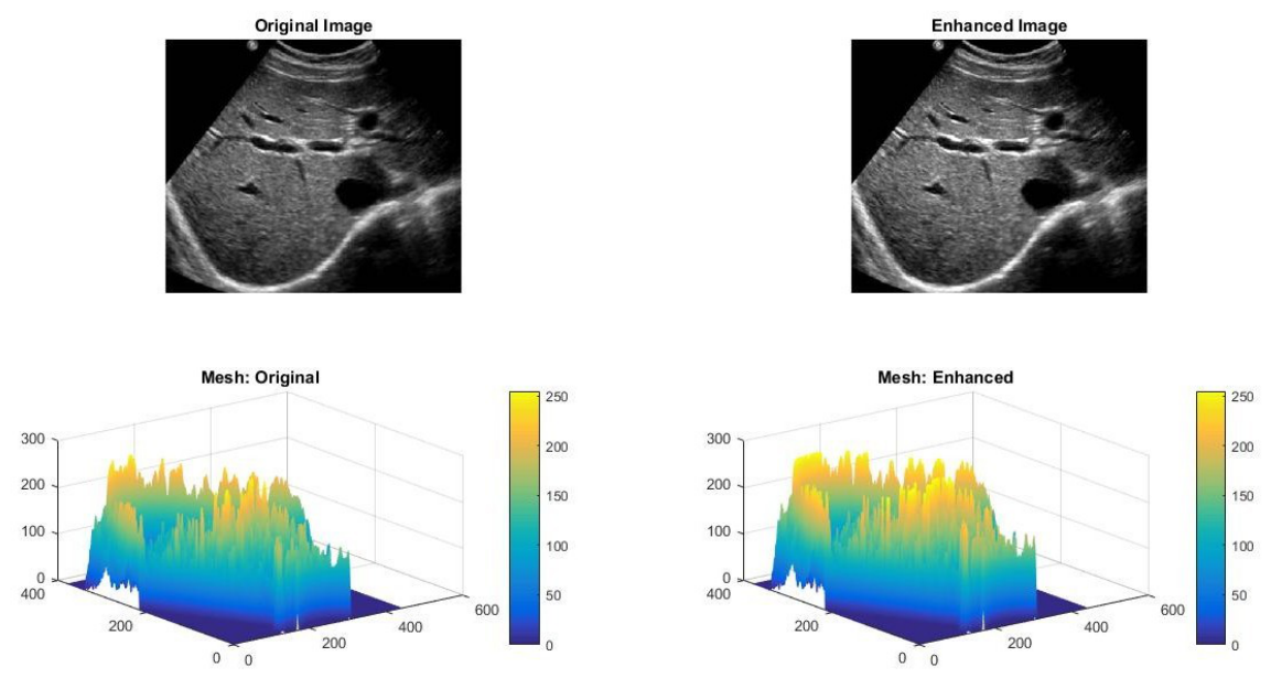
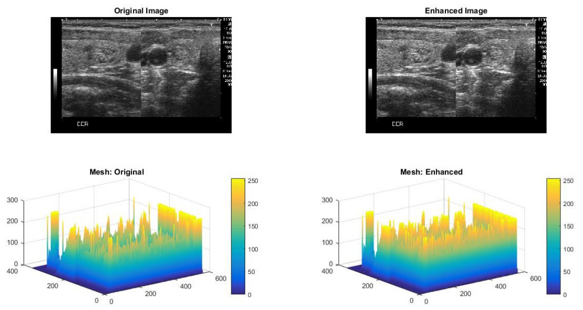
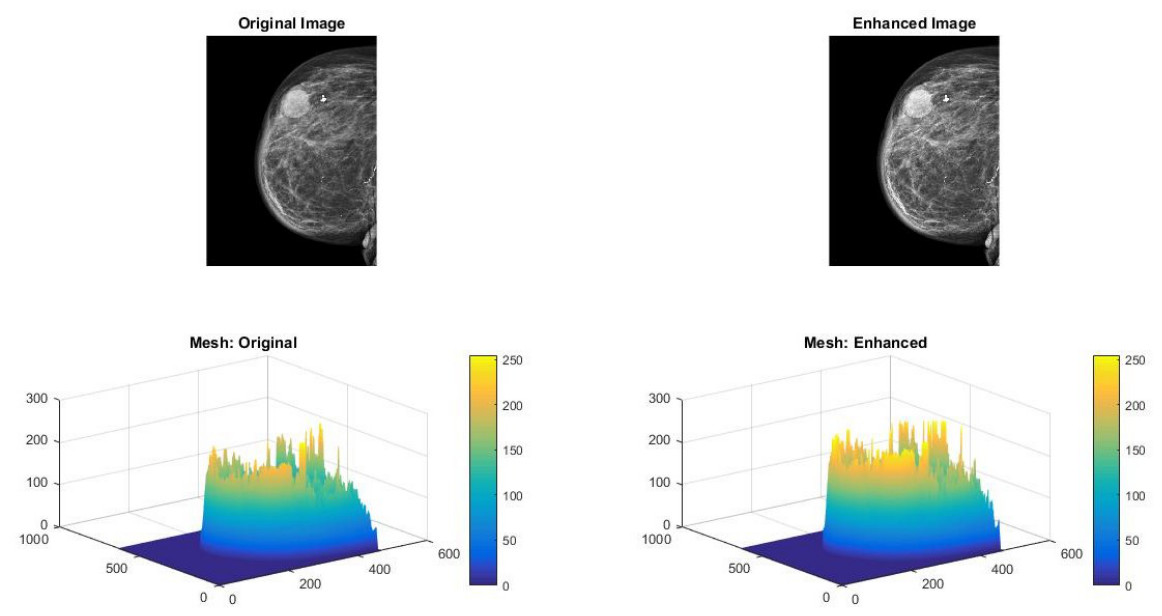
We tested our proposed algorithm on four medical images, including Brain Cancer, retinal infection, Liver and Thyroid Ultrasound as given in Figure 2, Figure 3, Figure 4 and Figure 5. The original images exhibit a hazy effect that obscures structural details like small nodules in thyroid scans and micro calcification in breast tissues. By implementing the enhancement kernels, the enhanced images exhibit a significant restoration of structural clarity, like boundary sharpening in Breast cancer and Renal infection images, and in the Liver and Thyroid ultrasounds, the granular speckle noise of the ultrasound is effectively regularized. Our method presents visually improved enhancement.

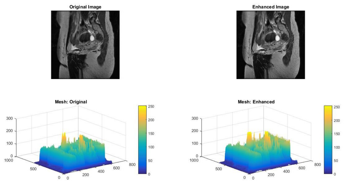
In order to further investigate the mathematical influence of the proposed method on the image enhancement, 3D mesh representations are utilized as shown in Figure 2, Figure 3, Figure 4 and Figure 5. These mesh plots capture the geometric stability of the images by interpreting the pixel intensity as the height, that is, the z-axis of a topological surface. The mesh representations of the original images represent relatively flat and chaotic topography, whereas the enhanced mesh plots show distinct intensity peaks and localized gradients. This topographic sharpening provides a clearer map for Computer Aided Diagnosis (CAD).

The quantitative evaluation of the proposed method is analyzed using the quality metrics such as Mean Squared Error (MSE) [44], Peak Signal-to-Noise Ratio (PSNR) [44], Standard Deviation (SD) [26], Pearson Correlation Coefficient (PCC) [27], and Structural Similarity Index (SSIM) [45].

Table 1. Quantitative evaluation of the proposed enhancement method on four medical ultrasound images using Mean Squared Error (MSE), Peak Signal-to-Noise Ratio (PSNR), Standard Deviation (SD), Pearson Correlation Coefficient (PCC), and Structural Similarity Index (SSIM) metrics.

Image	MSE	PSNR	SD	PCC	SSIM
Breast Cancer	55.634729	30.677344	34.157156	0.997680	0.974957
Renal Infection	172.124246	25.772383	63.231818	0.995429	0.965032
Liver Ultrasound	123.996716	27.196702	56.726536	0.999269	0.977606
Thyroid Ultrasound	166.009732	25.929468	57.980851	0.997101	0.965452

shows the values for the performance evaluation of the proposed method. The algorithm consistently achieved better quality metrics for each image, thus outperforming the compared histogram-based methods (QDHE and CLAHE).

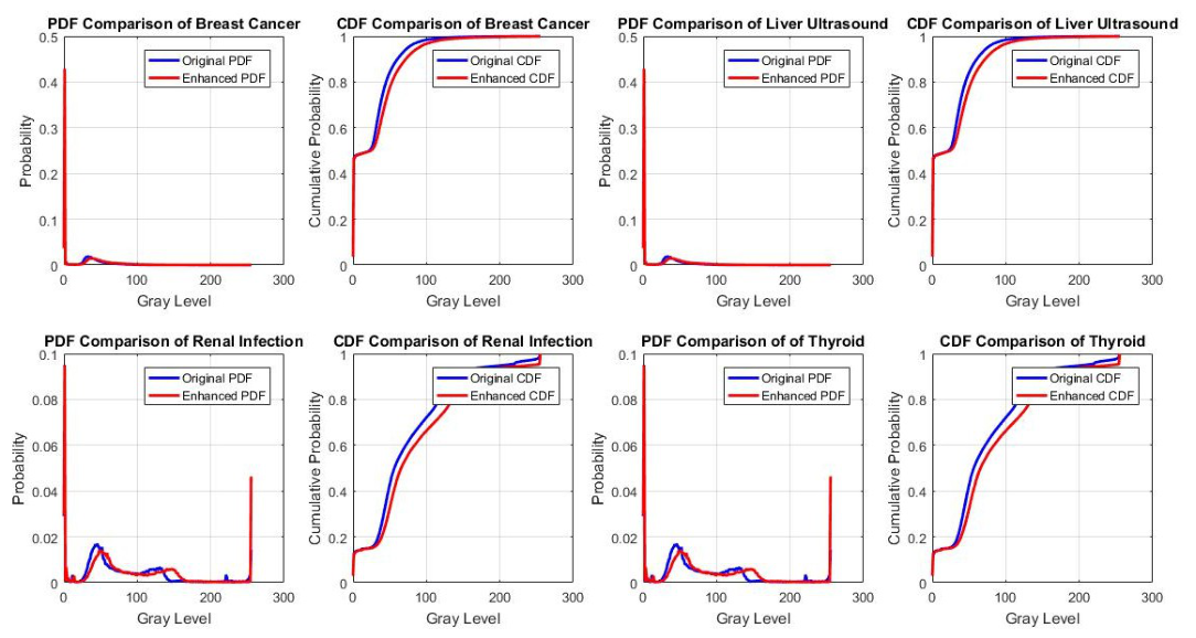
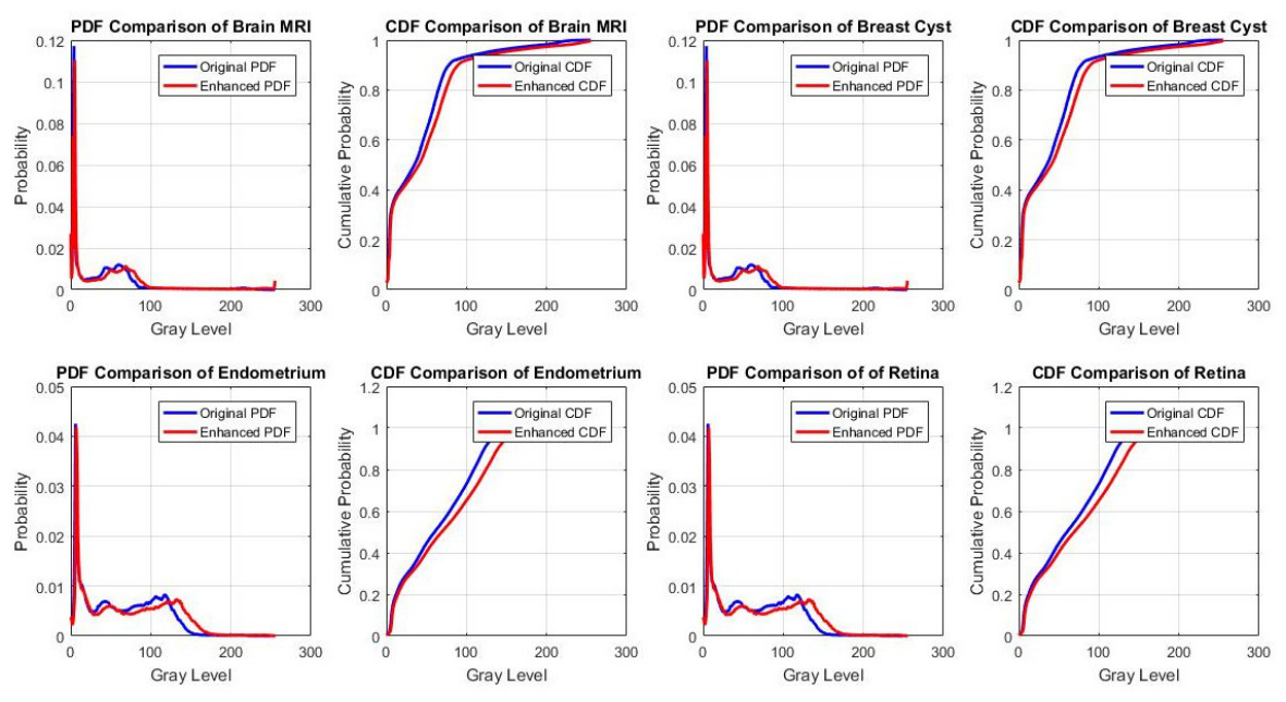
The PDF and CDF comparison as shown in Figure 6, demonstrates the effectiveness of the proposed method for Brain Cancer, renal infection, Liver and Thyroid Ultrasound images. The original PDF for these medical images is narrow and peaked, which indicates the low contrast. In contrast, the PDF of enhanced images spread over a wide range of gray levels and exhibits a flatter shape. This corresponds to a significant increase in image contrast. Moreover, the peak of enhanced PDF is lower than the original, which confirms the preservation of natural tissue appearance. The CDF comparison further supports these observations. The CDF for original images rises slowly and saturates early, showing that most pixels are concentrated in a narrow intensity band. In contrast, the CDF of the enhanced image becomes steeper, indicating that the enhancement algorithm has successfully stretched the intensity histogram, which preserves the fine structures in the image. Together, the PDF and CDF analyses provide statistical evidence that the proposed enhancement method significantly improves the image quality as compared to the original.

6. Comparative Analysis

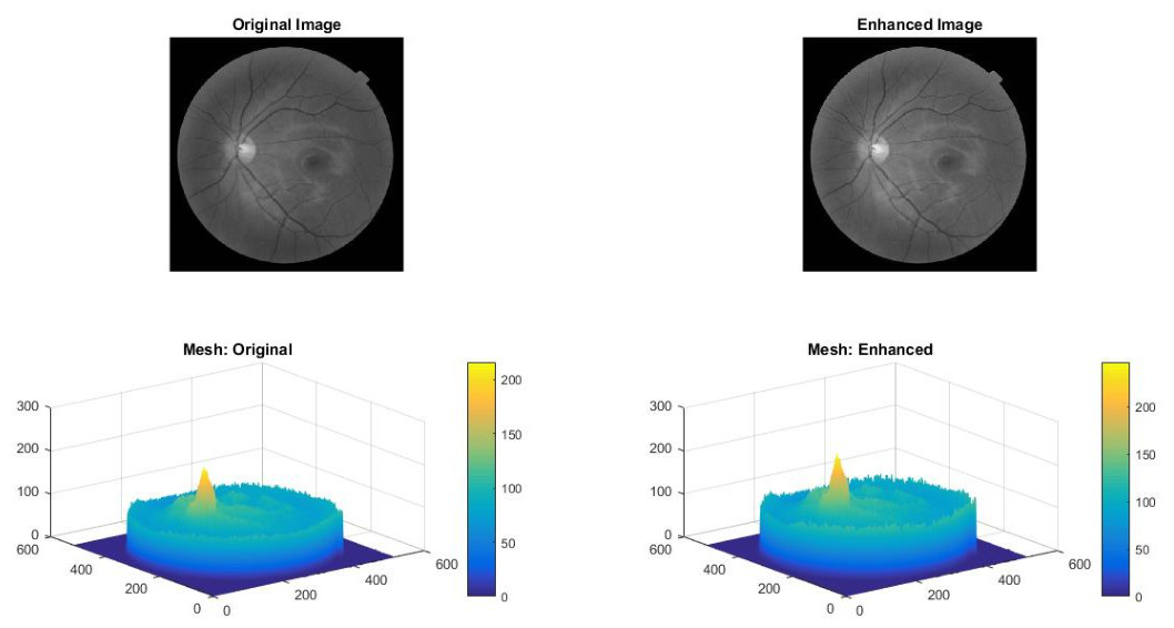
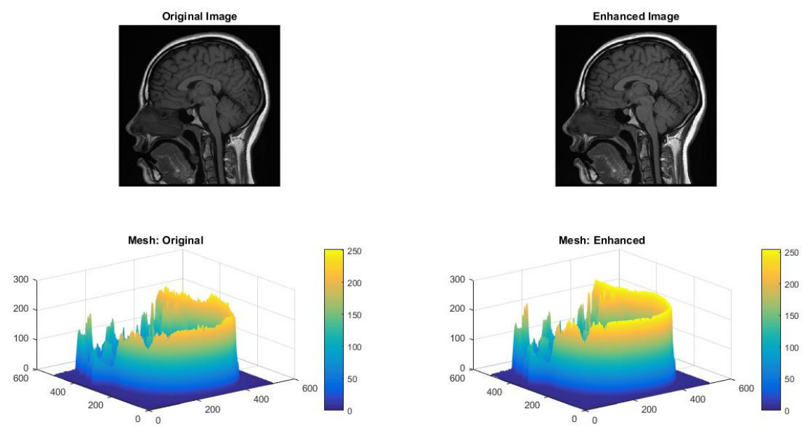
In order to further validate the effectiveness of our proposed enhancement algorithm, we compare it with the histogram-based method provided by Salem et al. [29] in 2019. In their study four histogram based techniques, including HE, CHE, QDHE and CLAE, are evaluated on medical images. Among these methods, QDHE and CLAE outperformed the other two methods. Therefore, we select QDHE and CLAE methods for comparison with our proposed method. We perform our proposed algorithm on four medical images, including Retina, Brain MRI, Breast cyst, and Endometrium MRI. Figure 7, Figure 8, Figure 9 and Figure 10 demonstrate that our proposed method provides visually enhanced images with sharper edges, better contrast and more natural intensity distribution than both histogram-based methods.

Figure 11 demonstrates the CDF and PDF comparison of original and enhanced retina, MRI-brain, MRI-endometrium, and breast cyst images. Thus, validating the proposed image enhanced procedure.

For quantitative assessment, we compute the same three metrics used in [29], including, Mean Square Error (MSE), Peak Signal-to-Noise Ratio (PSNR), and Standard Deviation (SD).

The methods QDHE and CLACHE used in

Table 2. Comparison of Mean Square Error (MSE).

Image	QDHE [29]	CLAHE [29]	Proposed
Retina	1174.3	223.0449	87.597301
Brain MRI	670.8361	1261.2	79.793144
Endometrium	902.5713	1152.0	121.345760
Breast cyst	765.4772	770.9151	108.841546
Average	878.29615	851.79	99.39437

,

Table 3. Comparison of Peak Signal-to-Noise Ratio (PSNR in dB).

Image	QDHE [29]	CLAHE [29]	Proposed
Retina	17.43330	21.2357	28.705896
Brain MRI	19.8646	14.5745	29.111148
Endometrium	18.5760	14.9021	27.290558
Breast cyst	19.2915	18.0190	27.762857
Average	18.791350	17.182825	28.217615

and

Table 4. Comparison of Standard Deviation (SD).

Image	QDHE [29]	CLAHE [29]	Proposed
Retina	60.1603	47.4125	45.637713
Brain MRI	60.8605	63.9431	49.075249
Endometrium	66.3201	66.6786	51.382256
Breast cyst	71.2628	70.8172	59.139729
Average	64.650925	62.212850	51.308737

, the computation time for these methods is 0.180992 CPU seconds.

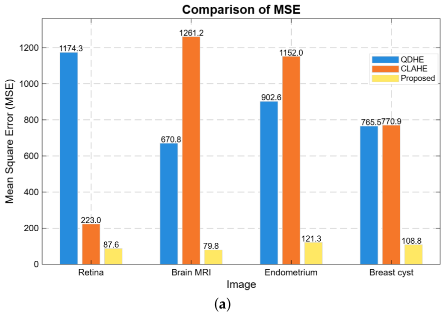
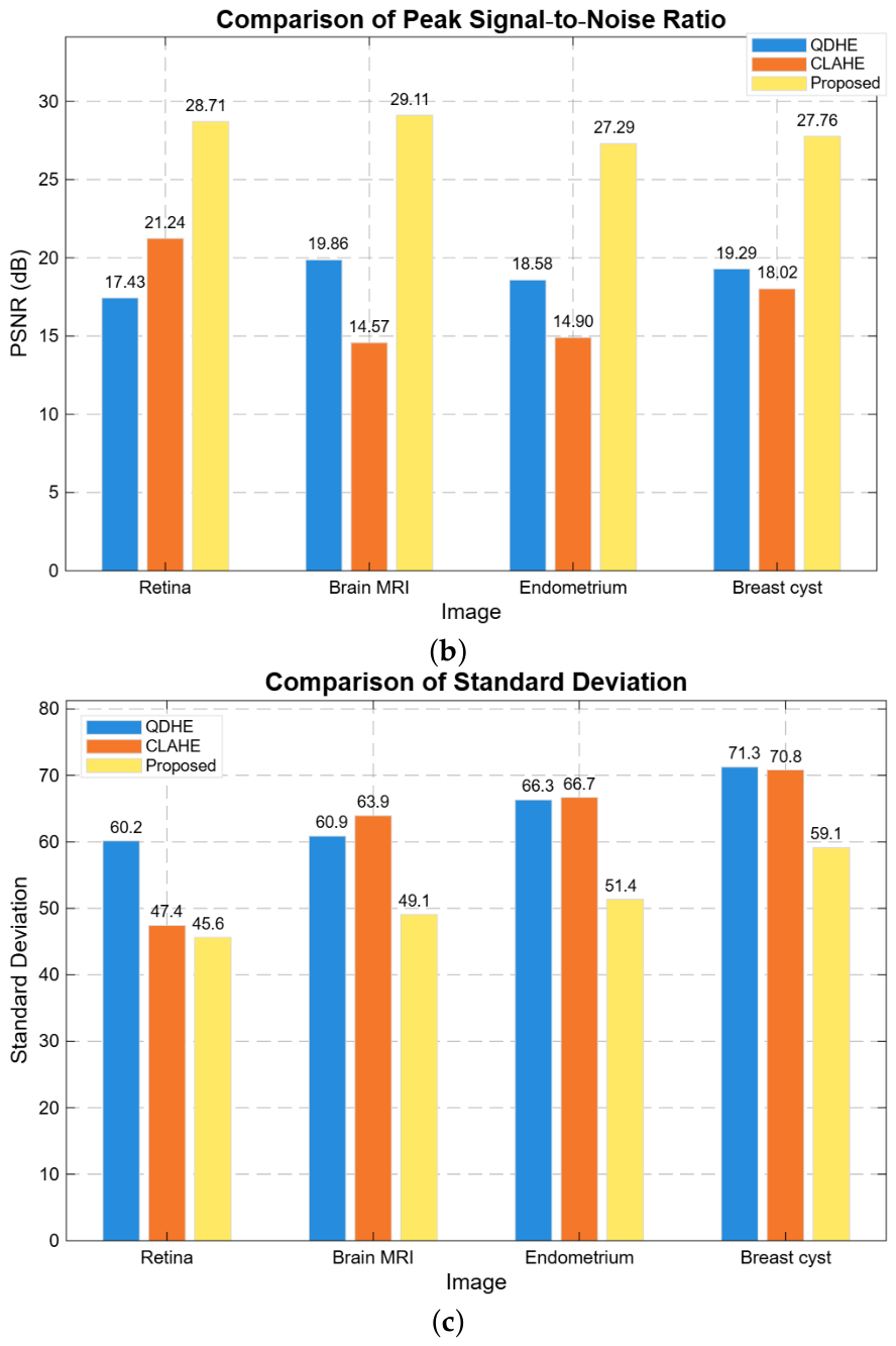
From the Table 2, Table 3 and Table 4, and Figure 12, it is clear that the proposed algorithm outperforms both QDHE and CLAHE across all the four images. In terms of MSE, the proposed method achieves an average value of 99.39, which is the lower compared to QDHE and CLAHE. Similarly, the average PSNR value for the proposed method is 28.2176 dB which higher compared to both QDHE and CLAE. Additionally, the average SD value for the proposed method is 51.30873 indicating the superiority of our proposed algorithm over conventional histogram-based techniques. These results show that our Hankel determinant-based algorithm consistently outperforms the leading histogram-based techniques, including QDHE and CLAE, in terms of noise reduction, structural preservation, and contrast enhancement. This advancement is particularly important for low-contrast images, where traditional histogram equalization methods frequently struggle to preserve fine details.

7. Ablation Study and Sensitivity Analysis

To rigorously evaluate the contribution of each component in the proposed framework, we conduct an ablation study summarized in

Table 5. Ablation study comparing full method against variants without Hankel weights and without directional diversity. Results are reported as PSNR (dB)/SSIM for each image. The full method uses $⋋=0.5$, all four directional kernels, Hankel weights $h_1,h_2,h_3$, and max selection.

Image	Full Method	No Hankel Weights	Single Direction (90°)
Brain Cancer	30.68/0.975	26.12/0.913	27.91/0.942
Renal Infection	25.77/0.965	21.34/0.901	22.98/0.931
Liver Ultrasound	27.20/0.978	22.71/0.916	24.45/0.946
Thyroid Ultrasound	25.93/0.965	21.52/0.904	23.08/0.934
Average	27.40/0.971	22.92/0.909	24.61/0.938

.

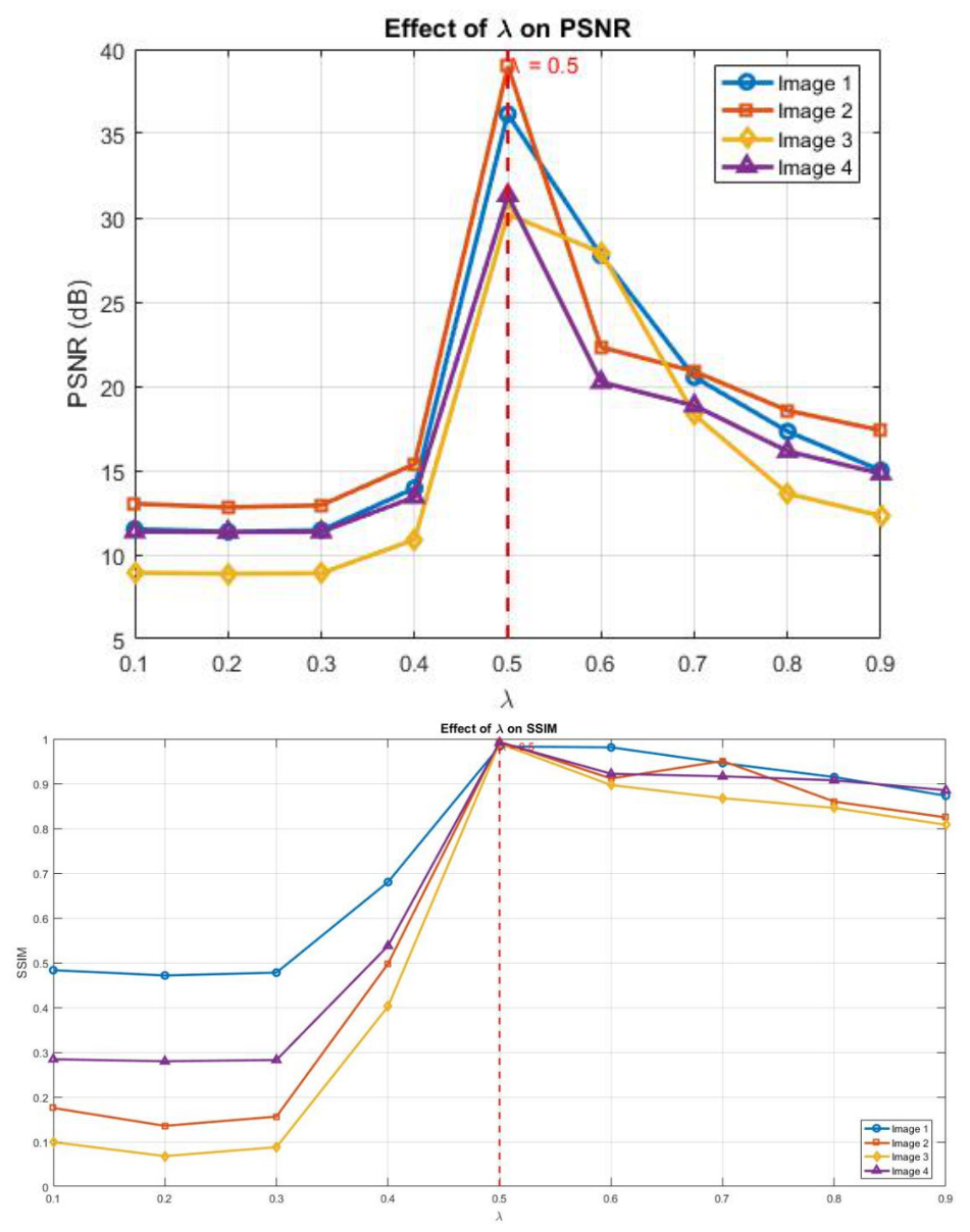
The table reports PSNR and SSIM values for the Full Method (Hankel weights, four directional kernels with max selection, and $⋋=0.5$ against two variants: No Hankel Weights (Uniform), where the Hankel determinants are replaced by uniform weights, and Single Direction Only $\left({90}^{\circ }\right)$, where only one directional kernel is used without max selection. The Full Method consistently achieves the highest PSNR and SSIM across all four medical images, confirming that both the Hankel-based adaptive weights and the multi-directional fusion strategy are essential for optimal enhancement. Furthermore, to determine the optimal value of the parameter ⋋ we perform a sensitivity analysis by varying ⋋ from 0.1 to 0.9. The results are illustrated in Figure 13.

Figure 13 illustrates that both PSNR and SSIM achieve good performance as ⋋ increase from 0 to 0.5. After this point, the performance of both metrics gradually decrease. The control parameter ⋋ determines the enhancement strength during reconstruction. Based on experimental analysis using PSNR and SSIM curves, ⋋ = 0.5 provided the best balance between contrast enhancement and structural preservation, and was therefore adopted throughout all experiments. Therefore, ⋋ = 0.5 is selected as optimal parameter.

Although recent deep learning and Retinex-based enhancement methods have demonstrated strong performance in medical imaging applications, many such approaches rely on large-scale supervised training, iterative optimization, or computationally expensive architectures. The proposed Hankel determinant-based framework offers a lightweight alternative with low computational complexity and no training requirement. This makes the method particularly attractive for rapid preprocessing, portable diagnostic systems, and scenarios with limited computational resources.

Moreover, unlike purely data-driven models, the proposed approach is derived from analytically established coefficient bounds associated with bi-univalent functions, thereby providing a mathematically interpretable enhancement mechanism. Future work will focus on extending the comparative experiments to include lightweight CNN-based and Retinex-based enhancement models on larger benchmark datasets.

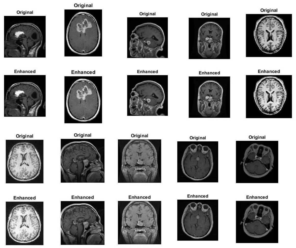
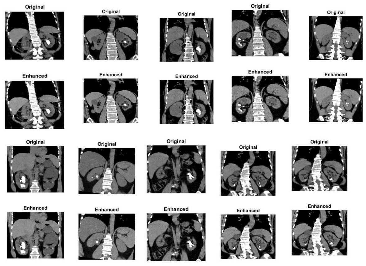
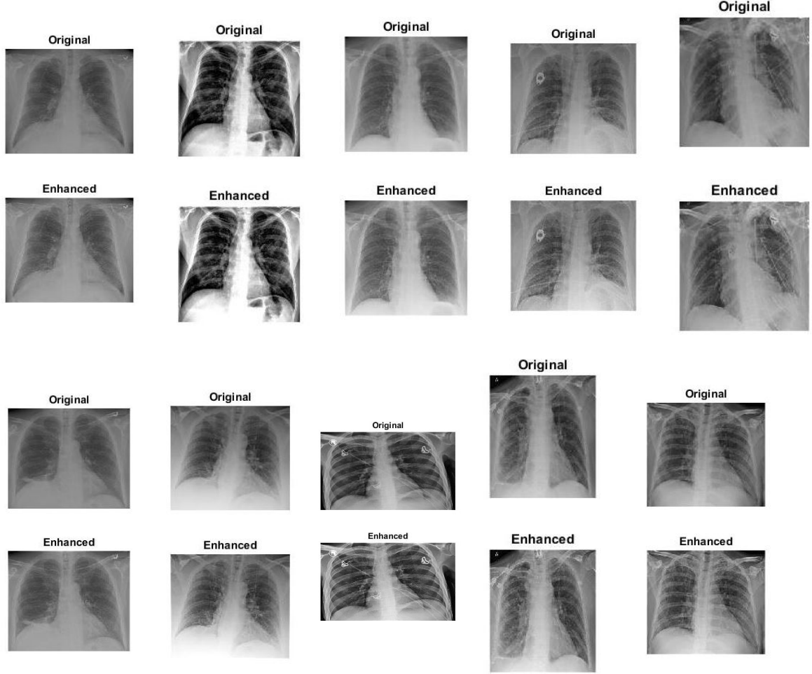
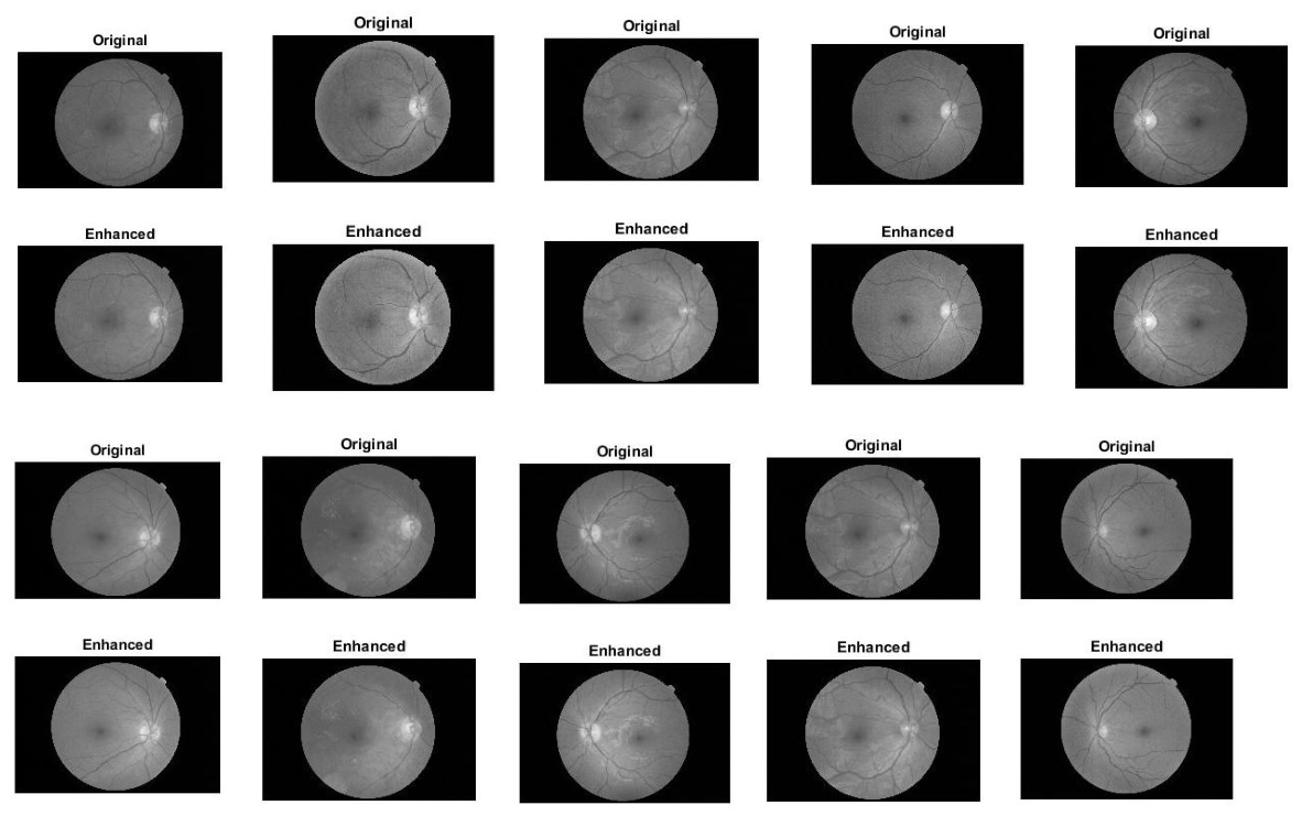
We have also tested our proposed algorithm on different medical datasets. Each dataset contains 10 images to ensure consistent evaluation and the improvement is largest dataset proves the robustness of our proposed method.

Table 6. Performance metrics for original and enhanced medical images.

Image	MSE	PSNR	PCC	SSIM
Brain MRI	152.054143	27.279793	0.998720	0.977446
Kidney stone	159.439565	26.125318	0.996797	0.969800
Corona Virus	334.244384	22.924309	0.996730	0.949688
Messidor Dataset	97.015478	28.286499	0.999757	0.986438

shows that quantitative metrics show remarkable improvement across all datasets. A clear enhancement of images can also be viewed in Figure 14, Figure 15, Figure 16 and Figure 17. An average PSNR, SSIM, PCC and MAE metric values are calculated for these datasets to provide more reliable and robust evaluation of proposed method.

8. Limitations

It should be noted that the medical image datasets employed in this study do not provide corresponding ideal ground-truth enhanced images. Therefore, the original medical images are treated as baseline reference images for quantitative assessment. In this context, PSNR, MSE, and SSIM are utilized as relative quality indicators to evaluate the extent to which the enhancement process preserves structural information while improving visual contrast and edge visibility.

Specifically, PSNR and MSE are interpreted as measures of distortion introduced during enhancement, whereas SSIM and PCC quantify the preservation of anatomical structures and local intensity relationships. Since medical image enhancement aims to improve diagnostic visibility without significantly altering the intrinsic structural content of the image, these metrics remain appropriate for comparative analysis with existing enhancement techniques.

We acknowledge that full-reference metrics may not completely characterize perceptual enhancement quality in the absence of pristine ground-truth images. Therefore, the quantitative evaluation is further supported through PDF/CDF analysis, mesh visualization, and comparative visual assessment against established enhancement methods.

Moreover, it is worth mentioning that the present comparison is intentionally limited to histogram-based enhancement methods (QDHE and CLAHE), as these share the training-free, low-complexity characteristics of our proposed framework; comparisons with Retinex, denoising-only, or deep learning baselines involve fundamentally different assumptions and are therefore reserved for future work.

9. Conclusions

This work presents a novel framework that connects geometric function theory with practical image enhancement. A new subclass of bi-univalent functions $\mathcal{B}(\hslash )$ was introduced, and sharp bounds for its associated Hankel determinants were established. These analytically derived quantities were then utilized to construct directional convolution kernels, leading to a mathematically grounded and computationally efficient enhancement algorithm.

The proposed method was evaluated on a range of medical images, where it consistently improved contrast, preserved structural details, and enhanced edge clarity. Quantitative assessments based on PSNR, SSIM, MSE, SD, and PCC further support the effectiveness of the approach in comparison with conventional enhancement techniques. The ablation study confirmed that Hankel weights contribute approximately 4.5 dB and directional fusion contributes approximately 2.8 dB to the average PSNR compared to uniform weighting or single-direction convolution. Sensitivity analysis demonstrated that ⋋ = 0.5 is globally optimal across all test images, with stable performance across $⋋\in [0,1]$. Mesh plot analyses visually confirmed that enhanced images exhibit sharper intensity gradients and better-preserved anatomical boundaries.Unlike data-driven models, the method does not require training data and maintains low computational complexity, making it suitable for practical deployment.

Beyond its immediate application, this study highlights the potential of using coefficient-based structures from analytic function theory in image processing tasks. At the same time, the present comparison is limited to histogram-based baselines (QDHE and CLAHE), as these share the training-free, low-complexity characteristics of our method; comparisons with Retinex, denoising-only, or deep learning approaches involve fundamentally different assumptions and are reserved for future work. The parameter ⋋ remains fixed rather than adaptive, and the current implementation is restricted to still images, not yet extended to video or 3D medical volumes. Additionally, the theoretical bounds assume analytic idealizations that may not fully capture all real-world image degradations.

Despite these limitations, the proposed framework demonstrates a meaningful and productive bridge between analytic function theory and practical medical image enhancement, offering a mathematically grounded, training-free alternative to conventional and deep learning-based approaches.

References

1. Robertson, M.S. Certain classes of starlike functions. Mich. Math. J. 1985, 32, 135–140. [Google Scholar] [CrossRef]
2. Brannan, D.A.; Taha, T.S. On some classes of bi-univalent functions. Stud. Univ. Bolyai Math. 1986, 31, 70–77. [Google Scholar]
3. Taha, T.S. Topics in Univalent Function Theory. Ph.D. Thesis, University of London, London, UK, 1981. [Google Scholar]
4. Netanyahu, E. The minimal distance of the image boundary from the origin and the second coefficient of a univalent function in |z|. Arch. Ration. Mech. Anal. 1969, 32, 100–112. [Google Scholar] [CrossRef]
5. Srivastava, H.M.; Mishra, A.K.; Gochhayat, P. Certain subclasses of analytic and bi-univalent functions. Appl. Math. Lett. 2010, 23, 1188–1192. [Google Scholar] [CrossRef]
6. Tang, H.; Deng, G.-T.; Li, S.-H. Coefficient estimates for new subclasses of Ma-Minda bi-univalent functions. J. Ineq. Appl. 2013, 2013, 317. [Google Scholar] [CrossRef]
7. Deniz, E. Certain subclasses of bi-univalent functions satisfying subordinate conditions. J. Class. Anal. 2013, 2, 49–60. [Google Scholar] [CrossRef]
8. Srivastava, H.M.; Murugusundaramoorthy, G.; Bulboaca, T. The second Hankel determinant for subclasses of Bi-univalent functions associated with a nephroid domain. Rev. R. Acad. Cienc. Exactas Fís. Nat. Ser. A Mat. 2022, 116, 145. [Google Scholar] [CrossRef]
9. Vijaya, K.; Murugusundaramoorthy, G. Bi-starlike function of complex order involving Mathieu-type series associated with telephone Numbers. Symmetry 2023, 15, 638. [Google Scholar] [CrossRef]
10. Hosseini, S.H.; Motamednezhad, A.; Salehian, S. Coefficient estimates for a subclass of analytic and bi-univalent functions by an integral operator. Int. J. Nonlinear Anal. Appl. 2025, 16, 179–187. [Google Scholar]
11. Noonan, W.; Thomas, D.K. On the second Hankel determinant of a really mean p-valent functions. Trans. Am. Math. Soc. 1976, 223, 337–346. [Google Scholar]
12. Zeyani, A.; Hussen, A. Second Hankel Determinant for a Bi-univalent Function Subclass Based Gegenbauer (Ultraspherical) Polynomials. Eur. J. Pure Appl. Math. 2025, 18, 5968. [Google Scholar] [CrossRef]
13. Ali, E.E.; Srivastava, H.M.; Kota, W.Y.; El-Ashwah, R.M.; Albalah, A.M. The second Hankel determinant and the Fekete-Szegö functional for a subclass of analytic functions by using the q-Sălăgean derivative operator. Alex. Eng. J. 2025, 116, 141–146. [Google Scholar] [CrossRef]
14. Fekete, M.; Szegö, G. Eine Bemerkung über ungerade Schlichte Funktionen. J. Lond. Math. Soc. 1933, 1, 85–89. [Google Scholar] [CrossRef]
15. Babalola, K.O. On H3(1) Hankel determinant for some classes of univalent functions. In Inequality Theory and Applications; Nova Science Publishers, Inc.: Hauppauge, NY, USA, 2010; Volume 6, pp. 1–7. [Google Scholar]
16. Orhan, H.; Çaglar, M.; Cotirla, L.-I. Third Hankel Determinant for a Subfamily of Holomorphic Functions Related with Lemniscate of Bernoulli. Mathematics 2023, 11, 1147. [Google Scholar] [CrossRef]
17. Buyankara, M.; Çaglar, M. Hankel and Toeplitz determinants for a subclass of analytic functions. Mat. Stud. 2023, 60, 132–137. [Google Scholar] [CrossRef]
18. Hu, W.; Deng, J. Hankel Determinants, Fekete-Szegö Inequality, and Estimates of Initial Coefficients for Certain Subclasses of Analytic Functions. AIMS Math. 2024, 9, 6445–6467. [Google Scholar] [CrossRef]
19. Gebur, S.K.; Atshan, W.G. Second Hankel Determinant and Fekete–Szegö Problem for a New Class of Bi-Univalent Functions Involving Euler Polynomials. Symmetry 2024, 16, 530. [Google Scholar] [CrossRef]
20. Srivastava, H.M.; Shaba, T.G.; Ibrahim, M.; Tchier, F.; Khan, B. Coefficient Bounds and Second Hankel Determinant for a Subclass of Symmetric Bi-Starlike Functions Involving Euler Polynomials. Bull. Sci. Math. 2024, 192, 103405. [Google Scholar] [CrossRef]
21. Hadi, S.H.; Darus, M.; Ibrahim, R.W. Third-order Hankel determinants for q-analogue analytic functions defined by a modified q-Bernardi integral operator. Quaest. Math. 2024, 47, 2109–2131. [Google Scholar] [CrossRef]
22. Hussen, A.; Illafe, M.; Zeyani, A. Fekete-Szegö and Second Hankel Determinant for a Certain Subclass of Bi-Univalent Functions associated with Lucas-Balancing Polynomials. Int. J. Neutrosophic Sci. 2025, 25, 417–434. [Google Scholar]
23. Amini, E.; Al-Omari, S. Subordination Properties of Bi-Univalent Functions Involving Horadam Polynomials. J. Funct. Spaces 2025, 2025, 4388121. [Google Scholar] [CrossRef]
24. Tayyah, A.S.; Atshan, W.G. Starlikeness and bi-starlikeness associated with a new Carathéodory function. J. Math. Sci. 2025, 290, 232–256. [Google Scholar] [CrossRef]
25. Al-Ityan, M.; Amourah, A.; Alsoboh, A.; Anakira, N.; Raba’a, M.B.; Hammad, S.; Sasa, T. Fekete–Szegő inequalities for a new class of bi-univalent functions defined via the Mittag-Leffler function. Eur. J. Pure Appl. Math. 2025, 18, 6064. [Google Scholar] [CrossRef]
26. Gonzalez, R.C.; Woods, R.E. Digital Image Processing, 4th ed.; Pearson: London, UK, 2018. [Google Scholar]
27. Wang, Z.; Bovik, A.C. Modern Image Quality Assessment; Morgan & Claypool Publishers: San Rafael, CA, USA, 2006. [Google Scholar]
28. Lecca, M.; Simone, G.; Bonanomi, C.; Rizzi, A. Point-based spatial colour sampling in Milano-Retinex: A survey. IET Image Process. 2018, 12, 833–849. [Google Scholar] [CrossRef]
29. Salem, N.; Malik, H.; Shams, A. Medical image enhancement based on histogram algorithms. In Proceedings of the 16th International Learning & Technology Conference 2019; Elsevier: Amsterdam, The Netherlands, 2019. [Google Scholar]
30. Duren, P.L. Univalent Functions. In Grundlehren der Mathematischen Wissenschaften, Band 259; Springer: New York, NY, USA; Berlin/Hidelberg, Germany; Tokyo, Japan, 1983. [Google Scholar]
31. Nandhini, B.; Sruthakeerthi, B. Investigating the quality measures of image enhancement by convoluting the coefficients of analytic functions. Eur. Phys. J. Spec. Top. 2024, 234, 2647–2657. [Google Scholar] [CrossRef]
32. Al-Ameedee, S.A.; Atshan, W.G.; Al-Maamori, F.A. Second Hankel determinant for certain subclasses of bi-univalent functions. J. Phys. Conf. Ser. 2020, 1664, 012044. [Google Scholar] [CrossRef]
33. Liu, D.; Ahmad, A.; Ikhlas, H.; Hussain, S.; Noor, S.; Tang, H. On Sharp Coefficients and Hankel Determinants for a Novel Class of Analytic Functions. Axioms 2025, 14, 191. [Google Scholar] [CrossRef]
34. Aarthy, B.; Keerthi, B.S. Enhancement of various images using coefficients obtained from a class of Sakaguchi type functions. Sci. Rep. 2023, 13, 18722. [Google Scholar] [CrossRef]
35. Priya, H.; Sruthakeerthi, B. Texture analysis using Horadam polynomial coefficient estimate for the class of Sakaguchi kind function. Sci. Rep. 2023, 13, 14436. [Google Scholar] [CrossRef]
36. Nithiyanandham, E.K.; Keerthi, B.S. A new proposed model for image enhancement using the coefficients obtained by a subclass of the Sakaguchi-type function. Signal Image Video Process. 2024, 18, 1455–1462. [Google Scholar] [CrossRef]
37. Nithiyanandham, E.K.; Keerthi, B.S. Image edge detection enhancement using coefficients of Sakaguchi type functions mapped onto petal shaped domain. Heliyon 2024, 10, e31430. [Google Scholar] [CrossRef]
38. Sundari, K.S.; Keerthi, B.S. Enhancing low-light images using Sakaguchi type function and Gegenbauer polynomial. Sci. Rep. 2024, 14, 29679. [Google Scholar] [CrossRef]
39. Khalil, A.M.; El-Bendary, M.A.; Hassanien, A.E. CDAN: Convolutional Dense Attention-Guided Network for Low-Light Image Enhancement. arXiv 2023, arXiv:2308.12902. [Google Scholar]
40. Grenander, U.; Szegö, G. Toeplitz Forms and Their Applications, California Monographs in Mathematical Sciences; University California Press: Berkeley, CA, USA, 1958. [Google Scholar]
41. He, K.; Sun, J.; Tang, X. Single image haze removal using dark channel prior. IEEE Trans. Pattern Anal. Mach. Intell. 2010, 33, 2341–2353. [Google Scholar] [CrossRef]
42. Dong, X.; Pang, Y.; Wen, J. Fast efficient algorithm for enhancement of low lighting video. In Proceedings of the ACM SIGGRAPH 2010 Posters, Los Angeles, CA, USA, 25–29 July 2010; p. 1. [Google Scholar]
43. Kanwal, B.; Iman, A.; Kanwal, S.; Alkhalifa, A.K. Estimation of Hankel inequalities of symmetric starlike functions in crescent-shaped domains and their application in image processing. Sci. Rep. 2025, 15, 27402. [Google Scholar] [CrossRef]
44. Girod, B. What’s wrong with mean-squared error. In Digital Images and Human Vision; MIT Press: Cambridge, MA, USA, 1993; pp. 207–220. [Google Scholar]
45. Jaya, V.L.; Gopikakumari, R. IEM: A new image enhancement metric for contrast and sharpness measurements. Int. J. Comput. Appl. 2013, 79, 1–9. [Google Scholar] [CrossRef]
Figure 1. Directional kernels.
Symmetry 18 01006 g001
Figure 2. Original vs. enhanced breast cancer ultrasound images with mesh plots.
Symmetry 18 01006 g002
Figure 3. Original vs. enhanced renal infection ultrasound images with mesh plots.
Symmetry 18 01006 g003
Figure 4. Original vs. enhanced liver ultrasound images with mesh plots.
Symmetry 18 01006 g004
Figure 5. Original vs. enhanced thyroid ultrasound images with mesh plots.
Symmetry 18 01006 g005
Figure 6. PDF and CDF comparison between original and enhanced Brain Cancer, renal infection, Liver and Thyroid Ultrasound images.
Symmetry 18 01006 g006
Figure 7. Original vs. enhanced Retina images with mesh plots.
Symmetry 18 01006 g007
Figure 8. Original vs. enhanced Brain MRI images with mesh plots.
Symmetry 18 01006 g008
Figure 9. Original vs. enhanced breast cyst images with mesh plots.
Symmetry 18 01006 g009
Figure 10. Original vs. enhanced Endometrium images with mesh plots.
Symmetry 18 01006 g010
Figure 11. PDF and CDF comparison between original and enhanced retina, MRI-brain, MRI-endometrium, and breast cyst images.
Symmetry 18 01006 g011
Figure 12. Comparison of image quality metrics: (a) Mean Squared Error (MSE) values; (b) Peak Signal-to-Noise Ratio (PSNR) values; (c) Standard Deviation (SD) values for QDHE, CLAHE, and the proposed method.
Symmetry 18 01006 g012aSymmetry 18 01006 g012b
Figure 13. Graph representing effect of ⋋ on PSNR and SSIM.
Symmetry 18 01006 g013
Figure 14. Different images of Brain MRI.
Symmetry 18 01006 g014
Figure 15. Different Images of Kidney stone.
Symmetry 18 01006 g015
Figure 16. Different Images of Corona Xrays.
Symmetry 18 01006 g016
Figure 17. Different Images of Messidor dataset.
Symmetry 18 01006 g017